Reconstruction of Short-Lived Particles using
Graph-Hypergraph Representation Learning

Abstract

In collider experiments, the kinematic reconstruction of heavy, short-lived particles is vital for precision tests of the Standard Model and in searches for physics beyond it. Performing kinematic reconstruction in collider events with many final-state jets, such as the all-hadronic decay of top-antitop quark pairs, is challenging. We present HyPER, a graph neural network that uses blended graph-hypergraph representation learning to reconstruct parent particles from sets of final-state objects. HyPER is tested on simulation and shown to perform favorably when compared to existing state-of-the-art reconstruction techniques, while demonstrating superior parameter efficiency. The novel hypergraph approach allows the method to be applied to particle reconstruction in a multitude of different physics processes.

I Introduction

The Large Hadron Collider (LHC) [1] at CERN produces 40 million high-energy proton-proton collisions per second to recreate the conditions of the early universe. These collisions frequently produce heavy, short-lived particles that promptly decay to relatively stable final states. Accurate reconstruction of these short-lived particles is critical for measuring their properties, and for defining observables which are sensitive to New Physics (NP). Further, the development of accurate and flexible methods for reconstructing short-lived particles in rare processes — like the production of top-antitop quark pairs with a Higgs boson, $t\bar{t}H$ — is a vital step in studying such rare topologies and scrutinizing the Standard Model (SM).

The kinematics of short-lived particles can only be inferred by considering the recorded kinematics of their decay products. The aim of the reconstruction process is to identify which combination of decay products corresponds to each parent particle. This task becomes increasingly challenging when we consider processes with many heavy resonances, such as the simultaneous production of four top quarks, $t\bar{t}t\bar{t}$: processes like these lead to high-multiplicity final states with large combinatorics.

The most common final-state objects produced at hadron colliders are jets: collimated sprays of neutral and charged hadrons which arise as a result of quantum chromodynamics (QCD). In addition to being produced in the decays of short-lived particles, jets can also arise from partonic splittings or concurrent proton-proton interactions. This increases the ‘jet-multiplicity’ of the final state and complicates the jet-assignment reconstruction problem. The case where heavy particles decay exclusively to jets is known as the all-hadronic decay channel. Particle reconstruction in this channel is simplified by the lack of final-state neutrinos, which go undetected and whose kinematics can only be partially inferred through conservation of momentum in the transverse plane.

A useful process for developing and benchmarking reconstruction techniques is the all-hadronic decay of $t\bar{t}$ pairs. Top quarks decay prior to hadronization through a near-exclusive decay channel $t\rightarrow Wb$. In the all-hadronic channel, both $W$ bosons then decay hadronically, with the full decay given by:

$$t\bar{t}\rightarrow W^{+}bW^{-}\bar{b}\rightarrow bq_{1}q_{2}\bar{b}q_{3}q_{4},$$ (1)

where the flavors of the $W$ boson decay products are distinct: $q_{1}\neq q_{2},q_{3}\neq q_{4}$. All six quarks in the final state will form jets, with jets originating from a $b$-quark referred to as ‘$b$-jets’. The example Feynman diagram in Fig. 1 shows the production and all-hadronic decay of a $t\bar{t}$ pair, with two additional jets produced through QCD radiation from an initial-state gluon. To reconstruct each top quark, we must identify which $b$-jet arises from each top quark decay, and identify the jet pair which arises from each subsequent $W$ boson decay. Techniques developed and validated in the all-hadronic $t\bar{t}$ channel can then be generalized to other collider processes with more complex final states.

Figure 1: A next-to-leading-order QCD Feynman diagram for the production of a $t\bar{t}$ pair through the fusion of two gluons, where both $W$ bosons decay hadronically. Two additional quarks ($q^{\prime}_{1}$ and $q^{\prime}_{2}$) are produced due to initial-state radiation (ISR). This leads to a final-state characterized by eight jets.

Reconstruction algorithms have seen a range of advancements in recent years. Two state-of-the-art machine learning (ML) approaches, developed initially for use in the all-hadronic $t\bar{t}$ channel, are SPANet [2, 3] and Topograph [4]. The former employs an attention mechanism which exploits the symmetry properties of $W$ boson decays to assign the correct final-state jets to their parent top quarks. The latter draws inspiration from Feynman diagrams and studies the relations between intermediate particles and their decay products. The use of advanced multivariate techniques in both cases allows the models to explore the complex relations between final states and the kinematics of the parent top quarks, leading to enhanced performance over existing $\chi^{2}$–minimization-based techniques [5, 2, 3, 4]. Both techniques are, however, characterized by networks with millions of learnable parameters. Alternative ML approaches may achieve commensurate performance with smaller model sizes, and thus be less prone to over-fitting and more robust when trained on smaller datasets.

In this paper, we present HyPER: Hypergraph for Particle Event Reconstruction, a graph neural network (GNN) that uses blended graph-hypergraph representation learning for particle reconstruction. It employs a unique interface between the two representations, resulting in a parameter-efficient model. HyPER aims to improve reconstruction performance over current ML methods with a fraction of the model size, whilst being flexible enough to reconstruct parent particles with an arbitrary number of decay products. The performance of HyPER will be demonstrated in the all-hadronic $t\bar{t}$ channel through comparison with the SPANet and Topograph techniques. The study serves as validation of the HyPER method. Application of HyPER to other collider processes is left as future work.

II Graph and Hypergraph

HyPER initially represents each event as a fully connected digraph, $G=(V,E)$, where $V$ and $E$ are sets consisting of nodes and edges, respectively. Each final state is interpreted as a node ($i\in V$), and the linkage between any pair of final states as an edge: $E=\{\{i,j\}\;|\;i,j\in V\;\mathrm{and}\;i\neq j\}$. HyPER embeds the following kinematic information in the graph structure:

$$\mathbf{x}^{(0)}_{i} = \left({p_{T}}_{i},\eta_{i},\phi_{i},E_{i},b\textrm{-tag}_{i},K_{i}\right),$$

$$\mathbf{e}^{(0)}_{j\rightarrow i}=\mathbf{e}^{(0)}_{ij} = \left(\Delta\eta_{ij},\Delta\phi_{ij},\Delta R_{ij},M_{ij}\right),$$

$$\mathbf{u}^{(0)} = \left(N_{\textrm{jets}},N_{b\textrm{-tagged}}\right),$$ (2)

where $\mathbf{x}^{(0)}_{i}$ and $\mathbf{e}^{(0)}_{ij}$ are the input node and edge attribute vectors, respectively. The definitions of each parameter are given in Appendix A.1. The notation $j\rightarrow i$ represents the direction of the edge, thus $\mathbf{e}^{(0)}_{ij}\neq\mathbf{e}^{(0)}_{ji}$. Event-level information, which is not naturally captured in node or edge features, is included in an additional global embedding, $\mathbf{u}$.

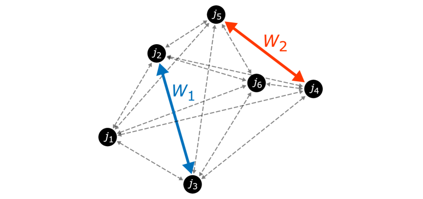
(a) Graph representation

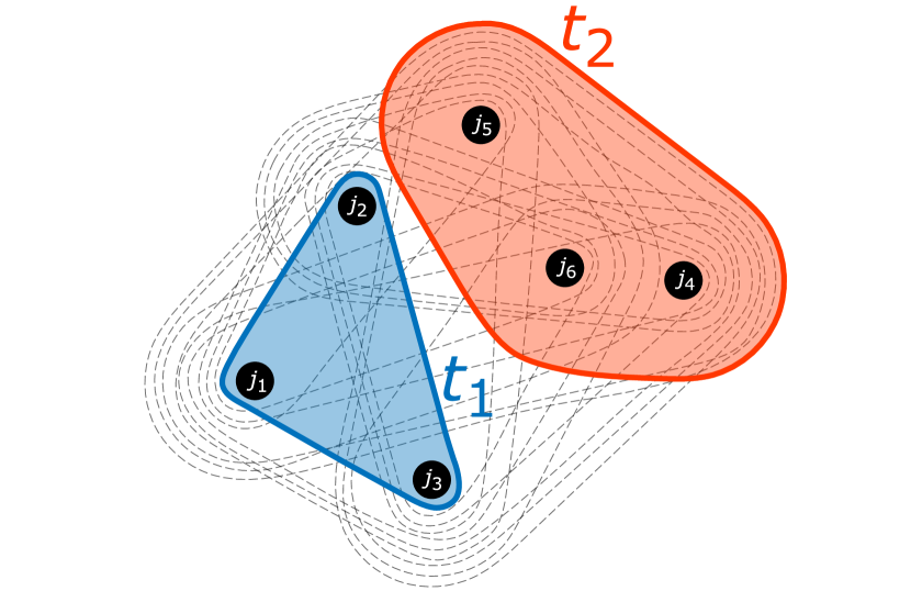
(b) Hypergraph representation

Figure 2: Illustrations of an event in (a) graph and (b) hypergraph representations. Edges and hyperedges shown in grey dashed lines are the false particle candidates in the reconstruction. The coloured edges and hyperedges portray the true parent particles of nodes that they connect.

The graph representation of an event with six final-state jets is shown in Fig 2(a). In this representation, the decay products of each $W$ boson constitute two distinct nodes: accounting for the direction of the edges, there exist precisely two edges in $E$ representing each true $W$ boson candidate. The edges representing each $W$ boson can be learned using the message-passing technique, which is introduced further in Section 3, and whose specific implementation in HyPER is described in Appendix A.2. The task of reconstructing $W$ bosons — and indeed any two-body decay — is an edge classification task. The correct edge candidates are shown by the colored arrows in Fig 2(a).

In the graph representation, there are three nodes that correspond to the decay products of each top quark. However, a digraph lacks representation of relations between more than two nodes. Top quarks, therefore, cannot be effectively represented using a conventional graph. To address this challenge and ultimately reconstruct top quark pairs, HyPER introduces a set of generalized edges called hyperedges, $\mathcal{E}=\{\tilde{E}_{1},\tilde{E}_{2},\dots,\tilde{E}_{M}\}$, which are sets containing arbitrary numbers of nodes. Specifying identical nodes to the digraph representation, the corresponding hypergraph is defined as $H=(V,\mathcal{E})$.

Top quark candidates can be represented by hyperedges which are comprised of exactly three nodes:

$$\tilde{E}_{m}\in\{\{i,j,k\}\;|\;i,j,k\in V\;\mathrm{and}\;i\neq j\neq k\},$$ (3)

where $m=1,2,\dots,M$, and $M$ is the number of hyperedges. Utilizing the hidden relational information between pairs of nodes learned during the message-passing, HyPER constructs hyperedge embeddings, $\mathbf{\tilde{e}}_{m}$, and subsequently classifies the hyperedges representing the top quarks. We call the combined use of message-passing on graphs with hyperedge classification blended graph-hypergraph representation learning.

For an event with a jet multiplicity of six, there are 20 combinations of three jets, leading in principle to 20 candidate top quark hyperedges. This structure is shown in Fig. 2(b), where the dashed grey lines represent all possible 3-node hyperedges. The classified $t_{1}$ and $t_{2}$ candidates are given by the blue- and orange-shaded hyperedges respectively. The number of candidate hyperedges could be reduced by imposing certain restrictions. An example would be requiring that each candidate hyperedge contain a node corresponding to a $b$-tagged jet. As $b$-tagging algorithms are not 100% accurate, we choose to implement HyPER without posing any additional requirements on the constituents of the hyperedges.

III The HyPER Network

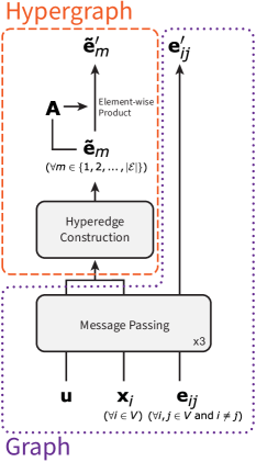
Figure 3: Network architecture of HyPER. HyPER uses a mixed graph-hypergraph representation. The network components that operate on the graph are enclosed within the purple dotted line, and the components that operate on the hypergraph are enclosed within the orange dashed line.

We implement the blended graph-hypergraph approach outlined in Section II through HyPER, whose basic architecture is sketched in Fig 3. HyPER embeds the kinematic information of an event’s final state in the conventional graph structure specified in Eq. 2. These feature-embedded graphs are passed into a message-passing neural network, which is comprised of multiple layers of message-passing aggregation operations. Message-passing explores the graph feature space by exchanging information between neighboring nodes. Each message-passing layer leverages relational information encoded in the graph structure to update the node, edge, and global feature vectors. The message-passing architecture is detailed in Appendix A.2. Each message-passing layer is enumerated with index $t$, with $t=0$ indicating the initial inputs prior to the first message-passing phase. After the final message-passing operation, $t=T$, the updated attribute vectors $\mathbf{u}^{(T)},\mathbf{x}^{(T)}_{i}\in\mathbb{R}^{S}$ ($\forall i\in V$) have a dimension of $S$; they are preserved and carried on to the top quark reconstruction stage. The final edge attributes $e_{ij}^{(T)}\in\mathbb{R}$ are used to reconstruct $W$ bosons.

III.1 Hypergraph: reconstruction of the top quarks

Using a set of pre-defined hyperedges $\mathcal{E}$, according to Eq. 3, HyPER constructs hyperedge features by incorporating node and edge attributes inherited from the messages-passing using an aggregation operator:

$$\mathbf{\tilde{e}}_{m}=\bigoplus_{l\in\tilde{E}_{m}}\Big{(}\textrm{\scriptsize MLP}\left(\mathbf{x}_{l},\mathbf{u}\right)\Big{)},\quad\forall\tilde{E}_{m}\in\mathcal{E},$$ (4)

where $l$ is the index of a node connected by the hyperedge $m$, and MLP is a Multilayer Perceptron (MLP). Eq. 4 maps the incoming features to a $D$-dimensional hyperedge embedding: $\mathbf{\tilde{e}}_{m}\in\mathbb{R}^{D}$.

We seek to assign each hyperedge a score representing the probability that it corresponds to a true top quark. This is achieved by processing the hyperedge embeddings with a hyperedge layer which reduces the dimensionality while capturing the most salient features. The hyperedge layer is defined as

$$\tilde{e}^{\prime}_{m}=\textrm{\scriptsize Sigmoid}\Bigg{(}\textrm{\scriptsize MLP}\Bigg{[}\mathbf{A}_{m}\circ\textrm{\scriptsize ReLU}\left(\mathbf{\tilde{e}}_{m}\mathbf{W}^{\mathrm{T}}\right),\mathbf{\tilde{e}}_{m}\Bigg{]}\Bigg{)},$$ (5)

where $\mathbf{W}\in\mathbb{R}^{D\times D}$ is a learnable weight matrix that linearly transforms hyperedge features. Nonlinearity is introduced to the transformed features using a rectified linear unit [6] (ReLU).
Inspired by attention mechanisms [veličković2018graph], a set of coefficient vectors,

$$\mathbf{A}_{m}=(A_{1m},A_{2m},\dots,A_{Dm}),$$ (6)

is derived from the incoming hyperedge features, with each coefficient given by

$$A_{dm}=\frac{\exp\left(\tilde{e}_{dm}\right)}{\sum_{m=0}^{M}\exp\left(\tilde{e}_{dm}\right)},$$ (7)

where $A_{dm}\in[0,1]$ represents the importance of a feature $d\in\{1,2,\dots,D\}$ to a given top quark candidate $m$. Weighted hyperedge attributes are produced by applying the derived coefficient vectors to their corresponding, transformed hyperedge features using the element-wise product, as denoted by $\circ$ in Eq. 5. Together with the unweighted hyperedge features, they are processed by an MLP for dimensionality reduction, and subsequently transformed with a logistic function, Sigmoid, producing a soft probability: $\tilde{e}^{\prime}_{m}\in[0,1]$. It represents the probability of hyperedge $m$ portraying an actual top quark. Top quark pairs are reconstructed by selecting the two independent, highest-scoring hyperedges.

III.2 Graph: identification of the $W$ boson

The graph edge attributes obtained from the message-passing, $e_{ij}^{(T)}$, are transformed with the Sigmoid function, yielding a probability that the edges corresponds to the actual $W$ boson. Since the ordering of the decays is invariant in the context of reconstruction, edges with the same endpoints are combined using a permutation invariant function:

$$e^{\prime}_{ij}=\textrm{mean}\left(e_{j\rightarrow i},e_{i\rightarrow j}\right),$$ (8)

thus, $e^{\prime}_{ij}=e^{\prime}_{ji}$. The reconstruction of $W$ bosons then follows the reconstruction of the top quarks: if $\tilde{E}_{t}$ is the hyperedge representing the selected top quark, all permissible $W$ boson candidates exist as edges whose nodes are contained in $\tilde{E}_{t}$. The highest-scoring edge which meets this requirement,

$$\max\left(e^{\prime}_{ij}\right),\;\;{i,j\in\tilde{E}_{t}},\;i\neq j,$$ (9)

is the reconstructed $W$ boson.

III.3 Training

The graph and hypergraph components of HyPER are combined, following the introduction of the loss function:

$$\mathcal{L}=\alpha\mathcal{L}_{\textrm{BCE}}(\mathcal{E},\hat{\mathcal{E}})+(1-\alpha)\mathcal{L}_{\textrm{BCE}}(E,\hat{E}),$$ (10)

where $\mathcal{L}_{\textrm{BCE}}$ is the binary cross-entropy (BCE) loss, and $\hat{\mathcal{E}}$ and $\hat{E}$ denote labeled hyperedges and graph edges, respectively. The hyperparameter $\alpha\in[0,1]$ is introduced to adjust the training importance between graph and hypergraph components. Mini-batching, where multiple graphs are aggregated to improve computational efficiency, is employed. To maximize the event reconstruction efficiency, we compute the loss for each event; the loss of each mini-batch is the average loss across all events within that mini-batch.

The network is trained with the Adam optimizer [7]. Tuning is performed, with the details of the tuning procedure and a summary of the chosen hyperparameters described in Appendix A.4. Specifically, the message-passing embedding dimension is set to $S=64$, the dimension of the hyperedge embedding to $D=128$, and the parameter $\alpha$ to 0.8. Individual tuning is recommended for each individual HyPER use case.

Table 1: Reconstruction performance of HyPER, SPANet and Topograph evaluated by the event efficiency ($\varepsilon_{t\bar{t}}$) and top quark efficiency ($\varepsilon_{t}$) calculated in different jet multiplicity regions.

	$\varepsilon_{t\bar{t}}$			$\varepsilon_{t}$
Jet Multiplicity	HyPER	SPANet	Topograph	HyPER	SPANet	Topograph
$=6$	$0.813\pm 0.002$	$0.801\pm 0.002$	$0.805\pm 0.002$	$0.663\pm 0.001$	$0.667\pm 0.001$	$0.658\pm 0.001$
$=7$	$0.666\pm 0.002$	$0.654\pm 0.002$	$0.649\pm 0.002$	$0.651\pm 0.001$	$0.649\pm 0.001$	$0.638\pm 0.001$
$\geq 8$	$0.504\pm 0.003$	$0.487\pm 0.003$	$0.472\pm 0.003$	$0.595\pm 0.001$	$0.586\pm 0.001$	$0.573\pm 0.001$
Inclusive	$0.664\pm 0.001$	$0.651\pm 0.001$	$0.645\pm 0.001$	$0.641\pm 0.001$	$0.640\pm 0.001$	$0.629\pm 0.001$

IV Simulation

A total of 60 million $t\bar{t}$ events are simulated at a center of mass energy of $\sqrt{s}=13$ TeV. Their matrix elements (ME) are generated using MadGraph5_aMC@NLO [8] (v2.9.16) at next-to-leading order (NLO) in QCD, interfaced to the five-flavour scheme NNPDF3.0nlo parton distribution function (PDF) set [9]. The top quark mass is set to $m_{t}=172.5$ GeV. We consider only hadronic decays of the top quarks, and these decays are modeled using MadSpin [10]. The factorization ($\mu_{F}$) and renormalization scales ($\mu_{R}$) are set to $\mu_{F}=\mu_{R}=m_{T}$, where $m_{T}=\sqrt{m_{t}^{2}+0.5\times(p_{T}^{2}(t)+p_{T}^{2}(\bar{t}))}$ is the transverse mass of the top quark. Events are matched to Pythia8 [bierlich22] (v8.306) to simulate parton shower evolution, hadronization, and multi-parton interactions. The simulation of the detector response is performed by Delphes [11] (v3.5.0) with a parametrization corresponding to the ATLAS detector [12]. Jets are defined using the anti-$k_{t}$ [13] jet finding algorithm, as implemented in FastJet [14] (v3.4.0), with the cone radius parameter set to $R=0.4$. We impose a selection which mimics that which would be imposed on real data: reconstructed jets must have a minimum $p_{T}$ of 25 GeV and an absolute pseudo-rapidity within the ATLAS detector limit of $|\eta|<2.5$. Jets containing b-hadrons ($b$-jets) are tagged using a $p_{T}$-dependent tagging efficiency (mis-identification rate) based on [15].

Supervised learning requires a training sample where the desired outputs are labeled. In the context of this study, the true origin of each jet is established using a generic $\Delta R$ matching scheme. The matching procedure first identifies the outgoing hard particles of the ME using the generator history, then calculates the angular distance $\Delta R=\sqrt{\Delta\eta^{2}+\Delta\phi^{2}}$ between each pair of clustered jets and hard particles. A jet is considered to have originated from a particle if the angular distance between them satisfies $\Delta R<0.4$. Only the closest jet in a particle’s vicinity is considered to avoid multiple jets being matched to the same particle.

Of the events which pass the kinematic selections, 90% are allocated for model training, with 5% used for model validation and 5% for model performance evaluation. We impose pre-selection requirements corresponding to an all-hadronic $t\bar{t}$ selection which would be imposed on real collider data. This selection requires each generated event to contain at least six jets, of which at least two must be considered $b$-tagged. A particle is considered identifiable if all of its decay products have been matched using the $\Delta R$ truth-matching procedure. Events are also required to contain at least one identifiable $W$ boson. After the pre-selection, 7,921,299 events remain for training, 439,692 for validation, and 440,069 for testing. Imposing the condition that both top quarks should be identifiable reduces the number of events to 2,116,231 for training, 117,487 for validation, and 116,960 for testing. These events are called fully matched events, in contrast to partially matched events which have one or more missing jet labels. The highest jet multiplicity recorded in a single event is 20. The full dataset is accessible at [16].

V Results

HyPER is benchmarked against SPANet [2, 3] (v2.2) and Topograph [4]. The SPANet model hyper-parameters are set to match the ones prescribed in [3, 3]. Topograph is configured using recommended settings provided in [4]. All three networks are trained using the same training and validation datasets defined in Section IV. The three networks have different training strategies for dealing with partially matched events, and missing labels could potentially affect the accuracy of the models [17, 18]. We present the resulst of the three networks trained on fully matched events, and provide performance comparison for models trained on partially matched events in Appendix B.

Table 2: Performance of HyPER, SPANet and Topographs are compared for $W$ boson reconstruction.

	$\varepsilon_{W}$
Jet Multiplicity	HyPER	SPANet	Topographs
$=6$	$0.697\pm 0.001$	$0.688\pm 0.001$	$0.683\pm 0.001$
$=7$	$0.681\pm 0.001$	$0.671\pm 0.001$	$0.662\pm 0.001$
$\geq 8$	$0.623\pm 0.001$	$0.608\pm 0.001$	$0.594\pm 0.001$
Inclusive	$0.673\pm 0.001$	$0.662\pm 0.001$	$0.653\pm 0.001$

Focusing on models trained on fully matched events, we apply each fully converged network model to the testing dataset. To assess the performance of different networks, we compare their reconstruction results with the truth labels. We introduce two metrics to quantify the performance: per-top efficiency, $\varepsilon_{t}=N_{t}^{\text{correct}}/N_{t}^{\text{identifiable}}$, represents the fraction of top quarks successfully reconstructed from all identifiable ones; per-event efficiency, $\varepsilon_{t\bar{t}}=N_{t\bar{t}}^{\text{correct}}/N_{t\bar{t}}^{\text{FM}}$, is the fraction of fully matched events with both top quarks correctly reconstructed out of all fully matched events. A top quark is considered correctly reconstructed when all its final states are correctly assigned, ignoring the permutations of the two jets originating from the $W$ boson. A correctly reconstructed event has both top quarks successfully reconstructed, disregarding the ordering of the two. The two performance metrics are computed for all three networks in different jet multiplicity regions, and presented in Table 1. Similarly, the per-$W$ efficiency metric, $\varepsilon_{W}$, represents the fraction of $W$ bosons successfully reconstructed from all identifiable ones. This metric is presented for the three networks in Table 2. We choose to define $\varepsilon_{t}$ and $\varepsilon_{W}$ for all identifiable top quarks and $W$ bosons, regardless of whether the event itself is fully matched or partially matched. We provide analogous efficiencies, defined only for fully matched events, in Appendix C, for direct comparison with the efficiencies presented in [3].

All statistical uncertainties are estimated using the standard expression for the statistical error on efficiencies. The observed differences between the three networks are relatively small compared to the size of the testing set, which contains 116,960 fully matched events and 525,014 identifiable top quarks. Consequently, the estimated statistical uncertainties in each jet multiplicity region are practically identical for all networks within the limits of rounding precision.

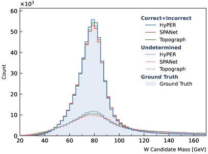
(a)	(b)

Figure 4: Invariant mass distributions of reconstructed (a) top quarks and (b) $W$ bosons, shown in combined correct-incorrect (solid) and undetermined (dotted) categories. They are compared to the truth mass distributions (shaded light-blue) obtained using jet assignment labels.

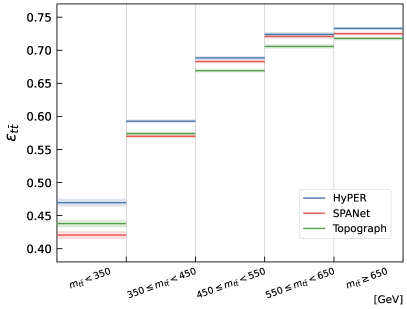
Figure 5: Event reconstruction efficiencies of HyPER, SPANet and Topograph, calculated in various truth $t\bar{t}$ invariant mass ($m_{t\bar{t}}$) regions.

While all three networks exhibit a reduction in performance as jet multiplicity increases, HyPER delivers a marginally higher $\varepsilon_{t\bar{t}}$ than its counterparts in all jet multiplicity regions. This translates into a better inclusive event efficiency of 0.664, compared to SPANet (0.651) and Topograph (0.645). For top quark efficiency, $\varepsilon_{t}$, SPANet performs slightly better than HyPER in the lowest jet multiplicity region. HyPER remediates its inclusive $\varepsilon_{t}$ with better performance in higher multiplicity regions, reconstructing 64.1% of identifiable top quarks in the inclusive region. HyPER also performs marginally better in the reconstruction of $W$ bosons compared to the other techniques, as quantified by per-$W$ efficiency $\varepsilon_{W}$. The differences in performance between the three networks are less pronounced than previous comparisons of SPANet and Topograph to the historic $\chi^{2}$ method [2, 3, 4]. Nevertheless, with a network size of 345K, HyPER has shown comparable performance when pitted against the SPANet and Topograph techniques, which have network sizes of 10.7M and 6.5M, respectively. The impact of network size on possible over-training is estimated by considering the difference in model performance when evaluated on the training dataset and the testing dataset. This study is presented in Appendix D, including a scenario where all three models are re-trained on a smaller dataset. HyPER is shown to be the most robust under reductions in training dataset size.

Using the truth jet assignments, each reconstructed top quark or $W$ boson can be tagged with one of the three orthogonal classes: correct, incorrect, and undetermined. They represent cases where the top quark (or $W$ boson) is correctly reconstructed, incorrectly reconstructed, or undetermined due to missing truth label(s), respectively. A candidate that falls into the correct or incorrect category has by definition an associated truth counterpart. A direct comparison can be drawn between the ground truth and the reconstructed invariant mass spectrum of particles which fall into either the correct or incorrect categories. This comparison is shown in Fig. 4. All three networks successfully recover the top quark and $W$ boson invariant mass peaks, generally retaining the shape of the truth kinematics that the networks were trained upon. Candidates classified under the undetermined category have no truth counterpart due to the presence of one or more unmatched jets. As a consequence, undetermined events cannot be used to assess network performance. However, the invariant mass distributions for the set of undetermined events shows agreement with the shapes of the combined correct and incorrect distributions, peaking around the expected top quark and $W$ boson masses.

To investigate network accuracy across the kinematic phase-space, the event efficiency, $\varepsilon_{t\bar{t}}$, is calculated in various truth invariant mass bins of the $t\bar{t}$ system, as illustrated in Fig. 5. All three methods exhibit an increase in $\varepsilon_{{t}\bar{t}}$ as harder top quark pairs are produced. The two reference methods achieve similar inclusive event efficiency by prioritizing either lower or higher $m_{t\bar{t}}$ bins: Topograph provides better efficiencies in lower $m_{t\bar{t}}$ bins, and SPANet overtakes Topograph in the higher $t\bar{t}$ mass regions. HyPER displays the best event efficiencies across the board, in particular providing better reconstruction for events around and below the $t\bar{t}$ production threshold.

VI Conclusions

In this paper, we have introduced HyPER, a novel methodology that combines graph and hypergraph representation learning to reconstruct particles in collider events with complex final states. We presented benchmark tests against two existing state-of-the-art methods, SPANet and Topograph, focusing on reconstructing top quarks and $W$ bosons in the all-hadronic $t\bar{t}$ channel. The HyPER approach yields competitive results, reconstructing 66.4% of the fully matched events, compared to the 65.1% achieved by SPANet and 64.5% by Topograph, with a network architecture that contains a factor of 20 less parameters. HyPER also demonstrates comparatively higher performance in all $t\bar{t}$ invariant mass regions.

A unique feature of HyPER is its blended graph-hypergraph representation of events, a new development in kinematic reconstruction problems. Edge and hyperedge classification were used to reconstruct $W$ bosons and top quarks, respectively, but hyperedges can represent candidate particles which decay into an arbitrary number of final states. In principle, this facilitates the reconstruction of any short-lived SM or BSM particle. The versatility of this approach, which can be applied to arbitrarily complex collider processes, should allow for the effective reconstruction of a wide variety of physics processes. For instance, the associated production of a top quark pair and Higgs boson, $t\bar{t}H$, can be represented using a graph and a hypergraph whose structures are identical to a $t\bar{t}$ event with an additional target edge label specified for the Higgs boson. Ongoing work also considers the simultaneous reconstruction of final-state neutrino kinematics, with the aim of reconstructing four-top production events in multiple decay channels.

Many experimental measurements require both the reconstruction of heavy states and the classification of the production process, the latter being used to separate a signal from potential backgrounds. These two tasks are often performed by separate multivariate tools. Similarly to approaches taken by SPANet and Topograph, the edge and hyperedge outputs of HyPER can be used to construct discriminants that can serve as inputs to downstream classification networks. However, by taking advantage of pre-existing message-passing operations, HyPER can, in principle, be expanded to perform event classification while simultaneously reconstructing particles. This can be achieved by incorporating an additional loss term that utilizes the output of the global graph attributes, $\mathbf{u}$, whose inherent representation of graph-wise information makes it ideal for extracting event-level properties. Despite the introduction of a supplementary classification task, no additional MLPs are introduced, thus HyPER will remain parameter-efficient.

Appendix A Additional information on HyPER

In this section, we describe some of the fundamental components of HyPER, including network inputs, mathematical formulations of the message-passing operation, and the general design of the MLP(s). We also provide a list of optimized hyperparameters essential for recreating the results presented.

A.1 Graph input kinematics

The parameters ${p_{T}}_{i}$ and $E_{i}$ correspond to the transverse momentum and energy of the $i^{th}$ jet, respectively. Angular terms $\eta_{i}$ and $\phi_{i}$ correspond to the pseudorapidity and azimuth angle in the transverse plane, as defined with respect to the standard ATLAS coordinate system; $\Delta\eta_{ij},\Delta\phi_{ij}$ are the corresponding angular separations between the $i^{th}$ and $j^{th}$ jets. The term $\Delta R_{ij}$ represents the Euclidean separation in the $\eta$–$\phi$ plane, as given by $\sqrt{\Delta\eta^{2}+\Delta\phi^{2}}$. The boolean $b\textrm{-tag}_{i}$ labels whether the jet is $b$-tagged. The term $M_{ij}$ is the invariant mass of the $ij$ jet pair: $(p_{i}+p_{j})^{\mu}\cdot(p_{i}+p_{j})_{\mu}$, where $p$ is the four-momentum of each jet. The global terms $N_{\textrm{jets}}$ and $N_{b\textrm{-tagged}}$ denote the total number of jets in the event and the number that are $b$-tagged, respectively. Additionally, a node-type label, $K$, is included to distinguish different types of final states. Values of 1, -1, -2, and 0 corresponding to jet, electron, muon, and missing energy, respectively. As we only consider an all-hadronic final state, $K_{i}=1\>(\forall i\in V)$; the inclusion of this parameter allows HyPER to be generalized to a wider class of final states in future work.

A.2 Message-passing

Message-passing is a convolution operation that has been generalized to operate on non-Euclidean domains, such as graph-structured data [19, 20]. The message-passing technique used in HyPER is adopted from [19, 21, 22, 20]. A complete message-passing layer consists of three mathematical operations that update edge, node, and global attributes.

At an initial time-step $t$, the message-passing process begins by gathering all available features in a graph and updating the edges according to an aggregation operation

$$\mathbf{e}_{ij}^{(t+1)}=\textrm{\scriptsize MLP}_{\mathbf{e}}^{(t)}\left(\mathbf{x}_{i}^{(t)},\mathbf{x}_{j}^{(t)},\mathbf{e}_{ij}^{(t)},\mathbf{u}^{(t)}\right),$$ (11)

where $i$ and $j$ are two adjacent nodes. A message, $\mathbf{m}_{ij}$, is then calculated for each updated edge with a message function defined as

$$\mathbf{m}_{ij}^{(t)}\equiv\mathbf{m}_{j\rightarrow i}^{(t)}=\textrm{\scriptsize MLP}_{\mathbf{m}}^{(t)}\left(\mathbf{x}_{i}^{(t)},\mathbf{x}_{j}^{(t)},\mathbf{e}_{ij}^{(t+1)}\right).$$ (12)

Messages are signed, $\mathbf{m}_{ij}\neq\mathbf{m}_{ji}$: they have identical directions to the edges they are carried by. The notation $j\rightarrow i$ indicates the source and recipient nodes of the message, respectively. Once the recipient node $i$ has received all the messages from its direct neighbors, these messages are then summarized, updating the recipient node to its next state as follows:

$$\mathbf{x}_{i}^{(t+1)}=\textrm{\scriptsize MLP}_{\mathbf{x}}^{(t)}\left[\mathbf{x}_{i}^{(t)},\mathbf{u}^{(t)},\underset{{\forall j:\>j\rightarrow i}}{\mathrm{mean}}\left(\mathbf{m}_{ij}^{(t)}\right),\max_{{\forall j:\>j\rightarrow i}}\left(\mathbf{m}_{ij}^{(t)}\right)\right].$$ (13)

The global attribute vector, $\mathbf{u}$, is updated to its next instance by collecting information from updated nodes. This process is formulated as

$$\mathbf{u}^{(t+1)}=\textrm{\scriptsize MLP}_{\mathbf{u}}^{(t)}\left[\mathbf{u}^{(t)},\mathrm{mean}\left(\mathbf{x}_{i}^{(t+1)}\right),\max\left(\mathbf{x}_{i}^{(t+1)}\right)\right].$$ (14)

It concludes a full message-passing layer. The updated states $\mathbf{e}_{ij}^{(t+1)}$, $\mathbf{x}_{i}^{(t+1)}$ and $\mathbf{u}^{(t+1)}$ are used as the inputs for the next message-passing iteration ($t+1$). The Message-passing operation is repeated, taking the outputs of the previous layer as the inputs of the subsequent layer until the number of maximum iterations $T$ is reached. In this study, we have implemented three message-passing layers, ensuring that all objects have exchanged and received crucial information.

A.3 MLP design

Multilayer perceptions are the fundamental building blocks of HyPER. The MLPs used in the HyPER are designed with the same architecture varying only in the dimensionalities of the input and output attribute vectors. Each MLP containing two fully-connected hidden layers, formulated as following

$$\phi(\mathbf{h}_{n},n)=\textrm{\scriptsize Dropout}\Bigg{[}\textrm{\scriptsize ReLU}\Big{(}\mathbf{h}_{n}\mathbf{W}^{\mathrm{T}}_{n}+\mathbf{b}_{n}\Big{)}\Bigg{]},$$ (15)

where $\mathbf{h}_{n}$ is the input attributes of the hidden layer $n$. The dimensionalities of the weight matrices $\mathbf{W}_{n}$ are determined by the input and output dimension of the MLP, which various in different operations. Two activation functions are introduced in Eq. 15: ReLU [6] and Dropout [23]. ReLU is applied to introduce non-linearity. Dropout, a regularization activation function is applied subsequent to the ReLU. It arbitrarily sets a fraction of features to zero during training, which helps prevent overfitting.

A.4 Hyperparameters

A set of optimized hyperparameters used in the study is shown in Table 3. Hyperparameter tuning is performed by the Optuna (v3.4) [24] optimization framework. A sum of 100 HyPER models is tested, corresponding to the 100 sets of hyperparameters sampled by Optuna. Each model is trained for 10 epochs. Pruning is used for efficient tuning, which terminates unpromising trials at early stages. The training and validation datasets used for tuning are randomly sampled from the primary training dataset; they contain 1M and 50,000 events, respectively.

Table 3: A list of hyperparameters used to setup HyPER for the presented study.

Name	Notation	Value
Number of message-passing iterations	$T$	3
Message dimensionality	$S$	64
Hyperedge dimensionality	$D$	128
Learning rate	$\gamma$	0.0003
Loss mixing	$\alpha$	0.8
Dropout	$p$	0.01

Table 4: Performance of HyPER, SPANet and Topograph in reconstructing individual top quarks and $W$ bosons in fully matched events.

	$\varepsilon_{t}^{\text{FM}}$			$\varepsilon_{W}^{\text{FM}}$
Jet Multiplicity	HyPER	SPANet	Topograph	HyPER	SPANet	Topograph
$=6$	$0.851\pm 0.001$	$0.838\pm 0.001$	$0.843\pm 0.001$	$0.891\pm 0.001$	$0.881\pm 0.001$	$0.884\pm 0.001$
$=7$	$0.764\pm 0.002$	$0.751\pm 0.002$	$0.750\pm 0.002$	$0.811\pm 0.001$	$0.798\pm 0.001$	$0.797\pm 0.001$
$\geq 8$	$0.660\pm 0.003$	$0.644\pm 0.002$	$0.636\pm 0.002$	$0.713\pm 0.002$	$0.695\pm 0.002$	$0.685\pm 0.002$
Inclusive	$0.760\pm 0.001$	$0.746\pm 0.001$	$0.745\pm 0.001$	$0.807\pm 0.001$	$0.793\pm 0.001$	$0.791\pm 0.001$

Appendix B Partial event training

The $\Delta R$ truth-matching scheme often fails to associate jets to their parent particles, resulting in missing jet origin labels. These events are tagged as partially matched. SPANet can be trained on events with at least one identifiable top quark, and for HyPER and Topograph, at least one identifiable $W$ boson is required. For HyPER, in the case where an event has no identifiable top quarks due to two missing $b$-quark labels, $\alpha$ in Eq. 10 is set to zero, such that only the loss of the $W$ boson is considered. We train all three networks on the training and validation datasets defined in Section IV and conduct performance evaluation on the testing dataset. Network performance is assessed with the event efficiency ($\varepsilon_{t\bar{t}}$) and the top quark efficiency ($\varepsilon_{t}$); results are shown in Table 5.

Table 5: Event efficiency ($\varepsilon_{t\bar{t}}$) and the per-top quark efficiency ($\varepsilon_{t}$) evaluated in various jet multiplicity regions using partially trained HyPER, SPANet, and Topograph models.

	$\varepsilon_{t\bar{t}}$
Jet Multiplicity	HyPER	SPANet	Topograph
$=6$	$0.792\pm 0.002$	$0.808\pm 0.002$	$0.787\pm 0.002$
$=7$	$0.656\pm 0.002$	$0.667\pm 0.002$	$0.632\pm 0.002$
$\geq 8$	$0.503\pm 0.003$	$0.503\pm 0.003$	$0.462\pm 0.003$
Inclusive	$0.653\pm 0.001$	$0.663\pm 0.001$	$0.631\pm 0.001$
	$\varepsilon_{t}$
Jet Multiplicity	HyPER	SPANet	Topograph
$=6$	$0.703\pm 0.001$	$0.698\pm 0.001$	$0.677\pm 0.001$
$=7$	$0.669\pm 0.001$	$0.668\pm 0.001$	$0.644\pm 0.001$
$\geq 8$	$0.605\pm 0.001$	$0.601\pm 0.001$	$0.570\pm 0.001$
Inclusive	$0.667\pm 0.001$	$0.663\pm 0.001$	$0.638\pm 0.001$

All three models exhibit increased $\varepsilon_{t}$ compared to models trained with fully matched events. This is due to the significantly expanded training set, which allows the networks to access more identifiable top quarks during training. SPANet has a slightly improved $\varepsilon_{t\bar{t}}$ upon training with fully matched events, while the two GNN-based networks, HyPER and Topograph, have minor reductions in performance. Trained using partially matched events, HyPER and SPANet show comparable per-event and per-top quark efficiencies, and show a slight improvement over the corresponding Topograph efficiencies.

Though not tested here, HyPER’s performance could potentially be improved by scaling up the dimensionalities of message and hyperedge attribute vectors.

Appendix C Fully matched efficiencies

Per-top efficiency $\varepsilon_{t}$ and per-$W$ efficiency $\varepsilon_{W}$ are defined in Section V as the ratio of correctly reconstructed particles to all identifiable particles of that type, regardless of whether the event is fully matched or partially matched. The related metrics $\varepsilon_{t}^{\text{FM}}$ and $\varepsilon_{W}^{\text{FM}}$ are the related efficiencies defined only for fully matched events. This provides direct comparison with [3]. The results are tabulated in Table 4. Each metric is larger compared to the efficiencies computed for fully matched and partially matched events. Results are similar for each network in all jet multiplicity regions, with HyPER displaying the highest efficiencies in all categories.

Appendix D Overtraining test

With a total network size of 345K, HyPER demonstrates superior parameter efficiency, achieving performance comparable to SPANet (10.7M) and Topograph (6.5M). Larger networks can be susceptible to overtraining. This is quantified by considering the difference in a model’s performance when evaluated on the training dataset and on the testing dataset. It is common for models to perform slightly better when evaluated on the training dataset. However, a strong indicator of an overtrained model is one where the difference in performance between evaluation on the training and testing datasets is large.

Using performance metric $\varepsilon_{t\bar{t}}$, the possibility of overtraining is assessed for HyPER, SPANet and Topograph. The training dataset (which contains 2,116,231 fully matched events) is sampled randomly to produce a new dataset of equivalent size to the testing dataset. The models, as derived from training on the full training dataset, are then applied to this new subset of the training dataset. The values of $\varepsilon_{t\bar{t}}^{\text{test}}$ are given in Table 6, along with the difference between the training and testing scores i.e. $\Delta=\varepsilon_{t\bar{t}}^{\text{train}}-\varepsilon_{t\bar{t}}^{\text{test}}$, where ‘train’ corresponds to evaluation on the smaller training dataset. We observe that the differences in $\varepsilon_{t\bar{t}}$ between the training and testing datasets are small. This indicates that there is minimal overtraining of each network, thus each network generalizes well to new data.

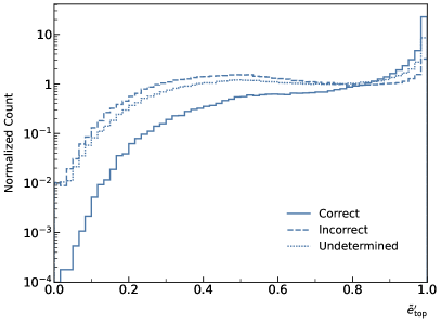
(a)	(b)

Figure 6: HyPER output distributions of reconstructed (a) top quarks, $\tilde{e}^{\prime}_{\mathrm{top}}$, and (b) $W$ bosons, $e^{\prime}_{W}$.

Many experimental measurements do not have access to large simulated samples for network training. Examples include heavy Higgs searches which require simulation samples generated at a large number of different heavy Higgs mass points. In such cases, each sample can have as little as several hundred thousand generated events. We therefore consider the question of how the various networks perform when trained on smaller datasets. We re-train each network on a training set composed of 439,598 events, of which 117,812 are fully matched. The “Reduced Dataset” column in Table 6 presents the corresponding results for these re-trained models. In this case, the differences between evaluation on the training and testing datasets are larger. The difference $\Delta$ for HyPER is far smaller than the other networks, indicating that it exhibits less overtraining than SPANet or Topograph when trained on a reduced dataset. The parameter-efficient HyPER is therefore more robust when used on training datasets of limited size.

Table 6: Reconstruction performance for the full model, trained on all fully matched events, and a comparison model trained on a reduced dataset of 100K events. Performance as evaluated on the testing dataset is given by $\varepsilon_{t\bar{t}}^{\mathrm{test}}$, and $\Delta$ gives the difference in $\varepsilon_{t\bar{t}}$ between evaluation on the testing and training datasets. The statistical uncertainty is identical for each of the three networks.

	Original Dataset		Reduced Dataset
Network	$\varepsilon_{t\bar{t}}^{\mathrm{test}}$	$\Delta$	$\varepsilon_{t\bar{t}}^{\mathrm{test}}$	$\Delta$
HyPER	$0.664$	$0.005$	$0.607$	$0.013$
SPANet	$0.651$	$0.025$	$0.544$	$0.098$
Topograph	$0.645$	$0.002$	$0.602$	$0.035$
Uncertainty	$\pm 0.001$	$\pm 0.002$	$\pm 0.001$	$\pm 0.002$

Appendix E HyPER outputs

The reconstruction procedure selects two independent highest-scoring hyperedges to form top quark candidates. An enclosed highest-scoring graph edge is chosen for each selected hyperedge as its corresponding $W$ candidate. We record the scores for the reconstructed top quarks and $W$-bosons, denoted by $\tilde{e}^{\prime}_{\textrm{top}}$ and $e^{\prime}_{W}$ respectively. The two distributions are shown in Fig. 6 (a) and Fig. 6 (b), subdivided into “correct”, “incorrect”, and “undetermined” categories as before. The scores $\tilde{e}^{\prime}_{\textrm{top}}$ and $e^{\prime}_{W}$ demonstrate reasonable separation between the three categories.

We propose that these scores could be used as discriminants for enhancing the efficiency of correctly reconstructed particles. Though not investigated in this paper, one could impose a cut on $\tilde{e}^{\prime}_{\textrm{top}}$ and $e^{\prime}_{W}$ to increase the confidence that the reconstructed objects do correspond to the true particles. For instance, one could require that both top quarks and $W$ bosons in an event must pass the selection requirements $\tilde{e}^{\prime}_{\textrm{top}}>0.8$ and $e^{\prime}_{W}>0.8$. This region constitutes 46.3% of all fully matched events and has an inclusive event efficiency of $\varepsilon_{t\bar{t}}=0.919$. The optimal performance and statistics can be achieved by fine-tuning of these confidence requirements.

Appendix F Supplementary plots

Figure 7: Per-jet assignment efficiencies of the reconstruction networks visualized using normalized confusion matrices. Each row represents the networks’ predictions of the jet origins, and each column represents the true origins of the jets. The category “Other” corresponds to jets which do not originate from the decay of one of the top quarks. This category sums to greater than unity as more than one additional jet can exist in any event. The matrices are evaluated using the fully matched events. HyPER consistently displays the highest percentage of correctly matched jets.

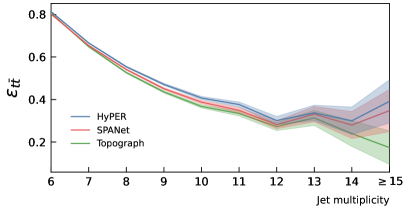
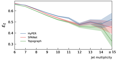
(a)	(b)

Figure 8: Comparison of (a) per-event and (b) per-top efficiencies for HyPER, SPANet, and Topograph in various jet multiplicity regions.

References

- Evans and Bryant [2008] L. Evans and P. Bryant, LHC Machine, JINST 3, S08001.
- Fenton et al. [2022] M. J. Fenton, A. Shmakov, T.-W. Ho, S.-C. Hsu, D. Whiteson, and P. Baldi, Permutationless many-jet event reconstruction with symmetry preserving attention networks, Phys. Rev. D 105, 112008 (2022), arXiv:2010.09206 [hep-ex] .
- Shmakov et al. [2022] A. Shmakov, M. J. Fenton, T.-W. Ho, S.-C. Hsu, D. Whiteson, and P. Baldi, SPANet: Generalized permutationless set assignment for particle physics using symmetry preserving attention, SciPost Phys. 12, 178 (2022), arXiv:2106.03898 [hep-ex] .
- Ehrke et al. [2023] L. Ehrke, J. A. Raine, K. Zoch, M. Guth, and T. Golling, Topological reconstruction of particle physics processes using graph neural networks, Phys. Rev. D 107, 116019 (2023), arXiv:2303.13937 [hep-ph] .
- Aaboud et al. [2017] M. Aaboud et al. (ATLAS), Top-quark mass measurement in the all-hadronic decay channel at TeV with the ATLAS detector, JHEP 09, 118, arXiv:1702.07546 [hep-ex] .
- Agarap [2018] A. F. Agarap, Deep Learning using Rectified Linear Units (ReLU) (2018), arXiv:1803.08375 [cs.NE] .
- Kingma and Ba [2014] D. P. Kingma and J. Ba, Adam: A Method for Stochastic Optimization (2014), arXiv:1412.6980 [cs.LG] .
- Alwall et al. [2014] J. Alwall, R. Frederix, S. Frixione, V. Hirschi, F. Maltoni, O. Mattelaer, H. S. Shao, T. Stelzer, P. Torrielli, and M. Zaro, The automated computation of tree-level and next-to-leading order differential cross sections, and their matching to parton shower simulations, JHEP 07, 079, arXiv:1405.0301 [hep-ph] .
- Ball et al. [2015] R. D. Ball et al. (NNPDF), Parton distributions for the LHC Run II, JHEP 04, 040, arXiv:1410.8849 [hep-ph] .
- Artoisenet et al. [2013] P. Artoisenet, R. Frederix, O. Mattelaer, and R. Rietkerk, Automatic spin-entangled decays of heavy resonances in Monte Carlo simulations, JHEP 03, 015, arXiv:1212.3460 [hep-ph] .
- de Favereau et al. [2014] J. de Favereau, C. Delaere, P. Demin, A. Giammanco, V. Lemaître, A. Mertens, and M. Selvaggi (DELPHES 3), DELPHES 3, A modular framework for fast simulation of a generic collider experiment, JHEP 02, 057, arXiv:1307.6346 [hep-ex] .
- Aad et al. [2008] G. Aad et al. (ATLAS), The ATLAS Experiment at the CERN Large Hadron Collider, JINST 3, S08003.
- Cacciari et al. [2008] M. Cacciari, G. P. Salam, and G. Soyez, The anti- jet clustering algorithm, JHEP 04, 063, arXiv:0802.1189 [hep-ph] .
- Cacciari et al. [2012] M. Cacciari, G. P. Salam, and G. Soyez, FastJet User Manual, Eur. Phys. J. C 72, 1896 (2012), arXiv:1111.6097 [hep-ph] .
- ATLAS Collaboration [2015] ATLAS Collaboration, Expected performance of the ATLAS -tagging algorithms in Run-2, Tech. Rep. (CERN, Geneva, 2015).
- Zhang et al. [2024] Z. Zhang, C. Birch-Sykes, B. Le, Y. Peters, and E. Simpson, Top quark pair production with fully hadronic final states at the LHC, 10.5281/zenodo.10653837 (2024).
- Zhang et al. [2017] C. Zhang, S. Bengio, M. Hardt, B. Recht, and O. Vinyals, Understanding deep learning requires rethinking generalization (2017), arXiv:1611.03530 [cs.LG] .
- Bernhardt et al. [2022] M. Bernhardt et al., Active label cleaning for improved dataset quality under resource constraints, Nature communications 13, 1161 (2022).
- Gilmer et al. [2017] J. Gilmer, S. S. Schoenholz, P. F. Riley, O. Vinyals, and G. E. Dahl, Neural message passing for quantum chemistry (2017), arXiv:1704.01212 [cs.LG] .
- Battaglia et al. [2018] P. W. Battaglia et al., Relational inductive biases, deep learning, and graph networks (2018), arXiv:1806.01261 [cs.LG] .
- Hamrick et al. [2018] J. B. Hamrick, K. R. Allen, V. Bapst, T. Zhu, K. R. McKee, J. B. Tenenbaum, and P. W. Battaglia, Relational inductive bias for physical construction in humans and machines (2018), arXiv:1806.01203 [cs.LG] .
- Sanchez-Gonzalez et al. [2018] A. Sanchez-Gonzalez, N. Heess, J. T. Springenberg, J. Merel, M. Riedmiller, R. Hadsell, and P. Battaglia, Graph networks as learnable physics engines for inference and control (2018), arXiv:1806.01242 [cs.LG] .
- Hinton et al. [2012] G. E. Hinton, N. Srivastava, A. Krizhevsky, I. Sutskever, and R. R. Salakhutdinov, Improving neural networks by preventing co-adaptation of feature detectors, arXiv e-prints (2012), arXiv:1207.0580 [cs.NE] .
- Akiba et al. [2019] T. Akiba, S. Sano, T. Yanase, T. Ohta, and M. Koyama, Optuna: A next-generation hyperparameter optimization framework, in Proceedings of the 25th ACM SIGKDD International Conference on Knowledge Discovery and Data Mining (2019).