Tracking Changing Probabilities via Dynamic Learners

Abstract

Consider a predictor, a learner, whose input is a stream of discrete items. The predictor’s task, at every time point, is probabilistic multiclass prediction, i.e. to predict which item may occur next by outputting zero or more candidate items, each with a probability, after which the actual item is revealed and the predictor learns from this observation. To output probabilities, the predictor keeps track of the proportions of the items it has seen. The predictor has constant (limited) space and we seek efficient prediction and update techniques: The stream is unbounded, the set of items is unknown to the predictor and their totality can also grow unbounded. Moreover, there is non-stationarity: the underlying frequencies of items may change, substantially, from time to time. For instance, new items may start appearing and a few currently frequent items may cease to occur again. The predictor, being space-bounded, need only provide probabilities for those items with (currently) sufficiently high frequency, i.e. the salient items. This problem is motivated in the setting of prediction games, a self-supervised learning regime where concepts serve as both the predictors and the predictands, and the set of concepts grows over time, resulting in non-stationarities as new concepts are generated and used. We develop moving average techniques designed to respond to such non-stationarities in a timely manner, and explore their properties. One is a simple technique based on queuing of count snapshots, and another is a combination of queuing together with an extended version of sparse EMA. The latter combination supports predictand-specific dynamic learning rates. We find that this flexibility allows for a more accurate and timely convergence.

"Occasionally, a new knot of significations is formed.. and our natural powers suddenly
                merge with a richer signification.”     Maurice Merleau-Ponty [33]

Keywords Learning and Development  $\cdot$ Developmental Non-Stationarity  $\cdot$ Online Learning  $\cdot$ Multiclass Prediction  $\cdot$ Probabilistic Prediction  $\cdot$ Categorical Distributions  $\cdot$ Changing Probabilities  $\cdot$ Sparse Moving Averages  $\cdot$ Dynamic Learning Rates  $\cdot$ Stability vs Plasticity  $\cdot$ Probability Reliability  $\cdot$ Lifelong Learning  $\cdot$ Prediction Games

1 Introduction

The external world is ever changing, and change is everywhere. This non-stationarity takes different forms and occurs at different time scales, such as periodic changes, with different periodicities, and abrupt changes due to unforeseen events. In a human’s life, day-light changes to night-light, and back, and so do changes in seasons taking place over weeks and months. Language use and culture evolve over years and decades: words take on new meanings, and new words, phrases, and concepts are introduced. Appearances of friends change, daily and over years. A learning system that continually predicts its sensory streams, originating from the external world, to build and maintain models of its external world, needs to respond and adapt to such external non-stationarity in a timely fashion. As designers of such systems, we do not have control over the external world, but hope that such changes are not too rapid and drastic that render learning futile.

We posit that complex adaptive learning systems need to cope with another source of change too: that of their own internal, or developmental, non-stationarity. Complex learning systems have multiple adapting subsystems, homogeneous and heterogeneous, and these parts evolve and develop over time, and thus their behavior changes over time. As designers of such systems, we have some control over this internal change. For instance, we may have parameters that influence how fast a part can change. To an extent, modeling the change could be possible too. Of course, there are tradeoffs involved, for example when setting change parameters that affect such, favoring adaptability to the external world over stability of internal workings. A concrete example of internal vs. external non-stationarity occurs within the prediction games approach [28, 25, 26], where we are investigating systems and algorithms to help shed light on how a learning system could develop high-level (perceptual) concepts from low-level sensory information, over time and many learning episodes, primarily in an unsupervised (self-supervised) continual learning fashion. In the course of exploring systems within this framework, we have found that making a conceptual distinction between internal (developmental or endogenous) and external (exogenous) nonstationarity is fruitful. In prediction games, the system repeatedly inputs an episode, such as a line of text, and determines which of its higher level concepts, such as words (n-grams of characters), are present. This process of mapping stretches of input characters intro higher level concepts is called interpretation. The system begins its learning with a low level initial (hard-wired) concept vocabulary, for example the characters, and over many thousands and millions of episodes of interpretation (of practice), grows its vocabulary of represented concepts, which in turn enable it to better interpret and predict its world. In prediction games, each concept, or an explicitly represented pattern (imagine ngrams of characters for simplicity), is both a predictor and a predictand, and a concept can both be composed of parts as well as take part in the creation of new (higher-level) concepts (a part hierarchy). After a new concept is generated, it is used in subsequent interpretations, and existing concepts co-occurring with it need to learn to predict it, as part of the process of integrating a new concept within the system. Prediction is probabilistic: each predictor provides a probability with each predictand that it predicts. Supporting probabilistic predictions allows for taking appropriate utility-based decisions, such as answering the question of which higher-level concepts should be present (activated) in the interpretation of an episode. Thus, the generation and usage of new concepts leads to internal non-stationarity from the vantage point of the existing concepts, i.e. the existing predictors. From time to time, each concept, as a predictor, will see a change in its input stream due to the creation and usage of new concepts (see also Sect. 8.1.3). This change is due to the collective workings of the different system parts.

Previously, we addressed such non-stationarity via, periodically, cloning existing concepts and learning from scratch for all, new and cloned, concepts [26]. However, this learning from scratch can be slow and inefficient, and leads to undesired non-smoothness or abrupt behavior change in the output of the system. It also requires extra complexity in implementing (cloning, support for multiple levels), and ultimately is inflexible if the external world also exhibits similar non-stationary patterns. In this paper, we develop and advance (sparse) moving average techniques that handle such non-stationarities gracefully. We note that the structure of concepts learned can be probabilistic too, and non-stationarity can be present there as well, i.e. both intra-concept as well as inter-concept relations can be non-stationary. The algorithms developed may find applications in other non-stationary multiclass domains, and we conduct experiments in several domains: Unix command sequences entered by users (reflecting their changing daily tasks and projects), and natural language text, in addition to experiments on synthesized sequences.

Thus our task is online multiclass probabilistic prediction, and we use the term “item” in place of “concept” or class for most of the paper. We develop techniques for finite-space predictors, i.e. each predictor has limited constant space, independent of stream length, which translates to a limit on how low a probability a predictor can support and predict well. In this paper, we focus on learning probabilities above a minimum probability threshold of $P_{min}$, $P_{min}=0.01$ in our experiments. Supporting lower probabilities requires larger (memory) space in general, and the utility of learning lower probabilities also depends on the input (how stationary the world is). The input stream to a predictor is unbounded, and the set of items the predictor will see is unknown to it, and this set can also grow without limit. From time to time the proportion of an item, a predictand, changes. For instance, a new item appears with some frequency, i.e. an item that had hitherto 0 probability, starts appearing with some significant frequency above $P_{min}$. Possibly, a few other items’ probabilities may need to be reduced at around the same time. The predictand probabilities that a single predictor needs to support simultaneously can span several orders of magnitude (e.g. , supporting both 0.5 and 0.02). As a predictor adapts to changes, we want it to change only the probabilities of items that are affected, to the extent feasible. As we explain, this is a form of (statistical) stability vs. plasticity dilemma [1, 34]. While fast convergence or adaptation is a major goal and evaluation criterion, specially because we require probabilities, we allow for a grace period, or an allowance for delayed response when evaluating: a predictor need not provide a (positive) probability as soon as it has observed an item. Only after a few sufficiently recent observations of the item, do we require prediction. We show how keeping a predictand-specific learning-rate and supporting dynamic rate changes, i.e. both rate increases and decreases (rather than keeping them fixed), improves convergence and prediction accuracy, compared to the simpler moving average techniques. These extensions entail extra space and update-time overhead (book keeping), but we show that the flexibility that such extensions afford can be worth the costs.

We list our assumptions and goals, practical probabilistic prediction, for non-stationary multiclass lifelong streams, as follows:

• (Assumption 1: Salience) Aiming at learning probabilities that are sufficiently high, e.g. $p\geq 0.01$. Such a range will be useful and adequate in real domains and applications.

• (Assumption 2: Approximation) Approximately learning the probabilities is adequate, for instance, to within a deviation ratio of 2 (the relative error can also depend on the magnitude of the target probability, Sect. 3.5).

• (Performance Goal: Practical Convergence) Strive for efficient learners striking a good balance between speed of convergence and eventual accuracy, e.g. a method taking 10 item observations to converge to within vicinity of a target probability is preferred over one requiring 100, even if the latter is eventually more stable or precise.

Our focus is therefore neither convergence in the limit nor highly precise estimation. We should also stress that in practical applications, there may not be ’real’ or true probabilities, but probabilities are useful foundational means to achieve system functionalities beyond just prediction (e.g. pure ranking) of the next possibilities.

This paper is organized as follows. We next present the formal problem setting and introduce notation, which includes the idealized non-stationary generation setting for which we develop the algorithms, Sect. 2.1.1, and the ways we evaluate and compare the prediction techniques, Sect. 3. We review proper scoring, motivate log-loss over quadratic loss, and adapt log-loss to the challenges of non-stationarity, noise, and incomplete distributions, where we also define drawing from (sampling) and taking expectations with respect to incomplete distributions. We next present three sparse moving-average prediction techniques and develop some of their theoretical properties, in Sect. 4, 5, and 6. We begin with (sparse) EMA and present a convergence result under the stationary scenario, quantifying the worst-case expected number of time steps to convergence in terms of the learning rate. Here, we motivate why we seek to enhance EMA, even though it could handle change with some speed. We then present the Qs method, based on queuing of count-based snapshots, followed by a hybrid approach we call DYAL, which keeps predictand-specific learning rates for EMA and uses queuing to respond to changes in a timely manner. We conduct both synthetic experiments, in Sect. 7, where the streams are generated by known and controlled changing distributions, and on real-world data, in Sect. 8. These can exhibit a variety of phenomena (inter-dependencies), including external non-stationarity. We find that the hybrid DYAL does well in a range of situations, providing evidence that the flexibility it offers is worth the added cost. Appendices contain further material, in particular, the proofs of technical results, and additional properties and experiments.

2 Preliminaries: Problem Setting, Notation, and Evaluation

PRs, DIs, and SDs : Abbreviations, for probabilities (PRs), probability distributions (DIs), and semi-distributions (SDs).

$\mathcal{P}$, $Q$, and $Q_{1},Q_{2}$, etc. : Variables denoting SDs. $\mathcal{P}$ is used for a true underlying SD, and $Q$, or $Q_{1}$, $Q_{2}$ are candidates.

$[o],[o]_{1}^{N}$, etc. : infinite and finite sequences of items, $[o]_{1}^{N}:=[o^{(1)},o^{(2)},\cdots,o^{(N)}]$, where $o^{(t)}$ is the observed item at time $t$.

$[Q]_{1}^{N}$: The sequence of the first $N$ outputs of a predictor. Each output, $Q^{(t)}$, is a SD (or converted to one).

${p^{*}}$ : For a binary event, $o\in\{0,1\}$, the true probability of the positive, 1, outcome.

positive outcome, 1 : whenever the target item of interest is observed (negative outcome, 0, otherwise).

NS item: a Noise item, i.e. not seen recently in the input stream sufficiently often (could become salient later).

EMA : Exponential Moving Average (EMA), for learning and predicting with probabilities (Sect. 4).

$\beta$, $\beta_{min}$, $\beta_{max}$, … : Denote learning rates (for EMA variants), $\beta\in[0,1]$, $\beta_{min}$ is the minimum allowed, etc.

$c_{NS}$ : when evaluating based on log-loss, the count-threshold used by a practical NS-marker algorithm (the referee). (Sect. 3.6).

$O_{min}$ : in synthetic experiments, observation count threshold on salient items before the true SD $\mathcal{P}$ can change (Sect. 7.2, 7.3).

Table 1: A summary of the main notations, abbreviations and terminology, parameters, etc. See Sect. 2.

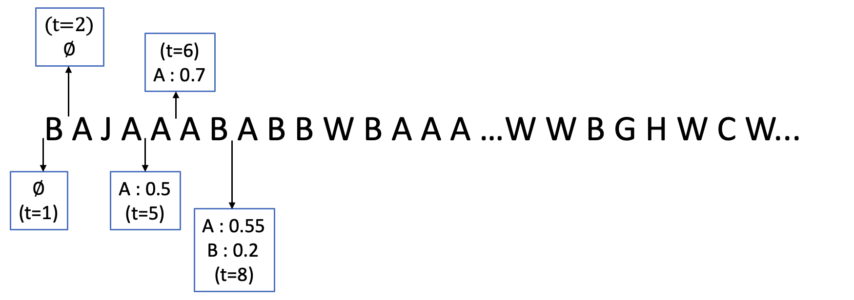
(a) An example stream of observations, left to right (items: $B$,
$A$, $J$, …), and prediction outputs, the boxes, by a hypothetical predictor
at a few of the time points shown.

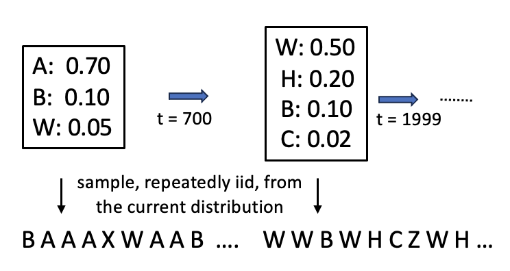
(b) A categorical distribution generates the (synthetic) data stream, in an idealized setting (iid draws), but also itself changes every so often (here, at time $t=700$, $1999$, etc).

Figure 1: (a) An example sequence of items (the capital letters) together with several prediction outputs of a hypothetical predictor, in rectangular boxes, shown for a few time points (not all outputs are shown to avoid clutter). The sequence is observed from left to right, thus at time $t=1$, item $B$ is observed ($o^{(1)}=$ $B$), and respectively at times $2$, $3$, and $4$, items $A$, $J$, and again $A$ are observed ($o^{(3)}=$ $J$, $o^{(4)}=$ $A$, etc). A prediction output is a map of item to probability (PR), and can be empty. Mathematically, it is a semi-distribution SD (Sect. 2.1). At each time point, before the observation, the predictor predicts, i.e. provides a SD (zero or more items, each with a PR). In this example, at times $t\leq 4$, nothing is predicted (empty maps, or $Q^{(1)}=Q^{(4)}=\{\}$, and only two empty outputs, at $t=1$ and $t=2$, are shown). At $t=8$, $Q^{(8)}$ is predicted, where $Q^{(8)}=\{$$A$:0.55, $B$:0.2$\}$ (i.e. $A$ is predicted with PR 0.55, and $B$ with PR 0.2). (b) The input sequence can be imagined as being generated by a SD $\mathcal{P}$: at each time point, for the next entry of the sequence, an item is drawn, iid (Sect. 2.1.1). However, the SD $\mathcal{P}$ changes from time to time, such as certain item(s) being removed and new item(s) inserted in $\mathcal{P}$. In the above example, in changing from the left (initial) $\mathcal{P}^{(1)}$ to the right distribution, $\mathcal{P}^{(2)}$ (at $t=700$), $A$ is dropped (becomes 0 PR), while $H$ and $C$ are inserted, and $W$ increases in PR while $B$ is unchanged.

Our setting is online multiclass probabilistic prediction. Time is discrete and is denoted by the variable $t$, $t=1,2,3,\cdots$. A predictor processes a stream of items (observations): at each time, it predicts then observes. Exactly one (discrete) item occurs and is observed at each time $t$ in the stream. The item or observation at time $t$ is denoted by the variable $o^{(t)}$. The parenthesized superscript notation is used for other sequenced objects as well, for instance an estimated probability $\hat{p}$ at time $t$ is denoted $\hat{p}^{(t)}$, though we may drop the superscript at times whenever the context is sufficiently clear (that it is at a particular time point is implicit). We use the words “sequence” and “stream” interchangeably, but stream is used often to imply the infinite or indefinite aspect of the task, while “sequence” is used for the finite cases, e.g. for evaluations and comparisons of prediction techniques. A sequence is denoted by the brackets, or array, notation $[\ ]$, thus $[o]_{1}^{N}$ denotes a sequence of $N$ observations: $[o^{(1)}$, $o^{(2)}$, …, $o^{(N)}]$ (also shown without commas $[o^{(1)}o^{(2)}\cdots o^{(N)}]$). We use letters $A$, $B$, $C$, $\cdots$ and also integers $0,1,2,3,\cdots$ for referring to specific items in examples. Fig. 1(a) shows an example sequence. Online processing, of an (infinite) stream or a (finite) sequence, means repeating the predict-observe-update cycle, Fig. 2(a): at each time point, predicting and then observing, and the predictor is an online learner that updates its data structures after each observation. Each item is represented and identified by an integer or string id in the various data structures (sequences, maps, …). Table 1 provides a summary of the main notations and terminology used in this paper. Sect. 3.7 describes the format we use for pseudocode, when we have presented pseudocode for a few functions.

2.1 Probabilities (PRs), Distributions (DIs), and Semi-distributions (SDs)

We use the abbreviation PR to refer to a probability, i.e. a real number in $[0,1]$. Prediction is probabilistic, and in particular in terms of semi-distributions: A semi-distribution (SD) $Q$, in this paper, is a real-valued (or PR-valued) function defined over a finite or infinite set of items $\mathcal{I}=\{0,1,2,\cdots\}$, such that $\forall i,Q(i)\in[0,1]$, and $\sum_{i\in\mathcal{I}}Q(i)\leq 1.0$. Whether or not $\mathcal{I}$ is infinite, the support, denoted $\sup(Q)$, i.e. the set of items $i$ with $Q(i)>0$, is finite in the SDs that we work with. We use $\mbox{sum}(Q)$ to denote $\sum_{i\in\mathcal{I}}Q(i)$, and $\min(Q)=\min_{i\in\sup(Q(i))}Q(i)$ (and defined as 0 if the support is empty, i.e. when $\mbox{sum}(Q)=0$). When $\mbox{sum}(Q)>0$ we say $Q$ is non-empty, and when $0<\mbox{sum}(Q)<1$, we call $Q$ a strict SD. A probability distribution (DI) $\mathcal{P}$ is a special case of a SD, where $\mbox{sum}(\mathcal{P})=1$. From a geometric viewpoint, DIs are points on the surface of a unit-simplex, while SDs can reside in the inside of the simplex too: a typical predictor’s predictions SD $Q$ starts at 0 and, with many updates to it, moves towards the surface of the simplex. The prediction output at a certain time $t$ is denoted $Q^{(t)}$, and we can imagine that a prediction method is any online technique for converting a sequence of observations, $[o]_{1}^{N}$, one observation at a time, into a sequence of predictions $[Q]_{1}^{N}$ (of equal length $N$), as shown in Fig. 2(b). But note that $Q^{(t)}$ is output before observing $o^{(t)}$ (prediction occurs before observing and updating).

A SD is implemented via a map data structure: item $\rightarrow$ (positive) PR (or $\mathcal{I}\rightarrow(0,1]$), where the keys are item ids and the values are (positive) PRs. The map can be empty, i.e. no predictions (for instance, initially at $t=1$). We use $\mathcal{P}$ to refer to an underlying or actual SD generating the observations, in the ideal setting (see next), and $Q$ to refer to estimates and prediction outputs (often strict SDs).

We use braces and colons for presenting example SDs (as in the Python programming language). For instance, with $\mathcal{P}=\{0$:0.5, 1:$0.2\}$, $\mathcal{P}$ has support size of 2, corresponding to a binary event (a coin toss), and item $0$ has PR 0.5, and $1$ has probability $0.2$, $min(\mathcal{P})=0.2$, and $\mbox{sum}(\mathcal{P})=0.7$, so $\mathcal{P}$ is a strict SD in this example.

2.1.1 Generating Sequences: an Idealized Stream

We develop prediction algorithms with the idealized non-stationary setting in mind, which we describe next. Of course, real-world sequences can deviate from this idealization in numerous ways, motivating empirical comparisons of the techniques developed on real-world datasets.

Under the stationary iid assumption or generation setting, an idealized setting, we imagine the sequence of observations being generated via independently and identically drawing (iid) items, at each time point, from a true (actual or underlying) SD $\mathcal{P}$. Because $sum(\mathcal{P})$ can be less than 1, not exhaustively covering the probability space, we explain what it means to generate from a SD below. Under an idealized but non-stationary setting, we assume the sequence of observations is the concatenation of subsequences of different lengths, where each subsequence follows the stationarity setting, and is long enough for (approximately) learning the PRs. Thus one can imagine a sequence of SDs $[\mathcal{P}]=\mathcal{P}^{(1)},\mathcal{P}^{(2)},\cdots$ (Fig. 1(b)), and the $j$th subsequence of observations, $[o]_{t_{j}}^{t_{j+1}}$, is generated by $\mathcal{P}^{(j)}$, for some duration $t_{j+1}-t_{j}$. Thus each subsequence corresponds to a stable period or phase, stationary iid setting, where the underlying SD $\mathcal{P}$ is not changing. We assume that each subsequence, corresponding to a stable period, is long enough for learning the new PRs: any item with a new PR should be observed sufficiently many times, before its PR changes in a subsequent SD $\mathcal{P}$. In synthetic experiments (Sect. 7.2 and 7.3), we define an observation-count threshold $O_{min}$ as a way of controlling the degree of non-stationarity, and we report the prediction performance of various predictors in a few such settings.

2.1.2 Salient and Noise (NS) Items, and Generating with Noise

In this paper, we are interested in predicting and evaluating PRs $p$ that are sufficiently large, $p\geq P_{min}$, where $P_{min}=0.01$ in most experiments. With respect to a SD $Q$, an item $i$ is said to be salient iff $Q(i)\geq P_{min}$, and otherwise it is NS (non-salient, or noise, or not seen recently sufficiently often). If $Q$ is the output of a predictor, we say the predictor (currently) regards $i$ as salient or NS as appropriate. In synthetic experiments, when the underlying SD $\mathcal{P}$ is known, an item is either truly salient or NS, and as $\mathcal{P}$ is changed, the same item $i$ may be NS at one point ($\mathcal{P}^{(t)}(i)<P_{min}$), and become salient at another ($\mathcal{P}^{(t+1)}(i)\geq P_{min}$), and change status several times. In practice, in evaluations, when we do not have access to a true $\mathcal{P}$, we use a simple NS marker based on whether an item has occurred sufficiently often (see 3.6). A challenge for any predictor is to quickly learn to predict new salient items while ignoring the noise.

For sequence generation, when drawing from a SD $\mathcal{P}$, with probability $1-sum(\mathcal{P})$ we generate a noise (NS) item. A simple option that we use in most experiments is to generate a unique noise id: the item will appear only once in the sequence. Sect. 7.3 explains how we generate sequences with NS items in the synthetic experiments (see also 3.9). For evaluation too, NS items need to be handled carefully, specially when using log-loss. See Sect. 3.6.

2.1.3 Binary Sequences, and the Stationary Binary Setting

The stationary binary setting, and binary sequences generated in such settings, will be useful in the empirical and theoretical analyses of the prediction techniques we develop. A stationary binary sequence is generated via iid drawing from a DI $\mathcal{P}=\{$ 1$:{p^{*}}$, 0$:1-{p^{*}}\}$, where ${p^{*}}>0$ is the true or target PR to estimate well via a predictor that processes the binary sequence. A binary sequence arises whenever we focus on a single item, say item $A$, in a given original sequence containing many (unique) items. The original sequence $[o]$ is converted to a binary $[o_{b}]$, $[o]\rightarrow[o_{b}]$, in the following manner: if $o^{(t)}=A$ then $o_{b}^{(t)}=1$, and $o_{b}^{(t)}=0$ otherwise (or $o_{b}^{(t)}=\!\left[\left[o^{(t)}=A\right]\right]$, where $\!\left[\left[x\right]\right]$ denotes the Iverson bracket on the Boolean condition $x$).

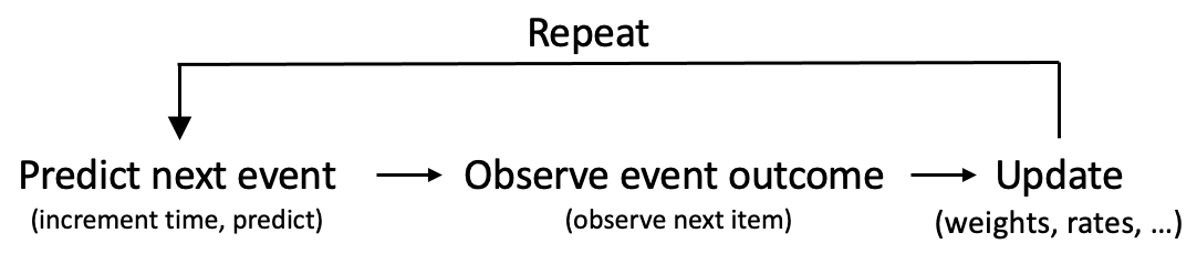
(a) Online learning: the predict-observe-update cycle.

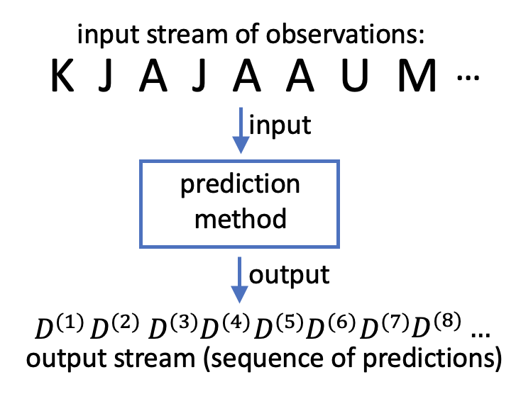
(b) A prediction method converts an item stream into a stream of SDs, the predictions.

Figure 2: (a) Online processing a stream or sequence means repeating the predict-observe-update cycle (b) A prediction method is a way of converting a stream of item observations, $[o]$, to a stream of predictions, $[Q]$, or $[o]_{1}^{N}\rightarrow[Q]_{1}^{N}$.

3 Evaluating Probabilistic Predictors

In this section we develop and discuss techniques for evaluating probabilistic multiclass sequential prediction in the face of non-stationarity. As Fig. 2(b) shows, a prediction technique is any method that converts a sequence of observations, $[o]_{1}^{N}$, into a same-length sequence, $[Q]_{1}^{N}$, of predictions, each sequence member $Q^{(t)}$ is an SD, where $Q^{(t)}$ is output before $o^{(t)}$ is observed. We develop methods for evaluating the predictions $[Q]_{1}^{N}$, given $[o]_{1}^{N}$, and possibly other extra information. A minimal desirable would be that in the stationary iid setting, when there is a true non-changing model (a distribution) that is generating the data, that a predictor quickly converges in its predictions to a good approximation of the true model. We develop this further here.

3.1 Deviation Rates: when True PRs are Known

For the purposes of evaluating the estimated PRs, we first assume we know the true PRs, which is the case in our synthetic experiments. In particular, we begin with the binary iid setting of Sect. 2.1.3 where we have a generated binary sequence with ${p^{*}}$ being the PR of 1. We take a prediction method and feed it this sequence: it processes this sequence and generates a sequence of probability estimates. Let $[\hat{p}]_{1}^{N}$ denote its sequence of estimates for the positive, 1, outcome. Thus $\hat{p}^{(t)}$ is the estimated PR at time $t$, $\hat{p}^{(t)}\geq 0$. Here, we motivate performance or error measures (quality of output probabilities) that are based on relative error or ratio, a function of $\frac{\hat{p}^{(t)}}{{p^{*}}}$, vs. based on the difference in magnitude ${p^{*}}-\hat{p}^{(t)}$ (such as the quadratic $({p^{*}}-\hat{p}^{(t)})^{2}$).

In many applications, including the prediction games setting, different items carry different rewards, and the system needs to select a subset of items to optimize an expected utility measure (expected reward). Sufficient accuracy of the PRs that the different items receive is important. While we do not specify the rewards in this paper, nor the particular way the expected reward is computed, in general, we seek to limit the relative error in estimating probabilities. For instance, as we are computing expectations, confusing a one-in-twenty event (true PR or target probability ${p^{*}}=0.05$) with a one-in-one-hundred event (${p^{*}}=0.01$), could be considered a worse error, compared to predicting an event with ${p^{*}}=0.55$ with an estimated PR of $0.5$ (even though the absolute difference in the latter two is higher).

In particular, with the true probability ${p^{*}}$, ${p^{*}}>0$, and the estimates $\hat{p}^{(t)}$ forming a sequence $[\hat{p}]_{1}^{N}$, for a choice of a deviation bound $d$, eg $d=2$, we define the deviation-rate $dev([\hat{p}]_{1}^{N},{p^{*}},d)$ as the following sequence average:

$$dev([\hat{p}]_{1}^{N},{p^{*}},d)=\frac{1}{N}\sum_{t=1}^{N}deviates(\hat{p}^{(t)},{p^{*}},d)\hskip 15.17719pt\mbox{(the deviation rate, with ${p^{*}}>0$)}$$ (1)

$$deviates(\hat{p},{p^{*}},d)=\!\left[\left[\hat{p}=0\mbox{, or (otherwise), }\max(\frac{{p^{*}}}{\hat{p}},\frac{\hat{p}}{{p^{*}}})>d\right]\right]\hskip 15.17719pt\mbox{(the deviates() value is 0 or 1)}$$ (2)

where $\!\left[\left[x\right]\right]$ is the Iverson bracket, yielding value 1 when condition $x$ is true, and 0 otherwise. Note that when $\hat{p}$ is 0, the condition is true and $deviates(0,{p^{*}},d)$ is 1 for any $d$. We seek a small deviation-rate, i.e. a large deviation, when $\max(\frac{{p^{*}}}{\hat{p}^{(t)}},\frac{\hat{p}^{(t)}}{{p^{*}}})>d$, occurs on a sufficiently small fraction of times $t$ only, e.g. say 10% of the time or less. While initially, the first few times a predictor observes an item, we may get large deviations, we seek methods that reach lowest possible deviation-rates as fast as possible. We do not specify what $d$ should be, nor what an acceptable deviation rate would be (which depends on the sequence, i.e. what is feasible, in addition to the prediction method), but, in our synthetic experiments (Sect. 7), where we know the true PRs, we report deviation rates for a few choices of $d$. More generally, we track multiple item PRs, and we will report two variations: at any time $t$, when the observed item’s estimated PR deviates, and when any (salient) item in $\mathcal{P}$ suffers too large of a deviation (Sect. 7.3).

Deviation rates are interpretable, but often in real-world settings, we do not have access to true PRs. Therefore, we also report on logarithmic loss (log-loss), and this approach is discussed and developed next, in particular for the case of SDs and NS items.

3.2 Unknown True PRs: Proper Scoring

Data streams from a real world application are often the result of the confluence of multiple interacting and changing (external) complex processes. But even if we assume there is a (stationary) DI $\mathcal{P}$ that is sampled iid, and thus true PRs exist, remaining valid for some period of time, see Sect. 2.1.1), most often, we do not have access to $\mathcal{P}$. This is a major challenge to evaluating probabilistic predictions. There exist much work and considerable published research literature, in diverse domains such as meteorology and finance, addressing the issues of unknown underlying PRs, when predicting with (estimated) PRs. In particular, the concept of proper scoring rules has been developed to encourage reliable probability forecasts [6, 17, 45, 49, 16, 46]. A proper scoring rule would lead to the best possible score (lowest if defined as costs, as we do here) if the technique’s PR outputs matched the true PRs. Not all scoring rules are proper, for instance, plain absolute loss (and linear scoring) is not proper [6]. And some are strictly proper, i.e. the true DI is the unique minimizer of the score [16]. Two major families of proper scoring rules are either based on (simple functions of) the predicted PRs raised to a power, a quadratic variant is named after Brier [6], or based on the logarithm (log probability ratios) [17, 45]: log-loss and variants. Propriety may not be sufficient, and a scoring rule also implicitly imposes measures of closeness or (statistical) distance on the space of candidate SDs, and we may prefer one score over another based on their differences in sensitivity.

We review proper scoring and the two major proper scorers below, log-loss and quadratic loss, specializing their distance property for our more general setting of SDs in particular, and we argue below, that in our utility-based or reward-based application, we strongly favor log-loss over quadratic scoring, for its better support for PRs with different scales and decision theoretic use of the estimations, and despite several desirable properties of the quadratic (such as boundedness and symmetry) in contrast to log-loss, and that we have to do extra work to adapt log-loss for handling 0 PRs (NS items). See also [12, 36] for other considerations in favor of log-loss .

3.3 Scoring Semi-Distributions (SDs)

For scoring (evaluating) a candidate distribution, we assume there exists the actual or true, but unknown, distribution (DI) $\mathcal{P}$. We are given a candidate SD $Q$  (e.g. , the output of a predictor), as well as $N$ data points, or a sequence of $N$ observations $[o]_{1}^{N}$, $t=1,\cdots,N$, to (empirically) score the candidate. Recall that we always assume that the support set of a SD is finite, and here we can assume the set $\mathcal{I}$ over which $\mathcal{P}$ and $Q$ are defined is finite too, e.g. the union of the supports of both. It is possible that the supports are different, i.e. there is some item $j$ that $Q(j)>0$, but $\mathcal{P}(j)=0$, and vice versa.

A major point of scoring is to assess which of several SD candidates is best, i.e. closest to the true $\mathcal{P}$ in some (acceptable) sense, even though we do not have access to the DI $\mathcal{P}$. It is assumed that for the time period of interest, the true generating DI $\mathcal{P}$ is not changing, and the data points are drawn iid from it. The score of a SD $Q$ is an expectation, and different scorers define the real-valued function $\mbox{ScoringRule}(Q,o)$ (i.e. the “scoring rule”) differently:

$$\mbox{Loss}(Q|\mathcal{P})={\mathbb{E}_{o\sim\mathcal{P}}}(\mbox{ScoringRule}(Q,o))\hskip 36.135pt\mbox{(the loss or score of a SD $Q$, given true DI $\mathcal{P}$)}$$ (3)

Thus the Loss() (score) of a SD $Q$ is the expected value of the function ScoringRule(), where the expectation is taken with respect to (wrt) the true DI $\mathcal{P}$. In practice, we compute the average AvgLoss()  as an empirical estimate of Loss:

$$\mbox{AvgLoss}(Q)=\frac{1}{N}\sum_{t=1}^{N}\mbox{ScoringRule}(Q,o^{(t)})\hskip 36.135pt\mbox{(the average: an empirical estimate of the loss)}$$ (4)

computed on the $N$ data points (assumed drawn iid using $\mathcal{P}$). Thus, for scoring a candidate SD $Q$, i.e. computing its (average) score, we do not need to know the true DI $\mathcal{P}$, but only need a sufficiently large sample of $N$ points drawn iid from it. However, for understanding the properties of a scoring rule, the actual SD  $\mathcal{P}$ is important. In particular, as further touched on below, the score is really a function of an (implicit) statistical distance between the true and candidate distributions. The details of the scoring rule definition, ScoringRule(), determines this distance. Different scoring functions differ on the scoring rule $\mbox{ScoringRule}(Q,o)$, i.e. how the PR outputs of SD, given the observed item was $o$, is scored. We also note that the minimum possible score, when $Q=\mathcal{P}$ (for strictly proper losses), can be nonzero. We next define the QuadLoss (Brier) scoring rule and loss.

3.4 The Quadratic (Brier) Score, and its Insensitivity to PR Ratios

The Quadratic score of a candidate SD, QuadLoss, is defined as:

$$\mbox{QuadLoss}(Q|\mathcal{P}):={\mathbb{E}_{o\sim\mathcal{P}}}(\mbox{QuadRule}(Q,o)),\mbox{ where \ }\mbox{QuadRule}(Q,o):=\sum_{i\in\mathcal{I}}(\delta_{i,o}-Q(i))^{2},$$ (5)

where $\delta_{i,o}$ denotes the Kronecker delta, i.e. $\delta_{i,o}=1$ when $o=i$ and 0 otherwise ($\delta_{i,o}=0$ for $i\neq o$) and an equivalent expression is $\mbox{QuadRule}(Q,o)=(1-Q(o))^{2}+\sum_{i\in\mathcal{I},i\neq o}Q(i)^{2}$. Note that at each time point $t$, to compute the value of QuadRule()  (the loss or cost over an observation), we go over all the items in $\mathcal{I}$, and we have $0\leq\mbox{QuadRule}(Q,o)\leq 2.0$. One can view the scoring rule QuadRule() as taking the (squared) Euclidean distance between two vectors: the Kronecker vector, i.e. the vector with Kronecker delta entries (all 0, except the dimension corresponding to observed item $o$), and the probability vector corresponding to the SD $Q$.

Compared to the log-loss of the next section, the Brier score can be easier to work with, as there is no possibility of “explosion”, i.e. unbounded values (see Sect. 3.5). However, in our application we are interested in probabilities that can widely vary, for instance, spanning two orders of magnitude ($\mathcal{P}(i)\geq 0.1$ for some $i$, and $\mathcal{P}(j)$ near $0.01$ for other items), and as mentioned above, different items are associated with different rewards and we are interested in optimizing expected rewards. Thus confusing a one-in-twenty event with a substantially lower probability event, such as a zero probability event, can incur considerable underperformance (depending on the rewards associated with the items).

In particular, for instance in [42], QuadLoss), when both $\mathcal{P}$ and $Q$ are DIs, it is established that the QuadLoss score is equivalent to (squared) Euclidean distance to the true probability distribution, where the distance is defined as:

$$\mbox{QuadDist}(Q_{1},Q_{2}):=\sum_{i\in\mathcal{I}}(Q_{1}(i)-Q_{2}(i))^{2}\mbox{\ \ \ \ \ \ \ (defined for SDs $Q_{1}$ and $Q_{2}$)}$$

The equivalence is in the following strong sense:

Lemma 1.

(sensitivity of QuadLoss to the magnitude of PR shifts only) Given DI $\mathcal{P}$ and SD $Q$, defined over the same finite set $\mathcal{I}$,

            $\mbox{QuadLoss}(Q|\mathcal{P})=\mbox{QuadDist}(Q,\mathcal{P})$

This property has been established when both are DIs (i.e. when $\mbox{sum}(Q)=1$) [42], and similarly can be established by writing the expectation expressions, rearranging terms, and simplifying (proof provided in the Appendix A.1). Examining the distance version of the loss, we can first note that QuadLoss has a desired property of symmetry when $Q$ is also a DI, i.e. $\mbox{QuadLoss}(Q_{1}|Q_{2})=\mbox{QuadLoss}(Q_{2}|Q_{1})$ (for two DIs $Q_{1}$ and $Q_{2}$). We can also observe that QuadLoss is only sensitive to the magnitude of shifts in PRs, with $\Delta_{i}:=\mathcal{P}(i)-Q(i)$, then $\mbox{QuadLoss}(Q|\mathcal{P})=\sum_{i\in\mathcal{I}}\Delta_{i}^{2}$ (Corollary 2). It is not sensitive to source (or destination) of the original probabilities of items those quantities are transferred from: it does not particularly matter if a positive PR is reduced to 0 in going from $\mathcal{P}$ to $Q$. For instance, assume $\mathcal{P}=\{1$:$0.9$, $2$:$0.1\}$. Consider the two candidate SDs $Q_{1}=\{1$:$0.8$, $2$:$0.1\}$, $Q_{2}=\{1$:$0.9$, $2$:$0.0\}$. In terms of violating a deviation threshold (Sect. 3), $Q_{2}$ violates all ratio thresholds on item 2, and the log-loss below is rendered infinite on it, while SD $Q_{1}$ has a relatively small violation. However, for both cases $\Delta=0.1$, and we have $\mbox{QuadLoss}(Q_{1}|\mathcal{P})=\mbox{QuadLoss}(Q_{2}|\mathcal{P})=0.1^{2}$, and $Q_{1}$ and $Q_{2}$ would have similar empirical losses using the QuadLoss score.

The utility of a loss depends on the application, of course. For instance, for clustering DIs, symmetry can be important, and thus quadratic loss may be preferrable over log-loss. In our prior work, in an application where events were binary, and PRs were concentrated near 0.5 (two-team professional sports game outcomes), and where there was no single true DI but likely many, quadratic loss was adequate [9].

3.5 On the Sensitivity of log-loss

The LogLoss and the log rule are based on simply taking the $\ln$, of the probability estimated for the observation $o$, [17, 45], and thus should be sensitive to relative changes in the PRs (PR ratios):

$$\mbox{LogLoss}(Q|\mathcal{P}):={\mathbb{E}_{o\sim\mathcal{P}}}(LogRule(Q,o)),\mbox{ where \ }LogRule(Q,o)=-\ln(Q(o)),$$ (6)

The scoring rule can be viewed as the well-known KL (Kulback-Leibler) divergence of $Q$ from the Kronecker vector, i.e. the distribution vector with all 0s and a 1 on the dimension corresponding to the observed item $o$. This boils down to $-\ln(Q(o))$. Recall that for QuadLoss, QuadRule was in terms of the Euclidean distance, which involved all the items (dimensions). Indeed, similar to the development in the previous section, LogLoss can be shown to correspond to the KL divergence [21, 8]:

Definition 1.

The entropy of a non-empty SD $\mathcal{P}$ is defined as:

$$\hskip 28.45274pt\mbox{Entropy}(\mathcal{P})=-\sum_{i\in\mathcal{I}}\mathcal{P}(i)\ln(\mathcal{P}(i))$$ (7)

The KL divergence of $Q$ from $\mathcal{P}$ (asymmetric), also known as the relative entropy, denoted $\mbox{KL}(\mathcal{P}||Q)$, is a functional, defined here for non-empty SD $\mathcal{P}$ and SD $Q$:

$$\hskip 28.45274pt\mbox{KL}(\mathcal{P}||Q):=\sum_{i\in\mathcal{I}}\mathcal{P}(i)\ln\frac{\mathcal{P}(i)}{Q(i)}.$$ (8)

Note that in both definitions, by convention [8], when $\mathcal{P}(i)=0$, we take the product $\mathcal{P}(i)\ln(x)$ to be 0 (or $i$ need only go over $\sup(\mathcal{P})$, in the above definitions). The divergence $\mbox{KL}(\mathcal{P}||Q)$ can also be infinite (denoted $+\infty$) when $\mathcal{P}(i)>0$ and $Q(i)=0$.

Lemma 2.

Given DI $\mathcal{P}$ and SD $Q$, defined over the same finite set $\mathcal{I}$,

$$\hskip 28.45274pt\mbox{LogLoss}(Q|\mathcal{P})=\mbox{Entropy}(\mathcal{P})+\mbox{KL}(\mathcal{P}||Q).$$

This is established when both are DIs, for example [42], but the the derivation does not change when $Q$ is a SD: $\mbox{LogLoss}(Q|\mathcal{P})=-\sum_{i\in\sup(\mathcal{P})}\mathcal{P}(i)\ln(Q(i))=-\sum_{i\in\sup(\mathcal{P})}\mathcal{P}(i)\ln(Q(i))-\mbox{Entropy}(\mathcal{P})+\mbox{Entropy}(\mathcal{P})$ (i.e. add and subtract $\mbox{Entropy}(\mathcal{P})$), and noting that the first two terms is a rewriting of the KL(), establishes the lemma.

Note that the entropy term in log-loss is a fixed positive offset: only KL() changes when we try different candidate SDs with the same underlying $\mathcal{P}$. Again, as in Sect. 3.4, this connection to distance helps us see several properties of LogLoss. From the properties of KL [8], it follows that LogLoss is strictly proper (and asymmetric, unlike QuadLoss). Furthermore, the expression for KL divergence helps us see that log-loss is indeed sensitive to the ratios (of true to candidate probabilities). In particular, log-loss can grow without limit or simply explode (i.e. become infinite) when $\mathcal{P}(i)>0$ and $Q(i)=0$, for instance, in our sequential prediction task, when an item has not been seen before. We discuss handling such cases in the next section. On the other hand, we note that the dependence on the ratio is dampened with a $\ln()$ and weighted by the magnitude of the true PRs, as we take an expectation. In particular, we have the following property, a corollary of the connection to KL(), which quantifies and highlights the extent of this ratio dependence:

Corollary 1.

(LogLoss is much more sensitive to relative changes in larger PRs) Let $\mathcal{P}$ be a DI over two or more items (dimensions), with $\mathcal{P}(1)>\mathcal{P}(2)>0$, and let $m=\frac{\mathcal{P}(1)}{\mathcal{P}(2)}$ (thus $m>1$). Consider two SDs $Q_{1}$ and $Q_{2}$, with $Q_{1}$ differing with $\mathcal{P}$ on item 1 only, in particular $\mathcal{P}(1)>Q_{1}(1)>0$, and let $m_{1}=\frac{\mathcal{P}(1)}{Q_{1}(1)}$ (thus, $m_{1}>1$). Similarly, assume $Q_{2}$ differs with $\mathcal{P}$ on item 2 only, and that $\mathcal{P}(2)>Q_{2}(2)>0$, and let $m_{2}=\frac{\mathcal{P}(2)}{Q_{2}(2)}$. We have $\mbox{LogLoss}(Q_{2}|\mathcal{P})<\mbox{LogLoss}(Q_{1}|\mathcal{P})$ for any $m_{2}<m_{1}^{m}$.

The proof is simple and goes by subtracting the losses, $\mbox{LogLoss}(Q_{1}|\mathcal{P})-\mbox{LogLoss}(Q_{2}|\mathcal{P})$, and using the KL() expressions for the log-loss terms and simplifying (Appendix A). Thus, with a reasonably large multiple $m$, $m_{2}$ needs to be very large for $\mbox{LogLoss}(Q_{2}|\mathcal{P})$ to surpass $\mbox{LogLoss}(Q_{1}|\mathcal{P})$. As an example, let DI $\mathcal{P}=\{$1:0.5, 2:0.05, 3:0.45$\}$, then $m=10$, and reduction by $m_{1}\geq 1$, only in PR of item 1, yields LogLoss $l_{1}$ that is $\frac{m_{1}^{10}}{m_{2}}$ higher than LogLoss $l_{2}$ that would result from reducing PR of item 2 only, by $m_{2}$. For example, with $Q_{1}=\{$1:0.25, 2:0.05, 3:0.45$\}$, and with $Q_{2}=\{$1:0.5, 2:$p$, 3:0.45$\}$, as long as $p>\frac{0.05}{2^{10}}\approx 10^{-4}$, $\mbox{LogLoss}(Q_{1}|\mathcal{P})>\mbox{LogLoss}(Q_{2}|\mathcal{P})$ (or we have to reduce 0.05 a thousand times, $2^{10}$, to match the impact of just halving 0.5 to 0.25).

When we report deviation-rates in synthetic experiments (Eq. 1), we ignore the magnitude of the PRs involved (as long as greater than $P_{min}$), but log-loss incorporates and is substantially sensitive to such. Because items with larger PRs are seen in the stream more often, such a dependence is warranted, specially when we use the PRs to optimize expected rewards (different predictands having different rewards). However, when a predictor has to support predictands with highly different PRs (e.g. at $0.5$ and $0.05$), we should anticipate that LogLoss scores will be substantially more sensitive to better estimating the higher PRs.

3.6 Developing log-loss for NS (Noise) Items

FC($Q$) // Filter & cap, given item to PR map $Q$.

// Parameters: $P_{NS},P_{min}$, both in $[0,1)$

$filtered\leftarrow$ ScaleDrop($Q$, 1.0, $P_{min}$)

If $sum(filtered)\leq 1.0-P_{NS}$: // Already capped?

Return $filtered$ // Nothing left to do.

$\alpha\leftarrow\frac{1-P_{NS}}{sum(filtered)}$ // Scale down by $\alpha$.

Return ScaleDrop($filtered$, $\alpha$, $P_{min}$)

ScaleDrop($Q$, $\alpha$, $P_{min}$) // Filter and scale $Q$ (a map).

$scaled\leftarrow\{\}$

For item $i$, PR $prob$ in $Q$:

$prob\leftarrow\alpha*prob$

If $prob\geq P_{min}:$   // Keep only the salient.

$scaled[i]\leftarrow prob$

Return $scaled$

(a) Filtering & capping a map, yielding a constrained

SD: no small PRs and the sum is capped.

loglossRuleNS($o,Q,markedNS$)

// Parameters: $P_{NS},P_{min}$. The current observation is $o$,

// and SD $Q$ is the predictions (a PR map).

$Q\leftarrow{\bf FC}(Q)$ // cap and filter.

$prob\leftarrow Q$.get$(o,0.0)$

If $prob\geq P_{min}$: // $o\in Q$?

Return $-\ln(prob)$ // plain log-loss.

// $o\not\in Q$: the predictor thinks $o$ is a new/noise item.

If not $markedNS$: // The NS-marker disagrees.

Return $-\ln(P_{NS})$ // Return the highest loss.

// The NS-marker and predictor agree $o$ is NS

// Use the unused probability mass in SD $Q$.

$p_{noise}\leftarrow 1.0-sum(Q)$ // note: $p_{noise}\geq P_{NS}$

Return $-log(p_{noise})$

(b) When computing log-loss, handling new or noise items.

Figure 3: Functions used in evaluating the probabilities. (a) CapAndFilter() is applied to the output of any prediction method, at every time point, before evaluation. It performs filtering (dropping small probabilities, below $P_{min}$) and, if necessary, explicit capping, i.e. normalizing or scaling down, meaning that the final output will be a SD $Q$, where $sum(Q)\leq 1-P_{NS}$. $P_{NS}=P_{min}=0.01$ in experiments. (b) Scoring based on log-loss and handling NS items.

In our application, every so often a predictor observes new items that it should learn to predict well. For such an item $o$, $\mathcal{P}(o)$ was 0 before some time $t$, and $\mathcal{P}(o)\geq P_{min}$ after. Some proportion of the input stream will also consist of infrequent items, i.e. truly NS (noise) items, those whose frequency, within a reasonable recent time window, falls below $P_{min}$. A challenge for any predictor is to quickly learn to predict new salient items while ignoring the noise. Plain log-loss is infinite when the predictor assigns a zero PR to an observation $o$ ($Q(o)=0$), and more generally, large losses on infrequent items can dominate overall log-loss rendering comparing predictors using log-loss uninformative and useless. We need more care in handling such cases, if log-loss is to be useful for evaluation.

Our evaluation solution has 3 components:

1. Ensuring that the output map of any predictor, whenever used for evaluation, is a SD $Q$ such that $\mbox{sum}(Q)\leq 1-P_{NS}$, with $P_{NS}>0$, thus some PR $\geq P_{NS}$, is left for possibly observing an NS item (FC() in Fig. 3(a)).

2. Using a simple NS-marker algorithm, a (3rd-party) “referee", for determining NS status, as in Fig. 4(a).

3. A scoring rule (policy) specifying how to score in the various cases, e.g. whether or not an item is marked NS (the function loglossRuleNS() in Fig. 3(b)).

Fig. 3(a) shows the pseudocode for filtering and capping, FC(), applied to the output of any prediction method, before we evaluate its output. The only requirement on the input map $Q$ passed to FC() is that the map values be non-negative. In this paper, all prediction methods output PR maps, i.e. with values in $[0,1]$, though their sum can exceed 1.0. The function removes small values and ensures that the sum of the entries is no more than $1.0-P_{NS}$, where $P_{NS}=0.01$ in our experiments. Thus the output of FC(), a map, corresponds to a SD $Q$ such that $\mbox{sum}(Q)\leq 1-P_{NS}$ and $\min(Q)\geq P_{min}$.

isNS($o$) // Return whether observation $o$ is NS or not.

// Parameters: $c_{NS}$ (NS count threshold).

// whether or not $o$ should be treated as NS .

$flagNS\leftarrow recentFrqMap.get(o,0)\leq c_{NS}$

UpdateCount($o,recentFrqMap$) // Increment count of $o$.

Return $flagNS$

(a) Pseudo code for a simple NS-marker.

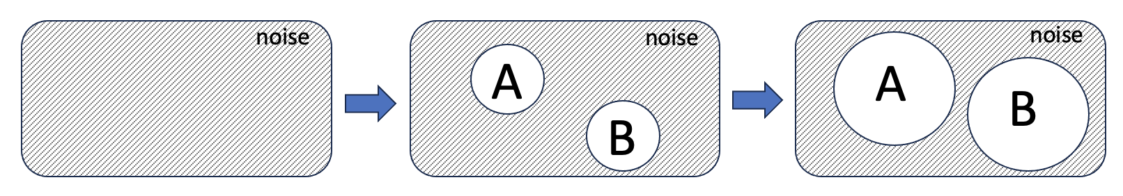
(a)

(b) Venn diagram examples, depicting background noise and underlying SD $\mathcal{P}$, here two salient items $A$ and $B$ growing in PRs as we go from left to right (middle $\mathcal{P}^{(2)}$ could be $\{$$A$:$0.1,$$B$:$0.1\}$), when plotting the lowest achievable loss in Fig. 4(c).

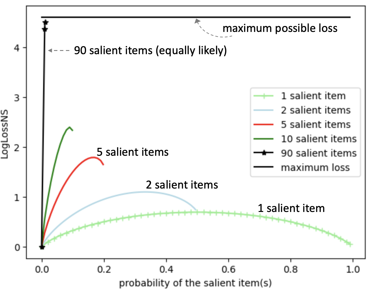
(b)

(c) Lowest achievable log-loss, via the

LogLossNS() function, under a few generation

regimes where salient item are equally likely.

Figure 4: (a) A simple NS-marker, a referee to mark an item NS or not, using a count map. (b) Venn diagrams, with background noise, are useful in picturing how sequences are generated, e.g. in synthetic experiments. Here, as we go from left to right in generating a lowest achievable loss plot of Fig. 4(c), three Venn digrams of the underlying SDs are shown for the case of two salient items (left $\mathcal{P}^{(1)}=\{\}$ while right $\mathcal{P}^{(3)}$ could be $\{$$A$:$0.25,$$B$:$0.25\}$). (c) Optimal (lowest achievable) log-loss using the LogLossNS() function of Fig. 3, as the PR of $k$ salient items, all equally likely, is increased to maximum possible ($1/k$), from left to right. The lowest loss is (near) 0 when any observed item is noise (on the left) or, on the right, when there is a single salient item with PR 1.0. Maximum loss never exceeds $-\ln(P_{min})$ ($\approx 4.6$ in this paper, with $P_{min}=0.01$) and is reached when there are $k\approx\frac{1}{P_{min}}$ salient items, each with max PR $\approx P_{min}$.

3.7 Notes on Pseudocode

We briefly describe how we present pseudocode, such as the examples of Fig. 3 and 4(b). The format is very similar to Python, e.g. using indentation to delimit a block such as function or loop body, and how we show iteration over the key and value pairs of a map. Function names are boldfaced. Importantly, not all parameters, such as flags, or state variables of a function, is given in its declaration to avoid clutter, but in the comments below its declaration, we explain the various variables used. In some cases, it is useful to think of a function as a method for an object, in object-oriented programming, with its state variables (or fields), some represented by data structures such as array or maps. For a map $Q$, $Q[i]$ is its value for key (item) $i$, but we also use $Q$.get($i,0$) if we want to specify returning 0 when key $i$ does not exist in the map. $\{\}$ denotes an empty map and $\mbox{sum}(Q)$ is the sum of its values (0 if empty map). We use $\leftarrow$ for assignment, and ’//’ to begin the comment lines (like C++). We favored simplicity and brevity at the cost of some loss in efficency (e.g. some loops may be partially redundant). Not all the functions or the details are given (e.g. in the NS-marker of Fig. 4), but hopefully enough of such is presented to clarify how each function can work.

3.8 Empirical log-loss for NS (Noise) Items

Once we have an NS-marker and the FC() function, given any observation $o^{(t)}$, and the predictions $Q^{(t)}$ (where we have applied FC() to get the SD $Q^{(t)}$) and given the NS status of $o^{(t)}$ (via the NS-marker), we evaluate $Q^{(t)}$ using loglossRuleNS(), and take the average over the sequence:

$$\mbox{AvgLogLossNS}([o]_{1}^{N},[Q]_{1}^{N})=\frac{1}{N}\sum_{t=1}^{N}\mbox{{\bf loglossRuleNS}}(o^{(t)},Q^{(t)},\mbox{{\bf isNS}}(o^{(t)}))$$ (9)

The scoring rule loglossRuleNS($o,Q,\mbox{{\bf isNS}}(o)$) checks if there is a PR $p,p>0$ assigned to $o$, $p=Q(o)$. If so, we must have $p\geq P_{min}$ (from the definition of FC()), and the loss is $-\ln(p)$. Otherwise, if $o$ is also marked NS (there is agreement), the loss is $\ln(1-\mbox{sum}(Q))$. From the definition of FC(), $1-\mbox{sum}(Q)\geq P_{NS}$. Finally, if $o$ is not marked NS, the loss is $-\ln(P_{NS})$. In all cases, the maximum loss is $-\ln(P_{NS})$. Therefore, if we are interested in obtaining bounded losses then $P_{NS}$ should be set to a positive value. On the other hand, if we are interested in learning a PR in a range down to a smallest value $p>0$, then we should set $P_{min}=p$ and we should have $P_{NS}\leq P_{min}$. In our experiments, $P_{min}=P_{NS}=0.01$. By default, we set $c_{NS}=2$ for NS-marker, but we also report comparisons for other values in a few experiments to assess sensitivity of our comparisons to $c_{NS}$. When comparing different predictors, computing and comparing AvgLogLossNS() scores, we will often compare on the same exact sequences and use an identical NS-marker. We discuss a few alternative options to this manner of evaluation in the appendix, Sect. A.4.

3.9 The Near Propriety of loglossRuleNS

We first formalize drawing items using a SD $\mathcal{P}$, which enables us to define taking expectations wrt a SD $\mathcal{P}$. For this, it is helpful to define the operation of multiplying a scalar with a SD, or scaling a SD , which is also extensively used in deriving various optimality properties of candidate SDs (Appendix A.3).

Definition 2.

Definitions related to generating sequences using a SD, and perfect filtering and NS-marker wrt to a SD:

• (scaling a SD) Let SD $\mathcal{P}$ be non-empty, i.e. $\mbox{sum}(\mathcal{P})\in(0,1]$. Then, for $\alpha>0,\alpha\leq\frac{1}{\mbox{sum}(\mathcal{P})}$, $\mathcal{P}^{\prime}=\alpha\mathcal{P}$ means the SD where $\forall i\in\sup(\mathcal{P})$, $\mathcal{P}^{\prime}(i)=\alpha\mathcal{P}(i)$. When $\alpha=\frac{1}{\mbox{sum}(\mathcal{P})}$, $\alpha\mathcal{P}$ is a DI and one can repeatedly draw iid from it.

• Drawing an item from a non-empty SD $\mathcal{P}$, denoted $o\sim\mathcal{P}$, means $\mbox{sum}(\mathcal{P})$ of the time, drawing from $\alpha\mathcal{P}$, where $\alpha=\frac{1}{\mbox{sum}(\mathcal{P})}$ (SD $\mathcal{P}$ scaled up to a DI), and $1-\mbox{sum}(\mathcal{P})$ of the time generating a unique noise item. Repeatedly drawing items in this manner $N$ times to get $[o]_{1}^{N}$, "iid drawing" from $\mathcal{P}$, is denoted $[o]_{1}^{N}\sim\mathcal{P}$.

• (perfect marker) Given a non-empty SD $\mathcal{P}$, a perfect NS-marker wrt to $\mathcal{P}$, marks an item $i$ as NS iff $i\not\in\sup(\mathcal{P})$.

Therefore, for a DI $\mathcal{P}$, a perfect NS-marker generates no NS markings on a sequence $[o]_{1}^{N}\sim\mathcal{P}$.

Given a non-empty SD $\mathcal{P}$, LogLossNS(), given FC() and an NS-marker, is defined as:

$$\mbox{\bf LogLossNS}(Q|\mathcal{P}):={\mathbb{E}_{o\sim\mathcal{P}}}(\mbox{{\bf loglossRuleNS}}(o,Q,isNS(o)))$$ (10)

Thus AvgLogLossNS() is the empirical average version of LogLossNS(), where we use a practical NS-marker. We show in the Appendix that in the iid generation setting based on SD $\mathcal{P}$, and when using FC() with parameters $P_{NS}$ and $P_{min}$, $\mathcal{P}$ will score highest in several cases, and otherwise, a $Q$ scoring high is close to $\mathcal{P}$ in a certain sense, when $P_{NS}$ and $P_{min}$ are small.

3.10 Understanding the Behavior of LogLossNS

Fig. 4(c) shows the lowest achievable loss, the optimal loss, when using LogLossNS() in a few synthetic scenarios: as the PR of $k\geq 1$ equally likely salient items is raised from 0 to near $k^{-1}$ each, and where we assume an item is marked seen only when its true PR is above $P_{min}$ (and $P_{min}=P_{NS}=0.01$). On the left extreme, there are no salient items (all PRs at 0 or below $P_{min}$), and a predictor achieves 0 loss by predicting an empty map, i.e. no salient items ($\mbox{sum}(Q)=0$). Here, both the NS-marker and the predictor agree that every observed item is noise. Next, consider the case of one (salient) item as its PR is raised from $P_{min}$. At the right extreme, where its probability nears 1.0, the minimum achievable loss approaches 0 as well. Note that due to the capping, we never get 0 loss (with $P_{NS}=0.01$, we get $-\ln(0.99)\approx 0$). Midway, when ${p^{*}}$ is around 0.5, we get the maximum of the optimum curve, yielding LogLossNS around $-\ln(0.5)$ (the salient item is observed half the time, and half the time both the NS-marker and predictor agree that the item observed is noise, with $p_{noise}=0.5$). Similarly, for the scenarios with $k>1$ items, the maximum optimal loss is reached when the items are assigned their maximum allowed probability, i.e. $\frac{1}{k}$.

Fig. 4(b) shows a useful way to pictorially imagine a sd $\mathcal{P}$ that is generating the observation sequence as a Venn diagram. Salient items are against a background of noise, and when we change $\mathcal{P}$, for instance increase the PR of a salient item $A$, the area of its corresponding blob increases, and this increase can be obtained from reducing the area assigned to the background noise (as in Fig. 4(b) and the experiments of Fig. 4(c)), or one or more other salient item can shrink in area (while total area remaining constant at 1.0). When drawing, each item, including noisem, is picked with PR proportional to its area.

3.11 Nonstationarity

We can use the same empirical evaluation log-loss formula of AvgLogLossNS() (Eq. 9) in the idealized non-stationary case, and as long as each subsequence is sufficiently long, a convergent prediction method should do well. In synthetic experiments, we try different minimum frequency requirements on items, before their probability is changed, when generating sequences. In real-world sequences, a variety of phenomena such as periodicity and other dependencies can violate the iid assumption, and it is an empirical question whether the predictors compare as anticipated based on their various strengths and weaknesses. This underscores the importance of empirical experiments on different real-world sequences.

4 Sparse EMA for Probabilistic Multiclass Prediction

Our first predictor is the (sparse) exponentiated moving average (EMA), which we have used for multiclass prediction, specially suited to non-stationarity [31, 29]. Fig. 5 presents pseudo code. The predictor keeps a map, of item to PR, and it can be shown that the map is always a SD [31]. Initially, at $t=1$, the map is empty. Each map-entry can be viewed as a connection, or a prediction relation, a weighted directed edge, from the predictor to a predictand, where the weight is the current PR estimate for the predictand. Prediction is straightforward: output the map’s key-value (or key-PR) entries. An EMA update is a convex combination of the present observation with the past (running) average. When learning proportions as in this paper, the observation is either 0 or 1, and the update can be broken into two phases, first a weakening of the weights, of edges to existing predictands, which can be seen as PRs flowing from existing edges into an implicit (available) PR reservoir, and then a strengthening to the observed item, PR flowing from the reservoir to the target edge, as pictured in Fig. 6. This picture is useful when we extend EMA (Sect. 6). We next describe challenges of PR estimation, in particular speed of convergence vs. variance, and handling non-stationarity (versions of plasticity vs. stability trade-offs [1, 34]), motivating extensions of plain EMA.

EmaUpdate($o$) // latest observation $o$.

// $EmaMap$ is a map: item to PR. Learning rate $\beta\in(0,1]$,

// Other: $doHarmonicDecay$ flag.

For each item $i$ in $EmaMap$:

$EmaMap[i]\leftarrow(1-\beta)*EmaMap[i]$ // Weaken.

// Strengthen connection to $o$ (insert edge if not there).

$EmaMap[o]\leftarrow EmaMap[o]+\beta$

If $doHarmonicDecay$: // reduce rate?

$\beta\leftarrow DecayRate(\beta)$

DecayRate($\beta$)

// Other parameters: $\beta_{min}\in(0,1)$, the minimum

// allowed learning rate. $\beta_{max}\in(0,1]$, the maximum

// initial learning rate for EMA with harmonic decay.

$\beta\leftarrow\frac{1}{\frac{1}{\beta}+1.0}$ // harmonic decay.

Return $\max(\beta,\beta_{min})$

Figure 5: Pseudo code of sparse EMA with a single learning rate $\beta$, either fixed ("static" EMA), or decayed with a harmonic schedule down to a minimum $\beta_{min}$ ("harmonic" EMA). The working of an EMA update can be split in two steps (Fig. 6): 1) weaken, i.e. weaken all existing edge weights (map entries), and 2) strengthen, i.e. boost (the weight of) the edge to the observed item (target). The map entry is created if it doesn’t already exist (edge insertion). Initially (at $t=1$), there are no edges. EMA enjoys a number of desirable properties, such as the probabilities forming a SD, and approximate convergence (Sect. 4).

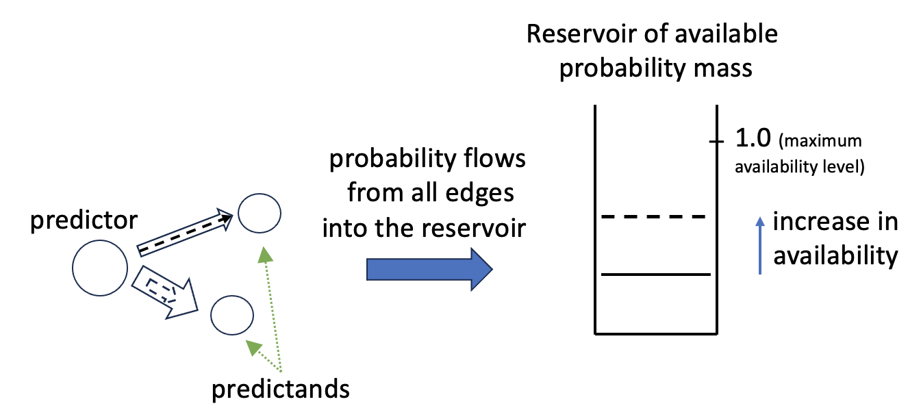
(a) First phase of EMA: weaken all edges.

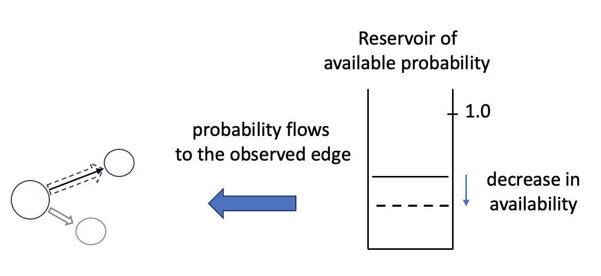
(b) Second phase: boost weight of target.

Figure 6: An EMA update can be seen as having two phases. In the first phase, all existing edges from the predictor to the predictands (entries in the map) are weakened, which can be viewed as probability flowing from the edges to the (unused) reservoir (the edges, after the weakening, reduced in weight, are shown smaller and dotted). In the 2nd phase, the edge to the observed item is strengthened. The reservoir is implicit: with SD $Q$ corresponding to the map, the reservoir has PR mass $1-\mbox{sum}(Q)$. Initially (at $t=1$), with an empty map (no edges), the reservoir is at 1.0.

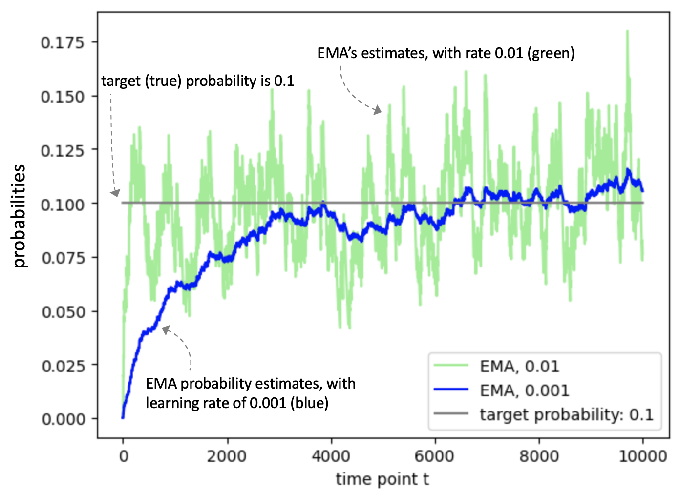
(a) EMA convergence under different (fixed) rates, $\beta=0.01$ and $\beta=0.001$ (binary iid setting). Higher rates can yield faster convergence, but also higher variance.

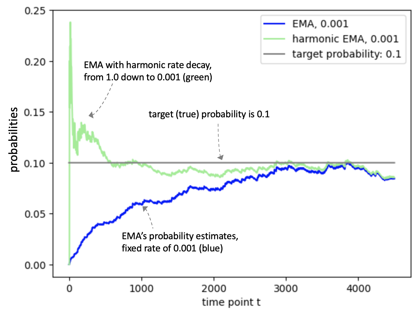
(b) Harmonic decay of rate speeds convergence for higher target PRs such as ${p^{*}}=0.1$ (vs. static EMA).

Figure 7: Given a single binary sequence, 10k long, with target ${p^{*}}=0.1$ (the true PR of observing 1), convergence of the PR estimates, $\hat{p}^{(t)}$, by EMA variants: (a) for the static or fixed-rate version of EMA, under two different learning rates, $\beta=0.01$ and $\beta=0.001$. A higher rate, $\beta=0.01$, can lead to faster convergence, but also causes high variance. (b) With harmonic decay, the estimates converge faster (possibly with a high-variance initial period).

deviation threshold $\rightarrow$	$d=1.5$		$d=2.0$
learning rate $\rightarrow$	$\beta={p^{*}}/5$	$\beta={p^{*}}/20$	$\beta={p^{*}}/5$	$\beta={p^{*}}/20$
${p^{*}}=0.1$	47, 0.19 $\pm 0.02$	213, 0.01$\pm 0.01$	35, 0.04$\pm 0.01$	140, 0.001$\pm 0.002$
${p^{*}}=0.01$	520, 0.20$\pm 0.08$	2200, 0.04$\pm 0.05$	350, 0.05$\pm 0.04$	1400, 0.02$\pm 0.03$

Table 2: 10k-long sequences, 500 trials, for two target probabilities ${p^{*}}$, ${p^{*}}=0.1$ and ${p^{*}}=0.01$, and for two $\beta$ settings for EMA, $\frac{{p^{*}}}{5}$ and $\frac{{p^{*}}}{20}$, the first time EMA’s estimate $\hat{p}^{(t)}$ reaches to within deviation threshold $d$ (averaged over the trials), and the deviation-rate thereafter (and the std over the 500 trials) are reported. The initial estimate is 0 ($\hat{p}^{(1)}=0$). For instance, when ${p^{*}}=0.1$, EMA with $\beta=\frac{{p^{*}}}{5}=0.02$ takes 47 time points on average to reach within $d=1.5$ of ${p^{*}}=0.1$ and thereafter it has deviation-rate of 19% (while with $\beta=\frac{{p^{*}}}{20}$, it has only 1% deviation-rate). A higher rate leads to faster convergence for EMA, but also higher variance.

4.1 Convergence

It can be shown that the EMA update, with $\beta\in[0,1]$, preserves the SD property: when the PR map before the update corresponds to a SD $Q^{(t)}$, $Q^{(t+1)}$ (the map after the update) is a SD too. Furthermore, EMA enjoys several convergence properties under appropriate conditions, e.g. the sum of the edge weights (map entries) increases, converging to 1.0 (i.e. to a DI), and an EMA update can be seen to be following the gradient of quadratic loss [31]. Here, we are interested in convergence of the map weights as individual PR estimates.

In the stationary iid setting (Sect. 2.1.1), we show that the PR estimates of EMA converge, probabilistically, to the vicinity of the true PRs. We focus on the EMA estimates for one item or predictand, call it $A$: at each time point $t$, a positive update occurs when $A$ is observed, and otherwise it is a negative update (a weakening), which leads to the stationary binary setting (Sect. 2.1.3), where the target PR is denoted ${p^{*}}$. The estimates of EMA for item $A$, denoted $\hat{p}^{(t)}$, form a random walk. While often, i.e. at many time points, it can be more likely that $\hat{p}^{(t)}$ moves away from ${p^{*}}$, such as when $\hat{p}\leq{p^{*}}<0.5$, when $\hat{p}$ does move closer to ${p^{*}}$ (upon a positive observation), the gap reduces by a relatively large amount. The following property, in particular, helps us show that the expected gap, $|{p^{*}}-\hat{p}|$, can shrink with an EMA update. It also connects EMA’s random walk, the evolution of the gaps for instance, to discrete-time martingales, fundamental to the analysis of probability and stochastic processes (e.g. the gap is a supermartingale when $\hat{p}^{(t)}<{p^{*}}$) [48, 43].

Lemma 3.

EMA’s movements, i.e. changes in the estimate $\hat{p}^{(t)}$, enjoy the following properties, where $\beta\in[0,1]$:

1. Maximum movement, or step size, no more than $\beta$: $\forall t,|\hat{p}^{(t+1)}-\hat{p}^{(t)}|\leq\beta$.

2. Expected movement is toward ${p^{*}}$: Let $\Delta^{(t)}:={p^{*}}-\hat{p}^{(t)}$. Then, $\mathbb{E}(\Delta^{(t+1)}|\hat{p}^{(t)}=p)=(1-\beta)({p^{*}}-p)=(1-\beta)\Delta^{(t)}$.

3. Minimum expected progress size: With $\delta^{(t)}:=|\Delta^{(t)}|-|\Delta^{(t+1)}|$, $\mathbb{E}(\delta^{(t)})\geq\beta^{2}$ whenever $|\Delta^{(t)}|\geq\beta$ (i.e. whenever $\hat{p}$ is sufficiently far from ${p^{*}}$).

The result is established by writing down the expressions, for an EMA update and the gap expectation, and simplifying (see Appendix B). It follows that $\mathbb{E}(\hat{p}^{(t+1)}|\hat{p}^{(t)}={p^{*}})={p^{*}}$ (or $\mathbb{E}(\Delta^{(t+1)}|\Delta^{(t)}=0)=0$, and the expected direction of movement is always toward ${p^{*}}$. The above property would imply that a positive gap should always shrink in expectation, i.e. $\mathbb{E}(|\Delta^{(t+1)}|)<|\Delta^{(t)}|$ when $|\Delta^{(t)}|>0$, but there is an exception when $\hat{p}$ is close to ${p^{*}}$, e.g. when $\hat{p}={p^{*}}$. This also occurs with a high $\beta=1.0$ rate: the expectation of distance $|\Delta^{(t+1)}|$ often expands when $\beta=1.0$. However, it follows from the maximum movement property, that when $\hat{p}$ is sufficiently far, at least $\beta$ away from ${p^{*}}$, the sign of $\Delta^{(t)}$ does not change, and property 2 implies that the gap is indeed reduced in expectation (property 3), which we can use to show probabilistic convergence:

Theorem 1.

EMA, with a fixed rate of $\beta\in(0,1]$, has an expected first-visit time bounded by $O(\beta^{-2})$ to within the band ${p^{*}}\pm\beta$. The required number of updates, for first-visit time, is lower bounded below by $\Omega(\beta^{-1})$.

The proof, presented in Appendix B, works by using property 3 that expected progress toward ${p^{*}}$ is at least $\beta^{2}$ while our random walker $\hat{p}^{(t)}$ is outside the band ($|{p^{*}}-\hat{p}^{(t)}|>\beta$). It would be good to tighten the gap between the lower and upper bounds. Table 2 suggests that the upper bound may be subquadratic, perhaps linear $\Theta(\beta^{-1})$. We expect that one can use techniques such as Chernoff bounds to show that the number of steps to a first time visit of the bound is also bounded by $\beta^{-2}$ with very high probability, and that there exists a stationary distribution for the walk concentrated around ${p^{*}}$. We leave further characterizing the random walk to future work.

4.2 Convergence Speed vs. Accuracy Tradeoff

It follows from the lower bound, $\Omega(\frac{1}{\beta})$, that the smaller the rate $\beta$ the longer it takes for $\hat{p}$ to get close to ${p^{*}}$. A higher rate $\beta$, e.g. $0.01$, require 10 times fewer observations than $0.001$, or leads to faster convergence, for higher target PRs (with ${p^{*}}\gg\beta$). On the other hand, once sufficiently near the target PR ${p^{*}}$, we desire a low rate for EMA, to keep estimating the probability well (Fig. 7). Alternatively, a high rate would cause unwanted jitter or variance. Consider when $\beta\gtrapprox{p^{*}}$, i.e. the $\beta$ is itself near or exceeds the target ${p^{*}}$ in magnitude. Then when the estimate is also near, $\hat{p}\approx{p^{*}}$, after an EMA positive update, we get $\hat{p}\gtrapprox 2{p^{*}}$, or the relative error shoots from near 0 to near 100% (an error with the same magnitude as the target being estimated).

Once $\hat{p}$ is sufficiently near, we can say we desire stability, better achieved with lower rates. At an extreme, if we knew that ${p^{*}}$ would not change, and we were happy with our estimate $\hat{p}$, one could even set $\beta$ to $0$. In situations when we expect some non-stationarity, e.g. drifts in target PRs, this is not wise. A rule of thumb that reduces high deviation rates while being sensitive to target PR drifts, is to set $\beta$ to, say, $\frac{{p^{*}}}{10}$, so that the deviation rate at $d=1.5$ is no more 10% (some acceptable percentage of the time). As we don’t know ${p^{*}}$, if we are interested in learning PRs in a range, e.g. $[0.01,1.0]$, and we are using plain EMA, then we should consider setting $\beta$ to $\frac{0.01}{10}$ (a function of the minimum of the target PR range).

4.3 Harmonic Decay, from $\Omega(\beta^{-1})$ to $O(\frac{1}{{p^{*}}})$

The above discussion indicates that, when we want to learn target PRs in a diverse range $[0.01,1.0]$, and when using plain fixed-rate (static) EMA, we need to use a low rate to make sure smaller PRs are learned well, which sacrifices speed of convergence, for larger ${p^{*}}$, for accuracy: a relatively large target, say ${p^{*}}>0.1$, requires 100s or 1000s of time points to converge to an acceptable deviation-rate with a low $\beta\approx 0.001$, instead of 10s, with $\beta\lessapprox 0.01$.

This motivates considering alternatives, such as EMA with a changing rate. A variant of EMA, which we will refer to as harmonic EMA, has a rate changing with time or each update, $\beta^{(t)}$: the rate starts at a high value $\beta^{(1)}=\beta_{max}$ (e.g. $\beta_{max}=1.0$), and is reduced gradually with each (positive or negative) update, via harmonic-decay:

$$\hskip 36.135pt\beta^{(t+1)}\leftarrow\left(\frac{1}{\beta^{(t)}}+1\right)^{-1}\mbox{\ \ (the harmonic decay of the learning rate: a double reciprocal) }$$

For instance, with $\beta^{(1)}=1$, then $\beta^{(2)}=(1+1)^{-1}=\frac{1}{2}$, $\beta^{(3)}=((\frac{1}{2})^{-1}+1)^{-1}=\frac{1}{3}$,$\beta^{(4)}=\frac{1}{4}$, and so on, yielding the fractions of the harmonic series. We let the $\beta$ go down to no lower than the floor $\beta_{min}\in(0,1)$ as shown in Fig. 5(b), though making the minimum a fraction of the PR estimates may work better. We have observed in prior work that such a decay regime is beneficial for faster learning of the higher PRs (e.g. ${p^{*}}\gtrsim 0.1$), as it is equivalent to simple counting and averaging to compute proportions (see Sect. 5.1), while not impacting convergence or the error-rate on the lower PRs (such as ${p^{*}}\lesssim 0.05$). In particular, with harmonic-decay, one requires $O(\frac{1}{{p^{*}}})$ time points instead of $\Omega(\frac{1}{\beta})$ for convergence to within $d$ (Appendix A in [26]).

4.4 The Challenge of Non-Stationarity

The harmonic decay technique is, however, beneficial only initially for a predictor: once the learning rate is lowered, it is not raised in plain EMA of Fig. 5. Furthermore, learning to predict different items should not, in general, interfere with one another: imagine a predictor already predicting an item $A$ with a certain probability sufficiently well. Ideally learning to predict a new item $B$ should not impact the probability of an existing item $A$, unless $A$ and $B$ are related, or correlated, such as when $B$ is replacing $A$. This consideration motivates keeping a learning rate for each predictand, or prediction edge, separately (supporting edge-specific rates). Such extensions would be valuable if one could support them without adding substantial overhead, while preserving the important semidistribution and convergence properties of EMA. Section 6 describes a way of achieving this goal. To support the extension, we also need to detect changes, and we next develop a moving average technique that can be used both for change detection, as well as for giving us an initial estimate for a (new) predictand’s PR together with an initial learning rate. We expect that this type of predictor would have other uses as well (e.g. see Sect. 5.8).

5 The Queues Technique

We begin with a stationary setting for a binary event, continually estimating the PR of outcome 1 from observing a sequence of 0s and 1s. We then alter and adapt the counting technique to the non-stationary case and present the queues technique for tracking the PRs of multiple items.

5.1 The Stationary Binary Case

To keep track of the proportion of positive occurrences, two counters can be kept, one for the count of total observations, simply time $t$, and another for the count of positive observations, $N_{p}^{(t)}$. The probability of the target item, or the proportion of positives, at any point, could then be the ratio $\hat{p}^{(t)}=\frac{N_{p}^{(t)}}{t}$, which we just write as $\hat{p}=\frac{N_{p}}{t}$, when it is clear that an estimate $\hat{p}$ is at a time snapshot. This proportion estimate is unbiased with minimum variance (MVUE), and is also the maximum likelihood estimate (MLE) [19, 11] (see also Appendix C). Table 3 presents deviation ratios defined here as fraction of the 20k generated binary sequences, each generated via iid drawing from $\mathcal{P}=\{$ 1$:{p^{*}}$, 0$:1-{p^{*}}\}$, for a few ${p^{*}}\in\{0.3,0.1,0.05,0.01\}$. The value of $deviates({p^{*}},\hat{p},d)$ is either 0 or 1 (Eq. 2), and is snapshotted at the times $t$ when $N_{p}$ first hits 10, 50, or 200 along the sequence. We get a deviation fraction (ratio) once we divide the violation count, the number of sequences with $deviates$ value of 1, by the total number of sequences (20k). As the number of positive observations increases (the higher the $N_{p}$), from 10 to 50 to 200, the estimates $\hat{p}^{(t)}$ improve, and there will be fewer violations, and the deviation ratios go down. These ratios are also particularly helpful in understanding the deviation rates of the queuing technique that we describe next.

The above counting approach is not sensitive to changes in the proportion of the target. We need a way to keep track of only recent history or limiting the window over which we do the averaging. Thus, we are seeking a moving average of the proportions. A challenge is that we are interested in a fairly wide range of PRs, such as tracking both 0.1 or higher (a positive in every ten occurrences) as well as lower proportions such as 0.01 (one in a hundred), and a fixed history window of size $k$, of all observations for the last $k$ time points, is not feasible in general unless $k$ is very small, i.e. the space and update-time requirements can be prohibitive computationally.

(num. positives observed) $N_{p}\rightarrow$	10			50			200
(deviation thresh.) $d\rightarrow$	1.1	1.5	2.0	1.1	1.5	2.0	1.1	1.5
${p^{*}}=0.30$	0.735 $\pm$ 0.002	0.13	0.009 $\pm$ 0.001	0.42	0.001	0.000	0.11	0.000
${p^{*}}=$ 0.10	0.742 $\pm$ 0.004	0.18	0.024 $\pm$ 0.001	0.48	0.002	0.000	0.15	0.000
${p^{*}}=$ 0.05	0.75 $\pm$ 0.004	0.20	0.030 $\pm$ 0.001	0.49	0.003	0.000	0.17	0.000
${p^{*}}=$ 0.01	0.76 $\pm$ 0.004	0.20	0.036 $\pm$ 0.001	0.50	0.004	0.000	0.18	0.000

Table 3: Deviations in the plain stationary setting. In this simplified setting, a binary sequence is generated iid using a fixed but unknown target probability ${p^{*}}$, or $\mathcal{P}=\{$1:${p^{*}}$, 0:$1-{p^{*}}\}$, and we use the plain count-based proportion $\hat{p}=\frac{N_{p}}{N}$ to estimate ${p^{*}}$ (Sect. 5). 20k sequences are generated, each long enough so that there are 200 positive, 1, outcomes. Fractions of sequences in which the deviation of the estimation $\hat{p}$ from the target probability ${p^{*}}$ exceeded a desired threshold $d$, i.e. when $\max(\frac{{p^{*}}}{\hat{p}},\frac{\hat{p}}{{p^{*}}})>d$ (see Eq. 2), is reported at a few time snapshots. Thus, with ${p^{*}}=0.1$ (2nd row), in about $74\%$ of the 20k sequences, immediately after $N_{p}=10$ positive outcomes has been observed in the sequence so far, we have either $\frac{{p^{*}}}{\hat{p}}>1.1$ or $\frac{\hat{p}}{{p^{*}}}>1.1$ (thus, either the estimate $\hat{p}<\frac{0.1}{1.1}$ or $\hat{p}>0.11$). This deviation ratio goes down (improves) to $48\%$ after $N_{p}=50$ positive observations, and further down to $15\%$ when $N_{p}=200$. In summary, we observe that as more time is allowed, the deviations go down, and for smaller ${p^{*}}$ the problem becomes somewhat harder (larger deviation rates).

5.2 Queuing Counts

Motivated by the goal of keeping track of only recent proportions, we present a technique based on queuing a few simple count bins, which we refer to as the Qs method. Here, the predictor keeps, for each item it tracks, a small number of count snapshots (instead of just one counter), arranged as cells of a queue. Each positive observation triggers allocation of a new counter, or queue cell. Each queue cell yields an estimate of the proportion of the target item, and the counts over multiple cells can be combined to obtain a single PR for that item. Old queue cells are discarded as new cells are allocated, keeping the queue size within a capacity limit, and to adapt to non-stationarities. We next explain the queuing in more detail. Figure 8 presents pseudocode, and Sect. 5.4 discusses techniques for extracting PRs and their properties such as convergence.

PredictViaQueues($[o]$) // Input sequence $[o]=[o^{(1)}o^{(2)}\cdots]$

$qMap\leftarrow\{\}$ // An empty map, item$\rightarrow$queue.

$t\leftarrow 0$ // Discrete time.

Repeat // Increment time, predict, then observe.

$t\leftarrow t+1$ // Increment time.

GetPredictions($qMap$) // Output probabilistic predictions.

// Use observation at time $t$, $o^{(t)}$, to update $qMap$

UpdateQueues($qMap$, $o^{(t)}$)

If t % 1000 == 0: // Periodically prune $qMap$.

PruneQs($qMap$) // (a heart-beat method).

GetPredictions($qMap$) // Returns a map: item $\rightarrow$ PR

$Q\leftarrow\{\}$ // allocate an empty map, the predictions.

For each item $i$ and its queue $q$ in $qMap$:

$Q[i]\leftarrow$ GetPR$(q)$ // One could remove 0 PRs here.

Return $Q$

UpdateQueues($qMap,o$) // latest observation $o$.

If item $o\not\in qMap$: // when $o\not\in qMap$, insert.

$qMap[o]\leftarrow Queue()$ // Allocate & insert q for $o$.

For each item $i$ and its queue $q$ in $qMap$:

If $i\neq o$: // All but one will be negative updates.

NegativeUpdate(q) // Increments a count.

Else: // Exactly one positive update.

PositiveUpdate(q) // Add a new cell, count 1.

Queue($cap=3$) // Allocates a queue object.

// Allocate $q$ with various fields (capacity, cells, etc.)

$q.qcap\leftarrow cap$ // max size $cap,cap>1$.

$q.cells\leftarrow[0,\cdots,0]$ // Array (or linked list) of counts.

$q.nc\leftarrow 0$ // Current size or number of cells ($\leq cap$).

Return $q$

GetPR($q$) // Extract a probability, from the number

// of cells in $q$, $q.nc$, and their total count.

If $q.nc\leq 1$: // Too few cells (grace period).

Return 0

Return $\frac{q.nc-1}{GetCount(q)-1}$

GetCount($q$) // Get total count of all cells in $q$.

Return $\sum\limits_{0\leq j<q.nc}q.cells[j]$ // sum over all the cells.

NegativeUpdate($q$) // Increments the count of $cell0$.

// The back (latest) cell of $q$ is incremented.

q.cell[0] $\leftarrow$ q.cells[0] + 1

PositiveUpdate($q$) // Adds a new (back) cell with count 1.
    // Existing cells shift one position. Oldest cell is

// discarded, in effect, when $q$ is at capacity.

If $q.nc<q.qcap$:

$q.nc\leftarrow q.nc+1$ // Grow the queue $q$.

For $i$ in [1, $\cdots,q.nc-1$]: // Inclusive.

$q.cells[i]\leftarrow q.cells[i-1]$ // shift (counts).

$q.cells[0]\leftarrow 1$ // initialize the newest cell, $cell0$.

Figure 8: Pseudo code of the main functions of the Qs method (left), and individual queue operations (right). Each predictor keeps a one-to-one map of items to queues, $qMap$, where each queue is a small list of counts, yielding a probability for a single item. For methods of extracting probabilities from the counts and their properties (variations of GetPR()), see Sect. 5.4, and for pruning, see Sect. 5.6 and Fig. 10.

5.3 The Qs Method: Keep a Map of Item $\rightarrow$ Queue

The Qs method keeps a one-to-one map, $qMap$, of items to (small) queues. At each time point $t$, $t\geq 1$, after outputting predictions using the existing queues in the map, it updates all the queues in the map. If the item observed at $t$, $o^{(t)}$, does not have a queue, a queue is allocated for it and inserted in the map first, before the updating of all queues. For any queue corresponding to an item $i\neq o^{(t)}$, a negative update is performed, while a positive update is performed for the observed item $o^{(t)}$. Thus at every time point, exactly one positive update and zero or more negative updates occur. Every so often, the map is pruned (Sect. 5.6). Operations on a single queue are presented in Fig. 8(b) and described next, and Fig. 9 illustrates these queue operations with examples.

A new cell, cell0 , at the back of the queue, is allocated each time a positive outcome is observed, and its counter is initialized to 1. With every subsequent (negative) observation, i.e. until the next positive outcome, cell0 increments its counter. The other, completed, cells are in effect frozen (their counts are not changed). Before a new back cell cell0 is allocated, the existing cell0, if any, is now regarded as completed and all completed cells shift to the “right” one position, in the queue (Figure 9(b)), and the oldest cell, cellk, is discarded if the queue is at capacity qcap. Each cell corresponds to one positive observation and the remainder in its count $c$, $c-1$, corresponds to consecutive negative outcomes (or the time ’gap’ between one positive outcome and the next). Thus, the number of positives corresponding to a cell is 1 (a positive observation was made that led to the cell’s creation). Each cell yields one estimate of the proportion, for instance $\frac{1}{c}$, and by combining these estimates, or their counts, from several queue cells, we can attain a more reliable PR estimate, discussed next.

5.4 Extracting PRs from the Queue Cells

The process that yields the final count of a completed queue cell is equivalent to repeatedly tossing a two-sided coin with an unknown but positive heads probability ${p^{*}}>0$, and counting the tosses until and including the toss that yields the first heads (positive) outcome. Here, we first assume ${p^{*}}$ does not change (the stationary case). The expected number of tosses until the first heads is observed is $1/{p^{*}}$. We are interested in the reverse estimation problem: Assuming the observed count of tosses, until and including the first head, is $c$, the reciprocal estimate $\frac{1}{c}$ is a biased, upper estimate of ${p^{*}}$, for ${p^{*}}<1$, which can be shown by looking at the expectation expression (Appendix C). The (bias) ratio, $\frac{c^{-1}}{{p^{*}}}$, gets larger for smaller ${p^{*}}$ (as ${p^{*}}\rightarrow 0$). See Appendix C which contains derivations and further analyses.

More generally, with $k$ completed cells, $k\geq 2$, cell $j$ having count $C_{j}$, we can pool all their counts and define the random variable $G_{k}=\frac{k-1}{\sum_{1\leq j\leq k}C_{j}-1}$. $G_{k}$ is shown to be the minimum variance unbiased estimator of ${p^{*}}$ [32], meaning in particular that $\mathbb{E}(G_{k})={p^{*}}$. The powerful technique of Rao-Blackwellization is a well-known tool in mathematical statistics, used to derive an improved estimator (and possibly optimal, in several senses) starting from a crude estimator, and to establish the minimum-variance property [35, 38, 5, 22, 7]. Note that we need at least two completed cells for appropriately using this estimate. Appendix C.2 contains further description of how Rao-Blackwellization is applied here.

The back cell, cell0, of the queue, with count $C_{0}$, is incomplete, and the reciprocal estimate $\frac{1}{C_{0}}$ can generally be even higher (worse) than the simple biased estimate (the MLE) derived from a single completed cell. However, as we explain, due to non-stationarity, in our implementation of an estimated PR in the Qs method, we use cell0 as well (function GetPR($q$) in Fig. 8), thus $k/(\sum_{0\leq j\leq k}C_{j}-1)$ (where the queue has $k+1$ total cells, and the count in the denominator includes all queue cells). We have found that with small capacity qcap, using an extra cell (even if often incomplete) can noticeably lower the variance of the estimate. More importantly, in the presence of non-stationarity, the estimate $\frac{1}{C_{0}}$ is crucial for providing an upper bound estimate on PR: imagine ${p^{*}}$ has a sudden (discrete) drop from $0.1$ to $0$. It is only cell0 that would reflect this reduction over time: the other completed cells are unaffected no matter how many subsequent negative observations take place. See also Sect. 5.6 on pruning.

With our GetPR() function, the Qs technique needs to see two observations of an item, in sufficiently close proximity, to start outputting positive PRs for the item.

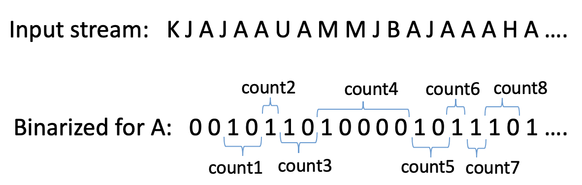
(a) An example sequence and its binary version for $A$.

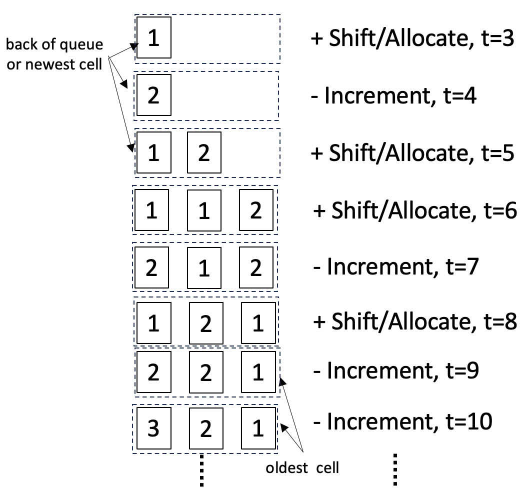
(b) Contents of q($A$) at a few times.

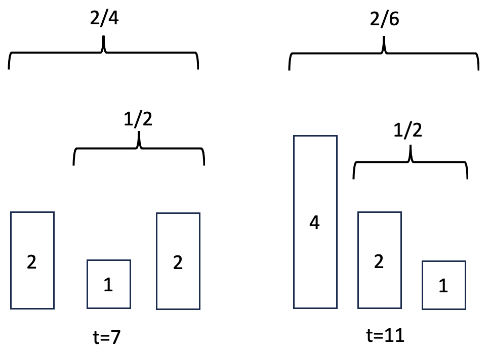
(c) Cells (counts) yield probabilities.

Figure 9: Illustrating the workings of the queues technique for tracking the probability of a single item: An example sequence (top, (a)), made binary for item $A$ (bottom), i.e. whenever A occurs, the entry in the binarized sequence is a 1, leading to a positive update of the queue, otherwise it is a 0, leading to a negative update (once the queue is allocated). Part (b) shows another view of the queue for $A$ upon queue creation and the first few updates (horizontal at each time point, left (newest cell, cell0) to right-most (oldest, cellk). At $t=3$ when the first $A$ is observed (the first positive update), the queue for $A$ is created with cell0 (newest cell of the queue), initialized with count 1. At time $t=4$ a negative update is performed and cell0 (its counter) is incremented. At $t=5$, another positive update, existing cell0 (its count content) is shifted one position to right, and a new cell0 is allocated with value 1, becoming the new back of the queue. More generally, on positive updates, existing cells shift to right and a new cell0 with an initial count of 1 is allocated, and on negative updates, the existing cell0 is incremented. At $t=8$, the value in cellk is discarded upon another positive update (assuming capacity 3), and so on. (c) Cell counts, shown at two snapshots, can be used to estimate a probability. There are several options for pooling the cells to get a probability. For instance, the back (left-most) partial cell can be ignored (see Section 5.4).

5.5 Predicting with SDs

Each queue in $qMap$ provides a PR for its item, but the PRs over all the items in a map may sum to more than 1 and thus violate the SD property. For instance, take the sequence $A$$A$$A$$A$$B$$B$$B$$B$ (several consecutive $A$s followed by several $B$s), and assume qcap $=3$: after processing this sequence, the PR for $B$ is 1.0, while for $A$ is $\frac{2}{6}$. See also Appendix C.3. The SD property is important for down-stream uses of the PRs provided by a method, such as computing expected utilities (and for a fair evaluation under KL() divergence). For evaluations, we apply the FC() function in Fig. 3(a) which works to normalize (scale down) and convert any input map into an SD as long as the map has non-negative values only.

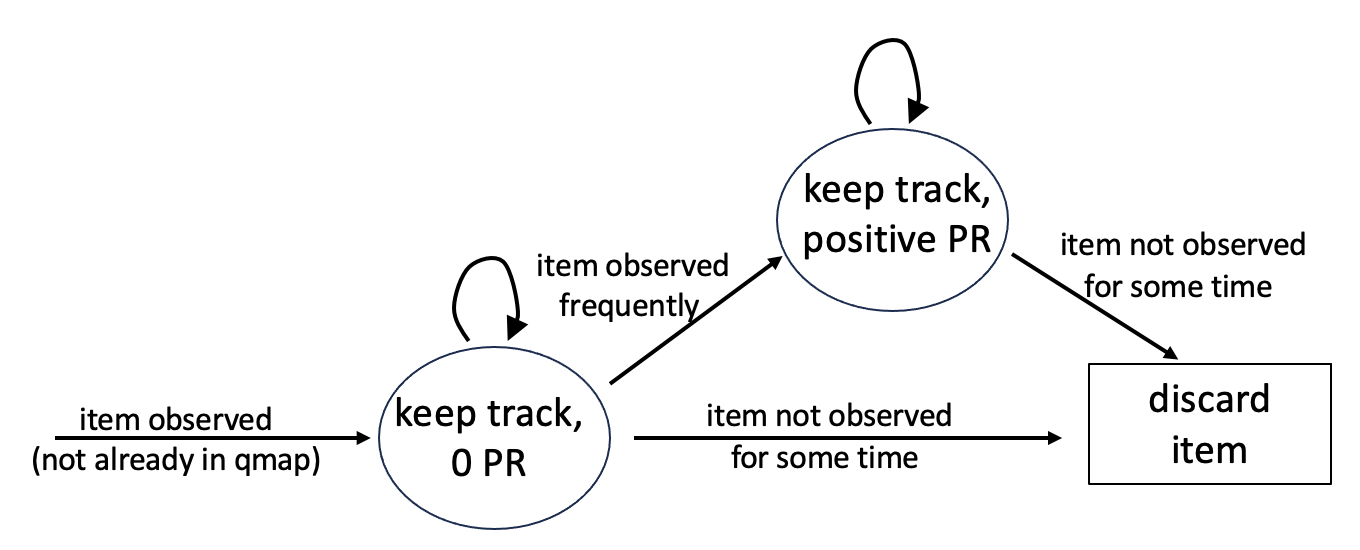
PruneQs($qMap$) // Pruning: A heart-beat method.

// Parameters: size & count limits $s_{1}$ and $s_{2}$,

//   such as $s_{1}=100$ and $s_{2}=10^{5}$.

Drop any item with $C_{0}>s_{2}$ from $qMap$

If $|qMap|<2s_{1}$:

Return // Nothing left to do.

Drop highest $C_{0}$ counts until $|qMap|$ is $s_{1}$.

Figure 10: Left: The possible state changes of an item as it enters $qMap$. The Qs technique keeps track of any item it sees in its stream, each for some (minimum) time. An item may also become salient (positive PR) and stay in that state indefinitely, or eventually discarded. Right: The pruning logic: items with large $C_{0}$ (count in cell0) are discarded. If the map is too large, it is pruned too (again, rank and remove by descending $C_{0}$, see Sect. 5.6).

The following properties hold, the proof of which (Lemma 8) along with other properties of the PRs , are in Appendix C.3. Below, $Q()$ is the PR map output of the Qs technique, or $Q(i)$ is the PR obtained from GetPR() when the queue for item $i$ is passed to it.

Lemma 4.

For the Qs technique with qcap $\geq 2$, for any item $i$ with a queue $q(i)$, $|q(i)|\leq$ qcap, using the PR estimate $Q(i)=(|q(i)|-1)/(\sum_{0\leq j<|q(i)|}C_{j}-1)$, for any time point $t\geq 1$:

1. $Q^{(t)}(i)$, when nonzero, has the form $\frac{a}{b}$, where $a$ and $b$ are integers, with $b\geq a\geq 1$.

2. If $i$ is observed at $t$, then $Q^{(t+1)}(i)\geq Q^{(t)}(i)$. If $i$ is not observed at $t$, then $Q^{(t+1)}(i)<Q^{(t)}(i)$.

5.6 Managing Space Consumption

There can be many infrequent items and the queues map of a predictor can grow unbounded, wasting space and slowing the update times, if a hard limit on the map size is not imposed. The size can be kept in check via removing the least frequent items from the map every so often, for instance via a method that works like a "heart-beat" pattern: map expansion continues until the size reaches or exceeds a maximum allowed capacity $2s_{1}$, e.g. $s_{1}=100$, remove the items in order of least frequency, i.e. rank by descending count $C_{0}$ in cell0 in each queue, until the size is shrunk back to $s_{1}$. When we are interested in modeling (tracking) probabilities down to a smallest PR $P_{min}$, in general we must have $s_{1}>\frac{1}{P_{min}}$ (e.g. with $p_{min}=0.01$, $s_{1}$ needs to be above 100). The higher $s_{1}$, the less likely that we drop salient items, i.e. items with (true) PR above $P_{min}$ (when a true PR exists, under the stationary setting). Note that those queues that are dropped, their PR when normalized, must be below $P_{min}$ whenever $s_{1}>\frac{1}{P_{min}}$, and the normalized PR is what we use when we want to use predictions that form a SD . Appendix C.3 explores the maximum possible number of PRs above a threshold before normalizing.

The above periodic pruning logic can also limit the count values within each queue, in particular in cell0, but not in the worst-case: imagine $A$ is seen once, and from then on $B$ is observed for all time. Thus $|qMap|=2$, and the above pruning logic is never triggered, while the count for $A$ in its cell0 can grow without limit (log of stream size). Thus, we can impose another constraint that if cell0 $C_{0}$ count-value of a queue in the $qMap$  is too large (e.g. $\frac{1}{C_{0}}\leq 10^{-4}$), such a queue (item) is removed as well. The trigger for the above checks can be periodic, as a function of the update count of the predictor (Fig. 8). The pruning logic is given in Fig. 10 (right).

Fig. 10, left, summarizes the states and state transitions of Qs upon observing an item not already in $qMap$, as it pertains to the item. Any item seen will be kept track of in $qMap$ for some time (assuming $s_{1}>1$). Being tracked does not imply positive PR (salience), however, if the item is seen more, it becomes salient (we require a minimum of two observations). It may also be discarded without ever becoming salient, or discarded after becoming salient. It may also enter the map and never exit.

5.7 Complexity of the Qs Method

Let $k=qcap$. At each time point, prediction using the qMapand update take the same $O(k|qMap|)$, where we assume $O(1)$ time for summing numbers and taking ratios: queue update involves updating the queue of every item in the map, and the updates, whether positive or negative, take $O(k)$ time. In our experiments, qcap $k$ is small, such as $3$ or $5$. With a $P_{min}$ of $0.01$ and periodic pruning of the map, the size of the queue for each predictor can grow to up to a few 100 entries at most.

Number of time steps required for estimating a PR output for an item with underlying PR ${p^{*}}$ (at the start of a new stable period), similar to EMA with harmonic decay (Sect. 4.3), is $\theta(\frac{1}{{p^{*}}})$ (time complexity).

5.8 A Time-Stamp Queuing Method for Global Sparse Updates

A close variant of the above Qs approach is what we can name the time-stamp method, which we now briefly sketch. In this version, each predictor keeps a single counter, or its own private clock. Upon an update, the predictor increments its clock. Nothing is done to the queues of items not observed (thus, a sparse update). For the observed item, a new cell0 is allocated as before and the current clock value is copied into it (instead of being initialized to 1, which was the case for plain Qs). Existing cells of this queue, if any, are shifted right, as before. Thus each queue cell simply carries the value of the clock at the time the cell was allocated, and the difference between consecutive cells is in effect the count of negative outcomes (the gaps), from which proportions can be derived.

When predicting, any item with no queue or a single-cell queue in $qMap$, gets 0 PR, as before. An item with more than one cell gets a positive PR, using a close variant of the GetPR() function of Fig. 8. The count corresponding to a queue is the current clock value minus the clock value of cellk (the oldest queue cell). The count is guaranteed to be positive, and is equivalent to the denominator used in GetCount(). Then the PR is the ratio of number of cells in the item’s queue, $k$, to its count.

This variation has the advantage that updating is O(1) only with the mild assumption that Qs operations and counting take constant time (i.e. incrementing clock and the operations on a single item’s queue), while for the plain Qs technique, recall that it is $O(|qMap|)$. In this sense, this extension is strictly superior. However, during prediction, if that involves predicting all items’ PRs in the map, complexity remains $O(|qMap|)$, so within the online cycle of predict-observe-update, time costs would not change asymptotically. However, the time-stamp variant is useful in scenarios where, instead of asking for all PRs, one queries for the probability of one or a few items only, e.g. when one seeks the (approximate non-stationary) prior of a few items. In particular, when the number of items for which one seeks to keep a prior for is large, e.g. millions (thus, we are interested in estimating small probabilities, such as $p\leq 10^{-6}$), a sparse update is attractive.

5.8.1 Counting Overflow

Incrementing the clock with each update can lead to large clock values (log of stream length) and require significant memory for a predictor that frequently updates. One can manage such, and in effect limit the window size and the prediction capacity, i.e. the number of items for which an approximate PR is kept at any point, by periodically pruning and shifting the update count value to a lower value.

6 DYAL: EMA and Qs, Combined

The basic idea here is that the Qs technique can give us a good roughly unbiased starting point for an estimate of the PR of an item, but it has a high variance unless much queue space is used. With EMA, and with our assumption that there will be periods of stability, and when the Qs estimate indicates that the item can be salient, we can fine tune this estimate with less space using two parameters, a weight (the PR) and a learning rate, and via EMA’s logic. Similarly, the queues can tell us when an item should be discarded, or more generally when the PR of an item should be substantially reduced. Finally, the queues also provide a good starting learning rate for EMA’s use.

Thus we use a combination of EMA and the Qs technique. The queues are used as “gates”, the interface to the external observed stream, playing a major role in determining what is kept track of and what is discarded, and providing rough initial estimates, of the PR and $\beta$, whenever the PR of an item needs to substantially change.

We refer to this hybrid technique as DYAL, for dynamic adjustment of the learning (rate), with the mnemonic of dialing up and down the learning. In order to achieve this, DYAL, for every predictand that it keeps track of, maintains a small queue, and a learning rate, in addition to the PR (a weight). Fig. 11 shows the pseudo code for the major functions. Like EMA, DYAL has a map for the PR weights, $EmaMap$, but it also has a (parallel) map of learning rates, $rateMap:$ item $\rightarrow\beta$, and similarly a map of (small) queues, $qMap$ (like Qs). The space overhead can therefore be thought of as a few extra bytes per predictor-predictand relation (per prediction edge, in addition to the bytes needed for the PR weight, in plain EMA).

Predicting in DYAL is like plain EMA: use $EmaMap$. It is ensured that the map always remain a SD when updating. Updating involves both an EMA-like update, weakening EMA edges and (possibly) strengthening one, and a Qs update: all the three maps are updated, as given in the UpdateDyal() function. Upon each observation $o$, first the queues information on $o$ is obtained. This is the current queue probability $qPR$ (possibly 0) on $o$, and the $qcount$ (invoke GetCount()). Then $qMap$ is updated (a Qs-type update). Finally, all the edges in the EMA map, except for $o$, are weakened. If there was no queue for $o$, i.e. when $qPR$ is 0, $o$ must be new, or NS in general, and nothing more is done, i.e. no edge strengthening is done (note that a queue is allocated for $o$ upon the $qMap$ update). Weakening, for each edge, is either a plain EMA weakening, or the queue estimates are used, which we cover next. Similarly, for strengthening, the condition for switching to queues is tested and the appropriate strengthening action is taken.

UpdateDyal($o$) // latest observation $o$.

// Data structures: $qMap$, $EmaMap$, $rateMap$.

$qPR,qcount\leftarrow$ GetQinfo($qMap,o$)

UpdateQueues($qMap$, $o$)

$free\leftarrow$ WeakenEdges($o$) // Weaken, except for $o$.

If $qPR$ == $0$: // item is currently NS?

Return

$emaPR\leftarrow$ $EmaMap.get(o,0.0)$ // 0 if $o\not\in$ Map.

// listen to queue?

If Q_SignificantlyHigh($emaPR,qPR,qcount$):

$rateMap[o]\leftarrow qcount^{-1}$ // set to q info.

$\delta\leftarrow\min(qPR-emaPR,free)$

Else:

$\beta\leftarrow rateMap[o]$

$\delta\leftarrow\min((1-emaPR)*\beta,free)$

$rateMap[o]\leftarrow DecayRate(\beta)$

$EmaMap[o]\leftarrow\delta+emaPR$

Q_SignificantlyHigh($emaPR,qPR,qcount$)

// Parameter: $sig\_thrsh$ (significance threshold).

If $emaPR==0$: // when 0, listen to Qs .

Return True

If $qPR\leq emaPR$:   Return False

Return $qcount*KL(qPR,emaPR)\geq sig\_thrsh$

Q_SignificantlyLow($emaPR,qPR,qcount$)

// Parameter: $sig\_thrsh$ (significance threshold).

If $emaPR\leq qPR$:   Return False

Return $qcount*KL(qPR,emaPR)\geq sig\_thrsh$

WeakenEdges($o$) // Weaken and return available mass

// Data structures: $qMap$, $EmaMap$, $rateMap$.

// Parameter: $P_{min}$.

// Weaken all except for $o$. Returns the free mass.

$used\leftarrow 0$

For each item and learning-rate, $i$, $\beta$ in $rateMap$:

If $i==o$: // Don’t weaken $o$

$used\leftarrow used+EmaMap[o]$

Continue

// Possibly listen (switch) to the queue.

$qPR,qcount\leftarrow$ GetQinfo($qMap,i$)

// if too low, drop $i$

If $\max(EmaMap[i],qPR)<P_{min}$:

$EmaMap$.delete(i) & $rateMap$.delete(i)

Continue // remove item and go to next.

If Q_SignificantlyLow($EmaMap[i],qPR,qcount$):

$EmaMap[i]\leftarrow qPR$ // set to q info.

$rateMap[i]\leftarrow qcount^{-1}$

Else: // weaken as usual

$EmaMap[i]\leftarrow(1-\beta)*EmaMap[i]$

$rateMap[i]\leftarrow DecayRate(\beta)$

$used\leftarrow used+EmaMap[i]$

Return $1.0-used$ // The free (available) mass

GetQInfo($qMap$, $o$)

If $o\notin qMap$: // no queue for $o$?

Return 0, 0

$q\leftarrow qMap$.get($o$)

Return GetPR($q$), GetCount($q$))

Figure 11: Pseudo code for DYAL. DYAL is an extension of plain sparse EMA where each predictand (or edge) has a small queue and its own learning rate, in addition to the PR estimate (a weight).

6.1 When and How to Listen to the Queues Estimate: Statistical Tests

The queue for each item provides two numbers, the number of cells of the queue is the implicit number of positives observed recently, and the total count across the queue cells is the number of trials (roughly, the GetCount() function). These numbers also provide a PR estimate $qPR$ (GetProb()). We also have an estimate of PR, emaPR, from the EMA weights $EmaMap$, which we expect to be generally more accurate with lower variance than $qPR$, but specially in the face of non-stationarity, from time to time this estimate could be out-dated. Based on the counts and the queue estimate $qPR$, we can perform a binomial-tail test that asks whether, when assuming $emaPR$ is the true PR, one can observe the alternative PR $qPR$ in $qcount$ trials, with some reasonable probability. This binomial tail can be approximated (lower and upper-bounded) efficiently in $O(1)$ time when one has the number of trials and the observed PR $qPR$ [2, 3, 27], and it tells us how likely it is that a binary event with assumed true PR $emaPR$ could lead to the counts and the qPR estimate (of the queue). As seen in Fig. 11, the approximation is based on the (binary) KL divergence ($\mbox{KL}(qPR||emaPR)$). When this event is sufficiently unlikely, or, equivalently, when the binomial-tail score is sufficiently high, DYAL switches to the queue estimate and sets the new rate $\beta$ accordingly too. By default we use a score threshold of 5, corresponding to 99% confidence. In a few experiments, we report on sensitivity of DYAL to the choice of the binomial threshold.

6.2 SD Maintenance and Convergence

We can verify from the logic of DYAL, i.e. the weakenings and strengthening of the weights and the bounding of $\delta$ (the PR to add) by the $free$ variable (the available, or unallocated, PR mass), that the $EmaMap$ of DYAL always corresponds to an SD: the PR values kept are positive and never sum to more then 1.0. In the stationary setting, the properties of plain EMA apply and the PRs should coverge to the true PRs, except there is some low probability that once in a while switching to the queue may occur with a more variant estimate. We leave a more formal analysis to future work.

6.3 Pruning (Space Management) and Asymptotic Complexity

The pruning logic for the three maps of DYAL is identical to the logic for pruning for the Qs method of Sect. 5.6 except that when an entry is deleted from the queue, its corresponding entries (key-value pairs) in $rateMap$  and $EmaMap$  are also deleted when they exist. Thus the set of keys in the $qMap$  of the predictor will always be a superset of the key sets in $rateMap$  and $EmaMap$ (note: the keysets in $rateMap$  and $EmaMap$ are always kept identical). The size of $EmaMap$ does not exceed $O(\frac{1}{P_{min}})$ as it is a SD, and $qMap$ is prunned periodically as well. Updating time cost for DYAL is similar to Qs: each edge (predictand) is examined and the corresponding queue and possibly EMA weights and learning rate are updated, each test and update (wearkening and boosting) take $O(1)$ (per edge) where we assume qcap is constant, and update and prediction take $O(|qMap|)$ time.

6.4 Discussion: Why not multiple EMAs with different rates?

Why can’t we use two (or more) tiers of EMA, one with high fixed rate, so agile and adaptive, another with a low and fixed rate, so stable for fine tuning, rather than our current proposed hybrid two-tier approach in DYAL that also uses queues and predictand-specific $\beta$s? Queues are an effective way to differentiate between noise items (below $P_{min}$) from salient items (with good likelihood of success). On the other hand, EMA with a high fixed rate $\beta$ is too coarse (non-differentiating) for learning PRs below the $\beta$.

It may be possible to use multiple non-fixed rate “scanning” EMAs, where the learning rate for each scanner is reset to high but decreased over time (such as via harmonic decay), to achieve similar goals. We leave this to future work.

7 Synthetic Experiments

We begin with the synthetic experiments, wherein we generate sequences knowing the true SDs $\mathcal{P}^{(t)}$. At any time point, for evaluation, the FC() function of Fig. 3 is applied to the output of all predictors, with $P_{NS}=P_{min}=0.01$. The default parameters for DYAL are qcap of 3 and binomial-tail threshold of $5$, and we report the performance of DYAL for different $\beta_{min}$, often set at 0.001. We are interested in $\beta_{min}\leq 0.001$ because our target range is learning PRs in $[0.01,1.0]$ well. For static EMA, we report the (fixed) $\beta$ used, for harmonic EMA, the $\beta_{min}$, and for Qs, the qcap. All code is implemented in Python, and we report timing for several of the experiments (those taking longer than minutes).

7.1 Tracking a Single Item, Stationary

All the prediction techniques are based on estimating the probability (PR) for each item separately (treating all other observations as negative outcomes), so we begin with assessing the quality of the predictions for a single item in the binary stationary setting of Sect. 2.1.3. Thus, when ${p^{*}}=0.1$, about $10\%$ of the sequence is 1, the rest 0. Table 4 presents the deviation rates of Qs, EMA, and DYAL, under a few parameter variations, and for ${p^{*}}\in\{0.1,0.05,0.01\}$. Sequences are each 10k time points long, and deviation rates are averaged over 200 such sequences.

Under this stationarity setting, higher qcap helps the Qs technique: Qs with qcap 10 does better than qcap of 5, but, specially for $d=1.5$, both tend to substantially lag behind the best of the EMA variants. EMA with harmonic decay, with an appropriately low $\beta_{min}$, does best across all ${p^{*}}$. If we anticipate that the useful items to predict will have PRs in the $0.01$ to $1.0$ range, in a stationary world, then setting $\beta_{min}$ for harmonic EMA to a low value, $\frac{0.01}{k}$, where $k\geq 10$, is adequate. In this stationary and binary setting, the complexity of DYAL is not needed, and harmonic EMA is sufficient. Still DYAL is the second best. Static EMA is not flexible enough, and one has to anticipate what ${p^{*}}$ is and set the rate appropriately. For instance, when ${p^{*}}=0.01$, EMA with the same $\beta=0.01$ is not appropriate, resulting in too much variance. Finally, we observe that the deviation rates, as well as the variances, for any method, degrade (increase) somewhat as ${p^{*}}$ is lowered from $0.1$ to $0.01$. In ten thousand draws (during sequence generation), there are fewer positive observations with lower ${p^{*}}$, and estimates will have higher variance (see also Appendix C.1).

deviation$\rightarrow$	1.5	2	1.5	2
threshold	Qs, qcap of 5		Qs, qcap of 10
${p^{*}}=0.10$	0.385 $\pm$ 0.026	0.129 $\pm$ 0.020	0.191 $\pm$ 0.029	0.026 $\pm$ 0.010
${p^{*}}=0.05$	0.405 $\pm$ 0.034	0.142 $\pm$ 0.028	0.211 $\pm$ 0.044	0.035 $\pm$ 0.016
${p^{*}}=0.01$	0.435 $\pm$ 0.078	0.169 $\pm$ 0.065	0.256 $\pm$ 0.095	0.064 $\pm$ 0.044
	static EMA, $\beta$ of 0.01		static EMA, $\beta$ of 0.001
${p^{*}}=0.10$	0.075 $\pm$ 0.021	0.013 $\pm$ 0.006	0.113 $\pm$ 0.020	0.071 $\pm$ 0.012
${p^{*}}=0.05$	0.211 $\pm$ 0.034	0.050 $\pm$ 0.019	0.118 $\pm$ 0.029	0.072 $\pm$ 0.016
${p^{*}}=0.01$	0.596 $\pm$ 0.032	0.373 $\pm$ 0.040	0.182 $\pm$ 0.083	0.091 $\pm$ 0.047
	harmonic EMA, $\beta_{min}$ of 0.001		DYAL , $\beta_{min}$ of 0.001
${p^{*}}=0.10$	0.006 $\pm$ 0.007	0.002 $\pm$ 0.003	0.018 $\pm$ 0.015	0.008 $\pm$ 0.006
${p^{*}}=0.05$	0.012 $\pm$ 0.013	0.005 $\pm$ 0.005	0.028 $\pm$ 0.023	0.014 $\pm$ 0.012
${p^{*}}=0.01$	0.118 $\pm$ 0.078	0.029 $\pm$ 0.029	0.155 $\pm$ 0.093	0.057 $\pm$ 0.044

Table 4: Synthetic single-item stationary: Deviation rates, for two deviation thresholds $d\in\{1.5,2\}$, averaged over 200 randomly generated sequences of 10000 binary events (0 or 1), for target probability ${p^{*}}\in\{0.01,0.05,0.1\}$. As an example, for ${p^{*}}=0.1$, about $10\%$ of the items will be 1, the rest are 0s in the sequence, and the predictor predicts a probability $\hat{p}^{(t)}$ at every time point $t$ for $o^{(t)}=1$ (then updates), and we observe from the table that about $38\%$ of time, $\max(\frac{\hat{p}^{(t)}}{p},\frac{p}{\hat{p}^{(t)}})>1.5$ (i.e. $\hat{p}^{(t)}>0.15$ or $\hat{p}^{(t)}<\frac{0.1}{1.5}$), for the Qs predictor with qcap 5 (top left). The lower the deviation rates the better. In this stationary setting, we see improvements with larger queue capacities (as expected), and a lower $\beta_{min}$ of 0.001 performs best for the EMA variants. For the Qs technique, with qcap $=10$, compare to Table 3 under $t_{p}=10$.

7.2 Tracking a Single Item, Non-Stationary

deviation $\rightarrow$	1.5	2	1.5	2
threshold	Qs, 5		Qs, 10
0.025 $\leftrightarrow$ 0.25, 10	0.423 $\pm$ 0.029	0.189 $\pm$ 0.023	0.395 $\pm$ 0.021	0.234 $\pm$ 0.014
0.025 $\leftrightarrow$ 0.25, 50	0.382 $\pm$ 0.038	0.131 $\pm$ 0.028	0.222 $\pm$ 0.039	0.062 $\pm$ 0.017
$\mathcal{U}(0.01,1.0)$, 10	0.429 $\pm$ 0.030	0.207 $\pm$ 0.024	0.483 $\pm$ 0.028	0.296 $\pm$ 0.028
$\mathcal{U}(0.01,1.0)$, 50	0.361 $\pm$ 0.038	0.128 $\pm$ 0.028	0.224 $\pm$ 0.040	0.074 $\pm$ 0.017
	static EMA, 0.01		static EMA, 0.001
0.025 $\leftrightarrow$ 0.25, 10	0.510 $\pm$ 0.024	0.357 $\pm$ 0.020	0.996 $\pm$ 0.006	0.760 $\pm$ 0.043
0.025 $\leftrightarrow$ 0.25, 50	0.255 $\pm$ 0.045	0.129 $\pm$ 0.028	0.705 $\pm$ 0.032	0.560 $\pm$ 0.023
$\mathcal{U}(0.01,1.0)$, 10	0.686 $\pm$ 0.030	0.477 $\pm$ 0.035	0.818 $\pm$ 0.038	0.693 $\pm$ 0.054
$\mathcal{U}(0.01,1.0)$, 50	0.397 $\pm$ 0.056	0.209 $\pm$ 0.045	0.775 $\pm$ 0.085	0.602 $\pm$ 0.099
	Harmonic EMA, 0.01		Harmonic EMA, 0.001
0.025 $\leftrightarrow$ 0.25, 10	0.502 $\pm$ 0.025	0.351 $\pm$ 0.021	0.957 $\pm$ 0.021	0.668 $\pm$ 0.053
0.025 $\leftrightarrow$ 0.25, 50	0.247 $\pm$ 0.046	0.123 $\pm$ 0.028	0.606 $\pm$ 0.031	0.494 $\pm$ 0.018
$\mathcal{U}(0.01,1.0)$, 10	0.684 $\pm$ 0.033	0.476 $\pm$ 0.034	0.813 $\pm$ 0.036	0.683 $\pm$ 0.050
$\mathcal{U}(0.01,1.0)$, 50	0.395 $\pm$ 0.056	0.204 $\pm$ 0.043	0.761 $\pm$ 0.079	0.592 $\pm$ 0.097
	DYAL, 0.01		DYAL, 0.001
0.025 $\leftrightarrow$ 0.25, 10	0.480 $\pm$ 0.029	0.332 $\pm$ 0.025	0.586 $\pm$ 0.066	0.408 $\pm$ 0.061
0.025 $\leftrightarrow$ 0.25, 50	0.251 $\pm$ 0.048	0.150 $\pm$ 0.031	0.099 $\pm$ 0.066	0.053 $\pm$ 0.037
$\mathcal{U}(0.01,1.0)$, 10	0.585 $\pm$ 0.035	0.362 $\pm$ 0.034	0.566 $\pm$ 0.052	0.350 $\pm$ 0.045
$\mathcal{U}(0.01,1.0)$, 50	0.319 $\pm$ 0.065	0.140 $\pm$ 0.049	0.301 $\pm$ 0.081	0.153 $\pm$ 0.049

Table 5: Synthetic single-item non-stationary: Deviation-rates on sequences where ${p^{*}}$ oscillates back and forth between 0.025 and 0.25, or drawn uniformly at random from the interval $[0.01,1.0]$ (${p^{*}}\sim\mathcal{U}(0.01,1.0)$). Each sequence is 10k observations long, and the deviation-rate is averaged over 500 such sequences. For the case of 0.025 $\leftrightarrow$ 0.25, each subsequence (wherein ${p^{*}}$ is constant) is roughly same length: 400 long for $O_{min}=10$, and 2k for $O_{min}=50$. For the rows with $\mathcal{U}(0.01,1.0)$, each subsequence is at least 1k (and has to meet the $O_{min}$ constraint too) (see 7.2 text for details).

We continue with tracking a single item as above, as we report deviation rates when estimating a single ${p^{*}}$, but now the predictors face non-stationarity. As in the above, sequences of 10000 items are generated in each trial. We report on two main settings for non-stationarity: In the first setting, ${p^{*}}$ oscillates between, 0.25 and 0.025, thus an abrupt or substantial change (10x) is guaranteed to occur and frequently. This oscillation is shown as $0.25\leftrightarrow 0.025$ in Table 5. In the second ’uniform’ setting, each time ${p^{*}}$ is to change, we draw a new ${p^{*}}$ uniformly at random from the interval $[0.01,1.0]$, shown as $\mathcal{U}(0.01,1.0)$, and in this setting, some changes are large, others small and could be viewed as drifts. The stable period, during which ${p^{*}}$ cannot change (to allow time for learning), is set as follows. For both settings, within a stable period, the target item (item 1) has to be observed at least $O_{min}$ times (a positive outcome, 1, observed for $O_{min}$ times), before ${p^{*}}$ is eligible to change, where results for $O_{min}\in\{10,50\}$ are shown in Table 5. Additionally, we impose a general minimum-length constraint (not just on positive observations) for the $0.25\leftrightarrow 0.025$ setting, each stable period has to be $\frac{O_{min}}{\min(0.025,0.25)}$, so that the different periods would have similar length (expected 400 time points when $O_{min}=10$, and 2000 when $O_{min}=50$). In this way, subsequences corresponding to ${p^{*}}=0.25$ would not be too short (otherwise, deviation-rate performance when ${p^{*}}=0.025$ dominates). Thus, with $0.25\leftrightarrow 0.025$, we get an expected 25 stable subsequences (or changes in ${p^{*}}$) in 10k long sequences with $O_{min}=10$, and 5 switches in ${p^{*}}$ when $O_{min}=50$. For the uniform setting, we did not impose any extra constraint, and respectively with $O_{min}$ of 10 and 50, we get around 200 and 50 stable subsequences in 10k time points. In this setting, performances in periods when ${p^{*}}$ is low do dominate the deviation rates (see also Table 15 where the deviation-rates improve when we impose an overall minimum-length constraint for the uniform setting too).

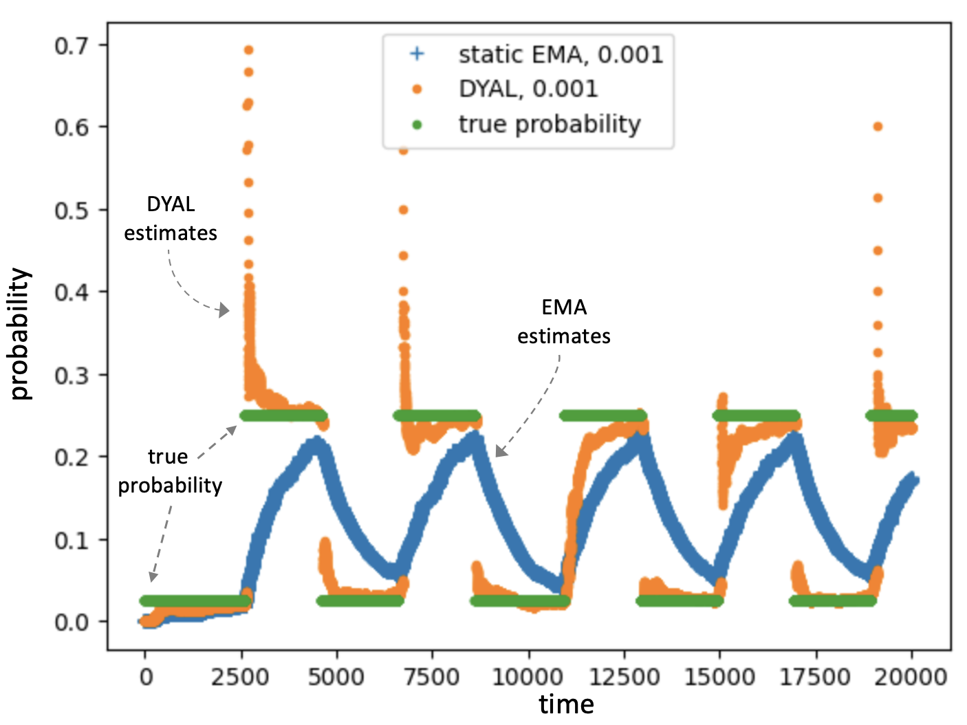
(a) Min-Rate of 0.001

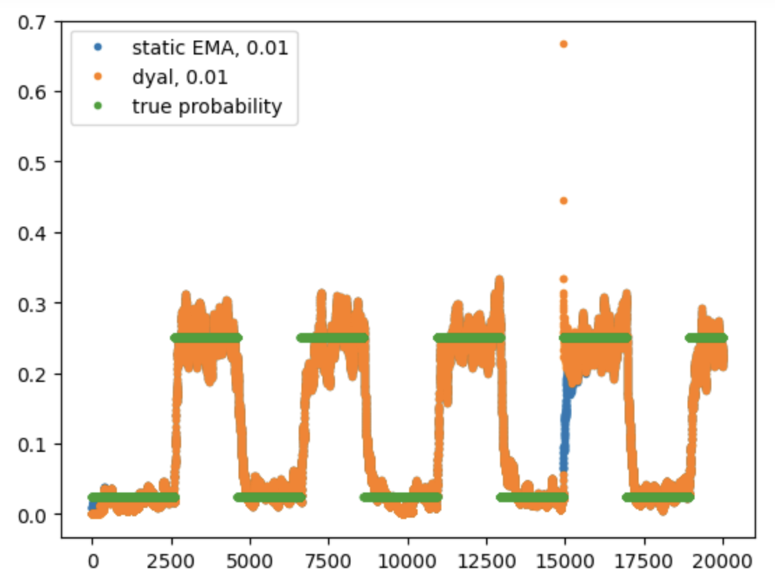
(b) Min-Rate of 0.01

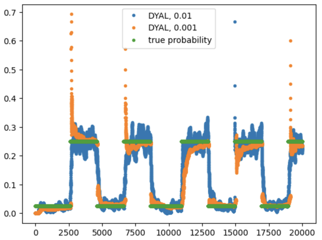
(c) DYAL Min-Rate of 0.001 vs 0.01

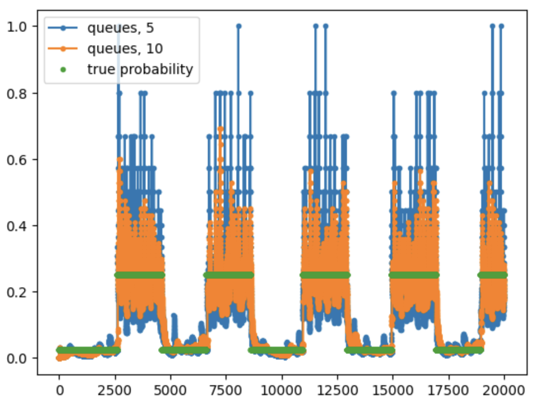
(d) Qs with capacity 5 and 10.

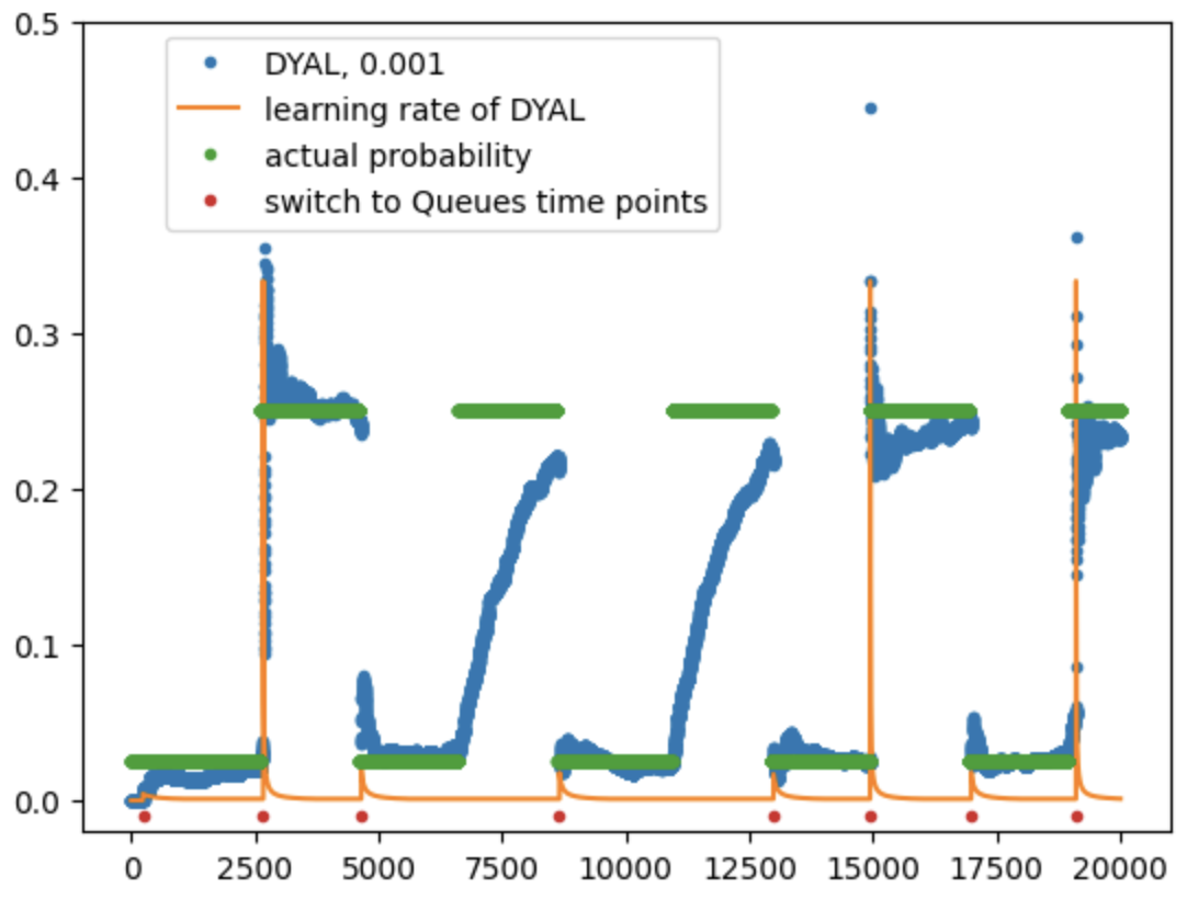
(e) Changes in the learning rate $\beta$.

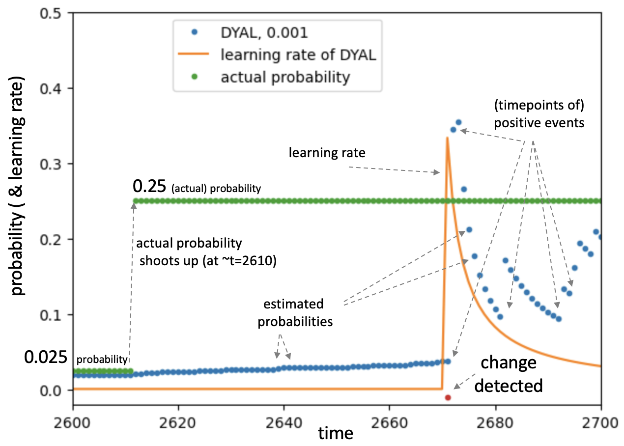
(f) A close up of change in $\beta$.

Figure 12: Synthetic single-item oscillation experiments, 0.025 $\leftrightarrow$ 0.25, on a single sequence. Parts (a) to (d) show the estimates of the three predictors, EMA, Qs, and DYAL, blue and orange colors, around the true probability (green, up-down steps). We can assess convergence speed and variance. Parts (e) and (f) also show evolution of the learning rate and the rate hikes as the probability of a single event is tracked via DYAL.

Compared to the results of Table 4, here the Qs predictor excels, specially when we consider deviation-rates when $O_{min}$=10. With such non-stationarity, qcap =5 can even work better than qcap =10 (unlike the previous section). In this non-stationary setting, DYAL is the 2nd best, and performs substantially better than the other EMA variants. $O_{min}$ of 10 may still be considered on the low side (i.e. relatively high non-stationarity). With $O_{min}=50$, first off, every technique’s deviation-rate improves, compared to $O_{min}$=10 setting. DYAL, with $\beta_{min}$=0.001, performs best for the $0.25\leftrightarrow 0.025$ and Qs, qcap =10, works best with uniform ${p^{*}}$, DYAL remaining second best. When picking from uniform, the change in $p$ may not be high, Qs can pick up such change faster, and more naturally, than DYAL, which performs explicit tests and may or may not raise its learning rate depending on the extent of change. However, Qs with 10, despite its simplicity, does require significant extra memory.

Figs. 12 shows plots of the output estimates $\hat{p}^{(t)}$, along one of the oscillating sequences ($0.25\leftrightarrow 0.025$). As expected, we observe that the Qs technique leads to high variance during stable periods, qcap of 5 substantially higher than qcap of 10 (Fig. 12(d)). Similarity for both (static) EMA and DYAL, the rate of 0.01 exhibits higher variance than 0.001 (Figs. 12(b) and (c)). Static EMA and DYAL with 0.01 are virtually identical in Fig. 12(b), except that DYAL can have discontinuities when ${p^{*}}$ changes (when it listen to its queue estimates, as discussed next), and converges from both sides of the target ${p^{*}}$, while plain EMA converges from one side.

Fig. 12(e) shows the evolution of the learning rate of DYAL, and in particular when DYAL detects a (substantial or sufficiently significant) change (shown via red dots close to the x-axis). At the scale shown, rate increases look like pulses: they go up (whenever DYAL listens to a queue) and then with harmonic decay, they fairly quickly come back down (resembling spikes at the scale of a few hundred time points, for PRs in $[0.01,1.0]$). We also note that this rate increase can happen when a high probability (0.25) changes to a low probability (0.025) as well, though the rate increase is not as large, as would be expected. We also note that DYAL is not perfect in the sense that not all the changes are captured (via switching to its queues’ estimates), in particular, there are a few “false negatives”, when a change in ${p^{*}}$ occurs in the sequence and DYAL continues to use its existing learning rates and adapt its existing estimates. This may suffice when the $\beta$ at the time is sufficiently high or when the estimate is close. In particular, we can observe in Figs. 12(b) and (c) that a higher rate, $\beta_{min}=0.01$, leads to fewer switches compared to 0.001, and in Figs. 12(b) we observe that DYAL behaves almost identically to static EMA when both have $0.01$ (there appears to be one switch only at $t=15000$ for DYAL).

Fig. 12(f) presents a close up of when a (significant) change is detected and a switch does occur, from a low true probability of ${p^{*}}=0.025$ to ${p^{*}}=0.25$ in the picture. Note that before the switch, the estimates (the blue line) start rising, but this rise may be too slow. Once sufficient evidence is collected, both the estimate and the learning rate are set to the queues’ estimate, which is seen as a more abrupt or discontinuous change in the picture. The estimates then more quickly converge to the new true PR of 0.25. While we have not shown the actual negative and positive occurrences in the picture, it is easy to deduce where they are from the behavior of $\hat{p}^{(t)}$ (specially after the switch, where the estimates are high): the positives occur when there is an increase in the estimate $\hat{p}^{(t)}$ (from $t$ to $t+1$). Fig. 18 and Fig. 24 show additional patterns of change in the learning rate in multi-item real sequences.

Appendix D reports on a few additional variations in parameters and settings, e.g. Qs with qcap =3, and deviation threshold $d=1.1$, as well as imposing a minimum-length constraint for the uniform setting (Tables 14 and 15).

There are additional challenges (e.g. of setting appropriate parameters), when a predictor has to predict multiple items well, with different items having different probabilities and exhibiting different non-stationarity patterns. This is the topic of the next section and the rest of the paper.

7.3 Synthetic, Non-Stationary, Multi-Item

GenSequence($desiredLen,O_{min},L_{min}$)

// Create & return a sequence of subsequences.

$seq\leftarrow$ [] // A sequence of items.

$prevSD\leftarrow\{\}$

While len($seq$)$<desiredLen$:

// Extend existing sequence

$\mathcal{P}\leftarrow$ GenSD($prevSD$)

$seq$.extend(GenSubSeq($\mathcal{P}$), $O_{min},L_{min}$))

$prevSD\leftarrow\mathcal{P}$

Return $seq$

GenSubSeq($\mathcal{P},O_{min},L_{min}$)

// Generate a stable/stationary subsequence, via repeated

// sampling iid from SD $\mathcal{P}$. It should be long enough that

// every item in $\mathcal{P}$ occurs $\geq O_{min}$ times in it.

$counts\leftarrow\{\}$ // An observation counter map.

$seq\leftarrow$ [] // A sequence of items.

While $\min(counts)<O_{min}$ or len($seq$) $<L_{min}$:

$o\leftarrow$ DrawItem($\mathcal{P}$) // item $o$ drawn.

seq.append(o)

// Update counts only for salient (non-noise) items.

If $o\in\mathcal{P}$: // increment o’s observed count.

$counts[o]\leftarrow counts.get(o,0)+1$

Return $seq$

GenSD($prevSD$)

// Parameters: $reuse,P_{min},P_{max},P_{NS}$.

$probs\leftarrow$ [] // Probabilities drawn for the distribution.

$left\leftarrow 1.0$ // Probability mass left to draw from.

While $left>P_{NS}+P_{min}$:

$p_{max}\leftarrow\min(left-P_{NS},P_{max})$

$p\sim\mathcal{U}([P_{min},p_{max}])$ // draw uniformly at random.

$probs$.append($p$)

$left\leftarrow 1.0-sum(probs)$

If $reuse$: // reuse items ’1’, ’2’, ..

Random.shuffle(probs) // random permute

// item ’1’ gets probs[0], ’2’ gets probs[1], etc.

Return MakeMap(probs)

Else: // Allocate new items (ids).

Return MakeNewSDMap($probs,prevSD$)

DrawItem($\mathcal{P}$) // Return (sample) a salient or noise item.

$sump\leftarrow 0.0$

$p\sim\mathcal{U}([0,1.0])$

For $o,prob\in\mathcal{P}$:

$sump\leftarrow sump+prob$

If $p\leq sump$:

Return $o$ // Done.

Return UniqueNoiseItem()

Figure 13: Pseudocode for generating a sequence of subsequences. Each subsequence corresponds to a stable period, subsequence $j\geq 1$ being the result of drawing iid from the $j$th SD, $\mathcal{P}^{(j)}$.

Fig. 13 provides pseudocode of the main functions for generating item (observation) sequences under non-stationarity. As in the above, we think of a non-stationary sequence as a concatenation of “stable” (stationary) subsequences, subsequence $j$, $j\geq 1$, corresponding to one SD $\mathcal{P}^{(j)}$. The subsequence is long enough (drawn iid from $\mathcal{P}^{(j)}$) so that $\min_{i\in\mathcal{P}^{(j)}}count(i)\geq O_{min}$, where $count(i)$ is the number of occurrences of item $i$ in the subsequence. We may have a minimum (overall) length requirement as well, $L_{min}\geq 0$. Each $\mathcal{P}^{(j)}$ is created using the GenSD function.

In GenSD, some probability, $P_{NS}$, is reserved for noise, the NS items. Probabilities are drawn uniformly from what probability mass is available, initially $1-P_{NS}$, with the constraint that each drawn probability $p$ should be sufficiently large, $p\geq P_{min}$. Optionally, we may impose a maximum probability $P_{max}$ constraint as well ($P_{max}<1$). Assume we get the set $S=\{p_{1},p_{2},\cdots,p_{k}\}$, once this loop in GenSD is finished, then we will have $\sum_{p_{i}\in S}p_{i}\leq 1-P_{NS}$, and each PR $p_{k}$ satisfies the minimum and maximum constraints.

	1.5any	1.5obs	logloss	1.5any	1.5obs	logloss	opt. loss
new items $\downarrow$	Qs, 5			Qs, 10
$O_{min}=10$	0.94	0.24	1.17	0.88	0.17	1.19	1.040 $\pm$0.11
$O_{min}=50$	0.92	0.22	1.13	0.78	0.10	1.09	1.028 $\pm$0.22
	static EMA, 0.01			static EMA, 0.001
10	0.86	0.20	1.26	1.00	0.95	2.33	1.040
50	0.80	0.06	1.07	0.70	0.32	1.44	1.028
	harmonic EMA, 0.01			harmonic EMA, 0.001
10	0.86	0.19	1.25	0.98	0.88	2.25	1.040
50	0.80	0.06	1.07	0.62	0.23	1.34	1.028
	DYAL, 0.01			DYAL, 0.001
10	0.94	0.09	1.11	0.89	0.09	1.14	1.040
50	0.89	0.05	1.05	0.59	0.03	1.06	1.028
recycle items $\downarrow$	Qs, 5			Qs, 10
$O_{min}=10$	0.91	0.23	1.16	0.83	0.13	1.14	1.040 $\pm$0.11
$O_{min}=50$	0.91	0.22	1.12	0.76	0.10	1.08	1.028 $\pm$0.22
	static EMA, 0.01			static EMA, 0.001
10	0.87	0.16	1.16	1.00	0.73	1.65	1.040
50	0.80	0.06	1.06	0.77	0.26	1.28	1.028
	harmonic EMA, 0.01			harmonic EMA, 0.001
10	0.87	0.15	1.15	0.98	0.66	1.54	1.040
50	0.80	0.05	1.05	0.71	0.18	1.18	1.028
	DYAL, 0.01			DYAL, 0.001
10	0.91	0.10	1.11	0.83	0.16	1.18	1.040
50	0.88	0.05	1.04	0.56	0.04	1.06	1.028

Table 6: Synthetic multi-item experiments: Deviation rates and log-loss, averaged over 50 sequences, 1̃0k length each, $O_{min}$ of 10 and 50, uniform SD generation vis GenSD(): $P_{max}=1.0$, $P_{min}=P_{NS}=0.01$ for GenSD(), and change the SD $\mathcal{P}$ whenever all salient items in $\mathcal{P}$ are observed $\geq O_{min}$ times. In top half, items are new when underlying SD changes, and in the bottom half, items are ’recycled’ (Sect. 7.3).

Once the set $S$ of $k$ PRs generated, GenSD() then makes a SD from $S$. Under the new-items setting (when $recycle=0$), new item ids, $|S|$ such, are generated, e.g. an item id count is incremented and assigned, and the items are assigned the probabilities (and all the old items, salient in $\mathcal{P}^{(j-1)}$, get zeroes, so discarded). Thus, the first few SDs could be $\mathcal{P}^{(1)}=\{$1:0.37, 2:0.55, 3:0.065$\}$, $\mathcal{P}^{(2)}=\{$4:0.75, 5:0.21, 6:0.01, 7:0.017$\}$, and $\mathcal{P}^{(3)}=\{$8:0.8, 9:0.037, 10:0.15$\}$.

Under the recycle setting, with $k$ PRs generated, items $1$ through $k$ are assigned from a random permutation $\pi()$ of $S$: $\mathcal{P}(i)\leftarrow p_{\pi(i)}$ (thus item 1 may get $p_{3}$, etc.). For example, with the previous PRs, we could have $\mathcal{P}^{(1)}=\{$1:0.065, 2:0.37, 3:0.55$\}$ (and $0.015$ is left for NS items), $\mathcal{P}^{(2)}=\{$1:0.75, 2:0.01, 3:0.21, 4:0.017$\}$ (a new item is added), $\mathcal{P}^{(3)}=\{$1:0.037, 2:0.8, 3:0.15$\}$. Thus, under the $recycle$ setting, in addition to changes in probability, the support of the underlying SD $\mathcal{P}$ may expand (one or more new items added), or shrink, with every change (i.e. from one stable subsequence to the next one).

During drawing from a SD $\mathcal{P}$, when a NS item is to be generated we generate a unique NS id. This is one simple extreme, which also stress tests the space consumption of the maps used by the various methods on long sequences. Another extreme is to reuse the same NS items, so long as the condition that their true probabilities remain below $P_{min}$ is met. For simplicity, we present results on the former unique NS setting. We have seen similar patterns of accuracy performance in either case.

We note that there are a variety of options for SD and sequence generation. In particular, we also experimented with the option to change only one or a few items, once they become eligible (their observation count reaching $O_{min}$), and we obtained similar results. Because this variation requires specifying the details of how an item’s PR is changed (e.g. how it is replaced by zero or more new or old items), for simplicity, we use GenSD(), i.e. changing all items’ PRs, and only when all become eligible. Note that, under the $reuse$=1 setting, some items’ probabilities may not change much, simulating a no-change for some items.

Table 6 presents deviation rates (generalized to multiple items) as well as log-loss of various methods. We next describe how the deviation-rates as well the optimal loss (lowest achievable log-loss) are computed. To define all these measures, we need the sequence of underlying true distributions, $[\mathcal{P}]_{1}^{N}$ ($\mathcal{P}^{(t)}$ was used to generate $o^{(t)}$), which we have access to in these synthetic experiments.

The optimal (lowest achievable) loss (log-loss) at time $t$ is defined as follows: given item $o^{(t)}$ is observed and $\mathcal{P}^{(t)}$ is the underlying distribution (at time $t$), then if $o^{(t)}\in\mathcal{P}^{(t)}$ ($o^{(t)}$ is salient), the optimal loss at $t$ is $-\ln(\mathcal{P}^{(t)}(o^{(t)}))$, and if $o^{(t)}$ is NS ($\o\not\in\mathcal{P}^{(t)}$), then the loss is $-\ln(1-sum(\mathcal{P}^{(t)}))$. The optimal log-loss is simply the average of this measure over the entire sequence. Note that if a single SD $\mathcal{P}$ generated $[o]_{1}^{N}$, what we described is an empirical estimate of the SD entropy, i.e. the expectation: $-(1-sum(\mathcal{P}))\ln(1-sum(\mathcal{P}))+\sum_{i\in\mathcal{P}}-\ln(\mathcal{P}(i))$. Reporting the optimal log-loss allows us to see how close the various methods are getting to the lowest loss possible. Note that optimal loss, as seen in Table 6, does not change whether we use new items or recycle items. We use the same 50 sequences for the different methods, so the corresponding optimal losses are identical as well.

The (multi-item) deviation-rate, given the sequence of underlying SDs $[\mathcal{P}]_{1}^{N}$, is defined as:

$$dev([o]_{1}^{N},[Q]_{1}^{N},[\mathcal{P}]_{1}^{N},d)=\frac{1}{N}\sum_{t=1}^{N}multidev(o^{(t)},Q^{(t)},\mathcal{P}^{(t)},d)\hskip 15.17719pt\mbox{(multi-item deviation rate)},$$ (11)

where for the multidev() function, we explored two options: under the more lenient ’obs’ setting, we score based on the observation $o$ at time $t$ only: $multidev_{obs}(o,Q,\mathcal{P},d)=deviates(Q(o),\mathcal{P}(o),d)$. Under the more demanding ’any’ setting, we count as deviation if any estimate in $Q$ has high deviation: $multidev_{any}(o,Q,\mathcal{P},d)=\max_{i\in\mathcal{P}}deviates(Q(i),\mathcal{P}(i),d)$ ($o$ is not used). $multidev_{obs}()$ is closer to log-loss, as it only considers the observation, and like log-loss, is therefore more sensitive to items with higher PR in the underlying $\mathcal{P}$. $multidev_{any}()$ is a more strict performance measure. Table 6 shows both rate types with $d=1.5$.

Table 6 shows performance results when GenSD is used with $P_{max}=1.0$, $P_{min}=0.01$, and two $O_{min}$ settings. With such generation settings, we get on average just under 17 SD changes, or subsequences (stability periods), when $O_{min}$=10, and just under 4 SD changes, when $O_{min}$=50. The support size (number of positive entries in an SD) was around 5. All performances, even for Qs with qcap =5, improve as $O_{min}$ is increased from 10 to 50, and the performance of Qs with qcap =10 is better than qcap =5, even for high non-stationarity $O_{min}$=10, as we change the underlying SD $\mathcal{P}$ only when all salient items of SD $\mathcal{P}$ pass the $O_{min}$ threshold. Nevertheless, even with qcap of 10, Qs often trails the best of the EMA variants significantly. As in the previous section, harmonic EMA can slightly outperform static EMA, but both underperform DYAL at its best. In particular DYAL is not as sensitive to setting the (minimum) rate to a low value, as seen in Fig. 14 for several settings and rate values. We also note that while the log-loss values can seem close, the deviation rates can explain or reveal better why DYAL often does perform better.

We can also pair two methods and count the number of wins and losses, based on log-loss over each of the same 50 sequences, and perform statistical sign tests. With $O_{min}$=50 and the new-items setting, pairing DYAL with $\beta_{min}=0.01$ (best or near best of DYAL) against all other techniques, EMA static or harmonic (with $\beta$ in $\{0.001,0.01,0.02,0.05,0.1\}$) or Qs, DYAL gets lower a log-loss on all 50 sequences. If we lower the $\beta_{min}$ rate for DYAL to 0.001, we still get dominating performance by DYAL, but harmonic can win on a few one or two sequences. With $O_{min}$=10 and again the new-items setting, pairing DYAL with $\beta_{min}=0.01$ against all others, again we obtain the same dominating results for DYAL.

With the item-recycle setting, the differences between the best of the EMA variants and DYAL variants shrinks somewhat. For instance, with $O_{min}$=50, harmonic EMA with $\beta_{min}=0.01$ gets 9 wins (DYAL , $\beta_{min}=0.01$, gets the remaining 41 wins), and if we use $\beta_{min}=0.001$ for DYAL , DYAL loses 42 times to harmonic EMA with $\beta_{min}=0.01$. Similarly, with $O_{min}$=10, in the recycle setting, we need to set $\beta_{min}=0.02$ to get a dominating performance by DYAL, and setting it lower to $\beta_{min}=0.01$ (which worked well for $O_{min}$=50) yields mixed performance. Thus, the choice of rate $\beta_{min}$ for DYAL can make a difference, although the operating range or the sensitivity to $\beta_{min}$ is substantially lower for DYAL than for other EMA variants (Fig. 14), in particular when setting $\beta_{min}$ to a low value. We observe this improved sensitivity on other data sources and settings as well.

Appendix D.2, Table 16, presents performances for a few additional settings, in particular when $P_{max}$, for GenSD(), is set to a lower value of 0.1 instead of 1.

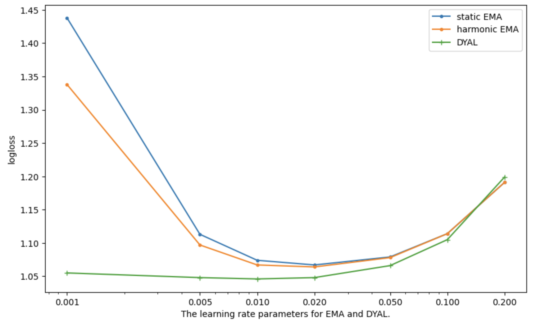
(a) new items, $O_{min}=50$

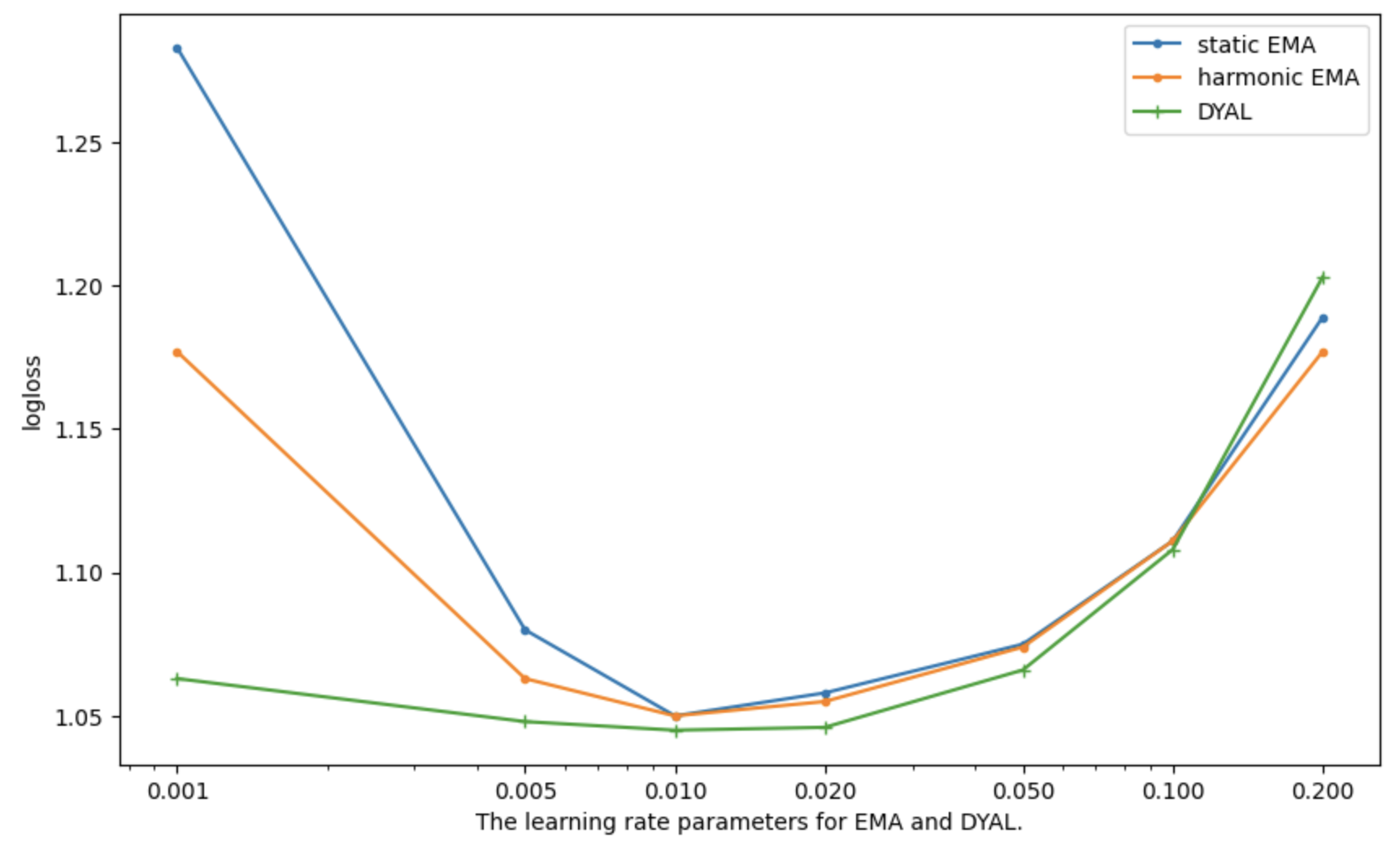
(b) recycle items, $O_{min}=50$

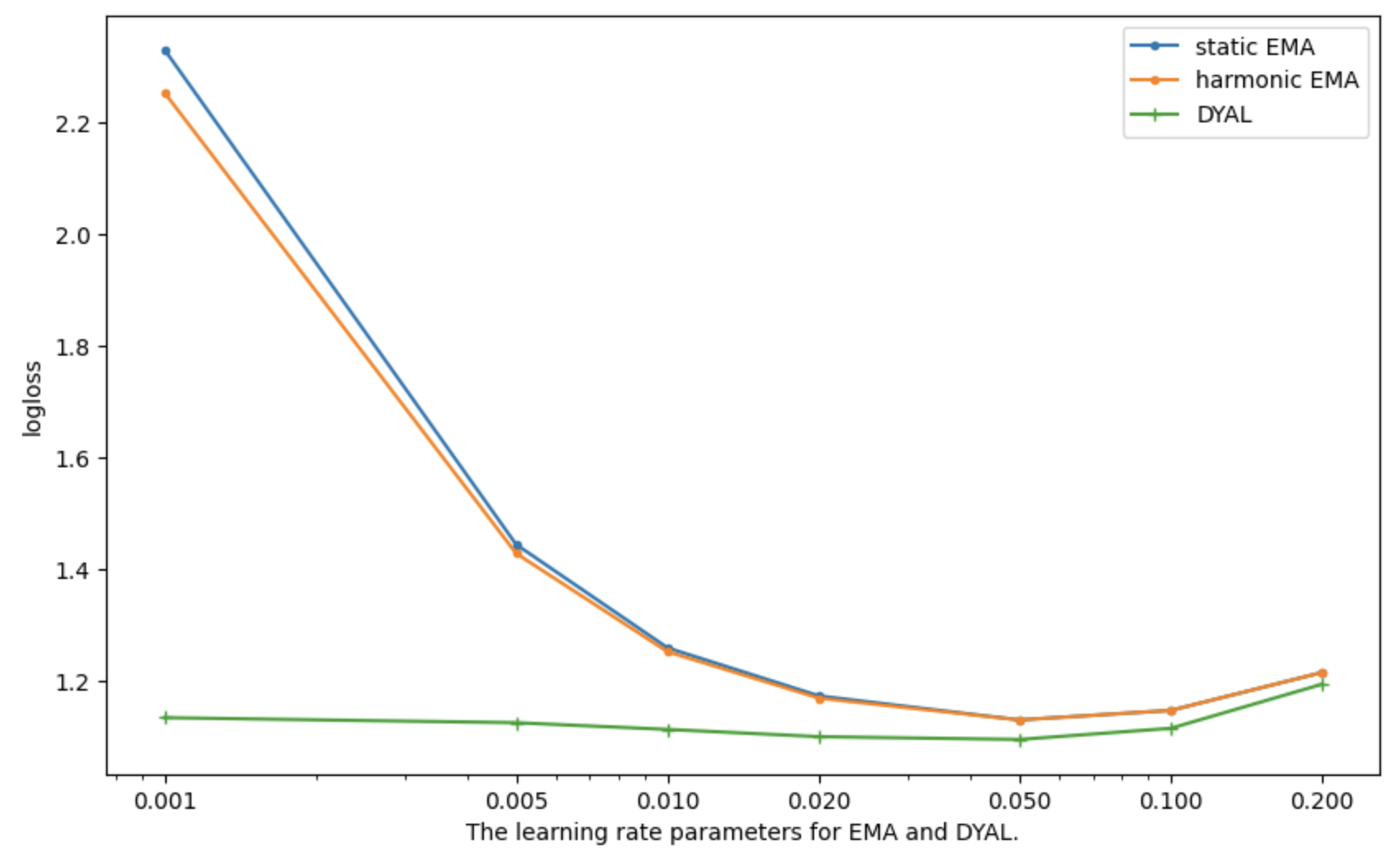
(c) new items, $O_{min}=10$

Figure 14: log-loss performance, as the learning rate is changed, in synthetic multi-item experiments, $O_{min}=50$. (a) new items. (b) recycle items. DYAL is less sensitive to how low $\beta_{min}$ is set, compared to harmonic and static EMA variants.

8 Experiments On Real-World Data Sources

In real-world datasets, a variety of complex phenomena combine to generate the sequences of observations, and even if we assume stationary distributions generate the data over some stable durations, we do not know the actual underlying probabilities in order to compare methods. In all the sections below, we obtain sequences of observations, in different domains, and report the log-loss performances, in particular AvgLogLossNS (Eq. 9), when comparing different predictors on these (same) sequences.

Table 7 presents the classification of the data sources we use here according to the type of non-stationarity. The sequences obtained from the Expedition system, an implementation of ideas in prediction games [26], and described next, exhibit what we have called internal or developmental non-stationarity: new items (concepts) are generated over time by the system itself. If we turn off concept generation and keep predicting at the character level in Expedition, we do not have any non-stationarity, with a static external text corpus and in the way we sample lines, and we report comparisons in this setting as well (Sect. 8.2), finding that DYAL, developed for non-stationarity, continues to enjoy performance advantages over the others in this setting too. We provide evidence that the sequences in our final task, the Unix commands data sequences (Sect. 8.3), exhibit external non-stationarity: each person’s pattern of command usage changes over days and months, as daily activities and projects change. An example of a task exhibiting both internal and external non-stationarity is feeding the Expedition system one genre or language (e.g. French) for some time, followed by another (e.g. Spanish). We leave experiments on tasks exhibiting both internal and external non-stationarity to the future.

8.1 Expedition: Up to N-Grams

The Expedition system operates by repeatedly inputing a line of text (on average, about 50 characters in these experiments), interpreting it, and learning from the final selected interpretation. The interpretation process consists of search and matching (Fig. 15): it begins at the low level of characters, which we call primitive concepts, and ends in the highest-level concepts in its current concept vocabulary $V$ that both match the input well and fit with one another well. Initially, this vocabulary $V$ corresponds to the set of characters, around 100 unique such in our experiments, but over many episodes the vocabulary with which the system interprets grows to thousands of concepts and beyond. In our experiments, concepts are n-grams (words and words fragments). Higher level n-grams help predict the data stream better, in the sense that bigger chunks of the stream (better predictands) can be predicted in one shot and fewer independence assumptions are made. In the Expedition system, concepts are both the predictors and the predictands.

8.1.1 An Overview of Simplified Expedition

Non-Stationarity $\rightarrow$	Internal	External
Expedition, up to n-grams	✓	–
Expedition, only characters	–	–
Unix commands	$-$	✓

Number	Median	Minimum	Maximum
104	1.2k	75	48k
Examples of recorded predictors, and sequence lengths:
(“ht”, 91), (“t s”, 75), (“and”, 144), (“ron”, 189),
(“th”, 3066), (“t”, 25k), (“ ”, 48k)

Table 7: Left: Real datasets and types of non-stationarity exhibited in the experiments. Right: Statistics on 104 Expedition sequences, with median sequence size of 1.2k. Blank space is the most frequent character leading to a sequence length of 48k, and ’t’ is the next most common at 25k.

In previous work, we developed and motivated an information theoretic concept quality score we named CORE. CORE is a measure of information gain, a reward or score that promotes discovering and use, within interpretations, of larger or higher-level (higher reward) concepts [28]. In this work, we ignore the quality of the concepts (the predictands), and focus only on the more “pure” prediction task of better predicting a sequence of (unit-reward) items in the face of non-stationarity. We also leave it to future work to carefully assess the impact of better prediction algorithms on the learning and development of the entire system, i.e. the performance of the overall system with multiple interacting parts. Here and in Appendix E, we briefly describe how a simplified Expedition system works, and how we extract sequences, for learning and prediction. There are three main tasks in Expedition:

1. Interpreting (in every episode): using current concept vocabulary $V$, segment a line of text (the episode input) and map the segments into highest-level concepts, creating a concept sequence.

2. Predicting and updating (learning) prediction weights (every episode): Using a final selected interpretation $s$, update prediction weights among concepts in interpretation $s$.

3. Composing (every so often): Make new concepts out of existing ones in $V$ (expand $V$).

In this paper, we focus on the prediction task 2, and to simplify the comparison of different prediction algorithms, we divorce prediction from interpreting and composing, so that the trajectory the system takes, in learning and using concepts, is independent of the predictor (the learner of the prediction weights), and different predictors can be directly compared. Otherwise, one needs to justify the intricacies of interpretation and new concept generation and that such do not unfairly work well with one technique over another. The interpretation and composing methods we used, for tasks 1 and 3, are described in Appendix E.

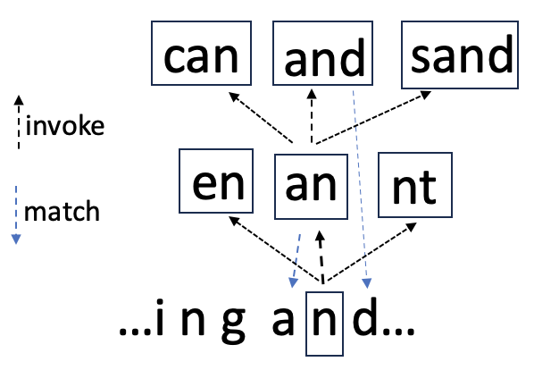
(a) Bottom to top interpretation (search) paths: invoking compositions (upward) and matching attempts (downward), in finding an interpretation.

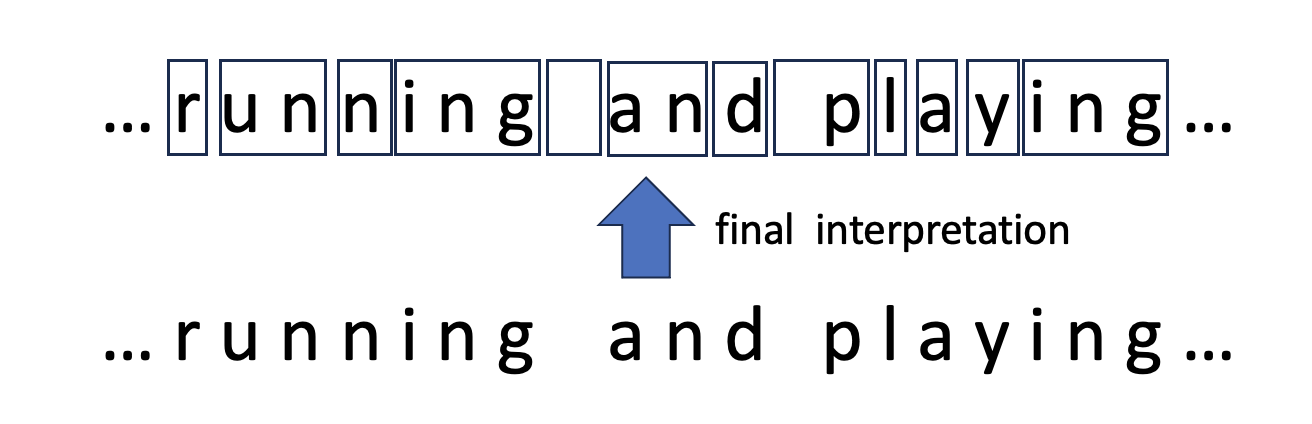
(b) An example final interpretation, given the input fragment "running and playing".

Figure 15: (a) The interpretation search process consists of invoking (“upward”) and matching attempts (“downward”), until no more compositions that match the input remain. (b) The final selected interpretation is a sequence of highest level available concepts, n-grams, that match the given input line well.

8.1.2 Prediction Tasks, and Collecting Sequences

In every episode, once an interpretation, i.e. a final concept sequence, is selected, each concept in the sequence, except the right most, acts as a predictor and updates its weight for predicting what comes immediately after it to the right. For example, in the concept sequence of Fig. 15(b), the predictor (concept) ’r’ observes the (concept) ’un’ to its right and updates accordingly, and (the predictor) ’un’ observes ’n’ to its right and updates accordingly, and so on. Note that only the final selected interpretation is used for updating prediction weights here, and the interpretation search path leading to it, as well as other search paths leading to unselected final interpretations, are discarded.

We ran the Expedition system for four trials, in each trial starting from scratch and with a different random seed, i.e. different sequences of lines are input to the system. Each trial lasted from 20k to 30k episodes, and in the course of a trial thousands of new concepts are generated and used. Id generation for concepts is incremental via a simple counter, and as characters are seen first, before any higher-level n-gram is generated, concepts with lower ids correspond to characters (unigrams) and after id 95 we get bigrams and trigrams.

In each trial, for each of a few arbitrary concept ids being tracked (a few below id 20, a few around 100 and 500), we collect and create a sequence from what comes after the corresponding concept in the episodes it is active in, i.e. it appears in one or more places in the final selected interpretation. For instance, in one trial, the concept (corresponding to) ’t’ was tracked, and ’t’ got a sequence of 25k observations long, each observation being a concept id. Thus ’t’ was active in up to 25k episodes (in some episodes, ’t’ may appear more than once). Initially, in the first few 100s of episodes say, ’t’ will only ’see’ single characters (unigrams) immediately next to its right (concept ids below 95), and later on, as bigrams and higher n-grams are generated, a mix of unigrams with higher level n-grams is observed. With tracking of a few ids, we collected 104 sequences over the different trials, with median sequence size of 1.2k observations, minimum size of 75, and maximum sequence size of 48k (Table 7). For the less frequent and newer concepts we get shorter sequences. There are nearly 1000 unique concepts (concept ids) in the longest sequences, and 10s of unique concepts in the shorter ones. A few example concepts with their sequence lengths are given in Table 7.

8.1.3 Internal Non-Stationarity in Expedition

Initially, every character (as a predictor) sees single characters in its stream of observations. For instance the character ’b’, as a predictor, sees ’a’, ’e’, ’ ’, etc. immediately occurring afterwards, for some time. Later on, as the higher level concepts, bigrams and trigram, are generated and used in interpretations, the predictor ’b’ also sees bigrams and trigrams (new concepts) in its input stream. Furthermore, when concept ’b’ joins another concept, such as ’e’, to create a new concept ’be’, the distribution around ’b’ changes too, as ’e’ is not seen to follow ’b’ as much as before the creation and use of ’be’: a fraction of the time when ’b’ occurs in an episode at the lowest level, now ’be’ is observed, at the highest level of interpretation, instead of the unigram ’b’ followed by ’e’. We also note that the frequency of the occurrence of a lower-level concept, at the highest interpretation level, tends to decrease over time as higher n-grams, that use that concept as a part, are generated and used.

The input corpus of text as well as the manner in which a text line is sampled (uniformly at random) to generate an episode is not changing here, i.e. no change in the occurrence statistics of individual characters, or there is no external non-stationarity here, but there is internal non-stationarity, as the interpretations tend to use highest level matching n-grams. Thus, the nature of the prediction task, at the highest interpretation level, can change gradually, even when the external input stream is stationary.

8.1.4 Overall Performance on 104 Expedition Sequences

Table 8 shows the log-loss (AvgLogLossNS()) scores of our 4 predictors, averaged over the 104 Expedition sequences. All the parameters are at their default when not specified, thus DYAL is run with binomial threshold of 5 and a queue capacity of 3. We observe that DYAL does best on average, and as Table 9 shows, pairing and performing sign tests indicates that log-loss of DYAL (with $\beta_{min}=0.001$) outperforms others over the great majority of the sequences.

Table 9 also changes the $c_{NS}$ to assess sensitivity to what is considered noise. Lowering the $c_{NS}$ makes the problem harder, and we have observed here and in other settings, that log-loss goes up. For instance, the log-loss performance of DYAL goes from $2.93$ at $c_{NS}=0$ down to $2.3$ with $c_{NS}=3$. Of course, with $c_{NS}=1$, we are expecting a technique to provide a good PR estimate even though the item has occurred only once before! Without extra information or assumptions, such as making the stationarity assumption and assuming that there are no noise items, or using global statistics on similar situations (e.g. past items that were seen once), this appears impossible.

We next go over the sensitivity and behavior of different techniques under parameter changes, as well as looking at performance on long vs. short sequences (subsets of the 104 sequences).

	Qs, 2	Qs, 3	Qs, 5	Qs, 10	Static, 0.001	Static, 0.01	Harmonic, 0.01	DYAL , 0.001
logloss	2.65	2.60	2.61	2.70	2.80	2.56	2.71	2.39

Table 8: log-loss of various methods on 104 sequences extracted from Expedition (median sequence size of 1.2k).

DYAL, 0.001 vs. $\rightarrow$	Qs, 3	static, 0.01	static, 0.005	harmonic, 0.01
$c_{NS}=3$	1, 103	0, 104	17, 87	0, 104
$c_{NS}=2$ (default)	1, 103	0, 104	16, 88	0, 104
$c_{NS}=1$	13, 91	22, 82	13, 91	8, 96
$c_{NS}=0$	17, 87	13, 91	2, 102	27, 77

Table 9: Number of losses and wins of DYAL, with $\beta_{min}=0.001$, pairing it against a few other techniques, on the 104 Expedition sequences, as we alter the $c_{NS}$ threshold. If observation count $\leq c_{NS}$ then it is marked NS (Sect. 3.6). Thus DYAL wins over Qs with (qcap $=3$) on 103 of 104 sequences (top left). The number of wins of DYAL is significant at over 99.9% confidence level in all cases. Also, DYAL wins over static with $\beta\in\{0.01,0.005\}$, on all the 19 longest sequences, at default $c_{NS}=2$.

8.1.5 Sensitivity to Parameters

Fig. 16(a) shows the sensitivity to $\beta_{min}$ for DYAL and harmonic EMA, and $\beta$ for static EMA. We observe, as in Sect. 7.3 for the case of multi-item synthetic experiments, that DYAL is less sensitive than both of harmonic and static EMA, while harmonic is less sensitive than static when $\beta$ is set low (and otherwise, similar performance to static). In particular, for longer sequences, lower rates can be better (see next Section), but for plain EMA variants, low rates remain an issue when faced with non-stationarity (i.e. new salient items).

Fig. 16(b) shows the sensitivity of DYAL to the choice of the binomial threshold, which controls when DYAL uses the queue estimates. There is some sensitivity, but we posit that at 3 and 5, DYAL performs relatively well. We also ran DYAL using different queue capacities with $\beta_{min}=0.001$ (default is $qcap=3$), and obtained similar log-loss results (e.g. $2.38$ at $qcap=2$, and $2.4$ for $qcap=5$).

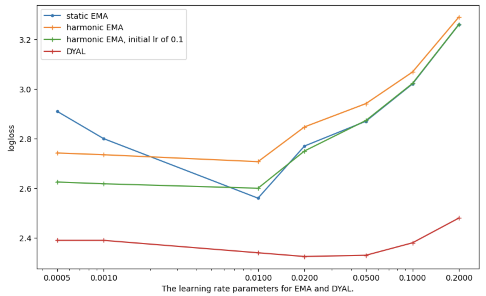
(a) Logloss vs learning rate.

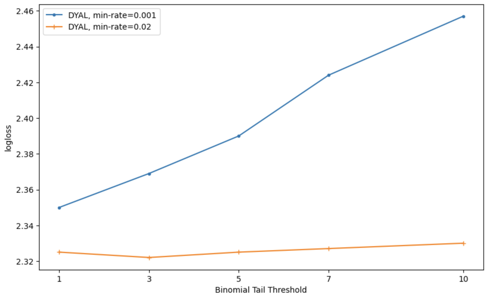
(b) Logloss vs binomial threshold, DYAL.

Figure 16: Prediction sequences from Expedition: Changing the learning rate (left), and the binomial threshold (right) in DYAL, and plotting the log-loss (AvgLogLossNS ()) performance.

8.1.6 Longer vs. Shorter Sequences

Of the 104 sequences, there are 19 sequences with length above 5k, median length being 13k. We averaged the log-loss performances of DYAL, as we change its $\beta_{min}$, over these 19, as well as over the sequences with length below 1k, of which there are 46 such, with median of 280 observations. Fig. 17(a) shows that lowering the $\beta_{min}$ works better or no worse, for longer sequences, as expected, while the best performance for the shorter sequences occurs with higher $\beta_{min}>0.01$. A similar patterns is also seen in Fig. 17(a) for Qs technique. Larger queue capacities work better for longer sequences, but because shorter sequences dominate the 104 sequences, overall we get the result that a qcap of 3 works best for this data overall.

We also note that the shorter sequences yield a lower log-loss (both figures of 17). This is expected and is due to our policy for handling NS: for methods that allocate most their initial mass to noise and when this agrees with the NS marker referee, one gets low loss. For instance, at $t=1$, the NS marker marks the next item as NS, and with a predictor that has all its PR mass unallocated, log-loss is 0 (loglossRuleNS() in Fig. 3(c)). As the sequence grows longer, and more salient items are discovered, the average loss can go up. This is also observed in the next section when we do character-based prediction.

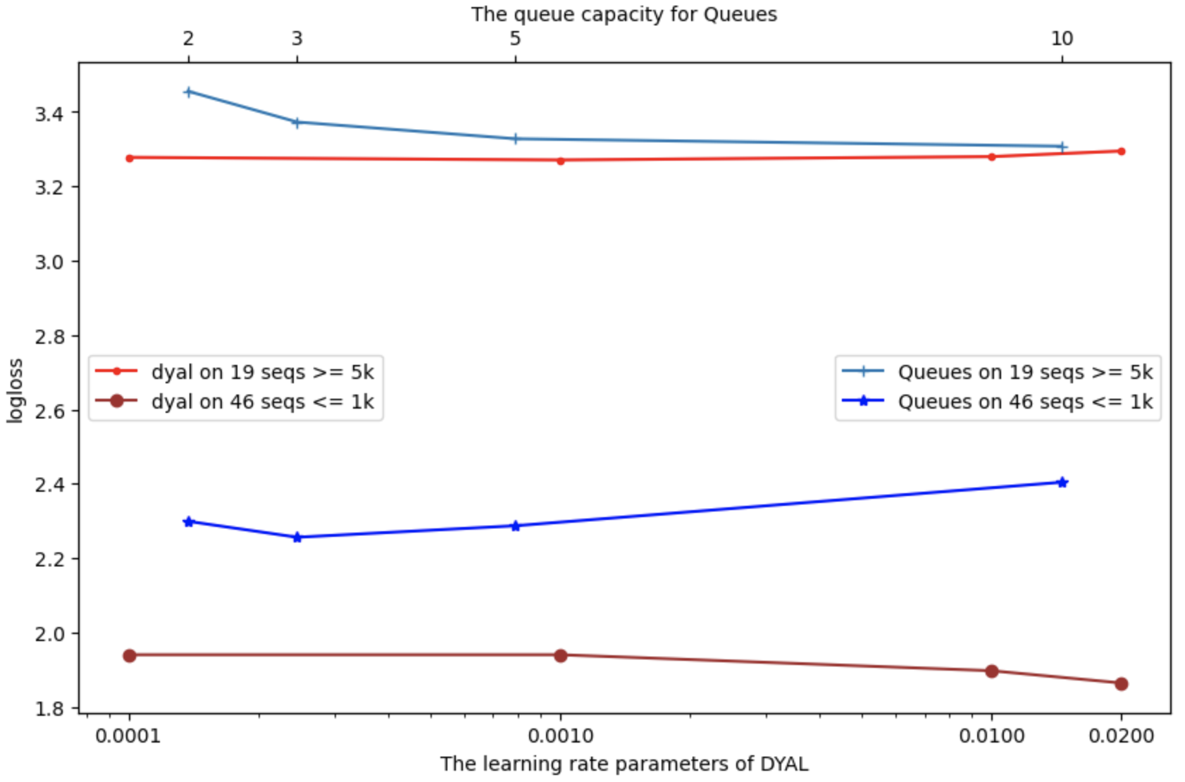
(a) Loss on longer vs. shorter sequences (DYAL and Qs).

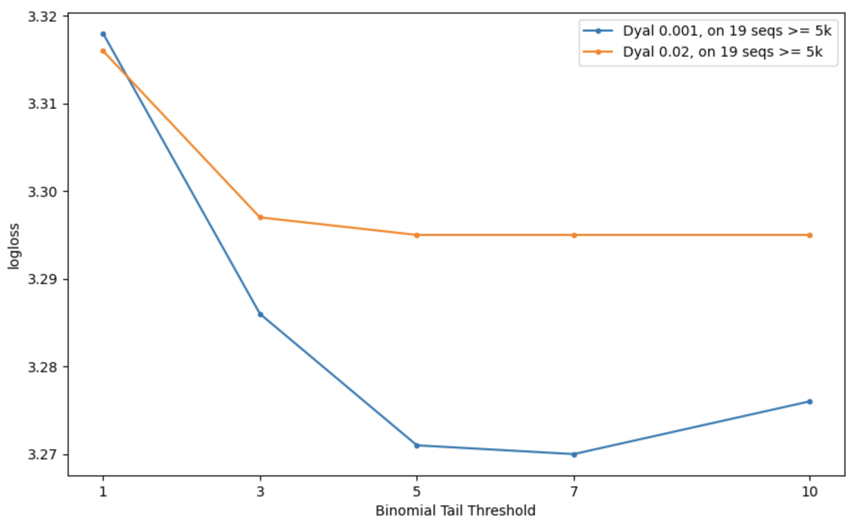
(b) Loss on 19 longest sequences vs. binomial threshold.

Figure 17: log-loss (a) on 19 longest sequences (above 5k) vs 46 shorter sequences (below 1000). On the longer sequences and lower $\beta_{min}$ for DYAL, and a higher queue capacity for Qs, helps. (b) loss vs binomial threshold on 19 longest sequences. Setting the value in 3 to 7 works well, and $\beta_{min}=0.001$ does better than $\beta_{min}=0.02$ on these sequences.

8.1.7 Evolution of the Learning Rates, Degrees, etc.

Fig. 18 shows plots of the evolution of maximum (max-rate) and median of the learning rates in the $rateMap$  of DYAL for two predictors (two sequences), the concept "ten", with just over 200 episodes, and the concept “l” with over 12000 episodes. The number of entries in the $rateMap$  (and the $EmaMap$), or the out-degree, is also reported. We observe that the maximum over the learning rates contain bursts every so often indicating new concepts need to be learned, while the median rate converges to the minimum, indicating that most predictands at any given time are in a stable state. On the long 12k sequence, we also see the effect of pruning the map every so often: the number of map entries remain below 100 as old and low PR items are pruned (see Sect. 5.6 and 6.3).

Appendix E.4 also includes plots of the max-rate on a few additional sequences (self-concatenations), in exploring evidence for non-stationarity.

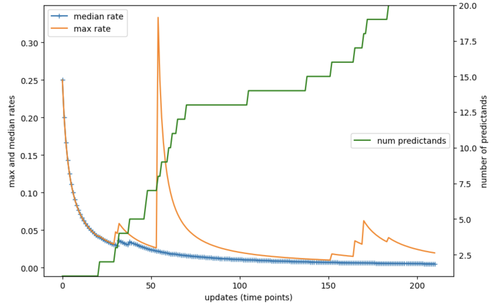
(a) Learning rates, max and median, and out-degree, for concept ’ten’ (via DYAL).

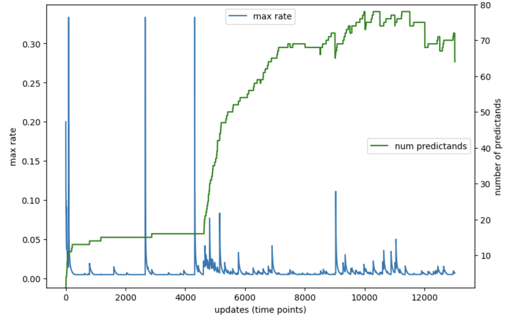
(b) Max rate and out-degree for ’l’.

Figure 18: Examples of evolution of the learning rates of DYAL and the number of predictands, or out-degree (number of entries in $EmaMap$), with time. (a) Maximum (max-rate) and median learning rates and number of predictands for the concept ’ten’. (b) Maximum learning rates and number of predictands for the 13k-long sequence for the concept ’l’.

8.2 Expedition at the Character level

Here, we do not generate new concepts, thus the prediction task remains at the (primitive) character level. We track all the characters as predictors: each character, when observed, predicts the next character, and, for evaluation, each has its own referee (NS marker). We report log-loss (AvgLogLossNS()) at every time point, meaning that with each input line, from left to right as in the previous section, for each character (predictor), we predict (what character comes to the right) and record the log-loss , then observe and update the predictor. At certain times $t$, e.g. after observing 1k characters (1000 observe and update events), we report the average of the log-losses upto $t$. For instance, on the line “abcd”, we collect the log-loss performance of the predictors corresponding to ’a’, ’b’ and ’c’ (and after the loss is collected, each predictor updates too). Thus, in this section, unlike the previous sections, we are reporting an average of the log-loss performance of different predictors, over time. Note further that, in this manner of reporting, the more frequent characters (predictors), such as ’e’, ’a’, and the blank space ’ ’, will have more of an impact on the reported performance.

In this character-prediction setting, there is neither external nor internal non-stationarity, as described in the previous section, and even though there is no non-stationarity, we find that DYAL out-performs the other predictors, as seen in Table 10 and Fig. 19. Table 10 shows log-loss averaged over 10 runs for a few choices of parameters, where a run went to 1k, 2k and 10k time points (prediction episodes). Fig. 19 shows log-loss performance for a few learning rates, from 10k to 300k time points. We see that DYAL with one choice of $\beta_{min}=0.001$, does best over all snapshots. The Qs technique does best with the highest capacity of 10 (in this stationary setting), and EMA variants require playing with the learning rate as before, and still lag DYAL. Plain EMA variants, static and harmonic, underperform for a combination of the way we evaluate and their insufficient inflexibility with regards to the learning rate: when an item is seen for the first time, harmonic may give it a high learning rate, but then is punished in subsequent time points, as the item may be a low probability event. Note that in our experiments, we started the harmonic with a initial learning rate of 1.0 (and experimenting with the choice of initial rate $\beta_{max}$ may improve its performance, see Fig. 20 on Unix commands). Static EMA assigns whatever its fixed learning rate is, to a new item, which could be too low or too high.

8.2.1 log-loss Initially Goes Up

Consistent with our previous observation on lower (better) log-loss performance on shorter vs. longer sequences (Sect. 8.1.6), here, as more seen items become salient (not marked NS), and with the manner we evaluate with a referee, log-loss increases over time for most methods but approaches a plateau and converges. For a ’slow’ method such as static EMA with a low $\beta$, log-loss peaks before it starts going down. DYAL is not slowed down or is not as sensitive to setting the (minimum) rate low ($\beta_{min}$ set to 0.001 or lower) (in Fig. 19, the plots for DYAL with $\beta_{min}$ from 0.0001 to 0.01 appear identical), and may actually benefit from a low rate in the long run (Table 11).

	Qs, 3	Qs, 5	Qs, 10	Static, 0.005	Static, 0.01	Static, 0.02	Harmonic, 0.01	DYAL, 0.001
1000	1.69$\pm$0.05	1.66	1.64	1.6	1.87	2.24	2.59	1.20
2000	2.01$\pm$0.02	1.96	1.93	2.11	2.16	2.34	2.50	1.60
10000	2.39$\pm$0.01	2.32	2.27	2.43	2.37	2.41	2.44	2.15

Table 10: log-loss averaged over 10 runs of character-level Expedition (no new concepts generated). DYAL does best over several time snapshots.

.

$\beta_{min}$ $\rightarrow$	0.0001	0.001	0.01	0.05	0.1
log-loss	2.408$\pm$0.002	2.398$\pm$0.001	2.415$\pm$0.000	2.512$\pm$0.002	2.652$\pm$0.001

Table 11: Character-level Expedition using DYAL over longer runs: log-loss averaged over 5 runs till 300k time points (character predictions). $\beta_{min}$ of $\geq 0.05$ is too high (indicating there are salient predictands with probability below $0.1$), while low $\beta_{min}\leq 0.001$ do slightly better than $0.01$.

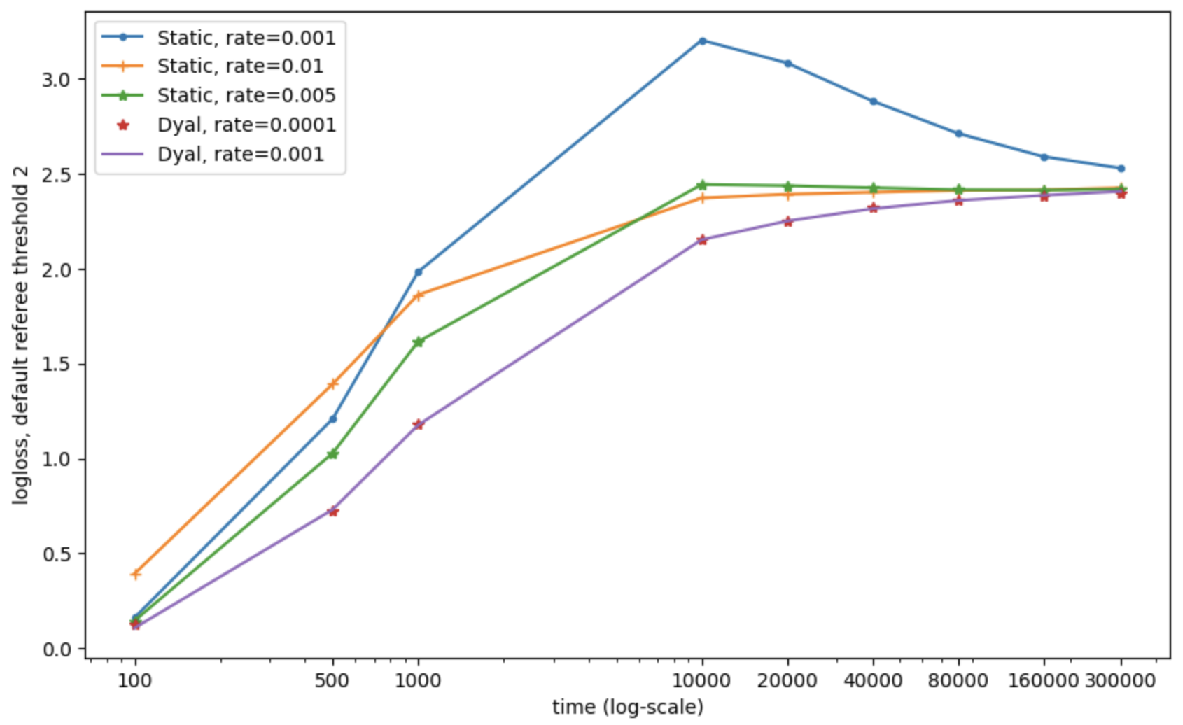
(a) Expedition at the character level (default $c_{NS}=2$).

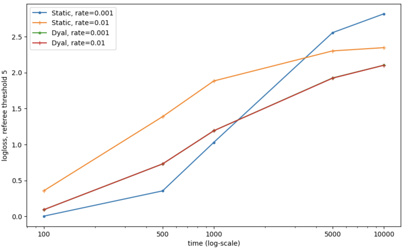
(b) Expedition at the character level, with relaxed $c_{NS}=5$.

Figure 19: log-loss vs time, for Expedition at the character level. (a) With default $c_{NS}=2$, each point is average over 5 sequences. (b) With the more relaxed $c_{NS}=5$ (shown up to 10000) initially all curves improve, lowered log-loss, compared to $c_{NS}=2$. In particular static EMA with a low rate benefits most, as it only slowly allocates probability to salient items, agreeing more with the relaxed referee. In both cases, DYAL with two different rates ($\beta_{min}\in\{0.0001,0.001\}$ in (a) and $\beta_{min}\in\{0.001,0.01\}$ in (b)) results in almost identical losses.

8.3 Unix Commands Data

52-scientists (52 sequences)
sequence length			# unique commands per user
median	min	max	median	min	max
1.8k	205	12k	106	22	359

Masqurade (50 sequences, 5k each)
# unique commands per user
median	min	max
101	5	138

Table 12: Statistics on Unix commands data. Left: 52-scientists, median sequence length is 1.8k commands, and the median number of unique commands per sequence is 106, while one user (sequence) has 138 unique commands (the maximum). Right: Masqurade, 50 sequences, each 5k long. Median number of unique commands per sequence is 101, while one user used only 5 unique commands (in 5k commands).

We look at two sequence datasets in the domain of user-entered Unix commands, which we refer to as the 52-scientists data, a subset of data collected by Greenberg [18], and the Masqurade sequences [41]. These sequences are good examples of high external non-stationarity: for instance, it is observed in our previous work on Greenberg sequences [29] that if the online updates are turned off mid-way during learning, when it appears that the accuracy has plateaued, the prediction performance steadily declines. We also present further evidence of non-stationarity below, as well as in Appendix E.4. The data likely includes a mix of other non-iid phenomena as streaks (repeating commands) and certain hidden periodic behaviors. Table 12 gives sequence statistics for the two sources.

8.3.1 Task and Data Description

In our previous work [29], we were interested in the ranking performance, for a recommendation or personalization task, and we used several features of context, derived from previously typed commands, as predictors of the next command. We learned and aggregated the predictions of the features using a variation of EMA that included mistake-driven or margin-based updates, and showed significant performance advantage over techniques such as SVMs and maximum entropy [29]. Here, we are interested in the extent to which the sequences are stable enough to learn probabilities (PRs), and the relative performance of different probabilistic prediction techniques. As the sequences would be relatively short if we focused on individual commands as predictors (100s long for almost all cases), we look at the performance of the “always-active” predictor that tries to learn and predict a “moving prior” of which next command is typed. Therefore here, each command in the sequence is an item. For both datasets, we use only the command stubs, i.e. Unix commands such as “ls”, “cat”, “more”, and so on, without their arguments (filenames, options, etc.). The Masqurade data has the stubs only, and our experiments with full commands, vs. stubs only, on 52-scientists yields similar observations. The sequences have been collected over the span of days to months for both datasets, depending on the level of the activity of a user. For Masqurade, we only use the first 5000 commands entered by each user, as the remainder can have other users’ commands interespersed, designed for the Masqurade detection task [41].

8.3.2 Performance on Unix Data

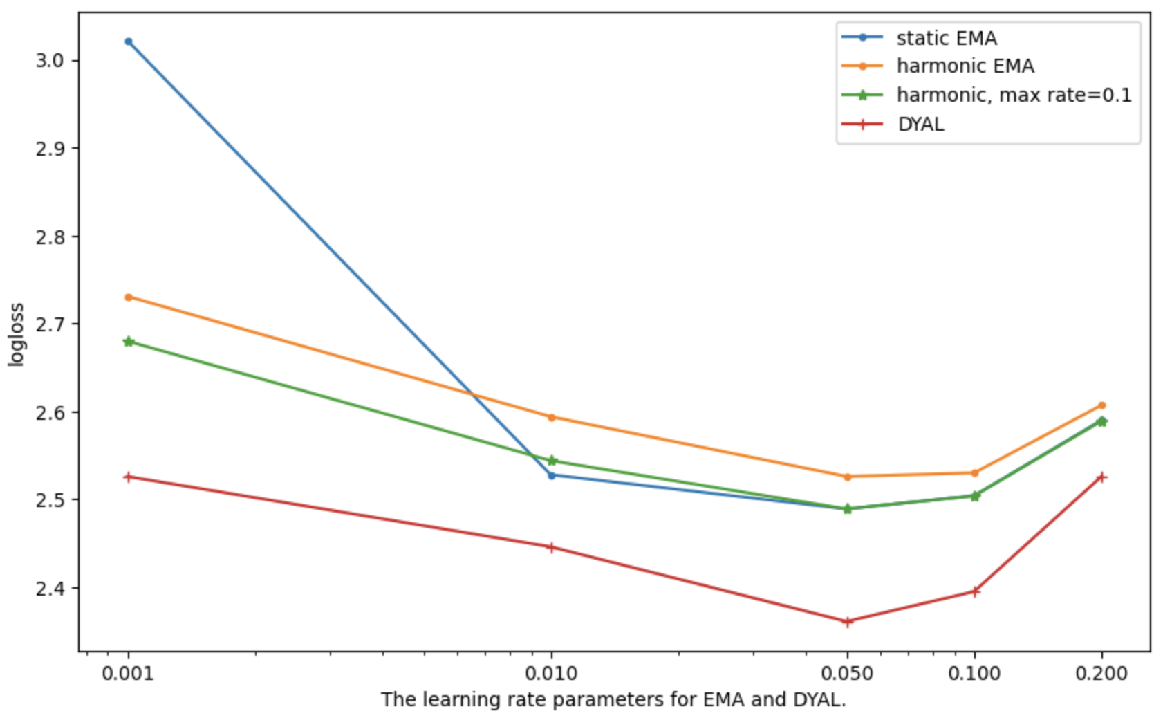
(a) log-loss vs rate, Unix 52-scientists sequences.

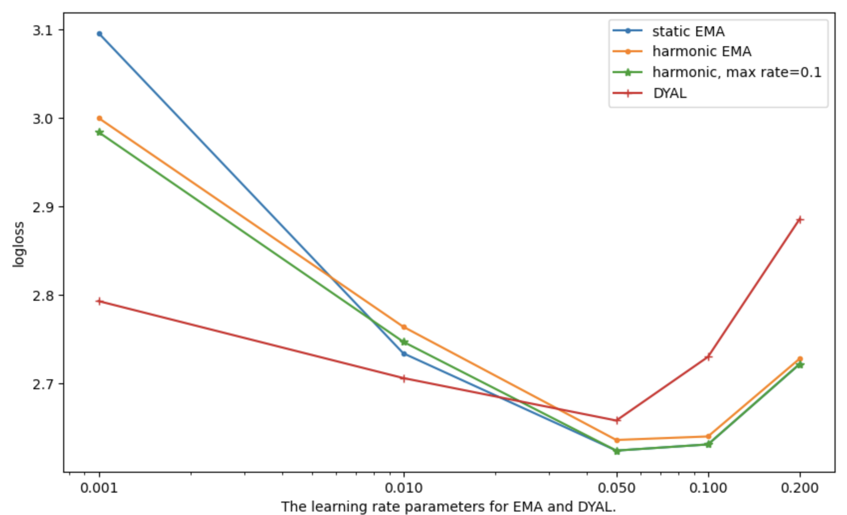
(b) log-loss vs rate, Unix Masqurade sequences.

Figure 20: log-loss performances (AvgLogLossNS()) vs. $\beta$ parameters: (a) 52-scientists (b) Masqurade.

Fig. 20 shows the performance of EMA variants as a function of the learning rate, and Table 13 reports on Qs performance with a few qcap values, and includes the best of EMA variants. We observe a similar v-shape pattern of performance for static and harmonic EMA, while for DYAL, as before, the plots show less of a dependence on $\beta_{min}$ compared to other EMA variants. However, the degradatation in performance as we lower $\beta_{min}$ is more noticeable here. DYAL performs better on 52-scientists compared to others, but is beaten by static EMA on Masqurade. Below, we report on paired comparisons and the effect of changing the referee threshold $c_{NS}$.

We note these data indeed have higher non-stationarity compared to previous ones when we consider a few indicators: the best performance occurs when $\beta_{min}$ is relatively high at $\approx 0.05$, larger than our previous datasets (Fig. 20). Table 13 also shows that Qs does best here with smaller qcap values. Appendix E.4 presents additional experiments showing further evidence of external non-stationarity.

52-Scientists					Masqurade
Qs, 2	Qs, 3	Qs, 5	Qs, 10	DYAL, 0.05	Qs, 2	Qs, 3	Qs, 5	Qs, 10	Static, 0.05
2.581$\pm$0.28	2.586	2.629	2.686	2.361	2.769$\pm$0.5	2.735	2.754	2.830	2.624

Table 13: On Unix sequences, Qs log-loss performance, and the best of EMA variants. Lower qcaps work better, suggesting significant non-stationarity.

8.3.3 Pairing and Sign-Tests on Unix Sequences

We compare DYAL to static EMA as harmonic and static behave similarly. At $\beta$ of 0.05, best for both DYAL and static EMA, on the 52-scientist sequences, we get 46 wins for DYAL over static (lower log-loss for DYAL), and 6 wins for static. On average, 13% of a sequence is marked NS. As we raise the referee threshold $c_{NS}$ from 2 to 3 to 4, we get additional wins for DYAL and the log-loss perfromances improve for all methods, and the fraction of sequence marked NS goes up, reaching to 18% at $c_{NS}=4$. Conversely if we lower the referee threshold to 1, we get fewer 34 wins for DYAL over static EMA (and 11% marked NS).

On Masqurade’s 50 sequences, we get only 10 wins for DYAL vs. 40 for static, again at $\beta_{min}=0.05$, where both do their best, which is statistically highly signifcant. With the default of $c_{NS}=2$ only 5% of a sequence is marked NS on average. As in the case of 52-scientists, when we increase the referee threshold from 2 to 3 to 4, we get additional wins for DYAL, and at $c_{NS}=4$, DYAL has 37 wins over 13 wins for static (8% marked NS with $c_{NS}=4$). Similarly lowering the threshold to 1 leads to more wins for static. Importantly, if use a referee that is based on a short window of the last 200 (rather than our simple unlimited window size) and require seeing an item at least twice in the last 200 timepoints to mark it as salient (not NS), again DYAL becomes superior (47 wins for DYAL, and 9% marked NS).

Why a fixed and relatively high learning rate of 0.05 does relatively well here compared to the more dynamic DYAL, on Masqurade sequences? Any assumption behind the design of DYAL, in particular the sufficient stability assumption, may be partially failing here. For many items, their PR, or appearance frequency, may be high once they appear, but their stability period may be too short, and a simple high learning-rate of 0.05 may work just as well, compared to the slow two-tiered approach of first detection and estimation via the Qs technique, and at some point, switching to the queues estimate. As we increase the referee threshold $c_{NS}$, we focus or bias the evaluation further on the more stable items in the sequence, and we get better relative results for DYAL. This observation gives more credence to the stability explanation.

9 Related Work

We provided pointers on relevant work for the tools and techniques we used throughout the paper. In this section, we briefly situate our work within the broader context of similar tasks and problem domains, and provide a short history.

This paper extends our ongoing work on developing large-scale online multiclass learning techniques, for lifelong continual learning when the set of classes is large and dynamic [30, 31], in particular in the framework of prediction games for learning a growing vocabulary of concepts [28, 25, 26]. In online (supervised) learning, e.g. [20, 39, 24], the focus is often on the interaction of the predictors (features) and, for example, on learning a good weighting combination for a linear model, while we have focused on learning good independent probabilistic predictors, akin to the (multiclass) Naive Bayes model [23], as well as the counting techniques for n-gram language models [40], but in a non-stationary setting. Investigating online techniques for learning good mixing weights, also handling the non-stationarities, may prove a fruitful future direction, for instance in the mold of (sleeping) experts algorithms [14, 20, 9].

Our task and solution involves a kind of change detection, and change detection is a diverse subject studied in several fields such as psychology (e.g. in human vision) and image processing and time series analysis [47, 4, 7]. Here, we also seek a response or an adaptation to the change. The online observe-update cycle of a semi-distribution has a resemblance to online (belief) state estimation, e.g. in Kalman filters and partially observed Markov models for control and decision making, in particular with a discrete state space [10, 7]. Here, the goal is pure prediction, though some of the techniques developed here may be relevant, specially when one faces a changing external world. Streaming algorithms aim to compute useful summary statistics, such as unique counts and averages, while being space and time efficient, in particular often requiring a single pass over a large data set or sequence, such as the count-min sketch algorithm [15]. Here, we have been interested in computing recent proportions in a non-stationary setting, for continual prediction, implemented by each of many (severely) resource-bounded predictors.

Learning rate decay has been shown beneficial for training on backpropagation-based neural networks, and there is research work at explaining the reasons [50, 44]. Here, we motivated decay variants in the context of EMA updates and learning good probabilities fast, and motivated keeping predictand-specific rates.

10 Summary and Future Directions

Dynamic worlds require dynamic learners. In the context of online multiclass probabilistic prediction, we presented three sparse moving average techniques for resource-bounded (finite-space) predictors. We described the challenges of assessing probability outputs and developed a method for evaluation, based on log-loss, under noise and non-stationarity. We showed that different methods work best for different levels of non-stationarity, but provided evidence that in the regime where the probabilities can change substantially but only after intermittent periods of stability, the DYAL technique which is a combination of the sparse EMA and the Qs technique, is more flexible and has advantages over either of the simpler methods: the Qs predictor has good sensitivity to abrupt changes (can adapt fast), but also has higher variance, while plain EMA is slower but is more stable, and combining the two leads to faster more robust convergence in the face of non-stationarities.

This work arose from the problem of assimilating new concepts (patterns), within the prediction games framework, where concepts serve as both the predictors and the predictands in the learning system. In particular, here we made a distinction that even if the external world is assumed stationary, the development of new concepts, explicitly represented in the system, results in internal, or developmental, non-stationarity, for the many learners within the system. This means sporadic abrupt changes in the co-occurrence probabilities among the concepts seen at the highest-level as the system changes and evolves its interpretation of the raw input stream. However, we expect that the rate of the generation of new concepts can be such that there would be stability periods, long enough to learn the new probabilities, both to predict well and to be predicted well. Still, we strive for predictors that are fast in adapting to such patterns of change.

We plan to further evaluate and develop the prediction techniques within the prediction games framework, in particular under longer time scales and as better concept generation and interpretation techniques are developed, and we seek to better understand the interaction of the various system components. We touched on a variety of directions in the course of the paper. For instance, it may be fruitful to take into account item (predictand) rewards when rewards are available (such as in prediction games), and this could lead to different and interesting design changes in the prediction algorithms, or how we evaluate.

Appendix A Further Material for the Evaluation Section

In this section, we provide proofs and further details for the evaluation section 3, in particular developing properties that indicate the near propriety of LogLossNS() in Sect. A.3, including extensions of KL() to SDs and how scaling and shifting SDs affects optimality of SDs under KL divergence. Sect. A.4 discusses a few alternatives that we considered for evaluating sequence prediction when using log-loss and handling noise (NS) items.

A.1 Quadratic Loss

Lemma.

(sensitivity of QuadLoss to the magnitude of PR shifts only) Given DI $\mathcal{P}$ and SD $Q$, defined over the same finite set $\mathcal{I}$,

            $\mbox{QuadLoss}(Q|\mathcal{P})=\mbox{QuadDist}(Q,\mathcal{P})$

Proof.

This property has been established when both are DIs (i.e. when $\mbox{sum}(Q)=1$) [42], and similarly can be established by writing the expectation expressions, rearranging terms, and simplifying. We give a proof by reducing to the DI case: when $Q$ is a strict SD, we can make a DI variant of $Q$, call it $Q^{\prime}$, via adding an extra element $j$ to $\mathcal{I}$ with remainder PR $Q^{\prime}(j)=1-\mbox{sum}(Q)$ (note: $\mathcal{P}(j)=0$). Observing the following 3 relations establishes the result: 1) $\mbox{QuadDist}(\mathcal{P},Q)=\mbox{QuadDist}(\mathcal{P},Q^{\prime})-Q^{\prime}(j)^{2}$, 2) $\mbox{QuadLoss}(Q^{\prime}|\mathcal{P})=\mbox{QuadDist}(Q^{\prime},\mathcal{P})$ (as both are DIs), and 3) $\mbox{QuadLoss}(Q^{\prime}|\mathcal{P})=\mbox{QuadLoss}(Q|\mathcal{P})+Q^{\prime}(j)^{2}$, as with every draw from $\mathcal{P}$ we incur the additional cost of $Q^{\prime}(j)^{2}$ compared to the cost from $Q$): by definition, we have, $\mbox{QuadLoss}(Q^{\prime}|\mathcal{P})=\sum_{i\in\mathcal{I},i\neq j}\mathcal{P}(i)\left(Q^{\prime}(j)^{2}+(1-\mathcal{P}(i))^{2}+\sum_{u\in\mathcal{I},u\neq i,u\neq j}\mathcal{P}(u)^{2}\right)=\sum_{i\in\mathcal{I},i\neq j}\mathcal{P}(i)Q^{\prime}(j)^{2}+\sum_{i\in\mathcal{I},i\neq j}\mathcal{P}(i)\left((1-\mathcal{P}(i))^{2}+\sum_{u\in\mathcal{I},u\neq i,u\neq j}\mathcal{P}(u)^{2}\right)=Q^{\prime}(j)^{2}+\mbox{QuadLoss}(Q|\mathcal{P})$ (the last equality in part follows from $\sum_{i\in\mathcal{I},i\neq j}\mathcal{P}(i)=1$). ∎

This corollary immediately follows.

Corollary 2.

(sensitivity of QuadLoss to the magnitude of PR shifts only) With DI $\mathcal{P}$ and SD $Q$ (on the same items $\mathcal{I}$), let $\Delta_{i}=\mathcal{P}(i)-Q(i)$. Then $\mbox{QuadLoss}(Q|\mathcal{P})=\sum_{i\in\mathcal{I}}\Delta_{i}^{2}$.

A.2 The Sensitivity of log-loss

A corollary to Lemma 2 on equivalence of log-loss with KL() (relative entropy), where, for this corollary on sensitivity, without loss of generality, we are using items (dimensions) 1 and 2:

Corollary.

(LogLoss is much more sensitive to relative changes in larger PRs) Let $\mathcal{P}$ be a DI over two or more items ($\mathcal{I}=\{1,2,\cdots\}$, $|\mathcal{I}|\geq 2$), with $\mathcal{P}(1)>\mathcal{P}(2)>0$, and let the multiple $m=\frac{\mathcal{P}(1)}{\mathcal{P}(2)}$ (thus $m>1$). Consider two SDs $Q_{1}$ and $Q_{2}$, with $Q_{1}$ differing with $\mathcal{P}$ on item 1 only ($\forall i\in I$ and $i\neq 1$, $Q(i)=\mathcal{P}(i)$), and assume moreover $\mathcal{P}(1)>Q_{1}(1)>0$, and let $m_{1}=\frac{\mathcal{P}(1)}{Q_{1}(1)}$ (thus, $m_{1}>1$). Similarly, assume $Q_{2}$ differs with $\mathcal{P}$ on item 2 only, and that $\mathcal{P}(2)>Q_{2}(2)>0$, and let $m_{2}=\frac{\mathcal{P}(2)}{Q_{2}(2)}$. We have $\mbox{LogLoss}(Q_{2}|\mathcal{P})<\mbox{LogLoss}(Q_{1}|\mathcal{P})$ for any $m_{2}<m_{1}^{m}$.

Proof.

We write the difference $\Delta$ in the losses and simplify: $\Delta=\mbox{LogLoss}(Q_{1}|\mathcal{P})-\mbox{LogLoss}(Q_{2}|\mathcal{P})=\mathcal{P}(1)\ln\frac{\mathcal{P}(1)}{Q_{1}(1)}-\mathcal{P}(2)\ln\frac{\mathcal{P}(2)}{Q_{2}(2)}$ (all other terms are 0, e.g. $Q_{1}(2)=\mathcal{P}(2)$, and the entropy terms cancel). We thus have $\Delta=m\mathcal{P}(2)\ln(m_{1})-\mathcal{P}(2)\ln(m_{2})$, or we have $\Delta>0$ as long as $\ln(m_{1}^{m})-\ln(m_{2})>0$, or whenever $m_{1}^{m}>m_{2}$. ∎

A.3 On the (Near) Propriety of LogLossNS()

In the iid generation setting based on SD $\mathcal{P}$, when using a perfect NS-marker and using FC() parameterized by $P_{NS}$ and $P_{min}$, $\mathcal{P}$ is optimal (scores lowest) for LogLossNS() in several cases detailed below, and otherwise, an optimal $Q\neq\mathcal{P}$ is close to $\mathcal{P}$ in a certain sense, when $P_{NS}$ and $P_{min}$ are small. At the end of this subsection, we discuss the case of an imperfect practical NS-marker briefly.

Below we show that LogLossNS() is equivalent to a KL() divergence, as in plain log-loss but the KL() is based on transformations of SDs (scaling and filtering, augmenting). In particular, first we define augmentation of an SD to a corresponding DI that has one extra item with all remaining PR mass. This allows us to draw from $\mathcal{P}$ (as if it were DI, in particular for the purpose of evaluating LogLossNS(): We show computing LogLossNS($Q|\mathcal{P}$) is equivalent to computing KL() on the augmented versions, of $\mathcal{P}$ and FC($Q$).

Definition 3.

Definitions of augmenting an SD to a DI, and KL divergence for SDs:

• Given a non-empty SD $\mathcal{P}$ defined on $\mathcal{I}=\{1,\cdots,k\},k\geq 1$, its augmentation (operation), denoted $\mbox{DI}(\mathcal{P})$, is a corresponding DI $\mathcal{P}^{\prime}$, where $\mathcal{P}^{\prime}$ is defined on $\mathcal{I}^{\prime}$, $\mathcal{I}^{\prime}=\mathcal{I}\cup\{0\}$, $\mathcal{P}^{\prime}(0)=1-\mbox{sum}(\mathcal{P})$, and $\mathcal{P}^{\prime}(i)=\mathcal{P}(i)$, $\forall i\in I$.

• $\mbox{KL}_{NS}(\mathcal{P}||Q):=\mbox{KL}(\mbox{DI}(\mathcal{P})||\mbox{DI}({\bf FC}(Q)))$

For a DI $\mathcal{P}$, $\mbox{DI}(P)=\mathcal{P}$ in the sense that all positive PRs match, and for two SDs $\mathcal{P}$ and $Q$, $\mathcal{P}\neq Q\Leftrightarrow\mbox{DI}(\mathcal{P})\neq\mbox{DI}(Q)$. Unlike $\mbox{KL}()$, we note that $\mbox{KL}_{NS}(\mathcal{P}||\mathcal{P})$ can be positive, as ${\bf FC}()$ used on the 2nd parameter of $\mbox{KL}_{NS}$, here $\mathcal{P}$, can alter it, i.e. can filter and scale it, while $\mathcal{P}$ provided as first parameter is only augmented. We also note that there is another distinct way of obtaining a DI from a strict SD $\mathcal{P}$, that of scaling it, to $\alpha\mathcal{P}$, where $\alpha=\frac{1}{\mbox{sum}(\mathcal{P})}$. Both operations are useful, and used below.

Lemma 5.

For any two SDs $\mathcal{P}$ and $Q$ defined on $\mathcal{I}=\{1,\cdots,k\}$, where $\mathcal{P}$ is non-nempty, and using a perfect NS-marker wrt to $\mathcal{P}$:

$$\mbox{\bf LogLossNS}(Q|\mathcal{P})=\mbox{Entropy}(\mbox{DI}(\mathcal{P}))+\mbox{KL}_{NS}(\mathcal{P}||Q).$$

Proof.

We first explain the different parts of $\mbox{\bf LogLossNS}(Q|\mathcal{P})$, i.e. ${\mathbb{E}_{o\sim\mathcal{P}}}(\mbox{{\bf loglossRuleNS}}(o,Q,isNS(o)))$, to show that it is equivalent to comparing two augmented DIs under KL().

Let $Q^{\prime}={\bf FC}(Q)$ and $\mathcal{P}^{\prime}=\mbox{DI}(\mathcal{P})$. An item $o\sim\mathcal{P}$ (drawn from $\mathcal{P}$), is salient with probability $\mbox{sum}(\mathcal{P})$ ($o\in\sup(\mathcal{P})$), and otherwise is an NS item and is marked NS, the NS-marker being perfect, and it is important to note that $o$ does not occur in $\mathcal{I}$ ($Q^{\prime}(o)=Q(o)=\mathcal{P}(o)=0$ when $o$ is marked NS), with our uniqueness assumption when generating NS items. When we use loglossRuleNS(), the score in the NS case is $-\ln(1-\mbox{sum}(Q^{\prime}))$. This case occurs $1-\mbox{sum}(\mathcal{P})$ of the time, and a salient item $i$, $i\in\mathcal{I}$, occurs $\mathcal{P}(i)$ of the time, thus $\mbox{\bf LogLossNS}(Q|\mathcal{P})=-(1-\mbox{sum}(\mathcal{P}))\ln(1-\mbox{sum}(Q^{\prime}))-\sum_{i\in I}\mathcal{P}(i)\ln(Q(i))$, and adding and subtracting $\mbox{Entropy}(\mathcal{P}^{\prime})$ establishes the equivalence (where, $\mbox{Entropy}(\mathcal{P}^{\prime})=-(1-\mbox{sum}(\mathcal{P}))\ln(1-\mbox{sum}(\mathcal{P}))-\sum_{i\in I}\mathcal{P}(i)\ln(P(i))$):

$$\mbox{\bf LogLossNS}(Q|\mathcal{P}) =-(1-\mbox{sum}(\mathcal{P}))\ln(1-\mbox{sum}(Q^{\prime}))-\sum_{i\in I}\mathcal{P}(i)\ln(Q^{\prime}(i))-\mbox{Entropy}(\mathcal{P}^{\prime})+\mbox{Entropy}(\mathcal{P}^{\prime})$$

$$=(1-\mbox{sum}(\mathcal{P}))\ln\frac{1-\mbox{sum}(\mathcal{P})}{1-\mbox{sum}(Q^{\prime})}+\sum_{i\in I}\mathcal{P}(i)\ln\frac{\mathcal{P}(i)}{Q^{\prime}(i)}+\mbox{Entropy}(\mathcal{P}^{\prime})$$

$$=\mbox{KL}(\mathcal{P}^{\prime}||\mbox{DI}(Q^{\prime}))+\mbox{Entropy}(\mathcal{P}^{\prime})=\mbox{KL}_{NS}(\mathcal{P}||Q)+\mbox{Entropy}(\mbox{DI}(\mathcal{P}))$$

∎

The following (near) propriety properties follow as corollaries of Lemma 5:

Lemma.

Given a non-empty SD $\mathcal{P}$ generating sequences, using a perfect NS-marker, and using FC() to constrain candidate SDs, with $P_{NS}>0$ but assuming no PRs from $\mathcal{P}$ are dropped when applying FC() to $\mathcal{P}$ (e.g. $P_{min}=0$, or more generally $P_{min}<\min(\mathcal{P})$ even after possible scaling within FC()):

1. If $\mbox{sum}(\mathcal{P})\leq 1-P_{NS}$, then $\mathcal{P}$ is a minimizer of LogLossNS(), and it is the unique minimizer when $P_{min}=0$ and $\mbox{sum}(\mathcal{P})<1-P_{NS}$.

2. If $\mbox{sum}(\mathcal{P})>1-P_{NS}$, then $\mbox{KL}_{NS}(\mathcal{P}||\mathcal{P})\leq-\ln(1-P_{NS})$.

Proof.

We let $\mathcal{P}^{\prime}=\mbox{DI}(\mathcal{P})$, defined over $\mathcal{I}^{\prime}=\{0\}\cup\mathcal{I}$. Proof of claim 1: In this case, we note that ${\bf FC}(\mathcal{P})=\mathcal{P}$ (because $\mbox{sum}(\mathcal{P})\leq 1-P_{NS}$ and the assumption that no PRs are dropped from $\mathcal{P}$), (thus, $\mbox{DI}({\bf FC}(\mathcal{P}))=\mathcal{P}^{\prime}$), so setting $Q$ to $\mathcal{P}$ yields $\mbox{KL}(\mathcal{P}^{\prime}||\mbox{DI}({\bf FC}(\mathcal{P})))=\mbox{KL}(\mathcal{P}^{\prime}||\mathcal{P}^{\prime})=0$ (the minimum). It is the unique minimizer because when $P_{min}=0$ and $\mbox{sum}(\mathcal{P})<1-P_{NS}$, we can show that if $Q\neq\mathcal{P}$, ${\bf FC}(Q)\neq\mathcal{P}$, and thus we must have $\mbox{DI}({\bf FC}(Q))\neq\mathcal{P}^{\prime}$: first $Q$ must have an identical support set as $\mathcal{P}$, otherwise ${\bf FC}(Q)\neq\mathcal{P}$ ($P_{min}=0$ and scaling alone does not change the support set). Second (with the same support), if $\mbox{sum}(Q)<1-P_{NS}$, it is not altered by FC, therefore $Q^{\prime}=Q\neq\mathcal{P}$. Finally, if $\mbox{sum}(Q)\geq 1-P_{NS}$, we must have $\mbox{sum}({\bf FC}(Q))=1-P_{NS}\Rightarrow$ ${\bf FC}(Q)\neq\mathcal{P}$.

Proof of claim 2: Here $\mbox{sum}(\mathcal{P})>1-P_{NS}$, and for evaluating $\mbox{\bf LogLossNS}(\mathcal{P}|\mathcal{P})$, $\mathcal{P}$ is scaled in ${\bf FC}()$, i.e. FC($\mathcal{P}$)$=\alpha\mathcal{P}$, where $\alpha=\frac{1-P_{NS}}{\mbox{sum}(\mathcal{P})}$ (note: $1-P_{NS}\leq\alpha<1$), and $\mbox{\bf LogLossNS}(\mathcal{P}|\mathcal{P})=\mbox{KL}(\mathcal{P}^{\prime}||\mbox{DI}({\bf FC}(\mathcal{P})))=\sum_{i\in\mathcal{I}}\mathcal{P}(i)\ln\frac{\mathcal{P}(i)}{\alpha\mathcal{P}(i)}+(1-\mbox{sum}(\mathcal{P}))\ln\frac{1-\mbox{sum}(\mathcal{P})}{P_{NS}}\leq\sum_{i\in\mathcal{I}}\mathcal{P}(i)\ln\frac{\mathcal{P}(i)}{\alpha\mathcal{P}(i)}\leq-\ln\alpha\leq-\ln(1-P_{NS})$. ∎

We note that, for the first part above, when $\mbox{sum}(\mathcal{P})=1-P_{NS}$, then one can verify that for any $Q=\alpha\mathcal{P}$, where $\alpha\in[1,\frac{1}{1-P_{NS}}]$, $Q$ also minimizes $\mbox{\bf LogLossNS}(Q|\mathcal{P})$, as ${\bf FC}(Q)=\mathcal{P}$. However, the PR of no item in such $Q$ deviates more than $\alpha\leq\frac{1}{1-P_{NS}}$ (i.e. $\forall i,\frac{Q(i)}{\mathcal{P}(i)}\leq\frac{1}{1-P_{NS}})$, and with $P_{NS}$ small (e.g. $P_{NS}=0.01$), the deviations are therefore small. Similarly, for the second claim, we observe that $\mathcal{P}$ scores near optimal, i.e. has near 0 KL() divergence, for small $P_{NS}$ (no more than $-\ln(0.99)\approx 0.01$ when $P_{NS}=0.01$).

As an example where $\mathcal{P}$ may not minimize the loss in the setting of claim 2, let $P_{NS}=0.2$, $\mathcal{P}=\{$1:0.8, 2:0.2$\}$ (thus $\mathcal{P}$ is a DI and $\mbox{DI}(\mathcal{P})=\mathcal{P}$), and $Q=\{$1:1.0$\}$, then (the PRs of both $\mathcal{P}$ and $Q$ are scaled by $1-P_{NS}=0.8$, and $\mbox{\bf LogLossNS}(Q|\mathcal{P})=-0.8\ln((1.0)(0.8))-0.2\ln(0.2)\approx 0.5$, while $\mbox{\bf LogLossNS}(\mathcal{P}|\mathcal{P})=-0.8\ln((0.8)(0.8))-0.2\ln((0.2)(0.8))\approx 0.72$, in fact, term by term, $\mbox{\bf LogLossNS}(Q|\mathcal{P})<\mbox{\bf LogLossNS}(\mathcal{P}|\mathcal{P})$. The next lemma sheds further light on this scenario.

We now show that a scaling transformation of SDs preserves certain KL() comparisons, which is useful in seeing how FC(), with its scaling and filtering, can affect the minimizer of $\mbox{KL}_{NS}()$. Recall that, as in Sect. 3.3, we assume that the set $\mathcal{I}$ over which both $\mathcal{P}$ and $Q$ are defined is finite, e.g. the union of the supports of both. We have defined KL() for sds $\mathcal{P}$ and $Q$ (definition 8), and for the following lemma, we can extend the definition of KL() to non-negative valued $\mathcal{P}$ and $Q$ (no constraint on the sum, unlike plain SDs), or assume $\alpha$ is such that $\alpha Q$ and $\alpha\mathcal{P}$ remain a SD.

Lemma 6.

For any non-empty SD $\mathcal{P}$ and SDs $Q$, and any $\alpha>0$:

$$\mbox{KL}(\mathcal{P}||\alpha Q) =\mbox{KL}(\mathcal{P}||Q)+\ln(\alpha^{-1})\mbox{sum}(\mathcal{P}).$$ (13)

$$\mbox{KL}(\alpha\mathcal{P}||Q) =\alpha\mbox{KL}(\mathcal{P}||Q)+\alpha\ln(\alpha)\mbox{sum}(\mathcal{P}).$$ (14)

$$\mbox{KL}(\alpha\mathcal{P}||\alpha Q) =\alpha\mbox{KL}(\mathcal{P}||Q)$$ (15)

Proof.

The $\alpha$ multiplier comes out, in all cases, yielding a fixed offset, and positive multiplier in the 2nd case:

$$\mbox{KL}(\mathcal{P}||\alpha Q) =\sum_{i\in\mathcal{I}}\mathcal{P}(i)\ln(\frac{\mathcal{P}(i)}{\alpha Q(i)})=\sum_{i\in\mathcal{I}}\mathcal{P}(i)\ln(\frac{\mathcal{P}(i)}{Q(i)}\frac{1}{\alpha})=\sum_{i\in\mathcal{I}}\mathcal{P}(i)(\ln(\frac{\mathcal{P}(i)}{Q(i)})+\ln(1/\alpha))$$

$$=\sum_{i\in\mathcal{I}}\mathcal{P}(i)\ln\frac{\mathcal{P}(i)}{Q(i)}+\ln(\alpha^{-1})\sum_{i\in\mathcal{I}}\mathcal{P}(i).$$

$$\mbox{KL}(\alpha\mathcal{P}||Q) =\sum_{i\in\mathcal{I}}\alpha\mathcal{P}(i)\ln(\frac{\alpha\mathcal{P}(i)}{Q(i)})=\alpha\left(\sum_{i\in\mathcal{I}}\mathcal{P}(i)\ln\frac{\mathcal{P}(i)}{Q(i)}+\ln(\alpha)\sum_{i\in\mathcal{I}}\mathcal{P}(i)\right)$$

$$\mbox{KL}(\alpha\mathcal{P}||\alpha Q) =\sum_{i\in\mathcal{I}}\alpha\mathcal{P}(i)\ln(\frac{\alpha\mathcal{P}(i)}{\alpha Q(i)})=\alpha\sum_{i\in\mathcal{I}}\mathcal{P}(i)\ln(\frac{\mathcal{P}(i)}{Q(i)})=\alpha\mbox{KL}(\mathcal{P}||Q)$$

∎

As a consequence of the above lemma, we conclude that scaling does not change KL() comparisons, e.g. with $\alpha>0$, if $\mbox{KL}(\mathcal{P}||Q_{1})$ < $\mbox{KL}(\mathcal{P}||Q_{2})$ then $\mbox{KL}(\mathcal{P}||\alpha Q_{1})<\mbox{KL}(\mathcal{P}||\alpha Q_{2})$, and we can use the above lemma and the properties of $\mbox{KL}()$ to conclude the following proportionate properties. These inform us on how a best scoring SD, under scaling and filtering, is related to the SD generating the sequence:

Corollary 3.

Scaling and spreading (adding or deducting mass) should be proportionate to $\mathcal{P}$ to minimize $\mbox{KL}(\mathcal{P}||.)$:

1. ($\mathcal{P}$ is the unique minimizer) Given non-empty SD $\mathcal{P}$, $\mbox{KL}(\mathcal{P}||\mathcal{P})=0$, and for any $Q\neq\mathcal{P}$ with $\mbox{sum}(Q)\leq\mbox{sum}(\mathcal{P})$, $\mbox{KL}(\mathcal{P}||Q)>0$.

2. Given a non-empty SD $\mathcal{P}$, among non-empty SD $Q$ such that $\mbox{sum}(Q)=s$ (where $s>0$), the one that minimizes $\mbox{KL}(\mathcal{P}||Q)$ is proportionate to $\mathcal{P}$, i.e. $\forall i\in\mathcal{I},Q(i)=s\frac{\mathcal{P}(i)}{\mbox{sum}(\mathcal{P})}$.

3. Given non-empty SDs $\mathcal{P}$ and $Q$, where $Q=\alpha\mathcal{P}$ for some $\alpha>0$, and a total mass $s>0$ to spread over $Q$ to yield $Q^{\prime}$, meaning $Q^{\prime}(i)=Q(i)+s(i)$ (and $s=\sum_{i\in\mathcal{I}}s(i)$), $\mbox{KL}(\mathcal{P}||Q^{\prime})$ is minimized when the spreading is proportionate: $\forall i\in\mathcal{I}$, $\frac{s(i)}{s}=\frac{\mathcal{P}(i)}{\mbox{sum}(\mathcal{P})}$.

Proof.

(part 1) When $\mathcal{P}$ is a DI, among $Q\neq\mathcal{P}$ that are $DI$ too, the property $\mbox{KL}(\mathcal{P}||Q)>0$ holds [8]. If $Q$ is a strict SD, on at least one item $i$, $Q(i)<\mathcal{P}(i)$, and we can repeat increasing all such $Q(i)$ in some order until $Q(i)=\mathcal{P}(i)$ or $Q(i)$ becomes a DI (finitely many such $i$), lowering the distance (the log ratio $\frac{\mathcal{P}(i)}{Q(i)}$). We conclude for any $Q\neq\mathcal{P}$, $\mbox{KL}(\mathcal{P}||Q)>\mbox{KL}(\mathcal{P}||\mathcal{P})=0$. When $\mathcal{P}$ is a nonempty strict SD: We have $\mbox{KL}(\mathcal{P}||\mathcal{P})=\sum\mathcal{P}(i)\ln\frac{\mathcal{P}(i)}{\mathcal{P}(i)}=0$. We can scale $\mathcal{P}$ by $\alpha=\frac{1}{\mbox{sum}(\mathcal{P})}$ to get a DI , and from the property of $\mbox{KL}(\mathcal{P}||.)$ for DI $\mathcal{P}$, and using Lemma 6, we conclude that for any other SD $Q\neq\mathcal{P}$, with $\mbox{sum}(Q)\leq\mbox{sum}(\mathcal{P})$ (and thus $\alpha Q$ remains a SD), must yield a higher (positive) $\mbox{KL}(\mathcal{P}||Q)$: $\mbox{KL}(\mathcal{P}||Q)=\frac{\mbox{KL}(\alpha\mathcal{P}||\alpha Q)}{\alpha}>0$ (using Lemma 6, and $\mbox{KL}(\alpha\mathcal{P}||\alpha Q)>0$, from first part of this claim).

(part 2) Let SDs $\mathcal{P}^{\prime}$ and $Q\neq\mathcal{P}^{\prime}$ be such that $\mbox{sum}(Q)=\mbox{sum}(\mathcal{P}^{\prime})=s$, and further $\forall i\in\mathcal{I},\mathcal{P}^{\prime}(i)=s\frac{\mathcal{P}(i)}{\mbox{sum}(\mathcal{P})}$, by setting $\alpha=\frac{\mbox{sum}(\mathcal{P})}{s}$, we have $\alpha\mathcal{P}^{\prime}=\mathcal{P}$, and $\mbox{KL}(\mathcal{P}||Q)-\mbox{KL}(\mathcal{P}||\mathcal{P}^{\prime})=\mbox{KL}(\mathcal{P}||\alpha Q)-\mbox{KL}(\mathcal{P}||\alpha\mathcal{P}^{\prime})=\mbox{KL}(\mathcal{P}||\alpha Q)$ (using 13), and from first part, $\mbox{KL}(\mathcal{P}||\alpha Q)>0$.

$\mathcal{P}$ is the unique minimizer $\mbox{KL}(\mathcal{P}||\mathcal{P})=0$, and using Lemma 6, no other $Q^{\prime}$ with $\mbox{sum}(Q^{\prime})=s$ could have lower $\mbox{KL}()$.

(part 3) Spreading $s$ over $Q$ changes $\mbox{sum}(Q)$ to $\mbox{sum}(Q)+s$, but from part 2, among such SDs, the one proportionate to $\mathcal{P}$ scores lowest, therefore, as $Q$ is already proportionate, proportionate spreading over $Q(i)$ keeps the proportionality: Let $r=\frac{\mathcal{P}(i)}{\mbox{sum}(\mathcal{P})}=\frac{Q(i)}{\mbox{sum}(Q)}=\frac{s(i)}{s}$, then $\frac{Q(i)+s(i)}{\mbox{sum}(Q)+s}=\frac{r\mbox{sum}(Q)+rs}{\mbox{sum}(Q)+s}=r$.

∎

We note that on part 1, if there is no constraint on $\mbox{sum}(Q)$, then due to the functional form of KL(), multiples of $\mathcal{P}$ (and other $Q$) can score better than $\mathcal{P}$ and obtain negative scores.

We finish this section and only sketch how the above properties could be used to limit the extent of distortion that applying FC() can cause. By distortion, we mean a SD $Q$ different from the underlying $\mathcal{P}$ scoring better than $\mathcal{P}$: $\mbox{KL}_{NS}(\mathcal{P}||Q)\leq\mbox{KL}_{NS}(\mathcal{P}||\mathcal{P})$. We are specially interested how a PR $p$, $p\geq P_{min}$ in $\mathcal{P}$ can change in such $Q$.

Consider the earlier case where $P_{min}=0$, $P_{NS}>0$, and $\mbox{sum}(\mathcal{P})>1-P_{NS}$, thus $\mathcal{P}$ is scaled down by an $\alpha=\frac{1-P_{NS}}{\mbox{sum}(\mathcal{P})}$ in FC(). A PR $p$ in $\mathcal{P}$ that is smaller than $P_{NS}$ or sufficiently close to it could be shifted over other higher PRs in $\mathcal{P}$, and for the resulting SD $Q$, $\mbox{KL}_{NS}(\mathcal{P}||Q)\leq\mbox{KL}_{NS}(\mathcal{P}||\mathcal{P})$. This is because when computing $\mbox{\bf LogLossNS}(Q|\mathcal{P})$, an observed item that has 0 or tiny can get a loss of $-\ln(P_{NS})$. However, there is a limit on how much this shifting can help. For instance, if all PRs in $\mathcal{P}$ are sufficiently large (distant from $P_{NS}$), no shifting helps, and $\mathcal{P}$ remains the minimizer of $\mbox{KL}_{NS}(\mathcal{P}||\mathcal{P})$. For example, with $\mathcal{P}=\{1:0.9,2:0.1\}$ and $P_{NS}=0.01$, $\mathcal{P}$ is the minimizer of $\mbox{KL}_{NS}(\mathcal{P}||\mathcal{P})$. More generally, with $\mathcal{P}^{\prime}=\alpha\mathcal{P}$ or $\alpha=\frac{\mathcal{P}^{\prime}(i)}{\mathcal{P}(i)}$, if for item $j$, if $\frac{P_{NS}}{\mathcal{P}(j)}\geq\alpha$, or $\alpha\mathcal{P}(j)\leq P_{NS}$, then the PR of that item could be shifted, for a better score. With multiple small PRs , this shifting can be done in order of smallest first, and the sum of shift should not exceed $\frac{P_{NS}}{\alpha}$. As $P_{NS}$ is set small, and $\alpha$ is near 1, such shifts result in small change.

Similarly, when $P_{min}>0$ but is small, smallest PRs below $P_{min}$ can be shifted onto others, in the manner of part 3 of Lemma 3, to obtain better scores than original $\mathcal{P}$. As small amounts are spread, the larger PRs well above $P_{min}$ (if any) are thus not affected much.

We have assumed a perfect NS-marker (referee) in all the above. Assuming $P_{min}=0.01$, a simple NS-marker, e.g. keeping a history of the last 100 time points, will have some probability of making false positive marks (a salient item marked NS) and false negative errors (items below $P_{min}$), but the error probability goes down as an item becomes more salient or more noisy (its PR gets farther from threshold), and for items with $p$ near the boundary, the loss would be similar whether $\ln(P_{NS})$ or $\ln(p)$ is used. We conjecture this error source would not interfere in comparing different predictors.

A.4 Alternative Scoring Schemes for Noise

We have considered a few other options for handling NS items (when using log-loss), including not having a referee: One possibility is reporting two numbers for each prediction method: the number of items it treated as NS on a given sequence (assigned 0 or sufficiently small probability), and otherwise average the LogLoss on the remainder of the input sequence. A method is inferior if it marks a large fraction of items as NS compared to other methods. However, we thought that comparing methods with two numbers would be difficult, and it is also hard to combine two very different numbers to get a single understandable number to base comparisons on. Another no-referee option is to pair two methods (or multiple methods). Here, one still needs to specify a scoring policy that handles disagreement on which items are deemed NS . This option does not provide a single understandable quality score (making it hard to pick parameters when improving a single algorithm as well), and does not easily generalize to comparing more than two methods.

We could also use a referee, but ignore (skip) the NS items when averaging the loss. This measure can provide insights, and we have looked at it in some experiments, but it can also lead to impropriety (incentive incompatibility or deviations from truth-telling): a method that puts more of its PR mass toward salient items, than leaving it for the noise portion of the stream, would score better. Assume the portion of noise items in the stream is 0.2 (20% of the times a noise item appears), and otherwise a salient item, say $A$, occurs with 0.8 probability. If we ignore NS items during evaluation, the method that shifts the 0.2 PR mass over the salient items, in this case always outputting $A$ with PR 1, would score better than the honest method that reports $A$ with its true PR of 0.8.

Appendix B Convergence Properties of Sparse EMA

Lemma 3, and its proof follows, where we are in the stationary binary setting (Sect. 2.1.3), where the target PR to learn, $\mathcal{P}(1)$, is denoted ${p^{*}}$, and the estimates of EMA for item 1, denoted $\hat{p}^{(t)}$, form a random walk. Fig. 21 shows the main ideas of the proofs, e.g. the expected step size is $\beta^{2}$ towards ${p^{*}}$ when $\hat{p}$ is not too close.

Lemma.

EMA’s movements, i.e. changes in the estimate $\hat{p}^{(t)}$, enjoy the following properties, where $\beta\in[0,1]$:

1. Maximum movement, or step size, no more than $\beta$: $\forall t,|\hat{p}^{(t+1)}-\hat{p}^{(t)}|\leq\beta$.

2. Expected movement is toward ${p^{*}}$: Let $\Delta^{(t)}:={p^{*}}-\hat{p}^{(t)}$. Then, $\mathbb{E}(\Delta^{(t+1)}|\hat{p}^{(t)}=p)=(1-\beta)({p^{*}}-p)=(1-\beta)\Delta^{(t)}$.

3. Minimum expected progress size: With $\delta^{(t)}:=|\Delta^{(t)}|-|\Delta^{(t+1)}|$, $\mathbb{E}(\delta^{(t)})\geq\beta^{2}$ whenever $|\Delta^{(t)}|\geq\beta$ (i.e. whenever $\hat{p}$ is sufficiently far from ${p^{*}}$).

Proof.

(proof of part 1) On a negative update, $\hat{p}^{(t)}-\hat{p}^{(t+1)}=\hat{p}^{(t)}-(1-\beta)\hat{p}^{(t)}=\beta\hat{p}^{(t)}\leq\beta$, and on a positive update, $\hat{p}^{(t+1)}-\hat{p}^{(t)}=(1-\beta)\hat{p}^{(t)}+\beta-\hat{p}^{(t)}=\beta-\hat{p}^{(t)}\beta\leq\beta$ (as $\hat{p}^{(t)}\in[0,1]$).

(part 2) We write the expression for the expectation and simplify: ${p^{*}}$ of the time, we have a positive update, i.e. both weaken and boost ($(1-\beta)p+\beta$), and the rest, $1-{p^{*}}$ of the time, we have weaken only ($(1-\beta)p$). In both cases, the term $(1-\beta)p$, is common and is factored:

$$\mathbb{E}(\Delta^{(t+1)}|\hat{p}^{(t)}=p) ={p^{*}}\left({p^{*}}-((1-\beta)p+\beta)\right)+(1-{p^{*}})\left({p^{*}}-(1-\beta)p)\right)$$

$$=({p^{*}}+(1-{p^{*}}))({p^{*}}-(1-\beta)p)-{p^{*}}\beta\hskip 21.68121pt\mbox{ ( ${p^{*}}-(1-\beta)p$ is common and is factored )}$$

$$={p^{*}}-(1-\beta)p-{p^{*}}\beta={p^{*}}(1-\beta)-(1-\beta)p$$

$$=(1-\beta)({p^{*}}-p)$$

(part 3) Note from our definition of $\delta^{(t)}$, $\delta^{(t)}>0$ when distance to ${p^{*}}$ is reduced (when $|\Delta^{(t+1)}|<|\Delta^{(t)}|$). When $\hat{p}$ is close to ${p^{*}}$, e.g. $\hat{p}={p^{*}}$, the expected distance may not shrink, but when outside the band, we can show a minimum positive progress: Assume $\hat{p}^{(t)}\leq{p^{*}}-\beta$, then $\delta^{(t)}={p^{*}}-\hat{p}^{(t)}-({p^{*}}-\hat{p}^{(t+1)})$ ($\hat{p}^{(t+1)}$ is also below ${p^{*}}$) or $\delta^{(t)}=\hat{p}^{(t+1)}-\hat{p}^{(t)}$, and:

$$\mathbb{E}(\hat{p}^{(t+1)}-\hat{p}^{(t)})=\mathbb{E}(\delta^{(t)}) =\mathbb{E}({p^{*}}-\hat{p}^{(t)}-({p^{*}}-\hat{p}^{(t+1)}))=\mathbb{E}({p^{*}}-\hat{p}^{(t)})-\mathbb{E}({p^{*}}-\hat{p}^{(t+1)})\mbox{\ \ (linearity of expectation)}$$

$$=\mathbb{E}({p^{*}}-\hat{p}^{(t)})-(1-\beta)\mathbb{E}({p^{*}}-\hat{p}^{(t)})=\beta\mathbb{E}({p^{*}}-\hat{p}^{(t)})\mbox{\ \ (from part 2)}$$

$$\geq\beta^{2}\mbox{\ \ (from the assumption $|{p^{*}}-\hat{p}^{(t)}|\geq\beta$)}$$

And similarly for when $\hat{p}^{(t)}\geq{p^{*}}+\beta$, then $\delta^{(t)}=\hat{p}^{(t)}-\hat{p}^{(t+1)}$. ∎

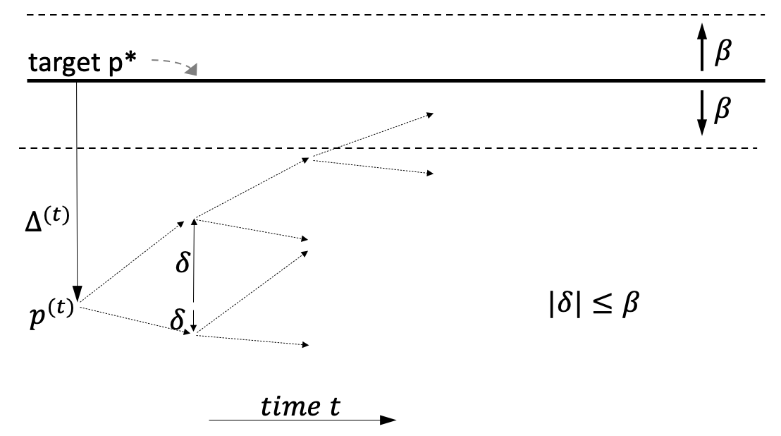
(a) Convergence to within the band (from below in this picture).

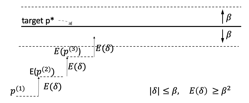
(b) Expected steps and expected positions

Figure 21: A picture of the properties in Lemma 3, upper bounding the expected number of time steps to enter the band ${p^{*}}\pm\beta$ by $\beta^{-2}$, whether from below or above the band (Theorem 1), where $\Delta^{(t)}:={p^{*}}-\hat{p}^{(t)}$ and $\delta^{(t)}:=|\Delta^{(t)}|-|\Delta^{(t+1)}|$. (a) At any point, there are two outcomes after an update (weaken or boost), and the movement, $\delta$, could be toward or away from ${p^{*}}$ (e.g. $\delta<0$), but always $|\delta|\leq\beta$. (b) As long as $\hat{p}$ is not in the band, there is an expected movement, $\mathbb{E}(\delta)$, of at least $\beta^{2}$, toward ${p^{*}}$. $\mathbb{E}(\delta)$ is smallest when $\hat{p}$ is near ${p^{*}}$ and largest, up to $\beta$, when $\hat{p}$ is farthest ($\hat{p}=0$ or $\hat{p}=1$).

Note that from property 2 above, there is always progress towards ${p^{*}}$ in expectation, meaning that if $\hat{p}^{(t)}<{p^{*}}$, then $E(\hat{p}^{(t+1)})>\hat{p}^{(t)}$, and if $\hat{p}^{(t)}>{p^{*}}$, then $E(\hat{p}^{(t+1)})<\hat{p}^{(t)}$. This is the case even if the probability of moving away is higher than $0.5$ ($\hat{p}\leq{p^{*}}<0.5$). We note however, that the result being in expectation, both the actual outcomes for $\hat{p}^{(t+1)}$ can be father from ${p^{*}}$ than $\hat{p}^{(t)}$ (consider when $\hat{p}^{(t)}={p^{*}}$). Property 3 puts a floor (a minimum) on amount of the progress towards ${p^{*}}$ in expectation, when $\hat{p}\not\in[{p^{*}}-\beta,{p^{*}}+\beta]$, For instance, when $\hat{p}^{(t)}\leq{p^{*}}-\beta$ , it puts a minimum on the expected positions $\mathbb{E}(\hat{p}^{(t+1)}),\mathbb{E}(\hat{p}^{(t+2)}),\mathbb{E}(\hat{p}^{(t+3)}),\cdots$, until one such point crosses the band, Fig. 21(b), and Theorem 1 follows.

Theorem.

EMA, with a fixed rate of $\beta\in(0,1]$, has an expected first-visit time bounded by $O(\beta^{-2})$ to within the band ${p^{*}}\pm\beta$. The required number of updates, for first-visit time, is lower bounded below by $\Omega(\beta^{-1})$.

Proof.

We are interested in maximum of first-time $k$ when the expected $\mathbb{E}(\hat{p}^{(k)})\in[{p^{*}}-\beta,{p^{*}}+\beta]$. Using the maximum movement constraint, as long as $|{p^{*}}-\hat{p}^{(t)}|>\beta$, an EMA update does not change the sign of ${p^{*}}-\hat{p}^{(t)}$ ($\hat{p}$ does not switch sides wrt ${p^{*}}$, e.g. if greater than ${p^{*}}$, it remains greater after the update). Thus, before an estimate $\hat{p}^{(t)}<{p^{*}}$ changes sides, and exceed ${p^{*}}$, it has to be within or come within the band ${p^{*}}\pm\beta$. Therefore, start with an arbitrary location $\hat{p}^{(1)}$ outside the band, say $\hat{p}^{(1)}<{p^{*}}-\beta$ (similar arguments apply when $\hat{p}^{(1)}>{p^{*}}+\beta$), and consider the sequence, $\hat{p}^{(1)},\hat{p}^{(2)},\hat{p}^{(3)},\cdots,\hat{p}^{(k)}$, where $\forall t,1\leq t\leq k,\hat{p}^{(t)}<{p^{*}}-\beta$. We can now lower bound the expected position of $\hat{p}^{(k)},k\geq 2$ wrt $\hat{p}^{(1)}$, to be at least $(k-1)\beta^{2}$ above $\hat{p}^{(1)}$:

$$\mathbb{E}(\hat{p}^{(k)}-\hat{p}^{(1)}|\hat{p}^{(1)}=p) =\mathbb{E}(\hat{p}^{(k)}-\hat{p}^{(k-1)}+\hat{p}^{(k-1)}-\hat{p}^{(1)}|\hat{p}^{(1)}=p)$$

$$=\mathbb{E}(\sum_{2\leq t\leq k}\hat{p}^{(t)}-\hat{p}^{(t-1)}|\hat{p}^{(1)}=p)\mbox{\ \ (insert all intermediate sequence members)}$$

$$=\sum_{2\leq t\leq k}\mathbb{E}(\hat{p}^{(t)}-\hat{p}^{(t-1)}|\hat{p}^{(1)}=p)\geq(k-1)\beta^{2},$$

where we used the linearity of expectation, and the $\beta^{2}$ lower bound for the last line. With ${p^{*}}\leq 1$, an upper bound of $\frac{1}{\beta^{2}}$ on maximum first-visit time follows: $k$ cannot be larger than $\frac{1}{\beta^{2}}$ if we want to satisfy $\forall 1\leq t\leq k,\mathbb{E}(\hat{p}^{(t)})<{p^{*}}-\beta$, or one of $t\in\{1,\cdots,\frac{1}{\beta^{2}}+1\}$ has to be within the band ${p^{*}}\pm\beta$.

The lower bound $\Omega(\beta^{-1})$ on $k$ follows from the upperbound of $\beta$ on any advancement towards ${p^{*}}$. ∎

The movement of the estimates $\hat{p}^{(t)}$ can be likened to the motion of a vertically hung spring in some respects: the expected movement is 0 at target ${p^{*}}$, corresponding to the resting length of the spring, or its equilibrium length, where spring acceleration is 0, and the expected movement is highest at the extremes (farthest from ${p^{*}}$), akin to the acceleration (vector) of the spring being highest when its stretched or compressed.

Appendix C Further Material on the Qs (Queues) Method

We begin by reviewing a few properties of a single completed cell of a queue in the Qs method, which is equivalent to the experiment of tossing a biased two-sided coin, with unknown heads PR ${p^{*}}>0$ (the target of estimation), counting the tosses until and including the first heads outcome. We can repeat this experiment until we get $k\geq 1$ heads outcomes. The count in each completed cell follows the geometric distribution, and the total number of trials, or the total count over all completed cells, minus the number of heads, has the more general negative binomial distribution (with parameters $k$ and ${p^{*}}$). In the next section we look at estimators for ${p^{*}}$ using counts from several completed cells, and describe how the general method of Rao-Blackwellization can be applied there to get a superior estimate, in a sense described next.

Ideally, we desire estimates that have no or little bias, that is, if we took the average over many repetitions of the same experiment (e.g. by different people using the same data collection technique, and assuming ${p^{*}}$ is not changing), the average over all the estimates would converge to ${p^{*}}$. We also prefer low variance, implying that any particular estimate in time has low chance of being far from target. The two estimation goals are often distinct, for instance an estimator can have zero variance (fully stable) but nonzero bias, and different ways of collecting data and estimation techniques can exhibit these tradeoffs. We observe, for instance, that the bias of a (MLE) technique below gets worse, in the ratio sense, as the target ${p^{*}}\rightarrow 0$.

C.1 A Single Completed Queue Cell

With $C$ denoting random variable (r.v.) for the count in a completed cell of a queue, in the binary iid setting (Sect. 2.1.3 and 5.3), the expectation of the estimate $X=\frac{1}{C}$ for ${p^{*}}\in(0,1]$, which is known to be the maximum likelihood estimate (MLE) for the geometric and the more general negative binomial distributions [19, 11, 7], can be expressed as the infinite series below: ${p^{*}}$ of the time, we get a heads outcome on the first toss, and the estimate $\frac{1}{C}$ for ${p^{*}}$ is 1, and $(1-{p^{*}}){p^{*}}$ of the time, we get a single tails and then a heads, and the estimate is $1/2$, and so on. The series is called a geometric-harmonic series, and has a closed form in terms of the natural logarithm:

$$\mathbb{E}(X)=\mathbb{E}(\frac{1}{C})={p^{*}}\frac{1}{1}+(1-{p^{*}}){p^{*}}\frac{1}{2}+(1-{p^{*}})^{2}{p^{*}}\frac{1}{3}+\cdots={p^{*}}\sum_{i\geq 1}(1-{p^{*}})^{i-1}\frac{1}{i}=\frac{-{p^{*}}\ln({p^{*}})}{1-{p^{*}}}$$

From the series, ${p^{*}}+(1-{p^{*}}){p^{*}}\frac{1}{2}+\cdots$, it is seen for ${p^{*}}\in(0,1)$, as all series elements are positive, that $\mathbb{E}(\frac{1}{C})>{p^{*}}$, or the MLE $X=\frac{1}{C}$ is a biased, upper bound, estimate of ${p^{*}}$ in expectation. The ratio $\frac{\mathbb{E}(\frac{1}{C})}{{p^{*}}}=\frac{-\ln({p^{*}})}{1-{p^{*}}}$, and we can verify that this ratio grows unbounded as ${p^{*}}\rightarrow 0$ ( $\lim_{{p^{*}}\rightarrow 0}\frac{-\ln({p^{*}})}{1-{p^{*}}}=+\infty$). At ${p^{*}}=1$, $\mathbb{E}(\frac{1}{C})=1$ and there is no bias, thus the bias, in a relative or ratio to ${p^{*}}$ sense, gets worse as ${p^{*}}$ gets smaller.

We now look at the variance, $\mathbb{V}(X)$ of r.v. $X=\frac{1}{C}$, and how its ratio to ${p^{*}}$ changes as ${p^{*}}$ is reduced. For any r.v. $X$, $\mathbb{V}(X):=\mathbb{E}((X-\mathbb{E}(X))^{2})$, or $\mathbb{V}(X)=\mathbb{E}(X^{2})-(\mathbb{E}(X))^{2}$ (linearity of expectation).

$$\frac{\mathbb{V}(X)}{{p^{*}}}=\frac{\mathbb{E}(X^{2})}{{p^{*}}}-\frac{(-{p^{*}}\ln({p^{*}})/(1-{p^{*}})))^{2}}{{p^{*}}}$$

The limit of the 2nd term, $\frac{{p^{*}}(\ln({p^{*}}))^{2}}{(1-{p^{*}})^{2}}$, as ${p^{*}}\rightarrow 0$, is 0, and for the first term:

$$\mathbb{E}(X^{2})={p^{*}}\frac{1}{1^{2}}+(1-{p^{*}}){p^{*}}\frac{1}{2^{2}}+(1-{p^{*}})^{2}{p^{*}}\frac{1}{3^{2}}+\cdots={p^{*}}\sum_{i\geq 1}(1-{p^{*}})^{i-1}\frac{1}{i^{2}}$$

$$\Rightarrow\lim_{{p^{*}}\rightarrow 0}\frac{\mathbb{E}(X^{2})}{{p^{*}}}=\lim_{{p^{*}}\rightarrow 0}\sum_{i\geq 1}(1-{p^{*}})^{i-1}\frac{1}{i^{2}}=\sum_{i\geq 1}\frac{1}{i^{2}}=\frac{\pi^{2}}{6}$$

The last step is from the solution to the Basel problem. Therefore, $\lim_{p\rightarrow 0}\frac{\mathbb{V}(X)}{{p^{*}}}=\frac{\pi^{2}}{6}.$ We note that at ${p^{*}}=1$, the variance is 0 (as $\mathbb{E}(X)=1$, and also $\mathbb{E}(X^{2})=1$ from the series above). So the ratio of variance to ${p^{*}}$, the relative variance, grows but is bounded as ${p^{*}}\rightarrow 0$. That the variance goes up is consistent with the observation that rates of violation also go up, as ${p^{*}}$ is reduced, in Table 3 (using a similar estimator), and Table 4 on performance of Qs (using 5 and 10 queue cells).

C.2 Multiple Completed Cells: Rao-Blackwellization

We have $k\geq 2$ completed queue cells, with $C_{i}$ denoting the count of cell $i,1\leq i\leq k$, or repeating the experiment toss-until-heads $k$ times. We first sketch the Rao-Blackwellization (RB) derivation for an unbiased minimum variance estimate, then briefly look at a few related properties and special cases.

Let the (good) estimate $G_{k}=\frac{k-1}{(\sum_{1\leq i\leq k}C_{i})-1}$. The RB technique establishes that this is an unbiased estimate, i.e. $\mathbb{E}(G_{k})={p^{*}}$, and moreover it is the minimum variance unbiased estimate (MVUE) [32]. We begin with the simple and unbiased but crude estimate $\Theta_{1}=[[C_{1}=1]]$, where we are using the Iverson bracket: ${p^{*}}$ of the time $\Theta_{1}$ is $1$ (the first toss is heads), and otherwise $\Theta_{1}=0$, thus indeed $\mathbb{E}(\Theta_{1})={p^{*}}$. This estimate is crude (highly variant) as it ignores much information such as the other counts $C_{i},i\geq 2$, and we can use RB to derive an improved estimate from $\Theta_{1}$. Let $Y=\sum_{i=1}^{k}C_{i}$ ($Y$ is the total number of tosses), $Y\sim$ NB($k,{p^{*}}$), i.e. $Y$ has the negative binomial distributions with parameters $k$ and ${p^{*}}$. $Y$ is a sufficient statistic for $\Theta_{1}$ [32, 7]. Then the RB estimator is the conditional expectation $\mathbb{E}(\Theta_{1}|Y)$, and because $\Theta_{1}$ is unbiased, this estimator is also unbiased as conditioning does not change bias status and can only improve the variance, and as $Y$ is a sufficient statistic, this estimate is in fact the MVUE [38, 5, 22], and can be simplified to:

$$\mathbb{E}(\Theta_{1}|Y=y)=P(C_{1}=1|Y=y)=\frac{k-1}{y-1}\hskip 28.45274pt\mbox{(Rao-Blackwellization of the crude $\Theta_{1}:=[[C_{1}=1]]$)}$$

where we know that the last coin toss is always a heads (from our data collection set up) and this leaves $k-1$ heads and $y-1$ unaccounted-for tosses. Take the case of $k=2$ cells or heads. The last heads is fixed, and the first one has $y-1$ positions to pick from, all equally likely, thus $P(C_{1}=1|Y=y)=\frac{1}{y-1}$ when $k=2$. More generally for $k\geq 2$, as the tosses are exchangeable with this conditioning, i.e. throwing $k-1$ balls into $y-1$ bins (each bin can contain 1 ball only), the probability that one falls in bin 1 is $\frac{k-1}{y-1}$.

With $k=2$ completed cells (thus $Y\geq 2$), one can show that the estimate $\frac{1}{Y-1}$ is unbiased more directly (but the property of minimum variance is stronger in above):

$$\mathbb{E}(\frac{1}{Y-1})=\sum_{i\geq 2}\frac{P(Y=i)}{i-1}=\sum_{i\geq 2}\frac{(i-1){p^{*}}^{2}(1-{p^{*}})^{i-2}}{i-1}={p^{*}}^{2}\sum_{i\geq 2}(1-{p^{*}})^{i-2}={p^{*}}$$

where, $P(Y=i)=(i-1){p^{*}}^{2}(1-{p^{*}})^{i-2}$, as there are $i-1$ possibilities for the first heads outcome, each having equal probability ${p^{*}}^{2}(1-{p^{*}})^{i-2}$, and the last equality follows from simplifying the sum of the geometric series ($\sum_{i\geq 0}r^{i}=\frac{1}{1-r}$, for $r\in(0,1)$).

From the RB estimator, it follows that $\mathcal{U}_{k}=\frac{k}{Y}$ and $\mathcal{L}_{k}=\frac{k-1}{Y}$ (where $Y:=\sum_{i=1}^{k}C_{i}$ as in above) with increasing $k$ form a sequence respectively of upper bounds and lower bounds, in expectation, for ${p^{*}}$: $\mathbb{E}(\mathcal{L}_{k})<{p^{*}}<\mathbb{E}(\mathcal{U}_{k})$. That the estimate $\mathcal{U}_{k}$ is biased positive can also be seen from an application of Jensen’s inequality [8], using linearity of expectation on the sum of r.v.’s, and the fact that $\mathbb{E}(C_{i})=\frac{1}{{p^{*}}}$ (the mean of the geometric distribution, which can be verified by writing the expectation expression), as follows: Jensen’s inequality for expectation is $f(\mathbb{E}(X))<\mathbb{E}(f(X))$, where the strict inequality holds when these two conditions are met, 1) r.v. $X$ has finite expectation and positive variance (true, in our case, when ${p^{*}}<1$), and 2) $f(x)$ is strictly convex. In our case, $f(x)=\frac{1}{x}$ (a strictly convex function). For one completed cell, we have $f(\mathbb{E}(X))=f(\mathbb{E}(C_{1}))=f(\frac{1}{{p^{*}}})={p^{*}}$, therefore, using Jensen’s inequality, ${p^{*}}<\mathbb{E}(f(X))=\mathbb{E}(\frac{1}{C_{1}})$. Similarly, for $k\geq 2$, $f(\mathbb{E}(Y))=f(\mathbb{E}(\sum C_{i}))=f(\frac{k}{{p^{*}}})=\frac{{p^{*}}}{k}$. And $\mathbb{E}(f(Y))=\mathbb{E}(\frac{1}{Y})$, therefore (via Jensen’s), ${p^{*}}<k\mathbb{E}(\frac{1}{Y})=\mathbb{E}(\mathcal{U}_{k})$.

C.3 Multiple Queues: PR Sums and the Spread of PRs

Unlike EMA, with its particular weakening step, even though the Qs method also has in effect a weakening step (a negative update), the PR estimates from all the queues of a Qs predictor do not form a DI or even an SD, as the sum can exceed 1.0. Sect. 5.5 gave an example, and here we delve deeper. Let $Q$ denote the item to (raw) PR from the Qs method, i.e. before any normalizing (and at any time point). When we feed $Q$ to FC(), scaling is performed to ensure a SD is extracted. In effect, FC() normalizes by the sum. How large does $\mbox{sum}(Q)$ get, violating the SD property, in the worst case? Assume each queue had one cell only, and we used the MLE, $\frac{1}{C_{0}}$, and the stream is composed of $n$ unique items (and with no pruning): then the PR estimates are 1 (for the latest observed item), 1/2 (next to latest), 1/3, and so on, and $\mbox{sum}(Q)$ has the growth rate of a harmonic series, which for $n$ (unique) items, is approximately $\ln(n)+0.577$ (0.577 is called the Euler-Mascheroni constant).

While $\mbox{sum}(Q)$ can be above 1.0, a related question is about the form and spread of the PRs in $Q$. For instance, can $Q$ contain 3 or more PRs equal to $\frac{1}{2}$, or 4 or more $\frac{1}{3}$ PRs , violating the SD property by having too many PRs? Given a threshold $p$, e.g. $p=P_{min}$, let

$$N(Q,p):=|\{i|Q(i)\geq p\}|.\mbox{}$$ (16)

$N(Q,p)$ appears substantially more constrained than $\mbox{sum}(Q)$, as we will see below. $N(Q,p)$ is of interest when we want to use the raw PR values in $Q$ from a Qs technique, and do not want to necessarily normalize $Q$ at every time $t$, for instance for the efficient sparse-update time-stamp Qs method when keeping many PRs for millions of items (Sect. 5.8). If the PRs formed a SD , then $\frac{1}{p}$ would be the bound. In the simpler case of Qs with qcap $=1$ and using the MLE $\frac{1}{C_{0}}$, we can show the same constraint $\frac{1}{p}$ holds, the next lemma below. Note that when pruning the $qMap$ we are in effect using the MLE with qcap $=1$, thus understanding its properties is motivated from the pruning consideration as well.

Let the denominator of PR $Q(i)$ be denoted by $Y_{i}$. In the case of MLE with qcap $=1$, $Y_{i}$ is $C_{0}$, and more generally it is the sum of cell counts. $Y_{i}^{(t)}$ denotes the value at time $t$.

Lemma 7.

For the Qs technique with qcap $=1$, using the MLE $\frac{1}{C_{0}}$, we have the following properties at any time point $t\geq 2$ (on any input sequence):

1. $Y_{i}^{(t)}=1$ if $i$ was observed at time $t-1$, and otherwise $Y_{i}^{(t)}=Y_{i}^{(t-1)}+1$.

2. There is exactly one item $i$ with $Y_{i}^{(t)}=1$ and thus PR $Q^{(t)}(i)=1$, the item observed at $t-1$. For any integer $k\geq 2$, there is at most one item with $Y_{i}^{(t)}=k$ or PR $Q^{(t)}(i)=\frac{1}{k}$.

3. For any threshold $p>0$, $N(Q,p)\leq\frac{1}{p}$.

Proof.

Property 1 follows from how the Qs technique allocates new queue cells and increments counts: at each time $t$ exactly one item is observed, its $C_{0}$ initialized to one upon update, it thus gets a PR of $1$ at $t+1$. Any other item $i$ in the map $Q$ gets its $C_{0}$ incremented, to 2 or higher, or $Y_{i}^{(t)}=Y_{i}^{(t-1)}+1$. Thus exactly one item, the observed item at $t-1$, has $Y_{i}^{(t)}=1$. Property 2 completes using induction on $k\geq 1$, the base case is 1st half of property 2, and for the induction step, we use part 1: Assuming it holds for all integer up to $k\geq 1$, the property for $k+1$ can be established by contradiction: if there are two or more items with $Y^{(t)}=k+1$, these items must have had $Y^{(t-1)}=k$ (neither could have been observed at $t-1$) contradicting the at-most-one property for $k$.

From part 2, it follows that the maximum number of PRs $N(Q,p)$ is $k$ for probability threshold $p=\frac{1}{k}>0$, where $k$ is an integer, $k\geq 1$ (with at most one PR $\frac{1}{j}$, for each $j\in\{1,2,\cdots,k\}$). As all PRs in $Q$ are limited to integer $\frac{1}{k}$ fractions (the harmonic numbers), the constraint remains $\frac{1}{p}$ for any threshold $p>0$ (not just integer fractions). ∎

We next explore similar properties when using more cells, and where we use the GetPR() function in the Qs technique (Fig. 8). Let $q(i)$ be short for $qMap(i)$, i.e. the queue for $i$ (when the queue exists). Thus for item $i$, the PR $Q(i)$ is GetPR($q(i)$). Here, with several cells, we need to use the count for cell0, $C_{0}$, e.g. we use the estimate $Q(i)=\frac{1}{C_{0}+C_{1}-1}$ for two cells. Otherwise, if counts from only completed cells, say $C_{1}$ and $C_{2}$ are used (skipping cell0), we can have a worst-case sequence (with non-stationarity) such as $AAABBBCCC\cdots$ (an item never occurs after appearing a few times) where the PR estimates (using only completed cells) for many items are all $1$. Using the partial cell0 breaks this possibility, and we can establish properties similar to above. Let $|q(i)|$ denote the number of cells in the queue, and define $Y_{i}$ to be the denominator used in GetPR(), $Y_{i}:=\sum_{0\leq j<|q(i)|}C_{j}-1$, thus $Q(i)$ is either 0, when there is no queue for $i$, or otherwise $Q^{(t)}(i)=\frac{|q^{(t)}(i)|-1}{Y_{i}^{(t)}}$ ($Q(i)$ can still be 0 when $|q(i)|=1$), where $Y_{i}^{(t)}$ is the denominator and $q^{(t)}(i)$ is the queue of $i$ at $t$.

Lemma 8.

For the Qs technique with qcap $\geq 2$, for any item $i$ with a queue $q(i)$, $|q(i)|\leq$ qcap, using the PR estimate $Q(i)=\frac{|q(i)|-1}{Y_{i}}$, where $Y_{i}:=\sum_{0\leq j<|q(i)|}C_{j}-1$, for any time point $t\geq 1$:

1. $Q^{(t)}(i)$, when nonzero, has the form $\frac{a}{b}$, where $a$ and $b$ are integers, with $b\geq a\geq 1$.

2. If $i$ is not observed at $t$, then $Y_{i}^{(t+1)}=Y_{i}^{(t)}+1$ or $i$ is removed from the map $qMap$. When $i$ is observed at $t$ (exactly one such), then $Y_{i}^{(t+1)}\leq Y_{i}^{(t)}$ when $|q^{(t)}(i)|=$ qcap, and $Y_{i}^{(t+1)}=Y_{i}^{(t)}+1$ when $|q^{(t)}(i)|<$ qcap.

3. If $i$ is observed at $t$, then $Q^{(t+1)}(i)\geq Q^{(t)}(i)$. If $i$ is not observed at $t$, then $Q^{(t+1)}(i)<Q^{(t)}(i)$.

Proof.

Part 1 follows from $Y_{i}$ being an integer, and the Qs technique outputs a non-zero PR only when $|q(i)|>1$, in which case $Y_{i}>0$ (with two or more queue cells), and we also have $|q(i)|-1\leq Y_{i}$ (each queue cell has count of at least 1, therefore, $Y_{i}+1=\sum_{0\leq j<|q(i)|}C_{j}\geq|q(i)|$ ).

Proof of part 2: if an item $i$ in $qMap$ is not observed at $t$ and removed from $qMap$, its count in cell0 is always incremented for $t+1$, i.e. $Y_{i}^{(t+1)}=Y_{i}^{(t)}+1$. Upon observing item $i$ at $t$, when $|q^{(t)}(i)|=$ qcap , one cell is dropped with count $\geq 1$, and one cell is added, thus $Y_{i}^{(t+1)}\leq Y_{i}^{(t)}$, and when $|q^{(t)}(i)|<$ qcap , one cell with count 1 is added, thus $Y_{i}^{(t+1)}=Y_{i}^{(t)}+1$.

Proof of part 3: On a negative update, the denominator of $Q(i)$, $Y_{i}$, always goes up from part 2, while the numerator (or number of queue cells) doesn’t change. On a positive update, when the queue is at capacity, the numerator does not change, while denominator may go down (part 2). When the queue hasn’t reached capacity ($q^{(t)}(i)<$ qcap), both the numerator and denominator go up by 1 each, but as the denominator is never smaller than numerator (part 1), the result is $Q^{(t+1)}(i)\geq Q^{(t)}(i)$. ∎

As property 3 above states, an item’s PR may not change after a positive update: This happens when the item’s queue is at capacity and the last cell of the queue, to be discarded, has a 1 (one count-one cell is dropped, but another such is added at the back, and $Y_{i}$ is not changed). The other case for no change is when $Q(i)=1$ already (which can occur after several consecutive observations of the item).

With qcap $>2$, there can be $N(Q,p)>\frac{1}{p}$. For instance, with qcap of 4, on the sequence of $AAAABB$, item $A$ reaches $Q(A)=1$ at $t=3$ (after the update at $t=2$) through $5$, and goes down to $3/5$ at $t=7$, while $B$ reaches 1 at the $t=7$, thus with threshold $p=3/5$, $N(Q^{(7)},p)=2>\frac{1}{p}=5/3$.

Let us call the variant of Qs as the uniform Qs technique where $Q(i)=0$ item $i$ while $|q(i)|<$ qcap, i.e. wait until queue of $i$ has reached its capacity. Note that plain Qs with qcap of 2 is already uniform.

Lemma 9.

For the uniform Qs technique with qcap $=a$, integer $a\geq 2$, consider items $i$ with $Q(i)>0$ (i.e. queue $q(i)$ exists and $|q(i)|=a$), where the PR estimate $Q(i)=\frac{a-1}{Y_{i}}$ is used. At any time point $t\geq 1$:

1. For any integer $k\geq a-1$, there are at most $k$ items with $Y_{i}^{(t)}\leq k$ among items $i$ such that $Q^{(t)}(i)>0$.

2. For any threshold $p>0$, $N(Q,p)\leq\lceil\frac{a-1}{p}\rceil$.

Proof.

(part 1) Proof by induction on $k$, the base case being $k=a-1$. let $S_{k}$ denote the set of items with $Y_{i}\leq k$. For the base case, we must have $t\geq a$, as before $t=a$ no item has $Q(i)>0$. We can verify that an item that gets $a$ consecutive positive updates satisfies this constraint, and no other item, and there can be at most one such item at any time $t$ (any other item has at least one negative update, so $Y_{i}\geq a$ for such). Thus $|S_{a-1}|\leq 1$. For the induction step, assuming the constraint holds for up to $k\geq a-1$, i.e. $S_{k}\leq k$, we need to show it holds for $k+1$. We do this by induction on $t\geq a$, where the base case is that it holds for all $k$ at $t=a$. To show this holds for $t+1$, if there are no items at $t$ with $Y_{i}=k+1$, then we must have $k$ or fewer with $Y_{i}\leq k$, i.e. $|S^{(t)}_{k+1}|\leq k$, and at $t+1$, the items in $S^{(t)}_{k+1}$ will all be in $S^{(t+1)}_{k+1}$, and possibly one additional item, the one with a positive update, is added to $S^{(t)}_{k+1}$, thus $|S^{(t+1)}_{k+1}|\leq|S^{(t)}_{k+1}|+1\leq k+1$ (at $t+1$). If we have one or more at $t$ with $Y_{i}=k+1$, all except one have a negative update at $t$, leaving the ones $S^{(t)}_{k}$, $|S^{(t)}_{k}|\leq k$ for $S^{(t)}_{k+1}$, thus $|S^{(t+1)}_{k+1}|\leq k+1$ (at most one other item is added, either one with $Y_{i}=k+1$, or another item $i\not\in S^{(t)}_{k+1}$).

(part 2) Given threshold $p>0$, let $S^{(t)}_{p}=\{i|Q^{(t)}(i)\geq p\}$, or $S^{(t)}_{p}=\{i|\frac{a-1}{Y_{i}^{(t)}}\geq p\}=\{i|\frac{a-1}{p}\geq Y_{i}^{(t)}\}$. Therefore, from part 1, $|S^{(t)}_{p}|\leq\lceil\frac{a-1}{p}\rceil$. ∎

The bound $\lceil\frac{a-1}{p}\rceil$ may be significantly loose for $a\geq 3$, and a simple $\frac{1}{Y_{i}}$ may hold (i.e. independent of qcap ), or it would be good to find examples violating the bound $\frac{1}{Y_{i}}$. Studying how the negative updates affect the sums $Y_{i}$ should be fruitful. For the plain (non-uniform) Qs technique, we also conjecture that $N(Q,p)<\frac{a}{p}+$ qcap , i.e. the constraint on $N(Q,p)$ can be violated by no more than an extra (additive) $qcap$. In the case of qcap of 2, like the case of Lemma 7 (using one cell and the MLE), the (positive) PRs in $Q(i)$ are harmonic fractions, but there is more variation here compared to MLE with qcap of 1 case. For instance, it is possible that no item gets PR of 1 at certain time points $t\geq 2$, while we can have two items with PR $\frac{1}{2}$, and in general, up to $k$ items with PR $\frac{1}{k}$, at which case we get a perfect DI (the sum adds to 1). In other cases, such as the sequence $AABBCCDD\cdots$, the sum can exceed 1 substantially. The underlying cause for violating the DI property is that different items have different starting time points (to keep a bounded memory while reacting to new items, and non-stationarities), thus one recent item from its frame of reference can have PR of 1 (item $D$ in the example $[AABBCCDD]$), while simultaneously, another item, seen earlier in time, has a positive PR such as $\frac{1}{2}$ for $C$.

Appendix D Additional Synthetic Experiments

D.1 Tracking One Item

Table 14 reports under the same synthetic setting of Table 5, i.e. tracking the single item 1 in binary sequences, with a few different parameter values: deviation-rates with $d=1.1$ (convergence to within 10%), Qs with qcap of 3 (as DYAL uses this as its default), and DYALwith lower rates. As expected, $d=1.1$ yields high deviation rates, and $O_{min}$ of 50 helps lower the rate for any $d$ and method. Low minimum rates for DYAL (0.0001) help it achieve lowest deviation rates for $d=1.1$.

deviation $\rightarrow$	1.1	1.5	2	1.1	1.5	2	1.1	1.5	2
threshold	Qs, 3			DYAL, 0.1			DYAL, 0.0001
[0.025, 0.25], 10	0.906	0.542	0.277	0.904	0.637	0.496	0.864	0.591	0.408
[0.025, 0.25], 50	0.907	0.539	0.265	0.900	0.625	0.476	0.529	0.167	0.088
$\mathcal{U}(0.01,1.0)$, 10	0.877	0.522	0.282	0.894	0.615	0.463	0.890	0.562	0.351
$\mathcal{U}(0.01,1.0)$, 50	0.873	0.507	0.263	0.849	0.563	0.424	0.750	0.303	0.156
	Static EMA, 0.1			Static EMA, 0.01			DYAL, 0.01
[0.025, 0.25], 10	0.898	0.619	0.469	0.827	0.510	0.357	0.813	0.481	0.329
[0.025, 0.25], 50	0.896	0.604	0.451	0.680	0.257	0.128	0.673	0.247	0.126
$\mathcal{U}(0.01,1.0)$, 10	0.892	0.608	0.446	0.926	0.684	0.478	0.896	0.583	0.360
$\mathcal{U}(0.01,1.0)$, 50	0.847	0.543	0.404	0.830	0.400	0.206	0.786	0.315	0.143

Table 14: As in Sect. 7.2, for an additional evaluation setting ($d=1.1$) and algorithm parameters.

Table 15 repeats the uniform-setting experiments of Table 5, but with the extra constraint that each stable period be at least 1000 time points.

deviation $\rightarrow$	1.5	2	1.5	2
threshold	Qs, 5		Qs, 10
$\mathcal{U}(0.01,1.0)$, 10	0.226 $\pm$ 0.036	0.064 $\pm$ 0.023	0.103 $\pm$ 0.035	0.021 $\pm$ 0.020
$\mathcal{U}(0.01,1.0)$, 50	0.233 $\pm$ 0.049	0.052 $\pm$ 0.022	0.102 $\pm$ 0.029	0.023 $\pm$ 0.022
	static EMA, 0.01		static EMA, 0.001
$\mathcal{U}(0.01,1.0)$, 10	0.093 $\pm$ 0.045	0.041 $\pm$ 0.023	0.487 $\pm$ 0.114	0.271 $\pm$ 0.117
$\mathcal{U}(0.01,1.0)$, 50	0.099 $\pm$ 0.051	0.043 $\pm$ 0.028	0.462 $\pm$ 0.149	0.311 $\pm$ 0.164
	Harmonic EMA, 0.01		Harmonic EMA, 0.001
$\mathcal{U}(0.01,1.0)$, 10	0.094 $\pm$ 0.052	0.038 $\pm$ 0.018	0.413 $\pm$ 0.125	0.237 $\pm$ 0.105
$\mathcal{U}(0.01,1.0)$, 50	0.125 $\pm$ 0.084	0.050 $\pm$ 0.028	0.364 $\pm$ 0.161	0.241 $\pm$ 0.144
	DYAL, 0.01		DYAL, 0.001
$\mathcal{U}(0.01,1.0)$, 10	0.048 $\pm$ 0.023	0.025 $\pm$ 0.024	0.100 $\pm$ 0.039	0.039 $\pm$ 0.034
$\mathcal{U}(0.01,1.0)$, 50	0.074 $\pm$ 0.060	0.022 $\pm$ 0.031	0.084 $\pm$ 0.044	0.036 $\pm$ 0.019

Table 15: Repeating the uniform setting of Table 5 but with the extra constraint that each stable period be at least 1000 time points. The deviation rates are averages over 20 sequences. Deviation rates substantially improve (compared to Table 5), because the stable periods are uniformly longer.

D.2 Multiple Items, $P_{max}=0.1$

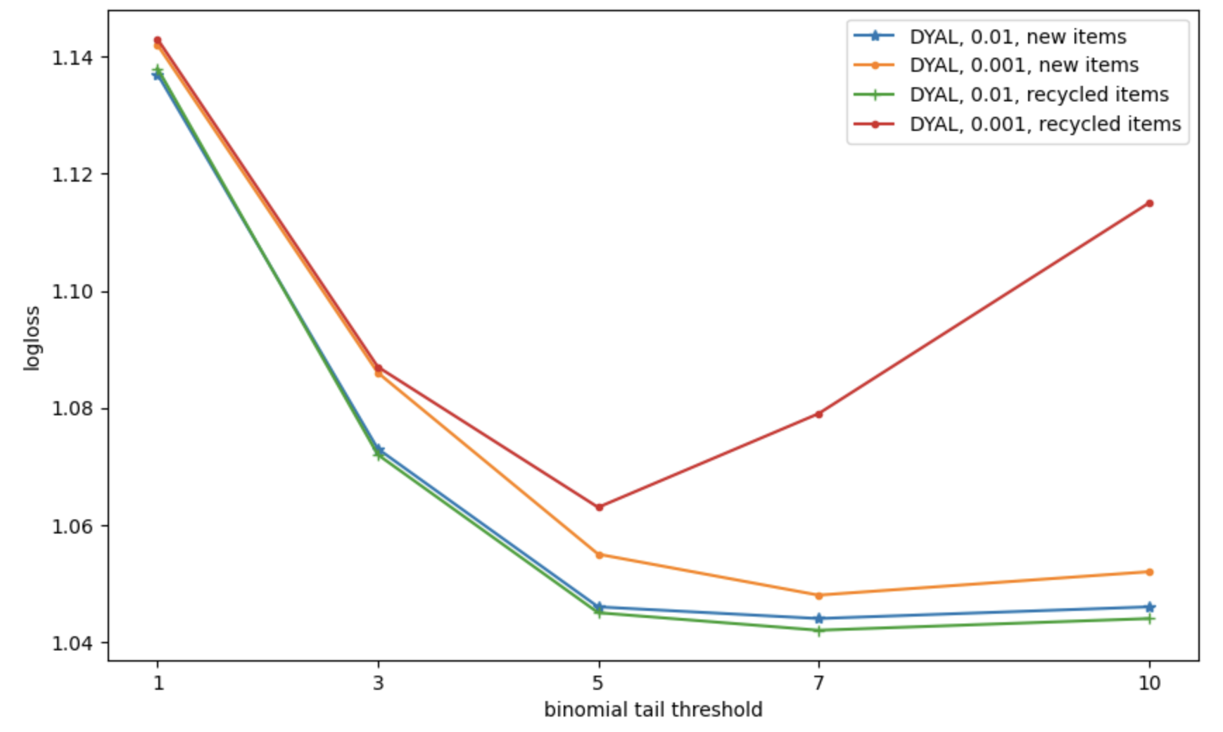
(a) loss vs binomial tail in DYAL

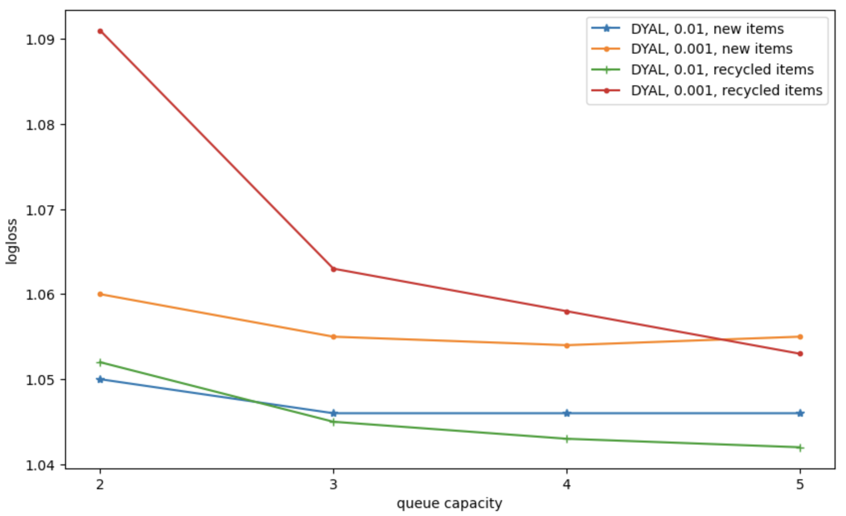
(b) loss vs queue qcap in DYAL

Figure 22: Sensitivity of DYAL to parameters, in synthetic multi-item setting: (a) binomial tail threshold (controlling when to swtich to queues) (b) the queue capacity qcap . These are same 50 sequences as described in Table 6, under both new-item and recycle generation settings, and with $O_{min}=50$).

Table 16 presents multi-item synthetic experiments with $P_{max}=0.1$ when generating the underlying true $\mathcal{P}$ (GenSD()). Average number of different SDs, generating a sequence, in these experiments is around 3 with $O_{min}=50$, and around 13 with $O_{min}=10$. We observe similar patterns to Table 6 in that DYAL is less sensitive to the choice of $\beta_{min}$, and is competitive with the best of other EMA variants. Compared to Table 6, with overall lower PRs for the salient items and in a narrower range (0.01 to 0.1), the log-loss perfromances are worse, and static EMA with $\beta=0.01$ is more competitive with DYAL. Paired experiments and counting the number of wins show that DYAL with $\beta_{min}=0.01$ beats the best of others convincingly, in Table 17, while DYAL with $\beta_{min}=0.001$ struggles compared to other EMA variants with $\beta=0.01$.

	1.5any	1.5obs	logloss	1.5any	1.5obs	logloss	opt. loss
new items $\downarrow$	Qs, 5			Qs, 10
10, [0.01, 0.1]	1.00	0.46	3.02	1.00	0.40	3.05	2.84 $\pm$0.02
50, [0.01, 0.1]	1.00	0.41	2.94	0.99	0.24	2.91	2.83 $\pm$0.04
	static EMA, 0.01			static EMA, 0.001
10, [0.01, 0.1]	1.00	0.28	3.02	1.00	0.75	3.68	2.84
50, [0.01, 0.1]	0.99	0.19	2.89	0.73	0.22	3.07	2.83
	harmonic EMA, 0.01			harmonic EMA, 0.001
10, [0.01, 0.1]	1.00	0.28	3.02	1.00	0.75	3.70	2.84
50, [0.01, 0.1]	0.99	0.19	2.89	0.71	0.22	3.07	2.83
	DYAL, 0.01			DYAL, 0.001
10, [0.01, 0.1]	1.00	0.28	3.01	0.98	0.27	3.11	2.84
50, [0.01, 0.1]	1.00	0.20	2.88	0.73	0.07	2.88	2.83
recycle items $\downarrow$	Qs, 5			Qs, 10
10, [0.01, 0.1]	1.00	0.41	2.95	0.99	0.26	2.93	2.84 $\pm$0.02
50, [0.01, 0.1]	1.00	0.40	2.94	0.99	0.21	2.89	2.84 $\pm$0.04
	static EMA, 0.01			static EMA, 0.001
10, [0.01, 0.1]	1.00	0.21	2.90	1.00	0.33	2.98	2.84
50, [0.01, 0.1]	1.00	0.18	2.88	0.70	0.11	2.88	2.84
	harmonic EMA, 0.01			harmonic EMA, 0.001
10, [0.01, 0.1]	1.00	0.21	2.90	1.00	0.32	2.98	2.84
50, [0.01, 0.1]	1.00	0.18	2.88	0.67	0.10	2.89	2.84
	DYAL , 0.01			DYAL , 0.001
10, [0.01, 0.1]	1.00	0.22	2.90	1.00	0.30	2.95	2.84
50, [0.01, 0.1]	1.00	0.18	2.88	0.65	0.08	2.87	2.84

Table 16: Here, $P_{max}=0.1$ for GenSD() (instead of 1.0), and otherwise, as in Table 6: averages over 50 sequences, about  10k length each, $O_{min}$ of 10 and 50 (1st column of the table), unifrom sampling of ${p^{*}}$ in [0.01, 0.1], and changing the SD whenever all items are observed $O_{min}$ times.

DYAL vs. $\rightarrow$	Qs, 10	static, 0.01	harmonic, 0.01	Qs, 10	static, 0.01	harmonic, 0.01
vs. DYAL , 0.001	new items			recycle items
10, 0.01, [0.01, 0.10]	50, 0	50, 0	50, 0	50, 0	50, 0	50, 0
50, 0.01, [0.01, 0.10]	0, 50	43, 7	43, 7	0, 50	10, 40	7, 43
vs. DYAL , 0.01	new items			recycle items
10, 0.01, [0.01, 0.10]	0, 50	0, 50	0, 50	0, 50	0, 50	0, 50
50, 0.01, [0.01, 0.10]	0, 50	0, 50	0, 50	0, 50	0, 50	0, 50

Table 17: Number of wins in ’paired’ experiments, in the setting of Table 16): the 2nd number in each pair is the number of wins of DYAL (when log-loss lower), on the same set of 50 sequences (each  10k). For instance, in top left cell, Qs with qcap =10 beats DYAL when $O_{min}=10$, on all 50 sequences, and loses on all 50 sequences when $O_{min}=50$ (cell below). DYAL with $\beta_{min}=0.01$ beats all others.

Appendix E Further Material on Real-World Experiments

Descriptions of the methods used for concept composition and interpretation within the simplified Expedition system.

E.1 Simplified Interpretation

Each interpretation episode begins at the character level. We do a “bottom-up” randomized search, where we repeatedly pick a primitive concept and invoke and match its holonyms to the input line, near where the invoking concept has matched, until there are no holonyms or no holonyms match. We only do exact match here, i.e. no approximate matching ("ab" matches if both "a" and "b" are present, with "b" immediately following "a"). We keep the top two concepts along a bottom-up path, the top-matching concepts. We repeat such bottom to top searched and matches until all characters (positions) in the input line have been covered, i.e. have one or more matching concepts. From the set of matching concepts, the process generates candidate interpretations and selects a final interpretation: a candidate interpretation is a sequence of top-matching concepts (one of the two that are end of each path), covering all the positions (characters) in the input line, and without any overlap, and where two new non-primitive concepts, i.e. below a frequency threshold, cannot be adjacent. When there are several candidate interpretations, we pick one with minimum number of concepts in it, breaking ties randomly.

E.2 Simplified Composition

The simplified concept generation process: in every episode, once the interpretation process is done, one obtains a final interpretation, that is a sequences of concepts (a mix of 1-grams, 2-grams, etc) covering all the characters in the line input to the episode. Note that in the beginning of the entire learning process, when no new concepts are generated, the final interpretation is simply the sequences of primitive concepts corresponding to the characters. Interpretation is easy at the character level (does not involve search).

Adjacent concepts pairs in an interpretation are processed in the following manner to possibly generate new concepts (compositions): Skip the pair with some probability $p_{g}$ (0.9 in our experiments). Otherwise, again skip the pair if either does not meet the minimum observed-count requirement, where we have experimented with 100, 500, and 2000 in our experiments. Otherwise, generate the composition if it does not already exist (a hashmap look up). Therefore, if "a" and "b" are two concepts, with "b" often occurring after "a" in the input (lines or interpretations), with high probability at some point the composition concept "ab" is generated. Note that the generation probability $p_{g}$ as well as the threshold on frequency affect how fast new concepts (items) are generated.

E.3 Discussion: Separation of Prediction from Concept Use

Although we could use the prediction weights to influence the generation and selection of candidate interpretations, we use the above simple interpretation and concept generation methods to completely divorce prediction weight learning from the trajectory of concept generation and use, and to simulate internal non-stationarity. We note that the bigrams and the higher n-grams that are generated and used have good quality. For instance, when we define a split location, the boundary between two adjacent concepts as good (good split) if it coincides with a blank space (or other punctuation), and bad otherwise (splits within a word), we observe that the ratio of bad to good splits substantially improves over time (e.g. from around 75% to below 30%), as larger concepts are generated and used via the above simple processes (indicating that the larger n-grams learned increasingly correspond to words, phrases, etc.).

Learning and using the predictions should improve the interpretation process, for instance approximate matching and use of predictions are important when there is substantial noise, such as typos in the input text, requiring inference based on larger context to fix. However, in the experiments of this paper, we have separated the processes to more easily compare different prediction (weight learning) techniques.

E.4 Further Evidence of Stationarity vs. Non-Stationarity

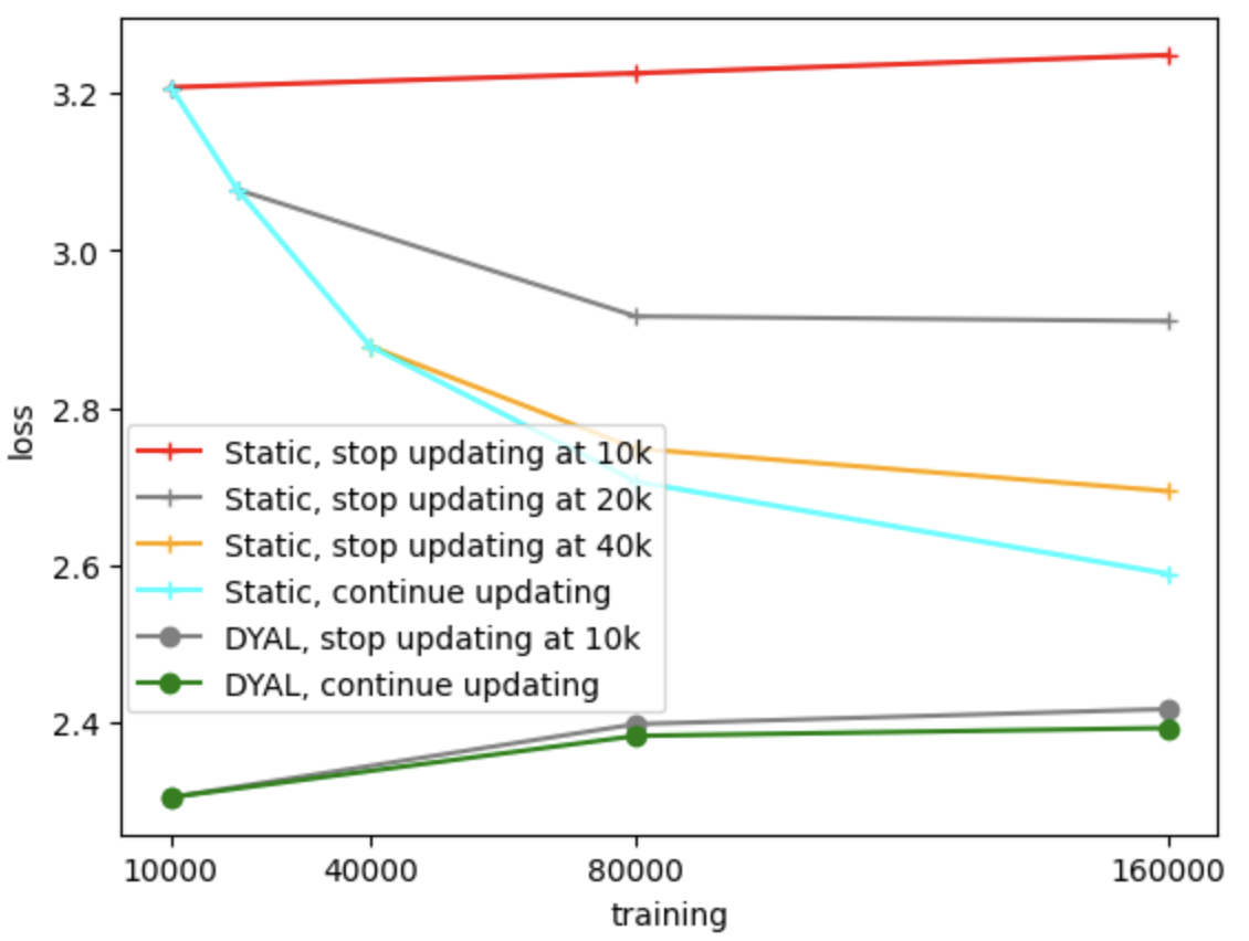
(a) Expedition, remain at character level.

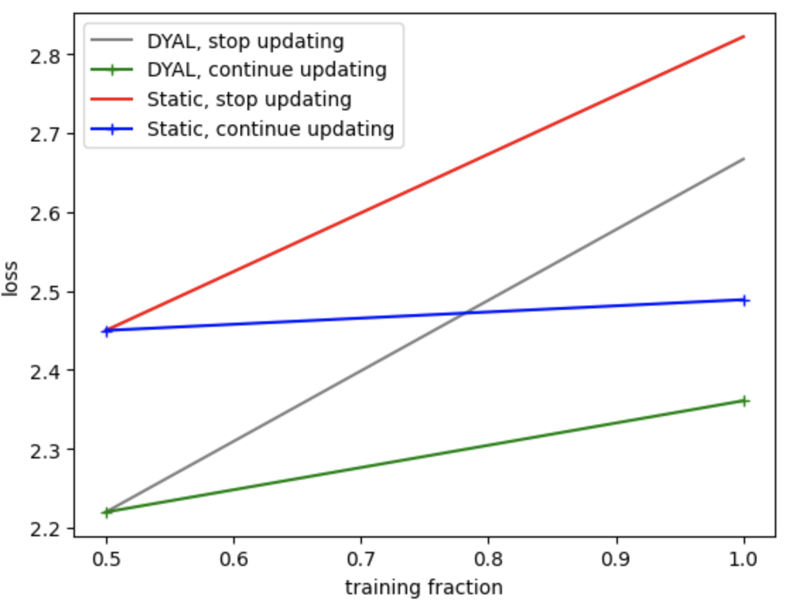
(b) 52-scientists (Unix sequences).

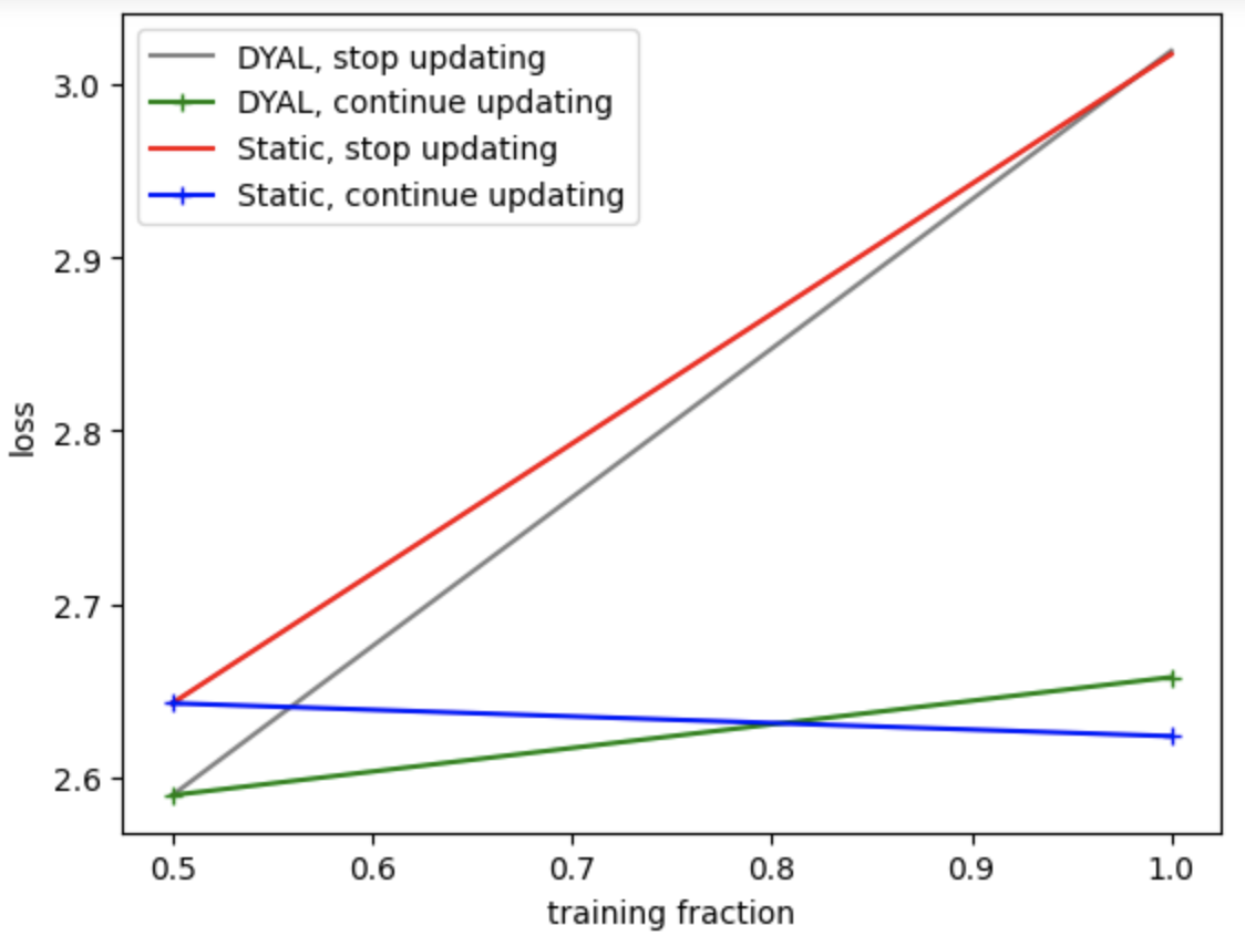
(c) Masqurade (Unix sequences).

Figure 23: Performances (log-loss) when we stop the learning at certain time $t$ vs. continued updating (continuing learning). (a) On the stationary character-level prediction. (b) and (c) on Unix sequences: Continuing the updates vs. stopping the updates at half the sequence length, and measuring performance at that point and once the sequence finishes (averaged log-loss over all the sequences in each data source). When we stop the updates, the performance takes a substantial hit, whether using DYAL or static EMA, on Unix sources, but not on the character-level Expedition.

Fig. 23 shows log-loss performances at two or more time points $t$, comparing performance of continuing to update (continued learning), vs. stopping of the updates (freezing the current weights for prediction on the rest of the sequence).

Fig. 23(a) is on Expedition at character level, the same set up of Sect. 8.2, except that here we may stop the learning at an early point. For static (EMA) and DYAL, using $\beta=0.001$, we stop the updates at time 10k and we compare this to the regime of continuing the updates. We report the loss at 10k and at 80k and 160k. For static, we also included plots when stopping the updates at 20k and 40k. We observe the performance when stopping the updates at say 10k, at 80k or 160k is close (often better) than what it was at 10k, indicating the input distribution has not changed. The plots should be contrasted against Fig. 23(b-c) described next. We suspect the reason the performance of static at times improves, even though we have stopped the updates, is that due to its low fixed learning rate, and that we report the average over all of the times till that point, the effect of latest learning is not fully reflected, and as we allow more time (report log-loss at higher $t$), the result is more reflective of more recent and better performance. For DYAL, its performance converges quickly (by $t$=10k) on this stationary data and the performance only slightly degrades with higher $t$ as some new items are observed (similar to Fig. 19).

For Fig. 23(b) and 23(c), we are comparing continued learning vs. stopping at half the sequence length, on 52-scientists and Masqurade, using static EMA and DYAL with $\beta$ of $0.05$ (similar setting and results to Sect. 8.3.2). For Masqurade, all sequences are 5k long, thus we report (average) performance at $t=$2.5k (the average log-loss performance up to time $t=$2.5k), and then either stop or continue the learning till the end, i.e. $t=$5k, and report performance at 5k as well for both situations. As in previous results, the reported losses (at different time snapshots) are the result of averaging over all the 50 sequences (users) of Masqurade. For 52-scientists, sequences have different lengths, so the times at which we report performances (use for averaging) are sequence dependent. For instance, for a sequence of total length 200, we use the performance at $t=100$, then also use the performances at $t=200$ for the two cases of continued updates and stopping the updates at $t=100$ (and average each over the 52 sequences). We observe that in all cases, whether for DYAL or static EMA, stopping the learning leads to substantial increase in loss compared to continuing the updates (learning), and worse than the average performance at half the length, the latter observation implying presence of (external) non-stationarity. We have tried several learning rates (not just the best performing rate of 0.05), and obtained similar results.

Another way to see evidence of non-stationarity is to look at the max-rate, the maximum of the learning-rate, in the $rateMap$ of DYAL, as a function of time. Whenever the max-rate goes up, it is evidence that an item is changing PR, for instance a new item is being added. Furthermore, here for each sequence, we concatenate it with itself $k$ times, $k=10$ or $k=3$ in Fig. 24. For example, if the original sequence has the three items [A, C] (i.e. $o^{(2)}=$$C$), then the 3x replication (self-concatenation) is [A,C,A,C,A,C]. If the start of a sequence has a distribution substantially different from the ending then, when concatenated, we should repeatedly see max-rate jump up. We looked at 10s of such plots. The max-rate repeatedly go up in plots of all sequences from the 52-scientists (whether with default parameters or with $\beta_{min}$ of 0.05), and all except 1 of the 50 Masqurade sequences, and similar pattern on all except the shortest handful of sequences from 104-Expedition . These short ones are around a 100 time points long, and in the first pass, the predictor learns the distribution and does not need to change it substantially. Fig. 24 shows max-rate on 6 self-concatenated sequences, one example where the max-rate does not change much after the first pass, the other 5 where we see max-rate jumping up repeatedly. These sequences do not necessarily have many (near 100) unique salient items (occurring a few times), implying that in some, there exist salient items with high proportion that are replaced with other such over time. For instance, there are 13 sequences in the 52-scientists with number of items seen 3 or more times below 30. Replicating the longer sequences leads to too many ups in the plots (spikes) to be discernable, such as the right example plot from 52-scientists.

As one concrete example, in one sequence from the 52-scientists, with length 1490, the number of increases in max-rate was 10 on the original sequence, and then 7 increases in all subsequent replications. The times of increase, the command (item) observed, and its rate (changing the maximum rate, and the EMA PR in the first pass were: [(15, ’quit’, ’0.11’, ’0.12’), (28, ’more’, ’0.20’, ’0.25’), (43, ’/bin/pdplk’, ’0.14’, ’0.17’), (59, ’/bin/pdp60’, ’0.07’, ’0.08’), (105, ’pdp60’, ’0.12’, ’0.14’), (170, ’mv’, ’0.20’, ’0.25’), (230, ’rm’, ’0.07’, ’0.07’), (607, ’users’, ’0.33’, ’0.40’), (1408, ’rlogin’, ’0.06’, ’0.12’), (1409, ’quit’, ’0.08’, ’0.17’)], thus at time t=50, the item ’quit’ gets the learning rate of 0.11 (increasing the max-rate) and obtains PR of 0.12. The maximum rate before the increase is often 0.05 (the minimum rate in these experiments). In the 2nd pass, and all subsequent passes, the 7 increase points are: [(1492, ’mail’, ’0.33’, ’0.33’), (1519, ’more’, ’0.17’, ’0.37’), (1601, ’pdp60’, ’0.07’, ’0.15’), (1663, ’mv’, ’0.12’, ’0.29’), (2097, ’users’, ’0.33’, ’0.40’), (2898, ’rlogin’, ’0.06’, ’0.12’), (2899, ’quit’, ’0.08’, ’0.17’)].

(a) Expedition, sequence 5, original length of 127.

(b) Expedition, sequence 36, original length 684.

(c) 52-scientists, shortest sequence.

(d) 52-scientists, sequence 20.

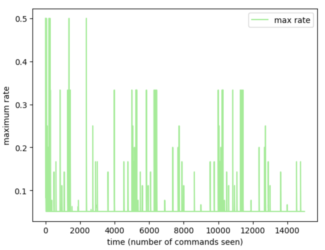
(e) Masqurade, 3x.

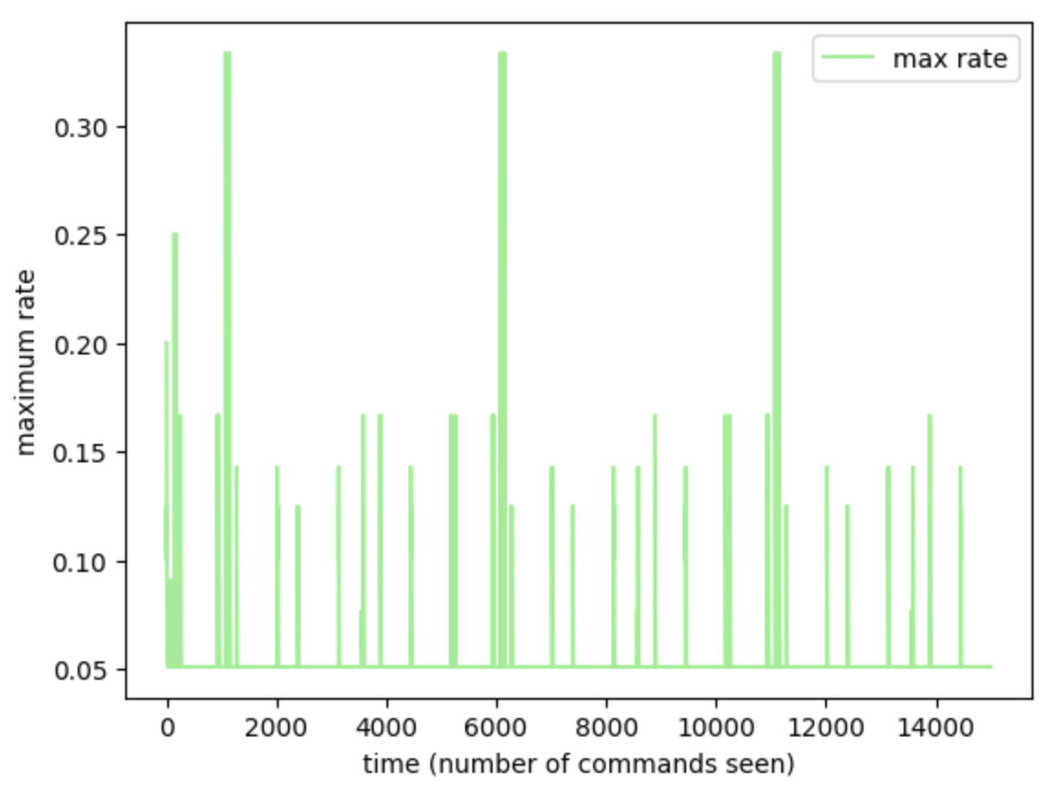
(f) Masqurade, 3x.

Figure 24: The maximum learning rate within DYAL (over the rate map $rateMap$) as a function of time, on two sequences from each of 104-Expedition, 52-scientists, and 50 Masqurade sequences, where each sequence is concatenated with itself 10 times, 3x for Masqurade, thus the length of the original sequence is 127 in top left, but after 10x concatenation, it is 1270 (’sequence 5’ means the 5th shortest sequence). We observe that the max-rate repeatedly jumps up, exhibiting pulsing or spiking patterns, indicating change, except for a handful of very short sequences of the 104-Expedition sequences, and one sequence with only a few unique items from Masqurade.

References

- [1] W. C. Abraham and A. V. Robins. Memory retention – the synaptic stability versus plasticity dilemma. Trends in Neurosciences, 28:73–78, 2005.
- [2] R. Arratia and L. Gordon. Tutorial on large deviations for the binomial distribution. Bulletin of Mathematical Biology, 51:125–131, 1989.
- [3] R. B. Ash. Information Theory. Dover Publications, 1990.
- [4] A. M. Atto, F. Bovolo, and L. Bruzzone. Change Detection and Image Time Series Analysis 1: Unsupervised Methods. Wiley-ISTE, 2021.
- [5] D. Blackwell. Conditional expectation and unbiased sequential estimation. The Annals of Mathematical Statistics, 1947.
- [6] G. W. Brier. Verification of forecasts expressed in terms of probability. Monthly Weather Review, 1950.
- [7] Wikipedia Contributors. The Rao-Blackwell-Kolmogrov Theorem, Jensen’s Inequality, Negative Binomial Distribution, Moving average, Efficiency (statistics), Kalman Filter, and Change Detection. In Wikipedia, The Free Encyclopedia. https://en.wikipedia.org/wiki/.
- [8] T. M. Cover and J. A. Thomas. Elements of Information Theory. John Wiley & Sons, 1991.
- [9] V. Dani, O. Madani, D. Pennock, S. Sanghai, and B. Galebach. An empirical comparison of expert aggregation techniques. In UAI, 2006.
- [10] Thomas L. Dean and Michael P. Wellman. Planning and Control. Morgan Kaufmann, 1991.
- [11] J. L. Devore. Probability and Statistics for Engineering and the Sciences. 9th Edition, Cengage, Boston, 2016.
- [12] H. Du. Beyond strictly proper scoring rules: The importance of being local. Weather and Forecasting, 2020.
- [13] P. Dupont, F. Denis, and Y. Esposito. Links between probabilistic automata and hidden markov models: probability distributions, learning models and induction algorithms. Pattern Recognition, 2005.
- [14] Y. Freund, R. Schapire, Y. Singer, and M. Warmuth. Using and combining predictors that specialize. In STOC, 1997.
- [15] M. M. Gaber, A. Zaslavsky, and S. Krishnaswamy. Mining data streams: A review. SIMOD Record, 34(2), June 2005.
- [16] T. Gneiting, F. Balabdaoui, and A. E. Raftery. Probabilistic forecasts, calibration and sharpness. Journal of the Royal Statistical Society Series B: Statistical Methodology, 69(2):243–268, 2007.
- [17] I. J. Good. Rational decisions. J. of the Royal Statistical Society: Series B (Methodological), 1952.
- [18] S. Greenberg. Using unix: collected traces of 168 users. Technical report, University of Calgary, Alberta, 1988.
- [19] R. V. Hogg, J. W. McKean, and A. T. Craig. Introduction to Mathematical Statistics. 8th Edition, Pearson, Boston, 2018.
- [20] S. C. H. Hoi, D. Sahoo, J. Lu, and P. Zhao. Online learning: A comprehensive survey, 2018.
- [21] S. Kullback and R. A. Leibler. On information and sufficiency. Ann. Math. Stat., 1951.
- [22] E. L. Lehmann and H. Scheffé. Completeness, similar regions, and unbiased estimation:. The Indian Journal of Statistics, 1950.
- [23] D. D. Lewis. Naive (Bayes) at forty: The independence assumption in information retrieval. In Claire Nédellec and Céline Rouveirol, editors, Proceedings of ECML-98, 10th European Conference on Machine Learning, number 1398, pages 4–15, Chemnitz, DE, 1998. Springer Verlag, Heidelberg, DE.
- [24] N. Littlestone. Learning quickly when irrelevant attributes abound: A new linear-threshold algorithm. Machine Learning, 2(4):285–318, 1988.
- [25] O. Madani. Prediction games in infinitely rich worlds. In AAAI Fall Symposium, 2007. Yahoo! Research Technical Report, available at: www.omadani.net/publications.html.
- [26] O. Madani. Expedition: A system for the unsupervised learning of a hierarchy of concepts. ArXiv, 2021.
- [27] O. Madani. Text analysis via binomial tails. In Document Intelligence Workshop at KDD. 2021.
- [28] O Madani. An information theoretic score for learning hierarchical concepts. Frontiers in Computational Neuroscience, 17, 2023.
- [29] O. Madani, H. Bui, and E. Yeh. Efficient online learning and prediction of users’ desktop behavior. In IJCAI, 2009.
- [30] O. Madani, M. Connor, and W. Greiner. Learning when concepts abound. J. of Machine Learning Research (JMLR), 10, 2009.
- [31] O. Madani and J. Huang. On updates that constrain the number of connections of features during learning. In ACM KDD, 2008.
- [32] J. Marengo and D. L. Farnsworth. A geometric approach to conditioning and the search for minimum variance unbiased estimators. Open Journal of Statistics, 2021.
- [33] M. Merleau-Ponty. The Phenomenology of Perception. Gallimard, 1945. (Translation & copy-right 1958, Routledge & Kegan Paul, and another translation by Colin Smith.).
- [34] M. Mermillod, A. Bugaiska, and P. Bonin. The stability-plasticity dilemma: investigating the continuum from catastrophic forgetting to age-limited learning effects. Frontiers in Psychology, 4, 2013.
- [35] M. S. Nikulin. Rao-Blackwell-Kolmogorov theorem. In Encyclopedia of Mathematics. EMS Press, 2001 (1994). https://encyclopediaofmath.org/wiki/Rao-Blackwell-Kolmogorov_theorem.
- [36] A. Painsky and G. W. Wornell. On the universality of the logistic loss function. 2018 IEEE International Symposium on Information Theory (ISIT), 2018.
- [37] E. A. Di Paolo, T. Buhrmann, and X. E. Barandiaran. Sensorimotor Life: An enactive proposal. Oxford University Press, 2017.
- [38] C. R. Rao. Information and accuracy attainable in the estimation of statistical parameters. Bulletin of the Calcutta Mathematical Society, 1945.
- [39] F. Rosenblatt. The perceptron: A probabilistic model for information storage and organization in the brain. Psychological Review, 65(6):386–408, 1958.
- [40] R. Rosenfeld. Two decades of statistical language modeling: Where do we go from here? IEEE, 88(8), 2000.
- [41] M. Schonlau, W. DuMouchel, W.-H. Ju, A. F. Karr, M. Theusan, and Y. Vardi. Computer intrusion: Detecting masquerades. Statistical Science, 2001.
- [42] R. Selten. Axiomatic characterization of the quadratic scoring rule. Experimental Economics, 1998.
- [43] G. Shafer and V. Vovk. Probability and Finance: It’s Only a Game! John Wiley & Sons, 2001.
- [44] L. N. Smith. A disciplined approach to neural network hyper-parameters: Part 1 - learning rate, batch size, momentum, and weight decay. ArXiv, 2018.
- [45] M. Toda. Measurement of subjective probability distribution. Technical report, State College, Pennsylvania, Institute for Research, Division of Mathematical Psychology, 1963.
- [46] H. Tyralis and G. Papacharalampous. A review of probabilistic forecasting and prediction with machine learning. ArXiv, abs/2209.08307, 2022.
- [47] G. J. J. van den Burg and C. K. I. Williams. An evaluation of change point detection algorithms. ArXiv, 2022.
- [48] D. Williams. Probability with Martingales. Cambridge University Press, 1991.
- [49] R. L. Winkler. Scoring rules and the evaluation of probability assessors. J. of the American Statistical Association, 1969.
- [50] K. You, M. Long, and M. I. Jordan. How does learning rate decay help modern neural networks. arXiv, 2019.