Nonlinear spiked covariance matrices and signal propagation
in deep neural networks

Abstract

Many recent works have studied the eigenvalue spectrum of the Conjugate Kernel (CK) defined by the nonlinear feature map of a feedforward neural network. However, existing results only establish weak convergence of the empirical eigenvalue distribution, and fall short of providing precise quantitative characterizations of the “spike” eigenvalues and eigenvectors that often capture the low-dimensional signal structure of the learning problem. In this work, we characterize these signal eigenvalues and eigenvectors for a nonlinear version of the spiked covariance model, including the CK as a special case. Using this general result, we give a quantitative description of how spiked eigenstructure in the input data propagates through the hidden layers of a neural network with random weights. As a second application, we study a simple regime of representation learning where the weight matrix develops a rank-one signal component over training and characterize the alignment of the target function with the spike eigenvector of the CK on test data.

1 Introduction

Kernel matrices associated with the nonlinear feature map of deep neural networks (NNs) provide insight into the optimization dynamics [JGH18, MZ20, FDP⁺20] and predictive performance [LBN⁺17, ADH⁺19, OJMDF21]; consequently, properties of these kernel matrices can guide the design of network architecture [XBSD⁺18, MBD⁺21, LNR22] and learning algorithms [KO20, ZNB22]. Particular emphasis has been placed on the spectral properties of kernel matrices, due to their connection with the training and test performance of the underlying NN [BCP20, LGC⁺21, WHS22].

In this paper, we focus on the conjugate kernel (CK) [Nea95, CS09] defined as the Gram matrix of the features at the penultimate (or more generally, any intermediate) NN layer. In the high-dimensional asymptotic setting where the width of the NN and the number of training samples diverge at the same rate, prior works employed random matrix theory to analyze the limit eigenvalue distribution of the CK matrix at random initialization [PW17, LLC18, Péc19, FW20]. These and related characterizations of the CK resolvent enable precise computations of various errors for NNs with random first-layer weights, known as random features models [MM22, TAP21, HJ22].

It is worth noting that while existing results establish the weak convergence of the empirical spectral measure, the precise behavior of “spike” eigenvalues that are separated from the spectral bulk remains largely unexplored. In learning applications, these spike eigenvalues and corresponding eigenvectors are often the primary spectral features (signal) of interest, because they pertain to low-rank structure of the underlying learning problem (e.g., class labels or the direction of the target function). For the linearly defined spiked covariance model $\boldsymbol{X}=\boldsymbol{Z}\boldsymbol{\Sigma}^{1/2}\in\mathbb{R}^{n\times d}$, whose dependence across features is induced by a linear map $\boldsymbol{\Sigma}^{1/2}(\cdot)$ applied to $\boldsymbol{Z}$ having i.i.d. coordinates, classical work in random matrix theory provides a quantitative description of the spike eigenvalue/eigenvector behavior [Joh01, BS06, BGN12, BKYY16]. In this paper, we establish an analogous characterization of spiked spectral structure for the CK, motivated in part by the following applications:

• Structured input data. Real data often contain low-dimensional structure despite the high ambient dimensionality [LV07, HTFF09, PZA⁺21], and the leading eigenvectors of the input covariance matrix may be good predictors of the training labels. Common examples where the input features exhibit a low-dimensional spiked structure include Gaussian mixture models [LGC⁺21, RGKZ21, BAGJ23] and the block-covariance setting of [GMMM20, BES⁺23, MHWSE23]. Assuming that the input data $\boldsymbol{X}$ has informative spikes eigenvectors, we ask the natural question:

  How does the low-dimensional signal propagate through nonlinear layers of the NN?
  When do we observe a similar spiked structure in the CK matrix?

• Spiked weight matrices in early training. It is known that NNs can learn useful representations that adapt to the learning problem, and outperform the random features model defined by randomly initialized weights [GMMM19, WLLM19, AAM22]. Recent works have shown that when the target function is low-dimensional, the gradient update for two-layer NNs around initialization is low-rank [BES⁺22, DLS22, WES⁺23], and hence the updated weight matrix $\boldsymbol{W}$ is well-approximated by a spiked model. We consider the following question on this pre-trained kernel model in NNs:

  When gradient descent produces a spiked structure in the weight matrix, how does the feature representation of the NN change, in terms of spectral properties of the CK?

1.1 Our Contributions

We analyze the spike eigenstructure in a general nonlinear spiked covariance model, which includes the CK as a special case. Specifically, we characterize the BBP phase transition [BAP05] and first-order limits of the eigenvalues and eigenvector alignments in the proportional asymptotics regime, for spike eigenvalues of bounded size. Our work makes the following contributions:

• Signal propagation in deep random NNs. Following the setup of [FW20], we consider the CK matrix defined by a multi-layer fully-connected NN at random initialization, where the width of each layer grows linearly with the sample size. Given spiked input data, we compute the magnitude of the leading CK eigenvalues and the alignments between the corresponding CK eigenvectors with those of the input data, across network depth.

• Feature learning in two-layer NNs. We consider the early-phase feature learning setting in [BES⁺22], where the first-layer weights in a two-layer NN are optimized by gradient descent, and the learned weight matrix exhibits a rank-one spiked structure. We characterize the spiked eigenstructure of the corresponding CK matrix for independent test data, and the alignment of spike eigenvectors with the test labels. This provides a quantitative description of how gradient descent improves the NN representation.

• Spectral analysis for nonlinear spiked covariance models. We give a general analysis of the signal eigenvalues/eigenvectors of spiked covariance matrices with arbitrary and possibly nonlinear dependence across features, showing a “Gaussian equivalence” with the quantitative spectral properties of linear spiked covariance models established by [BY12]. We prove a deterministic equivalent for the Stieltjes transform and resolvent for any spectral argument separated from the support of the limit spectral measure, extending recent results for spectral arguments bounded away from the positive real line [Cho22, Cho23, SCDL23].

1.2 Related Works

Eigenvalues of nonlinear random matrices.

Global convergence of the empirical eigenvalue distribution of nonlinear kernel matrices has been studied in both proportional and polynomial scaling regimes [EK10, CS13, FM19, LY22, DLMY23]. Building upon related techniques, recent works characterized the spectrum of the CK matrix [PW17, LLC18, Péc19] and the neural tangent kernel (NTK) matrix [MZ20, AP20], with generalizations to deeper networks studied in [FW20] and [Cho23].

[BP22] gave a precise characterization of the largest eigenvalue in a one-hidden-layer CK matrix when the input data $\boldsymbol{X}$ and weight matrix $\boldsymbol{W}$ both have i.i.d. entries, identifying possible uninformative spike eigenvalues when the nonlinear activation is not an odd function. [GKK⁺23] and [Fel23] recently characterized spiked eigenstructure in models where an activation is applied to a spiked Wigner matrix or rectangular information-plus-noise matrix entrywise, for possibly growing spike sizes and activations having degenerate information/Hermite coefficients.

Precise error analysis of NNs.

An important application of spectral analyses of the CK matrix is the precise computation of generalization error of random features regression, first performed for two-layer models in proportional scaling regimes [LLC18, MM22] and later extended to deep random features models [SCDL23, BPH23] and polynomial scaling regimes [GMMM21, XHM⁺22]. These risk analyses reveal a Gaussian equivalence principle, where generalization error coincides with that of a Gaussian covariates model, and this equivalence has been extended to other settings of nonlinear (regularized) empirical risk minimization [HL20, GLR⁺21, MS22].

Going beyond random features, [BES⁺22] derived the precise asymptotics of representation learning in a two-layer NN when the first-layer weights are trained by one (or finitely many) gradient descent steps; see also [DLS22, BES⁺23, DKL⁺23]. The computation follows from an information-plus-noise characterization of the weight matrix due to a low-rank gradient update. [MLHD23] derived a corresponding information-plus-noise decomposition of the CK matrix defined by the resulting trained weights, in an asymptotic regime different from ours where the learning rate and spike eigenvalues diverge. [BAGHJ23] examined the emerging spike eigenstructure in the NN Hessian that arises during SGD training.

Eigenvalues of sample covariance matrices.

Asymptotic spectral analyses of sample covariance matrices have a long history in random matrix theory [MP67, Sil95, SB95, BS98], with the strongest known results in the linearly defined model $\boldsymbol{X}=\boldsymbol{Z}\boldsymbol{\Sigma}^{1/2}$, see e.g. [BEK⁺14, KY17]. Outside of this linear setting, [SV13] and [CT18] develop sharp bounds for the extremal eigenvalues with isotropic population covariance, and [BX22] develop eigenvalue rigidity and Tracy-Widom fluctuation results for isotropic and log-concave distributions.

The spiked covariance model was introduced in [Joh01]. [BAP05, BS06, Pau07] initiated the study of spiked eigenstructure and phase transition phenomena for spiked covariance matrices with isotropic bulk covariance. [Péc06, BGN11, BGN12, Cap13, Cap18] studied spiked eigenstructure in related Wigner and information-plus-noise models. Closely related to our work are the results of [BY12] that characterize spike eigenvalues in linearly defined models $\boldsymbol{X}=\boldsymbol{Z}\boldsymbol{\Sigma}^{1/2}$ with general population covariance $\boldsymbol{\Sigma}$, and we extend this characterization to nonlinear settings.

2 Results for neural network models

2.1 Propagation of signal through multi-layer neural networks

Consider input features $\boldsymbol{X}=[\boldsymbol{x}_{1},\ldots,\boldsymbol{x}_{n}]\in\mathbb{R}^{d\times n}$, where $\boldsymbol{x}_{i}\in\mathbb{R}^{d}$ are independent samples. Define a $L$-hidden-layer feedforward neural network by

$$\boldsymbol{X}_{\ell}=\frac{1}{\sqrt{d_{\ell}}}\sigma(\boldsymbol{W}_{\ell}\boldsymbol{X}_{\ell-1})\in\mathbb{R}^{d_{\ell}\times n}\qquad\text{ for }\ell=1\ldots,L$$ (2.1)

with weight matrices $\boldsymbol{W}_{\ell}\in\mathbb{R}^{d_{\ell}\times d_{\ell-1}}$, $\boldsymbol{X}_{0}\equiv\boldsymbol{X}$ and $d_{0}\equiv d$, and a nonlinear activation function $\sigma:\mathbb{R}\to\mathbb{R}$ applied entrywise. The Conjugate Kernel (CK) at each layer $\ell=1,\ldots,L$ is given by the Gram matrix

$$\boldsymbol{K}_{\ell}=\boldsymbol{X}_{\ell}^{\top}\boldsymbol{X}_{\ell}\in\mathbb{R}^{n\times n}.$$ (2.2)

In the limit $n,d_{0},\ldots,d_{L}\to\infty$ with $n/d_{\ell}\to\gamma_{\ell}\in(0,\infty)$ for each $\ell=0,\ldots,L$, under deterministic conditions for the input data $\boldsymbol{X}$ and for random weight matrices $\boldsymbol{W}_{1},\ldots,\boldsymbol{W}_{L}$ as specified below, it is shown in [FW20] that the empirical eigenvalue distribution $\widehat{\mu}_{\ell}$ of $\boldsymbol{K}_{\ell}$ for each $\ell=1,\ldots,L$ satisfies the weak convergence

$$\widehat{\mu}_{\ell}:=\frac{1}{n}\sum_{i=1}^{n}\delta_{\lambda_{i}(\boldsymbol{K}_{\ell})}\to\mu_{\ell}\text{ a.s.}$$ (2.3)

for limit measures $\mu_{1},\ldots,\mu_{L}$ defined as follows: Let $\mu_{0}$ be the limit eigenvalue distribution of the input gram matrix $\boldsymbol{K}_{0}=\boldsymbol{X}^{\top}\boldsymbol{X}$ (c.f. Assumption 2). Then, for $\ell=1,\ldots,L$, let

$$\nu_{\ell-1}=b_{\sigma}^{2}\otimes\mu_{\ell-1}\oplus(1-b_{\sigma}^{2})$$ (2.4)

denote the law of $b_{\sigma}^{2}\mathsf{x}+(1-b_{\sigma}^{2})$ when $\mathsf{x}\sim\mu_{\ell-1}$ and $b_{\sigma}:=\mathbb{E}_{\xi\sim\mathcal{N}(0,1)}[\sigma^{\prime}(\xi)]$, and define

$$\mu_{\ell}=\rho^{\textnormal{MP}}_{\gamma_{\ell}}\boxtimes\nu_{\ell-1}.$$ (2.5)

Here, $\rho_{\gamma}^{\textnormal{MP}}\boxtimes\nu$ denotes the deformed Marcenko-Pastur law describing the limit eigenvalue distribution of a sample covariance matrix with limit dimension ratio $\gamma\in(0,\infty)$ and population spectral measure $\nu$, and we review its definition in Appendix A.

In this section, we provide a precise quantitative characterization of the spike eigenvalues and eigenvectors of $\boldsymbol{K}_{\ell}$ for each $\ell=1,\ldots,L$ when the input data $\boldsymbol{X}$ has a fixed number of spike singular values of bounded magnitude. We assume the following conditions for the random weights, input data, and activation.

Assumption 1.

The number of layers $L\geq 1$ is fixed, and $n,d_{0},\ldots,d_{L}\to\infty$ such that

$$n/d_{\ell}\to\gamma_{\ell}\in(0,\infty)\text{ for each }\ell=0,\ldots,L.$$

The weights $\boldsymbol{W}_{1},\ldots,\boldsymbol{W}_{L}$ have entries $[\boldsymbol{W}_{\ell}]_{ij}\overset{iid}{\sim}\mathcal{N}(0,1)$, independent of each other and of $\boldsymbol{X}$.

Definition 1.

A feature matrix $\boldsymbol{X}\in\mathbb{R}^{d\times n}$ is $\tau_{n}$-orthonormal if

$$\big{|}\|\boldsymbol{x}_{\alpha}\|_{2}-1\big{|}\leq\tau_{n},\qquad\big{|}\|\boldsymbol{x}_{\beta}\|_{2}-1\big{|}\leq\tau_{n},\qquad\big{|}\boldsymbol{x}_{\alpha}^{\top}\boldsymbol{x}_{\beta}\big{|}\leq\tau_{n}$$

for all pairs $\alpha\neq\beta\in[n]$, where $\{\boldsymbol{x}_{\alpha}\}_{\alpha=1}^{n}$ are the columns of $\boldsymbol{X}$.

Assumption 2.

For some $\tau_{n}>0$ such that $\lim_{n\to\infty}\tau_{n}\cdot n^{1/3}=0$, $\boldsymbol{X}\equiv\boldsymbol{X}_{0}$ is $\tau_{n}$-orthonormal almost surely for all large $n$. Furthermore, $\boldsymbol{K}_{0}=\boldsymbol{X}^{\top}\boldsymbol{X}$ has eigenvalues $\lambda_{1}(\boldsymbol{K}_{0}),\ldots,\lambda_{n}(\boldsymbol{K}_{0})$ (not necessarily ordered by magnitude) such that for some fixed $r\geq 0$, as $n,d\to\infty$,

1. There exists a compactly supported probability measure $\mu_{0}$ on $[0,\infty)$ such that

   $$\frac{1}{n-r}\sum_{i=r+1}^{n}\delta_{\lambda_{i}(\boldsymbol{K}_{0})}\to\mu_{0}\text{ weakly a.s.}$$

   and for any fixed $\varepsilon>0$, almost surely for all large $n$,

   $$\lambda_{i}(\boldsymbol{K}_{0})\in\mathrm{supp}({\mu_{0}})+(-\varepsilon,\varepsilon)\text{ for all }i\geq r+1.$$

2. There exist distinct values $\lambda_{1},\ldots,\lambda_{r}>0$ with $\lambda_{1},\ldots,\lambda_{r}\not\in\mathrm{supp}({\mu_{0}})$ such that

   $$\lambda_{i}(\boldsymbol{K}_{0})\to\lambda_{i}\quad\text{ a.s.\ for each }\quad i=1,\ldots,r.$$

Assumption 3.

The activation $\sigma:\mathbb{R}\to\mathbb{R}$ is twice differentiable with $\sup_{x\in\mathbb{R}}|\sigma^{\prime}(x)|,|\sigma^{\prime\prime}(x)|\leq\lambda_{\sigma}$ for some $\lambda_{\sigma}\in(0,\infty)$. Under $\xi\sim\mathcal{N}(0,1)$, we have $\mathbb{E}[\sigma(\xi)]=0$ and $\mathbb{E}[\sigma^{2}(\xi)]=1$. Furthermore,

$$b_{\sigma}:=\mathbb{E}[\sigma^{\prime}(\xi)]\neq 0,\qquad\mathbb{E}[\sigma^{\prime\prime}(\xi)]=0.$$ (2.6)

Assumption 1 defines the linear-width asymptotic regime. Assumption 2 requires an orthogonality condition for the input features that is similar to [FW20, Definition 3.1], and also codifies our spiked eigenstructure assumption for the input data. We briefly comment on (2.6) in Assumption 3: The condition $b_{\sigma}\neq 0$ ensures that the linear component of $\sigma(\cdot)$ is non-degenerate; if $b_{\sigma}=0$, then spiked eigenstructure does not propagate across the NN layers in our studied regime of bounded spike magnitudes. The condition $\mathbb{E}[\sigma^{\prime\prime}(\xi)]=0$ ensures that $\boldsymbol{K}_{\ell}$ does not have uninformative spike eigenvalues; otherwise, as shown in [BP22], $\boldsymbol{K}_{\ell}$ may have spike eigenvalues even when the input $\boldsymbol{K}_{0}$ has no spiked structure. We assume $\mathbb{E}[\sigma^{\prime\prime}(\xi)]=0$ for clarity, to avoid characterizing also such uninformative spikes across layers. This condition holds, in particular, for odd activation functions $\sigma(\cdot)$ such as $\mathrm{tanh}$.

The following theorem first extends [FW20, Theorem 3.4] by affirming that the weak convergence statement (2.3) holds under the above assumptions, and furthermore, each $\boldsymbol{K}_{\ell}$ has no outlier eigenvalues outside its limit spectral support when the input $\boldsymbol{K}_{0}$ has no spike eigenvalues.

Theorem 2.

Suppose Assumptions 1, 2, and 3 hold. Then for each $\ell=1,\ldots,L$, (2.3) holds weakly a.s. as $n\to\infty$. Furthermore, if the number of spikes is $r=0$ in Assumption 2, then for any fixed $\varepsilon>0$, almost surely for all large $n$,

$$\boldsymbol{K}_{\ell}\text{ has no eigenvalues outside }\mathrm{supp}({\mu_{\ell}})+(-\varepsilon,\varepsilon).$$

The main result of this section characterizes the eigenvalues of $\boldsymbol{K}_{\ell}$ outside $\mathrm{supp}({\mu_{\ell}})$ when $r\geq 1$. To describe this characterization, define for each $\ell=1,\ldots,L$ the domain

$$\mathcal{T}_{\ell} =\{-1/\lambda:\lambda\in\mathrm{supp}({\nu_{\ell-1}})\}$$

where $\nu_{\ell-1}$ is defined by (2.4), and define $z_{\ell},\varphi_{\ell}:(0,\infty)\setminus\mathcal{T}_{\ell}\to\mathbb{R}$ by

$$z_{\ell}(s)={-}\frac{1}{s}+\gamma_{\ell}\int\frac{\lambda}{1+\lambda s}\nu_{\ell-1}(d\lambda),\qquad\varphi_{\ell}(s)={-}\frac{sz_{\ell}^{\prime}(s)}{z_{\ell}(s)}.$$ (2.7)

It is known from the results of [BY12] and [YZB15, Chapter 11] that these are precisely the functions that characterize the spike eigenvalues and eigenvectors in linear spiked covariance models. Set

$$\mathcal{I}_{0}=\{1,\ldots,r\},\qquad s_{i,0}=-\frac{1}{b_{\sigma}^{2}\lambda_{i}+(1-b_{\sigma}^{2})}\text{ for }i\in\mathcal{I}_{0},$$

where $\lambda_{i}$ and $b_{\sigma}$ are defined in Assumptions 2 and 3 respectively. Here, $\mathcal{I}_{0}$ records the indices of the spike eigenvalues of the input Gram matrix $\boldsymbol{K}_{0}$. Then define recursively for $\ell=1,\ldots,L$

$$\mathcal{I}_{\ell}=\Big{\{}i\in\mathcal{I}_{\ell-1}:z_{\ell}^{\prime}(s_{i,{\ell-1}})>0\Big{\}},\qquad s_{i,\ell}=-\frac{1}{b_{\sigma}^{2}z_{\ell}(s_{i,{\ell-1}})+(1-b_{\sigma}^{2})}\text{ for }i\in\mathcal{I}_{\ell}.$$ (2.8)

The condition $z_{\ell}^{\prime}(s_{i,\ell-1})>0$ describes the “phase transition” phenomenon for spike eigenvalues in this model, where spikes $i\in\mathcal{I}_{\ell-1}$ with $z_{\ell}^{\prime}(s_{i,\ell-1})>0$ induce spike eigenvalues in the CK matrix $\boldsymbol{K}_{\ell}$ of the next layer, while spikes with $z_{\ell}^{\prime}(s_{i,\ell-1})\leq 0$ are absorbed into the bulk spectrum of $\boldsymbol{K}_{\ell}$.

Theorem 3.

Suppose Assumptions 1, 2, and 3 hold. Then for each $\ell=1,\ldots,L$:

1. $s_{i,\ell-1}\in(0,\infty)\setminus\mathcal{T}_{\ell}$ for each $i\in\mathcal{I}_{\ell-1}$, so $z_{\ell}(s_{i,\ell-1})$ and $\mathcal{I}_{\ell}$ are well-defined. Furthermore, if $i\in\mathcal{I}_{\ell}$ (i.e. if $z_{\ell}^{\prime}(s_{i,\ell-1})>0$) then $z_{\ell}(s_{i,\ell-1})>0$ and $\varphi_{\ell}(s_{i,\ell-1})>0$.

2. For any fixed and sufficiently small $\varepsilon>0$, almost surely for all large $n$, there is a 1-to-1 correspondence between the eigenvalues of $\boldsymbol{K}_{\ell}$ outside $\mathrm{supp}({\mu_{\ell}})+(-\varepsilon,\varepsilon)$ and $\{i:i\in\mathcal{I}_{\ell}\}$. Denoting these eigenvalues of $\boldsymbol{K}_{\ell}$ by $\{\widehat{\lambda}_{i,\ell}:i\in\mathcal{I}_{\ell}\}$, for each $i\in\mathcal{I}_{\ell}$ as $n\to\infty$,

   $$\widehat{\lambda}_{i,\ell}\to z_{\ell}(s_{i,\ell-1})\text{ a.s.}$$

3. Let $\widehat{}\boldsymbol{v}_{i,\ell}$ be a unit-norm eigenvector of $\boldsymbol{K}_{\ell}$ corresponding to its eigenvalue $\widehat{\lambda}_{i,\ell}$, and let $\boldsymbol{v}_{j}$ be a unit-norm eigenvector of $\boldsymbol{K}_{0}$ corresponding to its spike eigenvalue $\lambda_{j}(\boldsymbol{K}_{0})$. Then for each $i\in\mathcal{I}_{\ell}$ and $j\in\mathcal{I}_{0}$, as $n\to\infty$,

   $$|\widehat{}\boldsymbol{v}_{i,\ell}^{\top}\boldsymbol{v}_{j}|^{2}\to\prod_{k=1}^{\ell}\varphi_{k}(s_{i,k-1})\cdot\mathbf{1}\{i=j\}\text{ a.s.}$$

   Moreover, for each $i\in\mathcal{I}_{\ell}$ and any unit vector $\boldsymbol{v}\in\mathbb{R}^{n}$ independent of $\boldsymbol{W}_{1},\ldots,\boldsymbol{W}_{\ell}$,

   $$|\widehat{}\boldsymbol{v}_{i,\ell}^{\top}\boldsymbol{v}|^{2}-\prod_{k=1}^{\ell}\varphi_{k}(s_{i,k-1})\cdot|\boldsymbol{v}_{i}^{\top}\boldsymbol{v}|^{2}\to 0\text{ a.s.}$$

We present the following corollary as a concrete example in which the assumptions of the theorem are satisfied. The corollary encompasses, for instance, Gaussian mixture models with a fixed number $r$ of balanced classes, each class having $\Theta(n)$ samples.

Corollary 4.

Suppose the input data $\boldsymbol{X}$ is itself a low-rank signal-plus-noise matrix

$$\boldsymbol{X}=\sum_{i=1}^{r}\theta_{i}\boldsymbol{a}_{i}\boldsymbol{b}_{i}^{\top}+\boldsymbol{Z}\in\mathbb{R}^{d\times n}$$ (2.9)

where $\theta_{1},\ldots,\theta_{r}>0$ are fixed distinct signal strengths, $\boldsymbol{a}_{1},\ldots,\boldsymbol{a}_{r}\in\mathbb{R}^{d}$ and $\boldsymbol{b}_{1},\ldots,\boldsymbol{b}_{r}\in\mathbb{R}^{n}$ are orthonormal sets of unit vectors, and $\boldsymbol{Z}$ has i.i.d. $\mathcal{N}(0,1/d)$ entries. Assume that $\boldsymbol{b}_{1},\ldots,\boldsymbol{b}_{r}$ satisfy the $\ell_{\infty}$-delocalization condition: for any sufficiently small $\varepsilon>0$ and all large $n$,

$$\max_{i=1}^{r}\|\boldsymbol{b}_{i}\|_{\infty}<n^{-1/2+\varepsilon}.$$

Define $\varphi_{\ell}(\cdot)$ and $s_{i,\ell-1}$ by (2.7) and (2.8), with the initial measures $\mu_{0}=\rho_{\gamma_{0}}^{\textnormal{MP}}$ and $\nu_{0}=b_{\sigma}^{2}\otimes\mu_{0}\oplus(1-b_{\sigma}^{2})$ and initial spike values $\lambda_{i}=(1+\theta_{i}^{2})(\gamma_{0}+\theta_{i}^{2})/\theta_{i}^{2}$ for $i\in\mathcal{I}_{0}$.

Then for each $\ell=1,\ldots,L$, $\boldsymbol{K}_{\ell}$ has a spike eigenvalue corresponding to the input signal component $\theta_{i}$ if and only if $\theta_{i}>\gamma_{0}^{1/4}$ and $i\in\mathcal{I}_{\ell}$. In this case, its corresponding unit eigenvector $\widehat{}\boldsymbol{v}_{i,\ell}$ satisfies, as $n\to\infty$,

$$|\widehat{}\boldsymbol{v}_{i,\ell}^{\top}\boldsymbol{b}_{i}|^{2}\to\prod_{k=1}^{\ell}\varphi_{k}(s_{i,k-1})\cdot\mathopen{}\mathclose{{}\left(1-\frac{\gamma_{0}(1+\theta_{i}^{2})}{\theta_{i}^{2}(\theta_{i}^{2}+\gamma_{0})}}\right)\text{ a.s.}$$ (2.10)

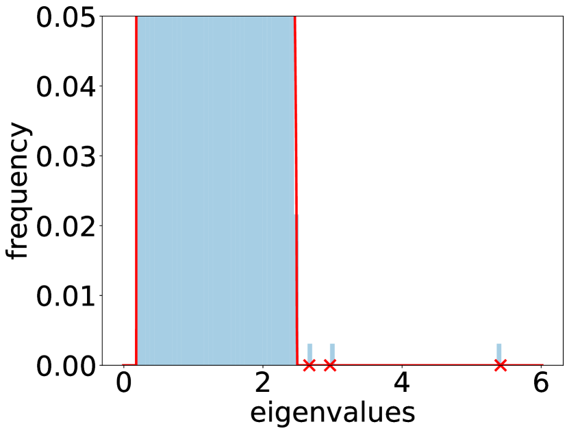
(a) Spectrum of $\boldsymbol{K}_{0}$

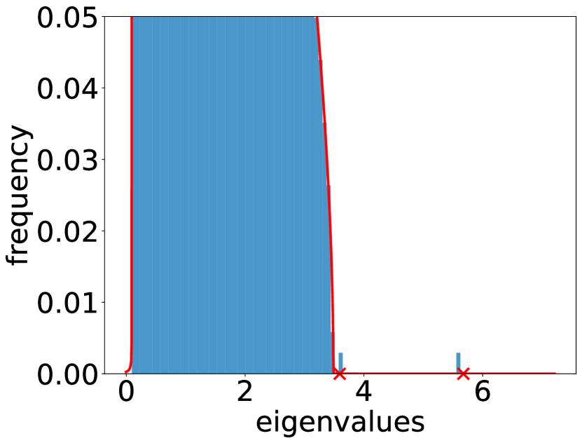
(b) Spectrum of $\boldsymbol{K}_{1}$

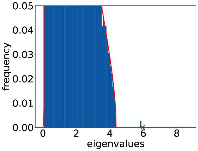
(c) Spectrum of $\boldsymbol{K}_{2}$

Figure 1: Spectra of three-layer CK matrices defined by (2.2) with $n=5000$, $d_{0}=d_{1}=d_{2}=15000$, and $\sigma\propto\arctan$. Input data is a GMM satisfying (2.9) with $r=3$, $\theta_{1}=2.0$, $\theta_{2}=1.18$, and $\theta_{3}=1.0$. (a)-(c) are theoretically predicted (red) and empirical (blue) bulk distributions and spikes of $\boldsymbol{K}_{\ell}$ for $\ell=0,1,2$.

Numerical illustration.

A simple illustration of this result for a 3-component Gaussian mixture model is provided in Figure 1. We note that $\mathcal{I}_{L}\subseteq\cdots\subseteq\mathcal{I}_{0}$ and $\varphi_{\ell}(s_{i,\ell-1})\in(0,1)$, so the number of spike eigenvalues of $\boldsymbol{K}_{\ell}$ induced by $\boldsymbol{K}_{0}$ and the alignment of the spike eigenvectors of $\boldsymbol{K}_{\ell}$ with the true class label vectors $\{\boldsymbol{b}_{i}\}_{i=1}^{r}$ are both non-increasing in the network depth, see also Figure 2. In other words, at random initialization, the input signal diminishes as the depth of the NN increases.

In Figure 2 we highlight two remedies to this “curse of depth” at random initialization.

• In Figure 2(a) we observe that when the width of NN becomes larger, alignment between the leading eigenvector of $\boldsymbol{K}_{\ell}$ at random initialization and the signal can be preserved across a larger depth. This illustrates the benefit of overparameterization by increasing the network width.

• In Figure 2(b) we observe that gradient descent training on the weight matrices also restores and even amplifies the informative signal in the CK matrix of each layer; specifically, after 50 steps of GD training (yellow curve), the alignment between the class labels and the leading eigenvector of $\boldsymbol{K}_{\ell}$ may increase through depth. This demonstrates the benefit of gradient-based feature learning. In Section 2.2 we precisely quantify this improved alignment due to gradient descent in a simplified two-layer setting.

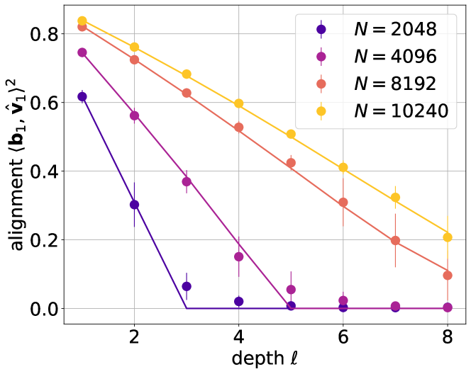
(a) Effect of width on alignment.

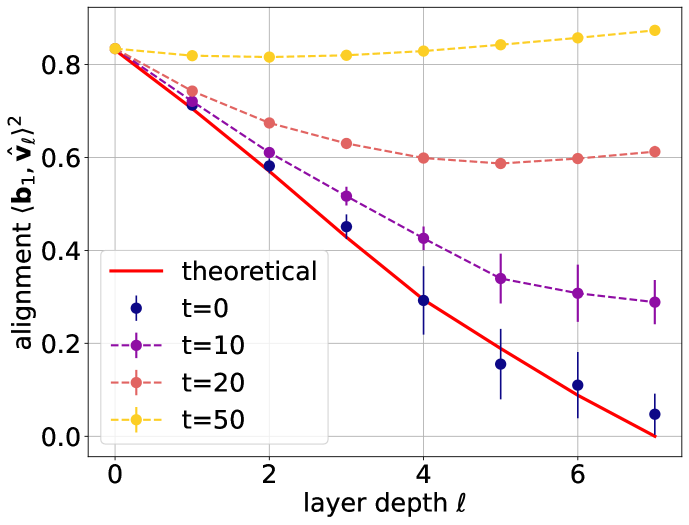
(b) Effect of GD training.

Figure 2: We consider multiple-layer NNs in (2.1) with $\sigma\propto\tanh$ on Gaussian mixture data (2.9) for $r=1$, and compute the alignment between the largest eigenvector of the CK matrix $\boldsymbol{K}_{\ell}$ with genuine signal $\boldsymbol{b}_{1}$ (class labels) for different layer $\ell$. (a) NNs at random initialization with varying hidden widths $N=2048,4096,8192,10240$. (b) NNs trained by gradient descent with learning rate $\eta=0.1$ for varying steps $T=0,10,20,50$; we use the $\mu$-parameterization [YH20] to encourage feature learning. $\theta_{1}$ is $2.5$ and $1.8$ for (a) and (b), respectively. Dots are empirical values (over 10 runs) and solid curves represent theoretical predictions at random initialization from Theorem 3.

2.2 CK matrix after $O(1)$ steps of gradient descent

The preceding section studied the spike eigenstructure of the CK induced by low-rank structure in the input data. Here, focusing on a two-layer model, we study an alternative setting where spiked structure arises instead in the weight matrix $\boldsymbol{W}$ from gradient descent training.

We consider an early training regime studied in [BES⁺22], with a width-$N$ two-layer feedforward NN,

$$f_{\text{NN}}(\boldsymbol{x})=\frac{1}{\sqrt{N}}\sum_{i=1}^{N}a_{i}\sigma(\langle\boldsymbol{x},\boldsymbol{w}_{i}\rangle)=\frac{1}{\sqrt{N}}\sigma(\boldsymbol{x}^{\top}\boldsymbol{W})\boldsymbol{a}.$$ (2.11)

Here $\boldsymbol{x}\in\mathbb{R}^{d}$ is the input, and $\boldsymbol{W}=[\boldsymbol{w}_{1},\ldots,\boldsymbol{w}_{N}]\in\mathbb{R}^{d\times N}$ and $\boldsymbol{a}\in\mathbb{R}^{N}$ are the network weights. For clarity of the subsequent discussion, we will transpose the notation for $\boldsymbol{X}$ and $\boldsymbol{W}$ from the preceding section, and incorporate a $1/\sqrt{d}$ scaling into $\boldsymbol{W}$ rather than into the input data $\boldsymbol{X}$.

Given are an input feature matrix $\boldsymbol{X}=[\boldsymbol{x}_{1},\ldots,\boldsymbol{x}_{n}]^{\top}\in\mathbb{R}^{n\times d}$ and labels $\boldsymbol{y}\in\mathbb{R}^{n}$ for $n$ samples, where $y_{i}=f_{*}(\boldsymbol{x}_{i})+\text{noise}$. We consider the training of first-layer weights $\boldsymbol{W}$ to minimize the mean squared error

$$\mathcal{L}(\boldsymbol{W})={\frac{1}{2n}}\sum_{i=1}^{n}(f_{\text{NN}}(\boldsymbol{x}_{i})-y_{i})^{2},$$

fixing the second-layer weight vector $\boldsymbol{a}$. From a random initialization $\boldsymbol{W}_{0}\in\mathbb{R}^{d\times N}$, and over $T$ steps with learning rates $\eta_{1},\ldots,\eta_{T}$ scaled by $\sqrt{N}$, the gradient descent (GD) updates take the form

$$\boldsymbol{W}_{\!t+1}=\boldsymbol{W}_{\!t}+\eta_{t+1}\sqrt{N}\cdot\boldsymbol{G}_{t},\qquad\boldsymbol{G}_{t}=-\nabla\mathcal{L}(\boldsymbol{W}_{t}).$$ (2.12)

Of interest is the information about the label function $f_{*}$ that is learned by $\boldsymbol{W}_{\text{trained}}\equiv\boldsymbol{W}_{T}$, which may be characterized by the spectral alignment of the CK matrix with the class label vector on independent test data $(\tilde{}\boldsymbol{X},\tilde{}\boldsymbol{y})$. This use of independent test data may be understood as a pre-training setup, also considered previously in [BES⁺22, MLHD23] and studied for real-world data in [WHS22].

It was shown in [BES⁺22] that in a training regime with initialization $\|\boldsymbol{W}_{0}\|\asymp 1$ such that $|f_{\text{NN}}(\boldsymbol{x}_{i})|\ll 1$ for each $i=1,\ldots,N$, and with learning rates $\eta_{1},\ldots,\eta_{T}\asymp 1$ for a fixed number $T$ of GD steps, the weight matrix $\boldsymbol{W}$ undergoes a change during training that is $O(1)$ in operator norm and approximately rank-1,

$$\boldsymbol{W}_{\text{trained}}\approx\boldsymbol{W}_{0}+\frac{\eta b_{\sigma}}{n}\boldsymbol{X}^{\top}\boldsymbol{y}\boldsymbol{a}^{\top}\qquad\text{ where }\qquad\eta=\sum_{t=1}^{T}\eta_{t}.$$

Moreover, [BES⁺22, Conjecture 4] conjectured that for the CK matrix

$$\boldsymbol{K}=\frac{1}{N}\sigma(\tilde{}\boldsymbol{X}\boldsymbol{W}_{\text{trained}})\sigma(\tilde{}\boldsymbol{X}\boldsymbol{W}_{\text{trained}})^{\top}\in\mathbb{R}^{n\times n}$$ (2.13)

defined by the pre-trained weights and test data $\tilde{}\boldsymbol{X}$, the resulting spike eigenvalue and the alignment of its spike eigenvector with the test labels $\tilde{}\boldsymbol{y}\in\mathbb{R}^{n}$ are accurately predicted by a Gaussian equivalent model. Our main result of this section is an affirmative verification of this conjecture and precise characterization of the spike eigenstructure of $\boldsymbol{K}$, in the following representative setting.

Assumption 4.

For a two-layer NN in (2.11) with GD training defined by (2.12), we assume that

1. $n,d,N\to\infty$ such that $N/d\to\gamma_{0}\in(0,\infty)$ and $N/n\to\gamma_{1}\in(0,\infty)$.

2. Training features $\boldsymbol{X}=[\boldsymbol{x}_{1},\ldots,\boldsymbol{x}_{n}]^{\top}\in\mathbb{R}^{n\times d}$ have entries $[\boldsymbol{X}]_{ij}\overset{iid}{\sim}\mathcal{N}(0,1)$, training labels $\boldsymbol{y}\in\mathbb{R}^{n}$ have entries $y_{i}=\sigma_{*}(\boldsymbol{\beta}_{*}^{\top}\boldsymbol{x}_{i})+\varepsilon_{i}$ where $\boldsymbol{\beta}_{*}\in\mathbb{R}^{d}$ is a deterministic unit vector and $\varepsilon_{i}\overset{iid}{\sim}\mathcal{N}(0,\sigma_{\varepsilon}^{2})$, and test data $(\tilde{}\boldsymbol{X},\tilde{}\boldsymbol{y})$ is an independent copy of $(\boldsymbol{X},\boldsymbol{y})$.

3. The NN activation $\sigma:\mathbb{R}\to\mathbb{R}$ and label function $\sigma_{*}:\mathbb{R}\to\mathbb{R}$ both satisfy Assumption 3, with $b_{\sigma}:=\mathbb{E}[\sigma^{\prime}(\xi)]\neq 0$ and $b_{\sigma_{*}}:=\mathbb{E}[\sigma_{*}^{\prime}(\xi)]\neq 0$.

4. The weight initializations satisfy $[\boldsymbol{W}_{0}]_{ij}\stackrel{{\scriptstyle\mathrm{\tiny{i.i.d.}}}}{{\sim}}\mathcal{N}(0,1/d)$ and $a_{j}\stackrel{{\scriptstyle\mathrm{\tiny{i.i.d.}}}}{{\sim}}\mathcal{N}(0,1/N)$.

5. The number of iterations $T$ and learning rates $\eta_{1},\ldots,\eta_{T}$ are fixed independently of $n,d,N$.

Under these assumptions, the following theorem characterizes the spike eigenvalue of the CK matrix and the alignment between the corresponding eigenvector and the test labels, as a function of the learning rate $\eta_{t}$ and the number of gradient descent steps $T$.

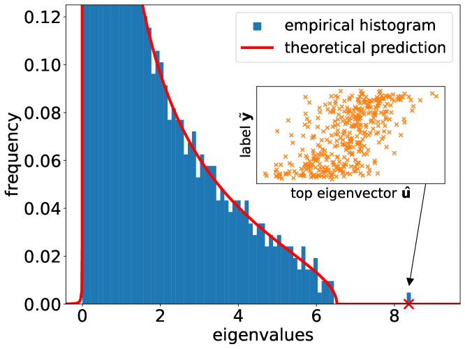
(a) Spectrum of the updated CK.

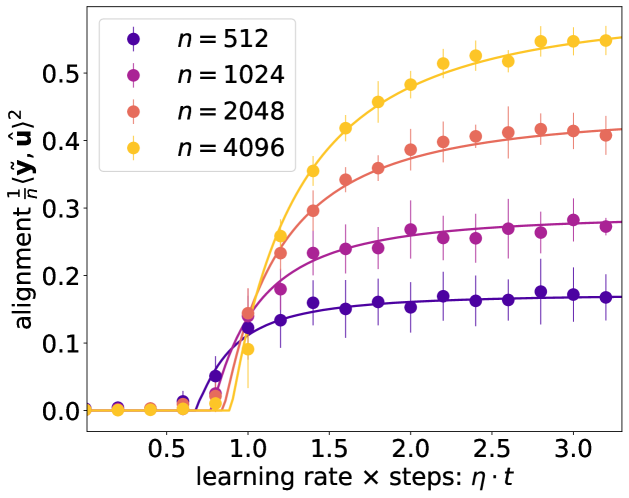
(b) Eigenvector alignment of the updated CK.

Figure 3: $(a)$ We set $n=2000,d=1600,N=2400,\eta\cdot t=2$, and $\sigma=\sigma_{*}=\text{erf}$. $(b)$ We set $d=2048,N=1024,\eta=0.2$, $\sigma=\text{tanh},\sigma_{*}=\text{SoftPlus}$, and vary the sample size $n$ and number of GD steps $t$; dots represent empirical simulations (over 10 runs) and solid curves are theoretical predictions from Theorem 5.

Theorem 5.

Suppose that Assumption 4 holds, and set $\eta=\sum_{t=1}^{T}\eta_{t}$. Define

$$\theta_{1}=b_{\sigma}\eta\cdot\sqrt{(\gamma_{1}/\gamma_{0})(1+\sigma_{\varepsilon}^{2})+b_{\sigma_{*}}^{2}},\qquad\theta_{2}=b_{\sigma}b_{\sigma_{*}}\eta.$$ (2.14)

Let $z_{1}(\cdot)$ and $\varphi_{1}(\cdot)$ be defined by (2.7) with $\gamma_{1}$ and $\nu_{0}=b_{\sigma}^{2}\otimes\rho^{\textnormal{MP}}_{\gamma_{0}}\oplus(1-b_{\sigma}^{2})$, and set

$$\lambda_{1}=b_{\sigma}^{2}\frac{(1+\theta_{1}^{2})(\gamma_{0}+\theta_{1}^{2})}{\theta_{1}^{2}}+1-b_{\sigma}^{2}.$$

Then $\boldsymbol{K}$ defined by (2.13) has a spike eigenvalue if and only if $\theta_{1}>\gamma_{0}^{1/4}$ and $z^{\prime}(-1/\lambda_{1})>0$. In this case, $\lambda_{\max}(\boldsymbol{K})\to\gamma_{1}^{-1}z(-1/\lambda_{1})$ a.s., and the leading unit eigenvector $\widehat{}\boldsymbol{u}\in\mathbb{R}^{n}$ of $\boldsymbol{K}$ satisfies

$$\frac{1}{\sqrt{n}}|\tilde{\boldsymbol{y}}^{\top}\widehat{}\boldsymbol{u}|\to b_{\sigma}b_{\sigma_{*}}\frac{\sqrt{z(-1/\lambda_{1})\varphi(-1/\lambda_{1})}}{\lambda_{1}}\cdot\frac{\theta_{2}\sqrt{(\theta_{1}^{4}-\gamma_{0})(\gamma_{0}+\theta_{1}^{2})}}{\theta_{1}^{3}}>0\text{ a.s.}$$ (2.15)

Numerical illustration.

Figure 3 empirically validates the predictions of Theorem 5, for a two-layer NN trained with a small number of GD steps. Figure 3(a) shows that one spike eigenvalue emerges over training in the test-data CK, the location of which is accurately predicted by Theorem 5; moreover, the leading eigenvector $\widehat{\boldsymbol{u}}$ aligns with the labels $\tilde{\boldsymbol{y}}$. This is quantified in Figure 3(b), where above a phase transition threshold, the alignment $\langle\widehat{\boldsymbol{u}},\tilde{\boldsymbol{y}}\rangle^{2}$ (predicted by (2.15)) increases with the learning rate or number of GD steps; in addition, alignment also increases with the training set size $n$. Compared with random initialization ($\eta=0$), this illustrates that training improves the NN representation, and the test-data CK contains information on the label function $f_{*}$.

3 Analysis of a nonlinear spiked covariance model

The results of Sections 2.1 and 2.2 rest on an analysis of spiked eigenstructure in a general nonlinear spiked covariance model. We describe the assumptions and statement of this general result informally here, deferring formal and more quantitative statements to Appendix B.

Let $\boldsymbol{G}=\frac{1}{\sqrt{N}}[\boldsymbol{g}_{1},\ldots,\boldsymbol{g}_{N}]^{\top}\in\mathbb{R}^{N\times n}$ have independent rows $\boldsymbol{g}_{1},\ldots,\boldsymbol{g}_{N}\in\mathbb{R}^{n}$ with mean 0 and common covariance $\boldsymbol{\Sigma}\in\mathbb{R}^{n\times n}$. We assume that the law of $\boldsymbol{g}_{i}$ satisfies concentration of quadratic forms $\boldsymbol{g}_{i}^{\top}\boldsymbol{A}\boldsymbol{g}_{j}$, but has otherwise arbitrary dependence across coordinates. As $n,N\to\infty$ with $n/N\to\gamma\in(0,\infty)$, the eigenvalues of $\boldsymbol{\Sigma}$ satisfy

$$\lambda_{i}(\boldsymbol{\Sigma})\to\lambda_{i}\text{ for }i=1,\ldots,r,\qquad\frac{1}{n-r}\sum_{i=r+1}^{n}\delta_{\lambda_{i}(\boldsymbol{\Sigma})}\to\nu\text{ weakly},$$

for fixed spike values $\lambda_{1},\ldots,\lambda_{r}>0$ and a deterministic limit spectral law $\nu$. Then the empirical spectral law of the sample covariance matrix $\boldsymbol{K}=\boldsymbol{G}^{\top}\boldsymbol{G}$ satisfies

$$\frac{1}{n}\sum_{i=1}^{n}\delta_{\lambda_{i}(\boldsymbol{K})}\to\mu=\rho_{\gamma}^{\textnormal{MP}}\boxtimes\nu\text{ weakly a.s.}$$

Under these assumptions, let us define

$$z(s)={-}\frac{1}{m}+\gamma\int\frac{\lambda}{1+\lambda s}d\nu(\lambda),\qquad\varphi(s)=\frac{z^{\prime}(s)}{(-1/s)z(s)}.$$

Theorem 6 (informal).

1. If $r=0$, then all eigenvalues of $\boldsymbol{K}$ converge to $\mathrm{supp}({\mu})\cup\{0\}$. More generally for $r\geq 0$, the eigenvalues of $\boldsymbol{K}$ asymptotically separated from $\mathrm{supp}({\mu})\cup\{0\}$ are in 1-to-1 correspondence with $\mathcal{I}=\{i:z^{\prime}(-1/\lambda_{i})>0\}$, and $\widehat{\lambda}_{i}(\boldsymbol{K})\to z(-1/\lambda_{i})$.

2. For each $i\in\mathcal{I}$ and any deterministic unit vector $\boldsymbol{v}\in\mathbb{R}^{n}$, $(\boldsymbol{v}^{\top}\widehat{}\boldsymbol{v}_{i})^{2}-\varphi(-1/\lambda_{i})(\boldsymbol{v}^{\top}\boldsymbol{v}_{i})^{2}\to 0$, where $\boldsymbol{v}_{i},\widehat{}\boldsymbol{v}_{i}$ are the unit eigenvectors of $\boldsymbol{\Sigma},\boldsymbol{K}$ for eigenvalues $\lambda_{i}(\boldsymbol{\Sigma}),\widehat{\lambda}_{i}(\boldsymbol{K})$.

3. Let $\boldsymbol{u}=\frac{1}{\sqrt{N}}(u_{1},\ldots,u_{N})^{\top}\in\mathbb{R}^{N}$ be such that $[\boldsymbol{u},\boldsymbol{G}]\in\mathbb{R}^{N\times(n+1)}$ has i.i.d. rows $\{[u_{j},\boldsymbol{g}_{j}]\}_{j=1}^{N}$, and denote $\mathbb{E}[u\boldsymbol{g}]=\mathbb{E}[u_{j}\boldsymbol{g}_{j}]$ for all $j\in[N]$. Then for each $i\in\mathcal{I}$,

   $$(\boldsymbol{u}^{\top}\widehat{\boldsymbol{u}}_{i})^{2}-\frac{z(-1/\lambda_{i})\varphi(-1/\lambda_{i})}{\lambda_{i}^{2}}(\mathbb{E}[u\boldsymbol{g}]^{\top}\boldsymbol{v}_{i})^{2}\to 0$$

   where $\widehat{\boldsymbol{u}}_{i}$ is the unit eigenvector of $\boldsymbol{G}\boldsymbol{G}^{\top}$ for its eigenvalue $\widehat{\lambda}_{i}(\boldsymbol{G}\boldsymbol{G}^{\top})=\widehat{\lambda}_{i}(\boldsymbol{K})$.

Statements (a–b) are known in a linear setting $\boldsymbol{g}_{i}=\boldsymbol{\Sigma}^{1/2}\boldsymbol{z}_{i}$ when $\boldsymbol{z}_{i}$ has i.i.d. entries, see e.g. [BY12] and [YZB15, Theorems 11.3 and 11.5]. The above theorem thus verifies an exact asymptotic equivalence between spiked spectral phenomena in a nonlinear spiked covariance model with those of a linearly defined (possibly Gaussian) model.

In Section 2.1, each CK matrix $\boldsymbol{K}_{\ell}$ has (approximately) the structure of the above matrix $\boldsymbol{K}$ over the randomness of $\boldsymbol{W}_{\ell}$, conditional on the features $\boldsymbol{X}_{\ell-1}$ of the preceding layer, and Theorem 3 follows from Theorem 6(a,b). In Section 2.2, the CK matrix $\boldsymbol{K}$ defined by trained weights has (approximately) this structure over the randomness of $\tilde{}\boldsymbol{X}$, conditional on $\boldsymbol{W}_{\mathrm{trained}}$, and Theorem 5 follows from Theorem 6(a,c).

Proof ideas.

Analyses in the linearly defined model $\boldsymbol{g}_{i}=\boldsymbol{\Sigma}^{1/2}\boldsymbol{z}_{i}$ commonly stem from block matrix inversion identities with respect to the block decompositions

$$\boldsymbol{\Sigma}=\begin{pmatrix}\boldsymbol{\Sigma}_{r}&\mathbf{0}\\ \mathbf{0}&\boldsymbol{\Sigma}_{0}\end{pmatrix},\qquad\boldsymbol{G}=\begin{pmatrix}\boldsymbol{G}_{r}&\boldsymbol{G}_{0}\end{pmatrix}$$

where $\boldsymbol{\Sigma}_{r}$ contains the spike eigenvalues of $\boldsymbol{\Sigma}$, and $\boldsymbol{G}_{r}$ is independent of $\boldsymbol{G}_{0}$. This independence does not hold in our setting, and we develop a different “master equation” approach.

Let $\widehat{\lambda}^{1/2}$ be a spike singular value of $\boldsymbol{G}$ with corresponding unit singular vectors $(\widehat{}\boldsymbol{u},\widehat{}\boldsymbol{v})$. We consider the linearized equation

$$0=\begin{pmatrix}-\widehat{\lambda}\boldsymbol{I}&\boldsymbol{G}^{\top}\\ \boldsymbol{G}&-\boldsymbol{I}\end{pmatrix}\begin{pmatrix}\widehat{}\boldsymbol{v}\\ \widehat{\lambda}^{1/2}\widehat{}\boldsymbol{u}\end{pmatrix}.$$ (3.1)

Writing $\boldsymbol{V}_{r}\in\mathbb{R}^{n\times r}$ for the $r$ spike eigenvectors of $\boldsymbol{\Sigma}$, we define a generalized resolvent

$$\boldsymbol{\mathcal{R}}(z,\alpha)=\begin{pmatrix}-z\boldsymbol{I}-\alpha\boldsymbol{V}_{r}\boldsymbol{V}_{r}^{\top}&\boldsymbol{G}^{\top}\\ \boldsymbol{G}&-\boldsymbol{I}\end{pmatrix}^{-1},$$

add to (3.1) the quantity $-\alpha\begin{pmatrix}\boldsymbol{V}_{r}\\ \mathbf{0}\end{pmatrix}\cdot\boldsymbol{V}_{r}^{\top}\widehat{}\boldsymbol{v}$ on both sides for some large $\alpha>0$, and rewrite this as

$$\begin{pmatrix}\widehat{}\boldsymbol{v}\\ \widehat{\lambda}^{1/2}\widehat{}\boldsymbol{u}\end{pmatrix}=-\alpha\,\boldsymbol{\mathcal{R}}(\widehat{\lambda},\alpha)\begin{pmatrix}\boldsymbol{V}_{r}\\ \mathbf{0}\end{pmatrix}\cdot\boldsymbol{V}_{r}^{\top}\widehat{}\boldsymbol{v}.$$ (3.2)

We will show that $\boldsymbol{\mathcal{R}}(z,\alpha)$ exists and is bounded in operator norm for any $z$ separated from the limit bulk spectral support of $\boldsymbol{K}$ and any large enough $\alpha>0$. Then, multiplying (3.2) by $(\boldsymbol{V}_{r}^{\top}\;\mathbf{0})$ and applying a block matrix inversion identity,

$$\boldsymbol{V}_{r}^{\top}\widehat{}\boldsymbol{v} ={-}\alpha\begin{pmatrix}\boldsymbol{V}_{r}\\ \mathbf{0}\end{pmatrix}^{\top}\boldsymbol{\mathcal{R}}(\widehat{\lambda},\alpha)\begin{pmatrix}\boldsymbol{V}_{r}\\ \mathbf{0}\end{pmatrix}\cdot\boldsymbol{V}_{r}^{\top}\widehat{}\boldsymbol{v}=-\alpha\boldsymbol{V}_{r}^{\top}\Big{(}\boldsymbol{G}^{\top}\boldsymbol{G}-\widehat{\lambda}\boldsymbol{I}-\alpha\boldsymbol{V}_{r}\boldsymbol{V}_{r}^{\top}\Big{)}^{-1}\boldsymbol{V}_{r}\cdot\boldsymbol{V}_{r}^{\top}\widehat{}\boldsymbol{v}.$$

As a result, spike eigenvalues $\widehat{\lambda}$ are roots $z=\widehat{\lambda}$ of the master equation

$$\det\mathopen{}\mathclose{{}\left(\boldsymbol{I}_{r}+\alpha\boldsymbol{V}_{r}^{\top}\Big{(}\boldsymbol{G}^{\top}\boldsymbol{G}-z\boldsymbol{I}-\alpha\boldsymbol{V}_{r}\boldsymbol{V}_{r}^{\top}\Big{)}^{-1}\boldsymbol{V}_{r}}\right)=0,$$

for any fixed and large $\alpha>0$. Singular vector alignments may be characterized likewise from (3.2).

The core of the proof is an asymptotic analysis of this master equation via a deterministic equivalent approximation

$$\boldsymbol{v}_{1}^{\top}\boldsymbol{R}(\boldsymbol{\Gamma})\boldsymbol{v}_{2}:=\boldsymbol{v}_{1}^{\top}(\boldsymbol{G}^{\top}\boldsymbol{G}-\boldsymbol{\Gamma})^{-1}\boldsymbol{v}_{2}\approx{-}\boldsymbol{v}_{1}^{\top}(\boldsymbol{\Gamma}+z\tilde{m}(z)\boldsymbol{\Sigma})^{-1}\boldsymbol{v}_{2}$$ (3.3)

for any deterministic unit vectors $\boldsymbol{v}_{1},\boldsymbol{v}_{2}\in\mathbb{R}^{n}$ and low-rank perturbations $\boldsymbol{\Gamma}$ of $z\boldsymbol{I}$, where $\tilde{m}(z)$ is the Stieltjes transform of the “companion” limit measure $\tilde{\mu}$ for the eigenvalue distribution of $\boldsymbol{G}\boldsymbol{G}^{\top}\in\mathbb{R}^{N\times N}$. We extend results of [Cho22, SCDL23] by establishing this approximation not only for $\boldsymbol{\Gamma}=z\boldsymbol{I}$ but also perturbations thereof, and for spectral arguments $z\in\mathbb{C}\setminus\mathrm{supp}({\mu})$ that may belong to the positive real line. The latter extension requires showing, a priori, that all eigenvalues of $\boldsymbol{K}=\boldsymbol{G}^{\top}\boldsymbol{G}$ fall close to $\mathrm{supp}({\mu})$ in the absence of spiked structure. We show this by adapting an argument of [BS98] and using a fluctuation averaging lemma described below.

Let us conclude with a brief discussion of our proof of (3.3): From manipulations of the identity

$$\operatorname{Tr}\boldsymbol{B}=\operatorname{Tr}(\boldsymbol{G}^{\top}\boldsymbol{G}-\boldsymbol{\Gamma})\boldsymbol{R}(\boldsymbol{\Gamma})\boldsymbol{B}={-}\operatorname{Tr}\boldsymbol{R}(\boldsymbol{\Gamma})\boldsymbol{B}\boldsymbol{\Gamma}+\frac{1}{N}\sum_{i=1}^{N}\boldsymbol{g}_{i}^{\top}\boldsymbol{R}(\boldsymbol{\Gamma})\boldsymbol{B}\boldsymbol{g}_{i}$$

for appropriately chosen matrices $\boldsymbol{B}\in\mathbb{C}^{n\times n}$, the Sherman-Morrison (leave-one-out) formula for matrix inversion applied to $\boldsymbol{R}(\boldsymbol{\Gamma})$, and the concentration of bilinear forms in $\boldsymbol{g}_{i}$, one may show

$$\boldsymbol{v}_{1}^{\top}(\boldsymbol{\Gamma}+z\tilde{m}(z)\boldsymbol{\Sigma})^{-1}\boldsymbol{v}_{2}\approx{-}\boldsymbol{v}_{1}^{\top}\boldsymbol{R}(\boldsymbol{\Gamma})\boldsymbol{v}_{2}+\frac{1}{1+N^{-1}\operatorname{Tr}\boldsymbol{\Sigma}\boldsymbol{R}(\boldsymbol{\Gamma})}\cdot\frac{1}{N}\sum_{i=1}^{N}(1-\mathbb{E}_{\boldsymbol{g}_{i}})T_{i}$$ (3.4)

where $T_{i}=\boldsymbol{g}_{i}^{\top}\boldsymbol{R}^{(i)}(\boldsymbol{\Gamma})\boldsymbol{v}_{2}\cdot\boldsymbol{v}_{1}^{\top}(\boldsymbol{\Gamma}+zm_{\tilde{}\boldsymbol{K}}^{(i)}(\boldsymbol{\Gamma})\boldsymbol{\Sigma})^{-1}\boldsymbol{g}_{i}$. Here, $\boldsymbol{R}^{(i)}(\boldsymbol{\Gamma})$ and $m_{\tilde{}\boldsymbol{K}}^{(i)}(\boldsymbol{\Gamma})$ are generalized leave-one-out resolvents and empirical Stieltjes transforms defined by $\{\boldsymbol{g}_{j}\}_{j\neq i}$, and $\mathbb{E}_{\boldsymbol{g}_{i}}$ is the partial expectation over only $\boldsymbol{g}_{i}$. Under our assumptions for $\boldsymbol{g}_{i}$, each error term $(1-\mathbb{E}_{\boldsymbol{g}_{i}})T_{i}$ has mean 0 and $O(1)$ fluctuations. We develop a fluctuation averaging lemma using recursive applications of the Sherman-Morrison identity to further resolve the dependence of $\boldsymbol{R}^{(i)}(\boldsymbol{\Gamma})$ and $m_{\tilde{}\boldsymbol{K}}^{(i)}(\boldsymbol{\Gamma})$ on fixed subsets of rows $\{\boldsymbol{g}_{j}\}_{j\neq i}$, to show that the errors $(1-\mathbb{E}_{\boldsymbol{g}_{i}})T_{i}$ are weakly correlated across $i\in[N]$. Hence their average has a mean 0 and fluctuates on the asymptotically negligible scale of $O(N^{-1/2})$, and applying this to (3.4) shows (3.3).

Acknowledgements

This research was supported in part by NSF DMS-2142476, NSF DMS-2055340 and NSF DMS-2154099.

Organization of the Appendices

• Appendix A introduces relevant notation and background.

• Appendix B states our main results for the general nonlinear spiked covariance model

  $$\boldsymbol{K}=\boldsymbol{G}^{\top}\boldsymbol{G},$$

  formalizing the discussion in Section 3. These results are divided into two subsections: Appendix B.1 gives a “no outliers” statement for $\boldsymbol{K}$ and a deterministic equivalent approximation for its resolvent, under minimal asymptotic assumptions. Appendix B.2 then states the main characterizations of spike eigenvalues/eigenvectors in an asymptotic setting with a spiked eigenstructure.

• Appendix C develops a general fluctuation averaging lemma for the sample covariance model, and proves the results of Appendix B.1.

• Appendix D proves the results of Appendix B.2.

• Finally, Appendix E proves the results of Section 2.1 on propagation of spiked eigenstructure through the layers of a neural network, and Appendix F proves the results of Section 2.2 on the eigenstructure of the CK after gradient descent training.

Appendix A Notations and background

A.1 Stochastic domination

We use the following standard notation for stochastic domination of random variables, see e.g. [EKY13, Definition 2.4]: For random variables $X\equiv X(u)$ and $Y\equiv Y(u)\geq 0$ depending implicitly on $N$ and a parameter $u\in U_{N}$, as $N\to\infty$, we write

$$X\prec Y\text{ or }X=O_{\prec}\mathopen{}\mathclose{{}\left(Y}\right)\text{ uniformly over }u\in U_{N}$$

if, for any fixed $\varepsilon,D>0$ and all large $N$,

$$\sup_{u\in U_{N}}\mathbb{P}\Big{[}|X(u)|>N^{\varepsilon}Y(u)\Big{]}<N^{-D}.$$

Throughout, “for all large $N$” means for all $N\geq N_{0}$ where $N_{0}$ may depend on $\varepsilon,D$, any quantities that are constant in the context of the statement, and convergence rates of the spike eigenvalues and empirical spectral measures in the given assumptions.

If $X=\mathbf{1}\{\mathcal{E}\}$ is the indicator of an event $\mathcal{E}\equiv\mathcal{E}_{N}$, then $\mathbf{1}\{\mathcal{E}\}\prec 0$ means $\mathbb{P}[\mathcal{E}]<N^{-D}$ for any fixed $D>0$ and all large $N$. If $X$ and $Y$ are both deterministic, then $X\prec Y$ means $|X|\leq N^{\varepsilon}Y$ (deterministically) for any $\varepsilon>0$ and all large $N$. For an event $\mathcal{E}\equiv\mathcal{E}_{N}$, we will write

$$X=O_{\prec}^{\,\mathcal{E}}\mathopen{}\mathclose{{}\left(Y}\right)$$

as shorthand for $X\cdot\mathbf{1}\{\mathcal{E}\}\prec Y$.

We will use the following basic properties often implicitly.

Proposition 7.

Suppose $X\prec Y$ uniformly over $u\in U_{N}$.

1. If $|U_{N}|\leq N^{C}$ for a constant $C>0$, then for any fixed $\varepsilon,D>0$ and all large $N$,

   $$\mathbb{P}\Big{[}\text{there exists }u\in U_{N}\text{ with }|X(u)|\geq N^{\varepsilon}Y(u)\Big{]}\leq N^{-D}.$$

2. If $|U_{N}|\leq N^{C}$ for a constant $C>0$, then $\sum_{u\in U_{N}}X(u)\prec\sum_{u\in U_{N}}Y(u)$.

3. If $|U_{N}|\leq C$ for a constant $C>0$, then $\prod_{u\in U_{N}}X(u)\prec\prod_{u\in U_{N}}Y(u)$.

4. If $Y$ is deterministic, and $\mathbb{E}[X^{2}]\leq N^{C}$ and $Y\geq N^{-C}$ for a constant $C>0$, then also $\mathbb{E}[|X|]\prec Y$ uniformly over $u\in U_{N}$.

Proof.  The first three statements follow from a union bound over $U_{N}$. For the last statement, for any fixed $\varepsilon>0$, observe that

$$\mathbb{E}|X|\leq N^{\varepsilon/2}Y+\mathbb{E}\Big{[}|X|\mathbf{1}\{|X|>N^{\varepsilon/2}Y\}\Big{]}\leq N^{\varepsilon/2}Y+\mathbb{E}[X^{2}]^{1/2}\mathbb{P}[|X|>N^{\varepsilon/2}Y]^{1/2}.$$

Applying $\mathbb{E}[X^{2}]\leq N^{C}$, $Y\geq N^{-C}$, and $\mathbb{P}[|X|>N^{\varepsilon/2}Y]<N^{-D}$ for sufficiently large $D>0$ shows that the second term is less than $N^{\varepsilon/2}Y$ for all large $N$, hence $\mathbb{E}|X|<N^{\varepsilon}Y$. ∎

A.2 Deformed Marcenko-Pastur law

For a probability measure $\nu$ supported on $[0,\infty)$ and an aspect ratio parameter $\gamma>0$, consider the deformed Marcenko–Pastur measure

$$\mu=\rho^{\textnormal{MP}}_{\gamma}\boxtimes\nu$$

and its “companion” probability measure

$$\tilde{\mu}=\gamma\mu+(1-\gamma)\delta_{0}.$$

Here, $\mu$ and $\tilde{\mu}$ represent the limit eigenvalue distributions of $\boldsymbol{G}^{\top}\boldsymbol{G}\in\mathbb{R}^{n\times n}$ and $\boldsymbol{G}\boldsymbol{G}^{\top}\in\mathbb{R}^{N\times N}$ respectively, when $\boldsymbol{G}=\frac{1}{\sqrt{N}}[\boldsymbol{g}_{1},\ldots,\boldsymbol{g}_{N}]\in\mathbb{R}^{N\times n}$ has i.i.d. rows with mean 0 and covariance $\boldsymbol{\Sigma}$, and $n,N\to\infty$ with $n/N\to\gamma$ and $\frac{1}{n}\sum_{i=1}^{n}\delta_{\lambda_{i}(\boldsymbol{\Sigma})}\to\nu$ weakly.

These measures $\mu,\tilde{\mu}$ may be defined by their Stieltjes transform

$$m(z)=\int\frac{1}{x-z}d\mu(x),\qquad\tilde{m}(z)=\int\frac{1}{x-z}d\tilde{\mu}(x)$$ (A.1)

where $\tilde{m}(z)=\gamma m(z)+(1-\gamma)(-1/z)$. By the results of [MP67, SB95], for any $z\in\mathbb{C}^{+}$, $m(z)$ and $\tilde{m}(z)$ are the unique roots in $\{m\in\mathbb{C}:\gamma m+(1-\gamma)(-1/z)\in\mathbb{C}^{+}\}$ and $\mathbb{C}^{+}$, respectively, to the Marcenko-Pastur equations

$$m(z)=\int\frac{1}{\lambda(1-\gamma-\gamma zm(z))-z}\,d\nu(\lambda),\quad z=-\frac{1}{\tilde{m}(z)}+\gamma\int\frac{\lambda}{1+\lambda\tilde{m}(z)}d\nu(\lambda).$$ (A.2)

We define $m(z),\tilde{m}(z)$ via (A.1) also on the full domains $\mathbb{C}\setminus\mathrm{supp}({\mu})$ and $\mathbb{C}\setminus\mathrm{supp}({\tilde{\mu}})$ respectively, where the support sets $\mathrm{supp}({\mu})$ and $\mathrm{supp}({\tilde{\mu}})$ may differ only at the single point $\{0\}$.

In the setting $\boldsymbol{\Sigma}=\boldsymbol{I}$ (and $\nu=\delta_{1}$), the law $\mu=\rho_{\gamma}^{\textnormal{MP}}$ is the standard Marcenko-Pastur law, with explicit density function with respect to Lebesgue measure

$$d\rho_{\gamma}^{\textnormal{MP}}(\lambda)=\frac{1}{2\pi}\frac{\sqrt{(\lambda_{+}-\lambda)(\lambda-\lambda_{-})}}{\gamma\lambda}\cdot\mathbf{1}_{\lambda\in[\lambda_{-},\lambda_{+}]}\,d\lambda,\qquad\lambda_{\pm}:=(1\pm\sqrt{\gamma})^{2}$$

for $\gamma\leq 1$, and an additional point mass $(1-1/\gamma)$ at 0 when $\gamma>1$.

In general, $\mu$ and $\tilde{\mu}$ do not have analytically explicit densities. However, $\mathrm{supp}({\tilde{\mu}})$ is explicitly characterized in [SC95], and we review this characterization here: Define

$$\mathcal{T}=\{0\}\cup\{-1/\lambda:\lambda\in\mathrm{supp}({\nu})\}.$$ (A.3)

For $\tilde{m}\in\mathbb{C}\setminus\mathcal{T}$, define

$$z(\tilde{m})={-}\frac{1}{\tilde{m}}+\gamma\int\frac{\lambda}{1+\lambda\tilde{m}}d\nu(\lambda).$$ (A.4)

In light of the second equation of (A.2), this may be understood as a formal inverse of $\tilde{m}(z)$. From [SC95, Theorems 4.1 and 4.2], we have the following properties.

Proposition 8.

$\tilde{m}(\cdot)$ defines a bijection from $\{z\in\mathbb{R}\setminus\mathrm{supp}({\tilde{\mu}})\}$ to $\{\tilde{m}\in\mathbb{R}\setminus\mathcal{T}:z^{\prime}(\tilde{m})>0\}$, whose inverse function is $z(\cdot)$. In particular, $x\in\mathbb{R}$ does not belong to $\mathrm{supp}({\tilde{\mu}})$ if and only if there exists $\tilde{m}\in\mathbb{R}\setminus\mathcal{T}$ such that $z^{\prime}(\tilde{m})>0$ and $z(\tilde{m})=x$.

A.3 Additional notation

For a probability measure $\mu$, its support is the closed set

$$\mathrm{supp}({\mu})=\{x\in\mathbb{R}:\mu(O)>0\text{ for any open neighborhood }O\ni x\}.$$

We write $\textnormal{dist}(x,A)=\inf\{|x-y|:y\in A\}$ and define the $\varepsilon$-neighborhood

$$\mathrm{supp}({\mu})+(-\varepsilon,\varepsilon)=\{x\in\mathbb{R}:\textnormal{dist}(x,\mathrm{supp}({\mu}))<\varepsilon\}.$$

We write $\delta_{x}$ for the probability measure given by a point mass at $x\in\mathbb{R}$, $a\mu_{0}+(1-a)\mu_{1}$ for the convex combination of $\mu_{0},\mu_{1}$, and $a\otimes\mu\oplus b$ for the law of $a\mathsf{x}+b$ when $\mathsf{x}\sim\mu$.

For vectors, $\|\boldsymbol{v}\|\equiv\|\boldsymbol{v}\|_{2}$ is the Euclidean norm. For matrices, $\|\boldsymbol{M}\|$ is the operator norm $\sup_{\boldsymbol{v}:\|\boldsymbol{v}\|=1}\|\boldsymbol{M}\boldsymbol{v}\|$, $\|\boldsymbol{M}\|_{F}$ is the Frobenius norm $(\operatorname{Tr}\boldsymbol{M}^{\top}\boldsymbol{M})^{1/2}$, $\operatorname{Tr}$ is the (unnormalized) matrix trace, and $\boldsymbol{A}\odot\boldsymbol{B}$ is the entrywise (Hadamard) product. We write $\mathop{\mathrm{missing}}{diag}(\boldsymbol{v})$ for the diagonal matrix with vector $\boldsymbol{v}$ along the main diagonal, and $\boldsymbol{I}_{n}$ for the $n\times n$ identity matrix.

Appendix B Results for the nonlinear spiked covariance model

B.1 Deterministic equivalent for the resolvent

We consider the sample covariance and Gram matrix

$$\boldsymbol{K}=\boldsymbol{G}^{\top}\boldsymbol{G}\in\mathbb{R}^{n\times n},\quad\widetilde{}\boldsymbol{K}=\boldsymbol{G}\boldsymbol{G}^{\top}\in\mathbb{R}^{N\times N},\quad\text{ where }\quad\boldsymbol{G}=\frac{1}{\sqrt{N}}[\boldsymbol{g}_{1},\ldots,\boldsymbol{g}_{N}]\in\mathbb{R}^{N\times n}.$$

The following are our basic assumptions, where we recall that $\mathbf{1}\{\mathcal{E}\}\prec 0$ means $\mathbb{P}[\mathcal{E}]\leq N^{-D}$ for any fixed $D>0$ and all large $N$.

Assumption 5.

The rows of $\boldsymbol{G}$ are independent and satisfy $\mathbb{E}[\boldsymbol{g}_{i}]=\mathbf{0}$ and $\mathbb{E}[\boldsymbol{g}_{i}\boldsymbol{g}_{i}^{\top}]=\boldsymbol{\Sigma}$ for all $i\in[N]$, such that:

1. There exist constants $C,c>0$ such that $c<n/N<C$ and $\|\boldsymbol{\Sigma}\|<C$.

2. There exists a constant $B>0$ such that $\mathbf{1}\{\|\boldsymbol{K}\|>B\}\prec 0$.

3. Uniformly over deterministic matrices $\boldsymbol{A}\in\mathbb{C}^{n\times n}$ and over $i\neq j\in[N]$,

   $$\boldsymbol{g}_{i}^{\top}\boldsymbol{A}\boldsymbol{g}_{i}-\mathbb{E}[\boldsymbol{g}_{i}^{\top}\boldsymbol{A}\boldsymbol{g}_{i}]\prec\|\boldsymbol{A}\|_{F},\qquad\boldsymbol{g}_{i}^{\top}\boldsymbol{A}\boldsymbol{g}_{j}\prec\|\boldsymbol{A}\|_{F}.$$

4. For any integer $\alpha>0$, there exists a constant $C=C(\alpha)>0$ such that $\mathbb{E}[\|\boldsymbol{g}_{i}\|^{\alpha}]\leq N^{C}$.

Denote the finite-$N$ dimension ratio and empirical eigenvalue distribution of $\boldsymbol{\Sigma}$ by

$$\gamma_{N}=\frac{n}{N},\qquad\nu_{N}=\frac{1}{n}\sum_{i=1}^{n}\delta_{\lambda_{i}(\boldsymbol{\Sigma})}.$$ (B.1)

Let

$$\mu_{N}=\rho_{\gamma_{N}}^{\textnormal{MP}}\boxtimes\nu_{N},\qquad\tilde{\mu}_{N}=\gamma_{N}\mu_{N}+(1-\gamma_{N})\delta_{0}.$$

Denote the Stieltjes transforms of $\mu_{N},\tilde{\mu}_{N}$ by $m_{N}(z),\tilde{m}_{N}(z)$. These are characterized exactly as in (A.2) with $(\gamma_{N},\nu_{N})$ in place of $(\gamma,\nu)$.

We first establish that with high probability, $\boldsymbol{K}$ and $\widetilde{}\boldsymbol{K}$ have no outlier eigenvalues far from the support set

$$\mathcal{S}_{N}=\mathrm{supp}({\mu_{N}})\cup\{0\}=\mathrm{supp}({\tilde{\mu}_{N}})\cup\{0\}.$$ (B.2)

Theorem 9.

Suppose Assumption 5 holds. Then for any fixed $\varepsilon>0$,

$$\mathbf{1}\Big{\{}\boldsymbol{K}\text{ has an eigenvalue outside }\mathcal{S}_{N}+(-\varepsilon,\varepsilon)\Big{\}}\prec 0.$$

In asymptotic settings where $\nu_{N}\to\nu$ and $\mu_{N}\to\mu$ weakly and $\boldsymbol{\Sigma}$ has no spike eigenvalues, this set $\mathcal{S}_{N}$ will converge to $\mathcal{S}:=\mathrm{supp}({\mu})\cup\{0\}$. In general, $\mathcal{S}_{N}$ may contain intervals around spike eigenvalues of $\boldsymbol{K}$ that are separated from $\mathrm{supp}({\mu})\cup\{0\}$ if $\boldsymbol{\Sigma}$ has a spiked structure, and this will be clarified in the subsequent section.

Next, we establish a deterministic equivalent approximation for the resolvent of $\boldsymbol{K}$, for spectral arguments separated from this support set $\mathcal{S}_{N}$. Let us denote by

$$\boldsymbol{R}(z)=(\boldsymbol{K}-z\boldsymbol{I})^{-1},\qquad m_{\boldsymbol{K}}(z)=\frac{1}{n}\operatorname{Tr}\boldsymbol{R}(z)$$

the resolvent and Stieltjes transform of $\boldsymbol{K}$ for $z\not\in\mathrm{supp}({\mu_{N}})$. For any $\varepsilon>0$, define the domain

$$U_{N}(\varepsilon)=\Big{\{}z\in\mathbb{C}:\,|z|\leq\varepsilon^{-1},\,\textnormal{dist}(z,\mathcal{S}_{N})\geq\varepsilon\Big{\}}.$$ (B.3)

Theorem 10.

Suppose Assumption 5 holds. Then for any fixed $\varepsilon>0$, uniformly over $z\in U_{N}(\varepsilon)$ and over deterministic matrices $\boldsymbol{A}\in\mathbb{C}^{n\times n}$, we have

$$m_{\boldsymbol{K}}(z)-m_{N}(z)\prec\frac{1}{N},\qquad\operatorname{Tr}\Big{[}\boldsymbol{R}(z)\boldsymbol{A}-(-z\tilde{m}_{N}(z)\boldsymbol{\Sigma}-z\boldsymbol{I})^{-1}\boldsymbol{A}\Big{]}\prec\frac{1}{\sqrt{N}}\,\|\boldsymbol{A}\|_{F}.$$

For spectral arguments $z\in\mathbb{C}\setminus\mathbb{R}_{+}$ separated from the positive real line, such a result has been shown recently in [Cho22, SCDL23] (using different proof techniques). We use Theorem 9 as an input to establish this approximation also for spectral arguments in $\mathbb{R}_{+}\setminus\mathcal{S}_{N}$, as such a result (and its extension to a generalized resolvent) is needed for our analysis of spiked eigenstructure to follow.

B.2 Spike eigenvalues and eigenvectors

Now we consider an asymptotic setting with a specific spiked structure for the population covariance matrix $\boldsymbol{\Sigma}$, having a fixed number of spikes outside the support of the weak limit of its spectral law. This assumption is summarized as follows.

Assumption 6.

$\boldsymbol{\Sigma}$ has eigenvalues $\lambda_{1}(\boldsymbol{\Sigma}),\ldots,\lambda_{n}(\boldsymbol{\Sigma})$ (not necessarily ordered by magnitude) where, for a fixed integer $r\geq 0$, as $N\to\infty$:

1. $n/N\to\gamma\in(0,\infty)$.

2. There exists a probability measure $\nu$ with compact support in $(0,\infty)$, such that

   $$\frac{1}{n-r}\sum_{i=r+1}^{n}\delta_{\lambda_{i}(\boldsymbol{\Sigma})}\to\nu\text{ weakly.}$$

   Furthermore, for any fixed $\varepsilon>0$ and all large $N$,

   $$\lambda_{i}(\boldsymbol{\Sigma})\in\mathrm{supp}({\nu})+(-\varepsilon,\varepsilon)\text{ for all }i\geq r+1.$$

3. There exist distinct values $\lambda_{1},\ldots,\lambda_{r}>0$ with $\lambda_{1},\ldots,\lambda_{r}\not\in\mathrm{supp}({\nu})$ such that

   $$\lambda_{i}(\boldsymbol{\Sigma})\to\lambda_{i}\text{ for all }i=1,\ldots,r.$$

Under this assumption, we analyze the outlier singular values of $\boldsymbol{G}$ and their corresponding singular vectors. Let

$$\gamma_{N,0}=\frac{n-r}{N},\qquad\nu_{N,0}=\frac{1}{n-r}\sum_{i=r+1}^{n}\delta_{\lambda_{i}(\boldsymbol{\Sigma})}$$

be the finite-$N$ aspect ratio and population spectral measure corresponding to the bulk component of $\boldsymbol{\Sigma}$. Define the laws

$$\mu_{N,0}=\rho_{\gamma_{N,0}}^{\textnormal{MP}}\boxtimes\nu_{N,0},\qquad\tilde{\mu}_{N,0}=\gamma_{N,0}\mu_{N,0}+(1-\gamma_{N,0})\delta_{0}$$

and let $m_{N,0}(z),\tilde{m}_{N,0}(z)$ be their Stieltjes transforms. In the setting of Assumption 6, we note that $\mu_{N,0}\to\mu=\rho_{\gamma}^{\textnormal{MP}}\boxtimes\nu$ and $\tilde{\mu}_{N,0}\to\tilde{\mu}=\gamma\mu+(1-\gamma)\delta_{0}$ weakly as $N\to\infty$, where the Stieltjes transforms $m(z),\tilde{m}(z)$ of these limits $\mu,\tilde{\mu}$ are characterized by (A.2).

Denote the limit support set

$$\mathcal{S}=\mathrm{supp}({\mu})\cup\{0\}=\mathrm{supp}({\tilde{\mu}})\cup\{0\}.$$ (B.4)

Under Assumption 6 when $r=0$, i.e. $\boldsymbol{\Sigma}$ does not have spike eigenvalues, the following is a corollary of Theorem 9. A similar “no outlier” statement has been shown for linearly defined sample covariance models in [BS98].

Corollary 11.

Suppose Assumptions 5 and 6 hold, where $r=0$. Then for any fixed $\varepsilon>0$,

$$\mathbf{1}\Big{\{}\boldsymbol{K}\text{ has an eigenvalue outside }\mathcal{S}+(-\varepsilon,\varepsilon)\Big{\}}\prec 0.$$

We now give a more quantitative version of Theorem 6 stated informally in Section 3, which describes the spike eigenvalues of $\boldsymbol{K}=\boldsymbol{G}^{\top}\boldsymbol{G}$ and corresponding singular vectors of $\boldsymbol{G}$ when there are possibly spike eigenvalues in $\boldsymbol{\Sigma}$. Define the domain

$$\mathcal{T}_{N,0}=\{0\}\cup\{-1/\lambda:\lambda\in\mathrm{supp}({\nu_{N,0}})\}.$$

For $\tilde{m}\in\mathbb{C}\setminus\mathcal{T}_{N,0}$, define the functions

$$z_{N,0}(\tilde{m})=-\frac{1}{\tilde{m}}+\gamma_{N,0}\int\frac{\lambda}{1+\lambda\tilde{m}}d\nu_{N,0}(\lambda),\qquad\varphi_{N,0}(\tilde{m})={-}\frac{\tilde{m}z_{N,0}^{\prime}(\tilde{m})}{z_{N,0}(\tilde{m})}.$$ (B.5)

We note that under Assumption 6, the domain $\mathcal{T}_{N,0}$ converges in Hausdorff distance to $\mathcal{T}$ as defined in (A.3). We will verify in the proof (c.f. Lemma 23) that $z_{N,0}(\tilde{m})\to z(\tilde{m})$ and $z_{N,0}^{\prime}(\tilde{m})\to z^{\prime}(\tilde{m})$ for each fixed $\tilde{m}\in\mathbb{C}\setminus\mathcal{T}$, where $z(\cdot)$ is as defined in (A.4). Then also $\varphi_{N,0}(\tilde{m})\to\varphi(\tilde{m})$ for the limiting function

$$\varphi(\tilde{m})={-}\frac{\tilde{m}z^{\prime}(\tilde{m})}{z(\tilde{m})}.$$ (B.6)

Theorem 12.

Suppose Assumptions 5 and 6 hold. Let

$$\mathcal{I}=\big{\{}i\in\{1,\ldots,r\}:z^{\prime}(-1/\lambda_{i})>0\big{\}}.$$

1. For any sufficiently small constant $\varepsilon>0$ and all large $N$, on an event $\mathcal{E}\equiv\mathcal{E}_{N}$ satisfying $\mathbf{1}\{\mathcal{E}^{c}\}\prec 0$, there is a 1-to-1 correspondence between the eigenvalues of $\boldsymbol{K}$ outside $\mathcal{S}+(-\varepsilon,\varepsilon)$ and $\{\lambda_{i}:i\in\mathcal{I}\}$. Denoting these eigenvalues of $\boldsymbol{K}$ by $\{\widehat{\lambda}_{i}:i\in\mathcal{I}\}$, we have

   $$\widehat{\lambda}_{i}-z_{N,0}(-1/\lambda_{i}(\boldsymbol{\Sigma}))=O_{\prec}^{\,\mathcal{E}}\mathopen{}\mathclose{{}\left(\frac{1}{\sqrt{N}}}\right)$$

   for each $i\in\mathcal{I}$, where $z_{N,0}(-1/\lambda_{i}(\boldsymbol{\Sigma}))\to z(-1/\lambda_{i})>0$ as $N\to\infty$.

2. On this event $\mathcal{E}$, for each $i\in\mathcal{I}$, let $\widehat{}\boldsymbol{v}_{i}\in\mathbb{R}^{n}$ be a unit-norm eigenvector of $\boldsymbol{K}$ (i.e. right singular vector of $\boldsymbol{G}$) corresponding to its eigenvalue $\widehat{\lambda}_{i}$, and let $\boldsymbol{v}_{i}$ be a unit-norm eigenvector of $\boldsymbol{\Sigma}$ corresponding to $\lambda_{i}(\boldsymbol{\Sigma})$. Then, uniformly over (deterministic) unit vectors $\boldsymbol{v}\in\mathbb{R}^{n}$,

   $$|\boldsymbol{v}^{\top}\widehat{}\boldsymbol{v}_{i}|-\sqrt{\varphi_{N,0}({-}1/\lambda_{i}(\boldsymbol{\Sigma}))}\cdot|\boldsymbol{v}^{\top}\boldsymbol{v}_{i}|=O_{\prec}^{\,\mathcal{E}}\mathopen{}\mathclose{{}\left(\frac{1}{\sqrt{N}}}\right)$$ (B.7)

   where $\varphi_{N,0}({-}1/\lambda_{i}(\boldsymbol{\Sigma}))\to\varphi({-}1/\lambda_{i})>0$ as $N\to\infty$. In particular, for each $i\in\mathcal{I}$, $|\boldsymbol{v}_{i}^{\top}\widehat{\boldsymbol{v}}_{i}|^{2}\to\varphi({-}1/\lambda_{i})$ and $\sup_{j\in[n]:j\neq i}|\boldsymbol{v}_{j}^{\top}\widehat{\boldsymbol{v}}_{i}|^{2}\to 0$ almost surely as $N\to\infty$.

3. Let $\boldsymbol{u}=\frac{1}{\sqrt{N}}(u_{1},\ldots,u_{N})^{\top}\in\mathbb{R}^{N}$ be a random vector such that $[\boldsymbol{u},\boldsymbol{G}]\in\mathbb{R}^{N\times(n+1)}$ has independent rows also satisfying Assumption 5. Denote by $\mathbb{E}[u\boldsymbol{g}]\in\mathbb{R}^{n}$ the common value of $\mathbb{E}[u_{j}\boldsymbol{g}_{j}]$ for all $j\in[N]$.

   On this event $\mathcal{E}$, for each $i\in\mathcal{I}$, let $\widehat{}\boldsymbol{u}_{i}\in\mathbb{R}^{N}$ be a unit-norm eigenvector of $\widetilde{}\boldsymbol{K}$ (i.e. left singular vector of $\boldsymbol{G}$) corresponding to its eigenvalue $\widehat{\lambda}_{i}$, and let $\boldsymbol{v}_{i}$ be the eigenvector of $\boldsymbol{\Sigma}$ as in part (b). Then

   $$|\boldsymbol{u}^{\top}\widehat{\boldsymbol{u}}_{i}|-\frac{\sqrt{z_{N,0}(-1/\lambda_{i}(\boldsymbol{\Sigma}))\varphi_{N,0}({-}1/\lambda_{i}(\boldsymbol{\Sigma}))}}{\lambda_{i}(\boldsymbol{\Sigma})}\cdot\mathopen{}\mathclose{{}\left|\mathbb{E}[u\boldsymbol{g}]^{\top}\boldsymbol{v}_{i}}\right|=O_{\prec}^{\,\mathcal{E}}\mathopen{}\mathclose{{}\left(\frac{1}{\sqrt{N}}}\right).$$ (B.8)

Appendix C Analysis of the resolvent

We prove the results of Appendix B.1. Appendix C.1 first develops a fluctuation averaging lemma for the sample covariance model. Appendix C.2 applies this lemma within the arguments of [BS98], to prove the “no outliers” result of Theorem 9. Appendix C.3 uses Theorem 9 and a second application of the fluctuation averaging lemma to prove the deterministic equivalent approximation of Theorem 10.

C.1 Fluctuation averaging lemma

Recall the definitions

$$\boldsymbol{K}=\boldsymbol{G}^{\top}\boldsymbol{G},\qquad\widetilde{}\boldsymbol{K}=\boldsymbol{G}\boldsymbol{G}^{\top}.$$

For $S\subset[N]$, let $\boldsymbol{G}^{(S)}\in\mathbb{R}^{(N-|S|)\times n}$ be the matrix obtained by removing the rows of $\boldsymbol{G}$ corresponding to $i\in S$, and define

$$\boldsymbol{K}^{(S)}={\boldsymbol{G}^{(S)}}^{\top}\boldsymbol{G}^{(S)}=\frac{1}{N}\sum_{i\in[N]\setminus S}\boldsymbol{g}_{i}\boldsymbol{g}_{i}^{\top}\in\mathbb{R}^{n\times n}.$$

Then, for $\boldsymbol{\Gamma}\in\mathbb{C}^{n\times n}$, define

$$\begin{gathered}\qquad\boldsymbol{R}^{(S)}(\boldsymbol{\Gamma})=(\boldsymbol{K}^{(S)}-\boldsymbol{\Gamma})^{-1},\qquad m_{\boldsymbol{K}}^{(S)}(\boldsymbol{\Gamma})=\frac{1}{n}\operatorname{Tr}\boldsymbol{R}^{(S)}(\boldsymbol{\Gamma}),\\ \tilde{m}_{\boldsymbol{K}}^{(S)}(\boldsymbol{\Gamma})=\gamma_{N}m_{\boldsymbol{K}}^{(S)}(\boldsymbol{\Gamma})+(1-\gamma_{N})\mathopen{}\mathclose{{}\left({-}\frac{1}{z}}\right)=\frac{1}{N}\,\operatorname{Tr}\boldsymbol{R}^{(S)}(\boldsymbol{\Gamma})+\mathopen{}\mathclose{{}\left(1-\frac{n}{N}}\right)\mathopen{}\mathclose{{}\left({-}\frac{1}{z}}\right).\end{gathered}$$ (C.1)

Importantly, these quantities are independent of $\{\boldsymbol{g}_{i}:i\in S\}$. We say that $\boldsymbol{R}^{(S)}(\boldsymbol{\Gamma})$ exists (and hence also $m_{\boldsymbol{K}}^{(S)},\tilde{m}_{\boldsymbol{K}}^{(S)}$ exist) when $\boldsymbol{K}^{(S)}-\boldsymbol{\Gamma}$ is invertible. For simplicity, we write $\boldsymbol{R}=\boldsymbol{R}^{\emptyset}$, $\boldsymbol{R}^{(i)}=\boldsymbol{R}^{(\{i\})}$, $\boldsymbol{R}^{(Si)}=\boldsymbol{R}^{(S\cup\{i\})}$, and similarly for $m_{\boldsymbol{K}}$ and $\tilde{m}_{\boldsymbol{K}}$.

Lemma 13.

Suppose Assumption 5 holds. Suppose also that there are constants $C_{0},c_{0},\delta,\upsilon>0$, $N$-dependent domains $U\subset\mathbb{C}\setminus\{0\}$ and $\mathcal{D}_{\Gamma},\mathcal{D}_{A}\subseteq\mathbb{C}^{n\times n}$, and $N$-dependent maps $\Phi_{N}:\mathcal{D}_{\Gamma}\times\mathcal{D}_{A}\to(N^{-\upsilon},N^{\upsilon})$ and $\Psi_{N}:\mathcal{D}_{\Gamma}\to(N^{-\upsilon},N^{1-\delta})$, such that for any fixed $L\geq 1$, the events

$$\mathcal{E}(z,\boldsymbol{\Gamma},\boldsymbol{A},S) =\Big{\{}\boldsymbol{R}^{(S)}(\boldsymbol{\Gamma})\text{ exists, }\|\boldsymbol{R}^{(S)}(\boldsymbol{\Gamma})\boldsymbol{A}\|_{F}\leq\Phi_{N}(\boldsymbol{\Gamma},\boldsymbol{A}),\;\|\boldsymbol{R}^{(S)}(\boldsymbol{\Gamma})\|_{F}\leq\Psi_{N}(\boldsymbol{\Gamma}),$$

$$\quad\|(z^{-1}\boldsymbol{\Gamma}+\tilde{m}_{\boldsymbol{K}}^{(S)}(\boldsymbol{\Gamma})\boldsymbol{\Sigma})^{-1}\|\leq C_{0},\text{ and }|1+N^{-1}\boldsymbol{g}_{j}^{\top}\boldsymbol{R}^{(S)}(\boldsymbol{\Gamma})\boldsymbol{g}_{j}|\geq c_{0}\text{ for all }j\in S\Big{\}}$$ (C.2)

satisfy $\mathbf{1}\{\mathcal{E}(z,\boldsymbol{\Gamma},\boldsymbol{A},S)^{c}\}\prec 0$ uniformly over $z\in U$, $\boldsymbol{\Gamma}\in\mathcal{D}_{\Gamma}$, $\boldsymbol{A}\in\mathcal{D}_{A}$, and $S\subset[N]$ with $|S|\leq L$.

Then, denoting by $\mathbb{E}_{\boldsymbol{g}_{i}}$ the partial expectation over only $\boldsymbol{g}_{i}$ (i.e. conditional on $\{\boldsymbol{g}_{j}\}_{j\neq i}$), also uniformly over $z\in U$, $\boldsymbol{\Gamma}\in\mathcal{D}_{\Gamma}$, and $\boldsymbol{A}\in\mathcal{D}_{A}$,

$$\frac{1}{N}\sum_{i=1}^{N}(1-\mathbb{E}_{\boldsymbol{g}_{i}})\big{[}\boldsymbol{g}_{i}^{\top}\boldsymbol{R}^{(i)}(\boldsymbol{\Gamma})\boldsymbol{A}(z^{-1}\boldsymbol{\Gamma}+\tilde{m}_{\boldsymbol{K}}^{(i)}(\boldsymbol{\Gamma})\boldsymbol{\Sigma})^{-1}\boldsymbol{g}_{i}\big{]}\prec\max\mathopen{}\mathclose{{}\left(\frac{\Psi_{N}(\boldsymbol{\Gamma})}{N},\frac{1}{\sqrt{N}}}\right)\cdot\Phi_{N}(\boldsymbol{\Gamma},\boldsymbol{A}).$$ (C.3)

We remark that applying Assumption 5(c) and the conditions of $\mathcal{E}(z,\boldsymbol{\Gamma},\boldsymbol{A},i)$ separately to each summand of the left side of  (C.3) gives the naive bound

$$\frac{1}{N}\sum_{i=1}^{N}(1-\mathbb{E}_{\boldsymbol{g}_{i}})[\boldsymbol{g}_{i}^{\top}\boldsymbol{R}^{(i)}(\boldsymbol{\Gamma})\boldsymbol{A}(z^{-1}\boldsymbol{\Gamma}+\tilde{m}_{\boldsymbol{K}}^{(i)}(\boldsymbol{\Gamma})\boldsymbol{\Sigma})^{-1}\boldsymbol{g}_{i}]$$

$$\prec\max_{i=1}^{N}\|\boldsymbol{R}^{(i)}(\boldsymbol{\Gamma})\boldsymbol{A}\|_{F}\cdot\|(z^{-1}\boldsymbol{\Gamma}+\tilde{m}_{\boldsymbol{K}}^{(i)}(\boldsymbol{\Gamma})\boldsymbol{\Sigma})^{-1}\|\prec\Phi_{N}(\boldsymbol{\Gamma},\boldsymbol{A}).$$

The content of the lemma is to improve this by the additional factor of $\max(\frac{\Psi_{N}(\boldsymbol{\Gamma})}{N},\frac{1}{\sqrt{N}})\ll 1$.

In this work, we will apply Lemma 13 only to spectral arguments $z$ with $O(1)$-separation from $\mathrm{supp}({\mu_{N}})$ (and matrices $\boldsymbol{\Gamma}=z\boldsymbol{I}$ or a finite-rank perturbation thereof), in which case we will take $\Psi_{N}(\boldsymbol{\Gamma})=C/\sqrt{N}$ for a constant $C>0$. For full-rank matrices $\boldsymbol{A}$ having bounded operator norm, we will take also $\Phi_{N}(\boldsymbol{\Gamma},\boldsymbol{A})=C/\sqrt{N}$, whereas for finite-rank matrices $\boldsymbol{A}$ we will take $\Phi_{N}(\boldsymbol{\Gamma},\boldsymbol{A})=C$. We state the result here more abstractly, as it may be of independent interest to prove local laws in this nonlinear sample covariance model for spectral arguments $z$ that approach $\mathrm{supp}({\mu_{N}})$.

In the remainder of this section, we prove Lemma 13. Fix $z\in U$, $\boldsymbol{\Gamma}\in\mathcal{D}_{\Gamma}$, and $\boldsymbol{A}\in\mathcal{D}_{A}$, and write as shorthand

$$\boldsymbol{R}^{(S)}=\boldsymbol{R}^{(S)}(\boldsymbol{\Gamma}),\qquad\tilde{m}^{(S)}=\tilde{m}_{\boldsymbol{K}}^{(S)}(\boldsymbol{\Gamma}),\qquad\boldsymbol{\Omega}^{(S)}=(z^{-1}\boldsymbol{\Gamma}+\tilde{m}_{\boldsymbol{K}}^{(S)}(\boldsymbol{\Gamma})\boldsymbol{\Sigma})^{-1},$$

$$\Phi_{N}=\Phi_{N}(\boldsymbol{\Gamma},\boldsymbol{A}),\qquad\Psi_{N}=\Psi_{N}(\boldsymbol{\Gamma}),\qquad\mathcal{E}(S)=\mathcal{E}(z,\boldsymbol{\Gamma},\boldsymbol{A},S).$$

All subsequent instances of $\prec$ will be implicitly uniform over $z\in U$, $\boldsymbol{\Gamma}\in\mathcal{D}_{\Gamma}$, and $\boldsymbol{A}\in\mathcal{D}_{A}$. Define the quantities, for $i\in S$, $j,k\in S\setminus\{i\}$, and $d\geq 0$,

$$Y_{i}^{(S)}[d] =\operatorname{Tr}(\boldsymbol{g}_{i}\boldsymbol{g}_{i}^{\top}-\boldsymbol{\Sigma})\boldsymbol{R}^{(S)}\boldsymbol{A}\boldsymbol{\Omega}^{(S)}[\boldsymbol{\Sigma}\boldsymbol{\Omega}^{(S)}]^{d},$$

$$Z_{ijk}^{(S)}[d] =N^{-1}\operatorname{Tr}(\boldsymbol{g}_{i}\boldsymbol{g}_{i}^{\top}-\boldsymbol{\Sigma})\boldsymbol{R}^{(S)}\boldsymbol{g}_{j}\boldsymbol{g}_{k}^{\top}\boldsymbol{R}^{(S)}\boldsymbol{A}\boldsymbol{\Omega}^{(S)}[\boldsymbol{\Sigma}\boldsymbol{\Omega}^{(S)}]^{d},$$

$$B_{jk}^{(S)} =N^{-1}\boldsymbol{g}_{j}^{\top}\boldsymbol{R}^{(S)}\boldsymbol{g}_{k},$$

$$C_{jk}^{(S)} =N^{-2}\boldsymbol{g}_{j}^{\top}(\boldsymbol{R}^{(S)})^{2}\boldsymbol{g}_{k},$$

$$Q_{j}^{(S)} =(1+N^{-1}\boldsymbol{g}_{j}^{\top}\boldsymbol{R}^{(S)}\boldsymbol{g}_{j})^{-1}.$$

For each $L\geq 1$, define also the event

$$\mathcal{E}_{L}=\bigcap_{S\subset[N]:|S|\leq L}\mathcal{E}(S).$$ (C.4)

Lemma 14.

For any fixed $L,D\geq 1$, uniformly over $S\subset[N]$ with $|S|\leq L$, and over $i\in S$ and $j,k\in S\setminus\{i\}$ and $d\leq D$,

$$\begin{gathered}Y_{i}^{(S)}[d]=O_{\prec}^{\,\mathcal{E}(S)}\mathopen{}\mathclose{{}\left(\Phi_{N}}\right),\quad Z_{ijk}^{(S)}[d]=O_{\prec}^{\,\mathcal{E}(S)}\mathopen{}\mathclose{{}\left(N^{-1}\Psi_{N}\Phi_{N}}\right),\\ \quad B_{jk}^{(S)}=O_{\prec}^{\,\mathcal{E}(S)}\mathopen{}\mathclose{{}\left(N^{-1}\Psi_{N}}\right)\text{ for }j\neq k,\quad C_{jk}^{(S)}=O_{\prec}^{\,\mathcal{E}(S)}\mathopen{}\mathclose{{}\left(N^{-2}\Psi_{N}^{2}}\right),\quad Q_{j}^{(S)}=O_{\prec}^{\,\mathcal{E}(S)}\mathopen{}\mathclose{{}\left(1}\right).\end{gathered}$$ (C.5)

Furthermore, for any $\alpha>0$, there exists a constant $C=C(\alpha,L,D)>0$ such that

$$\begin{gathered}\mathbb{E}\big{[}|Y_{i}^{(S)}[d]|^{\alpha}\mathbf{1}\{\mathcal{E}(S)\}\big{]}<N^{C},\quad\mathbb{E}\big{[}|Z_{ijk}^{(S)}[d]|^{\alpha}\mathbf{1}\{\mathcal{E}(S)\}\big{]}<N^{C},\\ \mathbb{E}\big{[}|B_{jk}^{(S)}|^{\alpha}\mathbf{1}\{\mathcal{E}(S)\}\big{]}<N^{C},\quad\mathbb{E}\big{[}|C_{jk}^{(S)}|^{\alpha}\mathbf{1}\{\mathcal{E}(S)\}\big{]}<N^{C},\quad\mathbb{E}\big{[}|Q_{j}^{(S)}|^{\alpha}\mathbf{1}\{\mathcal{E}(S)\}\big{]}<N^{C}.\end{gathered}$$ (C.6)

Proof.  On the event $\mathcal{E}(S)$, we have by definition $Q_{j}^{(S)}\leq 1/c_{0}$, so the two statements for $Q_{j}^{(S)}$ hold immediately. The remaining statements of (C.6) follow easily from Holder’s inequality, the moment bounds for $\|\boldsymbol{g}_{i}\|$ in Assumption 5(d), the bound $\|\boldsymbol{\Sigma}\|<C$ in Assumption 5(a), and the conditions $\|\boldsymbol{R}^{(S)}\boldsymbol{A}\|\leq\Phi_{N}\leq N^{\upsilon}$, $\|\boldsymbol{R}^{(S)}\|_{F}\leq\Psi_{N}\leq N$, and $\|\boldsymbol{\Omega}^{(S)}\|\leq C_{0}$ defining $\mathcal{E}(S)$.

For the bounds for $B_{jk}^{(S)}$ and $C_{jk}^{(S)}$ in (C.5), note that when $j\neq k$, Assumption 5(c) implies $B_{jk}^{(S)}\prec N^{-1}\|\boldsymbol{R}^{(S)}\|_{F}$ and $C_{jk}^{(S)}\prec N^{-2}\|(\boldsymbol{R}^{(S)})^{2}\|_{F}\leq N^{-2}\|\boldsymbol{R}^{(S)}\|_{F}^{2}$. When $j=k$, Assumption 5(c) implies also

$$C_{jj}^{(S)} \prec N^{-2}|\operatorname{Tr}\boldsymbol{\Sigma}(\boldsymbol{R}^{(S)})^{2}|+N^{-2}\|(\boldsymbol{R}^{(S)})^{2}\|_{F}$$

$$\leq N^{-2}\|\boldsymbol{\Sigma}\boldsymbol{R}^{(S)}\|_{F}\|\boldsymbol{R}^{(S)}\|_{F}+N^{-2}\|\boldsymbol{R}^{(S)}\|_{F}^{2}\leq N^{-2}(\|\boldsymbol{\Sigma}\|+1)\|\boldsymbol{R}^{(S)}\|_{F}^{2}.$$

Then these bounds in (C.5) follow from the condition $\|\boldsymbol{R}^{(S)}\|_{F}\leq\Psi_{N}$ defining $\mathcal{E}(S)$.

Finally, for the bounds for $Y_{i}^{(S)}[d]$ and $Z_{ijk}^{(S)}[d]$ in (C.5), observe that for any matrix $\boldsymbol{A}\in\mathbb{C}^{n\times n}$ independent of $\boldsymbol{g}_{i}$, we have $\operatorname{Tr}(\boldsymbol{g}_{i}\boldsymbol{g}_{i}^{\top}-\boldsymbol{\Sigma})\boldsymbol{A}\prec\|\boldsymbol{A}\|_{F}$ by Assumption 5(c). Then $Y_{i}^{(S)}[d]\prec\|\boldsymbol{R}^{(S)}\boldsymbol{A}\boldsymbol{\Omega}^{(S)}[\boldsymbol{\Sigma}\boldsymbol{\Omega}^{(S)}]^{d}\|_{F}\leq\|\boldsymbol{R}^{(S)}\boldsymbol{A}\|_{F}\cdot\|\boldsymbol{\Omega}^{(S)}\|^{d+1}\|\boldsymbol{\Sigma}\|^{d}$, so the bound for $Y_{i}^{(S)}[d]$ in (C.5) follows from the conditions $\|\boldsymbol{R}^{(S)}\boldsymbol{A}\|_{F}\leq\Phi_{N}$ and $\|\boldsymbol{\Omega}^{(S)}\|\leq C_{0}$ defining $\mathcal{E}(S)$. For $Z_{ijk}^{(S)}[d]$, similarly by Assumption 5(c),

$$Z_{ijk}^{(S)}\prec N^{-1}\|\boldsymbol{R}^{(S)}\boldsymbol{g}_{j}\boldsymbol{g}_{k}^{\top}\boldsymbol{R}^{(S)}\boldsymbol{A}\boldsymbol{\Omega}^{(S)}[\boldsymbol{\Sigma}\boldsymbol{\Omega}^{(S)}]^{d}\|_{F}\leq N^{-1}\|\boldsymbol{R}^{(S)}\boldsymbol{g}_{j}\|\cdot\|\boldsymbol{g}_{k}^{\top}\boldsymbol{R}^{(S)}\boldsymbol{A}\|\cdot\|\boldsymbol{\Omega}^{(S)}\|^{d+1}\|\boldsymbol{\Sigma}\|^{d}.$$

Applying again Assumption 5(c), we have

$$\|\boldsymbol{R}^{(S)}\boldsymbol{g}_{j}\|_{2}^{2} =\boldsymbol{g}_{j}^{\top}(\boldsymbol{R}^{(S)})^{*}\boldsymbol{R}^{(S)}\boldsymbol{g}_{j}\prec|\operatorname{Tr}\boldsymbol{\Sigma}(\boldsymbol{R}^{(S)})^{*}\boldsymbol{R}^{(S)}|+\|(\boldsymbol{R}^{(S)})^{*}\boldsymbol{R}^{(S)}\|_{F}\prec\|\boldsymbol{R}^{(S)}\|_{F}^{2}$$

and similarly $\|\boldsymbol{g}_{k}^{\top}\boldsymbol{R}^{(S)}\boldsymbol{A}\|_{2}^{2}\prec\|\boldsymbol{R}^{(S)}\boldsymbol{A}\|_{F}^{2}$. Then the bound for $Z_{ijk}^{(S)}[d]$ in (C.5) follows from the conditions $\|\boldsymbol{R}^{(S)}\boldsymbol{A}\|_{F}\leq\Phi_{N}$, $\|\boldsymbol{R}^{(S)}\|_{F}\leq\Psi_{N}$, and $\|\boldsymbol{\Omega}^{(S)}\|\leq C_{0}$ defining $\mathcal{E}(S)$. ∎

Lemma 15.

Fix any $L,D\geq 1$. Then there exist coefficients $\alpha(d,d^{\prime},D)\in\mathbb{R}$ such that the following holds: Uniformly over $S\subset[N]$ with $|S|\leq L-1$, and over $i\in S$, $j,k\in S\setminus\{i\}$, $l\in[N]\setminus S$, and $d\leq D$,

$$Y_{i}^{(S)}[d] =\sum_{d^{\prime}=d}^{d+\lceil D/2\rceil}\alpha(d,d^{\prime},D)\Big{[}C_{ll}^{(Sl)}Q_{l}^{(Sl)}\Big{]}^{d^{\prime}-d}\Big{(}Y_{i}^{(Sl)}[d^{\prime}]-Z_{ill}^{(Sl)}[d^{\prime}]Q_{l}^{(Sl)}\Big{)}+O_{\prec}^{\,\mathcal{E}_{L}}\mathopen{}\mathclose{{}\left(N^{-D}\Psi_{N}^{D}\Phi_{N}}\right)$$ (C.7)

$$Z_{ijk}^{(S)}[d] =\sum_{d^{\prime}=d}^{d+\lceil D/2\rceil}\alpha(d,d^{\prime},D)\Big{[}C_{ll}^{(Sl)}Q_{l}^{(Sl)}\Big{]}^{d^{\prime}-d}\Big{(}Z_{ijk}^{(Sl)}[d^{\prime}]-Z_{ilk}^{(Sl)}[d^{\prime}]B_{lj}^{(Sl)}Q_{l}^{(Sl)}$$

$$\quad-Z_{ijl}^{(Sl)}[d^{\prime}]B_{kl}^{(Sl)}Q_{l}^{(Sl)}+Z_{ill}^{(Sl)}[d^{\prime}]B_{lj}^{(Sl)}B_{kl}^{(Sl)}(Q_{l}^{(Sl)})^{2}\Big{)}+O_{\prec}^{\,\mathcal{E}_{L}}\mathopen{}\mathclose{{}\left(N^{-D}\Psi_{N}^{D}\Phi_{N}}\right),$$ (C.8)

$$B_{jk}^{(S)} =B_{jk}^{(Sl)}-B_{jl}^{(Sl)}B_{lk}^{(Sl)}Q_{l}^{(Sl)},$$ (C.9)

$$C_{jk}^{(S)} =C_{jk}^{(Sl)}-B_{jl}^{(Sl)}C_{lk}^{(Sl)}Q_{l}^{(Sl)}-C_{jl}^{(Sl)}B_{lk}^{(Sl)}Q_{l}^{(Sl)}+B_{jl}^{(Sl)}C_{ll}^{(Sl)}B_{lk}^{(Sl)}(Q_{l}^{(Sl)})^{2},$$ (C.10)

$$Q_{j}^{(S)} =\sum_{d=1}^{\lceil D/2\rceil}\mathopen{}\mathclose{{}\left(Q_{j}^{(Sl)}}\right)^{d}\mathopen{}\mathclose{{}\left[(B_{jl}^{(Sl)})^{2}Q_{l}^{(Sl)}}\right]^{d-1}+O_{\prec}^{\,\mathcal{E}_{L}}\mathopen{}\mathclose{{}\left(N^{-D}\Psi_{N}^{D}}\right).$$ (C.11)

Proof.  By the Sherman-Morrison formula, on the event $\mathcal{E}_{L}$ where $\boldsymbol{R}^{(S)}$ and $\boldsymbol{R}^{(Sl)}$ both exist, we have

$$\boldsymbol{R}^{(S)}=\boldsymbol{R}^{(Sl)}-N^{-1}\boldsymbol{R}^{(Sl)}\boldsymbol{g}_{l}\boldsymbol{g}_{l}^{\top}\boldsymbol{R}^{(Sl)}\cdot Q_{l}^{(Sl)}.$$ (C.12)

Applying this to each copy of $\boldsymbol{R}^{(S)}$ defining $B_{jk}^{(S)}$ and $C_{jk}^{(S)}$ yields immediately (C.9) and (C.10), as well as the identities

$$z^{-1}\boldsymbol{\Gamma}+\tilde{m}^{(S)}\boldsymbol{\Sigma} =z^{-1}\boldsymbol{\Gamma}+\Big{(}N^{-1}\operatorname{Tr}\boldsymbol{R}^{(S)}+(1-\gamma_{N})(-1/z)\Big{)}\boldsymbol{\Sigma}$$

$$=(z^{-1}\boldsymbol{\Gamma}+\tilde{m}^{(Sl)}\boldsymbol{\Sigma})-C_{ll}^{(Sl)}Q_{l}^{(Sl)}\boldsymbol{\Sigma},$$

$$1+B_{jj}^{(S)} =1+B_{jj}^{(Sl)}-(B_{jl}^{(Sl)})^{2}Q_{l}^{(Sl)}.$$

Taking inverses and applying the expansion

$$(\boldsymbol{A}-\boldsymbol{\Delta})^{-1}=\sum_{d=1}^{\lceil D/2\rceil}\boldsymbol{A}^{-1}(\boldsymbol{\Delta}\boldsymbol{A}^{-1})^{d-1}+(\boldsymbol{A}-\boldsymbol{\Delta})^{-1}(\boldsymbol{\Delta}\boldsymbol{A}^{-1})^{\lceil D/2\rceil},$$

we obtain

$$\boldsymbol{\Omega}^{(S)} =\sum_{d=1}^{\lceil D/2\rceil}\boldsymbol{\Omega}^{(Sl)}[C_{ll}^{(Sl)}Q_{l}^{(Sl)}\boldsymbol{\Sigma}\boldsymbol{\Omega}^{(Sl)}]^{d-1}+\boldsymbol{E},$$ (C.13)

$$Q_{j}^{(S)} =\sum_{d=1}^{\lceil D/2\rceil}Q_{j}^{(Sl)}[(B_{jl}^{(Sl)})^{2}Q_{l}^{(Sl)}Q_{j}^{(Sl)}]^{d-1}+e,$$ (C.14)

for remainder terms $\boldsymbol{E}\in\mathbb{C}^{n\times n}$ and $e\in\mathbb{C}$ satisfying, by the bounds of Lemma 14,

$$\|\boldsymbol{E}\|=O_{\prec}^{\,\mathcal{E}_{L}}\mathopen{}\mathclose{{}\left(|C_{ll}^{(Sl)}|^{D/2}}\right)=O_{\prec}^{\,\mathcal{E}_{L}}\mathopen{}\mathclose{{}\left((N^{-1}\Psi)^{D}}\right),\quad|e|=O_{\prec}^{\,\mathcal{E}_{L}}\mathopen{}\mathclose{{}\left(|(B_{jl}^{(Sl)})^{2}|^{D/2}}\right)=O_{\prec}^{\,\mathcal{E}_{L}}\mathopen{}\mathclose{{}\left((N^{-1}\Psi)^{D}}\right).$$

In particular, (C.14) shows (C.11). Applying (C.13) to the definitions of $Y_{i}^{(S)}[d]$ and $Z_{ijk}^{(S)}[d]$, we get

$$Y_{i}^{(S)}[d] =\operatorname{Tr}(\boldsymbol{g}_{i}\boldsymbol{g}_{i}^{\top}-\boldsymbol{\Sigma})\boldsymbol{R}^{(S)}\boldsymbol{A}\mathopen{}\mathclose{{}\left(\sum_{d^{\prime}=1}^{\lceil D/2\rceil}\boldsymbol{\Omega}^{(Sl)}[C_{ll}^{(Sl)}Q_{l}^{(Sl)}\boldsymbol{\Sigma}\boldsymbol{\Omega}^{(Sl)}]^{d^{\prime}-1}+\boldsymbol{E}}\right)$$

$$\qquad\qquad\cdot\mathopen{}\mathclose{{}\left(\boldsymbol{\Sigma}\mathopen{}\mathclose{{}\left[\sum_{d^{\prime}=1}^{\lceil D/2\rceil}\boldsymbol{\Omega}^{(Sl)}[C_{ll}^{(Sl)}Q_{l}^{(Sl)}\boldsymbol{\Sigma}\boldsymbol{\Omega}^{(Sl)}]^{d^{\prime}-1}+\boldsymbol{E}}\right]}\right)^{d},$$

$$Z_{ijk}^{(S)}[d] =\frac{1}{N}\operatorname{Tr}(\boldsymbol{g}_{i}\boldsymbol{g}_{i}^{\top}-\boldsymbol{\Sigma})\boldsymbol{R}^{(S)}\boldsymbol{g}_{j}\boldsymbol{g}_{k}^{\top}\boldsymbol{R}^{(S)}\boldsymbol{A}\mathopen{}\mathclose{{}\left(\sum_{d^{\prime}=1}^{\lceil D/2\rceil}\boldsymbol{\Omega}^{(Sl)}[C_{ll}^{(Sl)}Q_{l}^{(Sl)}\boldsymbol{\Sigma}\boldsymbol{\Omega}^{(Sl)}]^{d^{\prime}-1}+\boldsymbol{E}}\right)$$

$$\qquad\qquad\cdot\mathopen{}\mathclose{{}\left(\boldsymbol{\Sigma}\mathopen{}\mathclose{{}\left[\sum_{d^{\prime}=1}^{\lceil D/2\rceil}\boldsymbol{\Omega}^{(Sl)}[C_{ll}^{(Sl)}Q_{l}^{(Sl)}\boldsymbol{\Sigma}\boldsymbol{\Omega}^{(Sl)}]^{d^{\prime}-1}+\boldsymbol{E}}\right]}\right)^{d}.$$

For any matrix $\boldsymbol{B}\in\mathbb{C}^{n\times n}$ independent of $\boldsymbol{g}_{i}$, observe that $\operatorname{Tr}(\boldsymbol{g}_{i}\boldsymbol{g}_{i}^{\top}-\boldsymbol{\Sigma})\boldsymbol{R}^{(S)}\boldsymbol{A}\boldsymbol{B}=O_{\prec}^{\,\mathcal{E}(S)}\mathopen{}\mathclose{{}\left(\Phi_{N}\|\boldsymbol{B}\|}\right)$ and $\operatorname{Tr}(\boldsymbol{g}_{i}\boldsymbol{g}_{i}^{\top}-\boldsymbol{\Sigma})\boldsymbol{R}^{(S)}\boldsymbol{g}_{j}\boldsymbol{g}_{k}^{\top}\boldsymbol{R}^{(S)}\boldsymbol{A}\boldsymbol{B}=O_{\prec}^{\,\mathcal{E}(S)}\mathopen{}\mathclose{{}\left(\Psi_{N}\Phi_{N}\|\boldsymbol{B}\|}\right)$ by the same arguments as those bounding $Y_{i}^{(S)}[d]$ and $Z_{ijk}^{(S)}[d]$ in the proof of Lemma 14. Then, expanding the above and absorbing all terms containing $\boldsymbol{E}$ and all terms with combined power of $C_{ll}^{(Sl)}$ larger than $D/2$ into $O_{\prec}^{\,\mathcal{E}(S)}\mathopen{}\mathclose{{}\left(N^{-D}\Psi_{N}^{D}\Phi_{N}}\right)$ remainders, we obtain for some coefficients $\alpha(d,d^{\prime},D)\in\mathbb{R}$ that

$$Y_{i}^{(S)}[d] =\operatorname{Tr}(\boldsymbol{g}_{i}\boldsymbol{g}_{i}^{\top}-\boldsymbol{\Sigma})\boldsymbol{R}^{(S)}\boldsymbol{A}\sum_{d^{\prime}=0}^{\lceil D/2\rceil}\alpha(d,d^{\prime},D)[C_{ll}^{(Sl)}Q_{l}^{(Sl)}]^{d^{\prime}}\boldsymbol{\Omega}^{(Sl)}[\boldsymbol{\Sigma}\boldsymbol{\Omega}^{(Sl)}]^{d+d^{\prime}}$$

$$\hskip 72.26999pt+O_{\prec}^{\,\mathcal{E}(S)}\mathopen{}\mathclose{{}\left(N^{-D}\Psi_{N}^{D}\Phi_{N}}\right),$$

$$Z_{ijk}^{(S)}[d] =\frac{1}{N}\operatorname{Tr}(\boldsymbol{g}_{i}\boldsymbol{g}_{i}^{\top}-\boldsymbol{\Sigma})\boldsymbol{R}^{(S)}\boldsymbol{g}_{j}\boldsymbol{g}_{k}^{\top}\boldsymbol{R}^{(S)}\boldsymbol{A}\sum_{d^{\prime}=0}^{\lceil D/2\rceil}\alpha(d,d^{\prime},D)[C_{ll}^{(Sl)}Q_{l}^{(Sl)}]^{d^{\prime}}\boldsymbol{\Omega}^{(Sl)}[\boldsymbol{\Sigma}\boldsymbol{\Omega}^{(Sl)}]^{d+d^{\prime}}$$

$$\hskip 72.26999pt+O_{\prec}^{\,\mathcal{E}(S)}\mathopen{}\mathclose{{}\left(N^{-D}\Psi_{N}^{D}\Phi_{N}}\right).$$

Finally, applying the Sherman-Morrison formula (C.12) to expand each copy of $\boldsymbol{R}^{(S)}$, and re-indexing the summations by $d+d^{\prime}\mapsto d^{\prime}$, we get (C.7) and (C.8). ∎

Lemma 16.

Fix any $L,D\geq 1$. Uniformly over $S\subset[N]$ with $|S|\leq L$ and over $i\in S$, the following holds: Denote $\bar{S}=S\setminus\{i\}$. Then there exists a collection of monomials $\mathcal{M}_{i,S}$ such that $Y_{i}^{(i)}[0]$ can be approximated as

$$Y_{i}^{(i)}[0] =\sum_{q\in\mathcal{M}_{i,S}}q\bigg{(}\{Y_{i}^{(S)}[d]\}_{d\leq\lfloor D/2\rfloor},\{Z_{ijk}^{(S)}[d]\}_{j,k\in\bar{S},d\leq\lfloor D/2\rfloor},\{B_{jk}^{(S)}\}_{j\neq k\in\bar{S}},$$

$$\hskip 144.54pt\{C_{jk}^{(S)}\}_{j,k\in\bar{S}},\{Q_{j}^{(S)}\}_{j\in\bar{S}}\bigg{)}+O_{\prec}^{\,\mathcal{E}_{L}}\mathopen{}\mathclose{{}\left(N^{-D}\Psi_{N}^{D}\Phi_{N}}\right).$$ (C.15)

Each monomial $q\in\mathcal{M}_{i,S}$ is a product of a real-valued scalar coefficient and one or more factors of the form $Y_{i}^{(S)}[d]$, $Z_{ijk}^{(S)}[d]$, $B_{jk}^{(S)}$ with $j\neq k$, $C_{jk}^{(S)}$, $Q_{j}^{(S)}$ for $j,k\in\bar{S}$ and $d\leq\lfloor D/2\rfloor$. We have $q=O_{\prec}^{\,\mathcal{E}_{L}}\mathopen{}\mathclose{{}\left(\Phi_{N}}\right)$ uniformly over $q\in\mathcal{M}_{i,S}$, and the number of monomials $|\mathcal{M}_{i,S}|$ is most a constant depending on $L,D$. Furthermore:

1. There is exactly one factor of the form $Y_{i}^{(S)}[d]$ or $Z_{ijk}^{(S)}[d]$ appearing in $q$.

2. The number of factors $Z_{ijk}^{(S)}[d]$, $B_{jk}^{(S)}$, and $C_{jk}^{(S)}$ appearing in $q$ is no less than the number of distinct indices of $\bar{S}$ (not including $i$) that appear as lower indices across all factors of $q$.

Proof.  We arbitrarily order the indices of $\bar{S}=S\setminus\{i\}$ as $l_{1},l_{2},\ldots,l_{|S|-1}$. Beginning with the monomial $Y_{i}^{(i)}[0]$, iteratively for $j=1,2,\ldots,|S|-1$, we replace all factors with superscript $(il_{1}\ldots l_{j-1})$ by a sum of terms with superscript $(il_{1}\ldots l_{j})$, using the recursions (C.7)–(C.11). It is then direct to check that this gives a representation of the form (C.15), where:

• Each application of (C.7)–(C.8) replaces a factor $Y_{i}^{(\ldots)}[d]$ or $Z_{ijk}^{(\ldots)}[d]$ by terms having exactly one such factor. Thus, each monomial $q\in\mathcal{M}_{i,S}$ has exactly one factor $Y_{i}^{(S)}[d]$ or $Z_{ijk}^{(S)}[d]$.

• The number of total applications of (C.7)–(C.11) is bounded by a constant depending on $L,D$, so $|\mathcal{M}_{i,S}|$ and the scalar coefficient of each $q\in\mathcal{M}_{i,S}$ are both bounded by constants depending on $L,D$. Then, by the bounds of (C.5), each $q\in\mathcal{M}_{i,S}$ satisfies $q=O_{\prec}^{\,\mathcal{E}_{L}}\mathopen{}\mathclose{{}\left(\Phi_{N}}\right)$, and the remainder in (C.15) is at most $O_{\prec}^{\,\mathcal{E}_{L}}\mathopen{}\mathclose{{}\left(N^{-D}\Psi_{N}^{D}\Phi_{N}}\right)$. If $q$ has the term $Y_{i}^{(S)}[d]$ or $Z_{i}^{(S)}[d]$, then it also has combined power of $\{C_{jk}^{(S)}\}_{j,k\in\bar{S}}$ equal to $d$, and hence may be absorbed into the remainder of (C.15) if $d>D/2$.

• Each term on the right side of (C.7)–(C.11) that contains the new lower index $l$ has at least one more factor of the form $Z_{ijk}^{(\ldots)}[d]$, $B_{jk}^{(\ldots)}$, or $C_{jk}^{(\ldots)}$ than the left side. Thus, each monomial $q\in\mathcal{M}_{i,S}$ is such that the number of distinct lower indices of $\bar{S}$ across all of its factors is no greater than the number of its factors of the form $Z_{ijk}^{(\ldots)}[d]$, $B_{jk}^{(\ldots)}$, or $C_{jk}^{(\ldots)}$.

Combining these observations yields the lemma. ∎

Proof of Lemma 13.   For each $\varepsilon,D>0$, let us fix an even integer $L=L(\varepsilon,D)>D/\varepsilon$. The assumption of this lemma guarantees $\mathbf{1}\{\mathcal{E}(S)^{c}\}\prec 0$ uniformly over $S\subset[N]$ with $|S|\leq L$. Since the number of such subsets is at most $N^{L}$, we may take a union bound (c.f. Proposition 7(a)) to obtain $\mathbf{1}\{\mathcal{E}_{L}^{c}\}\prec 0$ for the intersection event $\mathcal{E}_{L}$ of (C.4). Noting that $(1-\mathbb{E}_{\boldsymbol{g}_{i}})[\boldsymbol{g}_{i}^{\top}\boldsymbol{R}^{(i)}\boldsymbol{A}\boldsymbol{\Omega}\boldsymbol{g}_{i}]=Y_{i}^{(i)}[0]$, to prove the lemma, it suffices to show for any $\varepsilon,D>0$ and all sufficiently large $N$ that

$$\mathbb{P}\mathopen{}\mathclose{{}\left[\mathopen{}\mathclose{{}\left(\frac{1}{N}\sum_{i=1}^{N}Y_{i}^{(i)}[0]}\right)\mathbf{1}\{\mathcal{E}_{L}\}>\max\mathopen{}\mathclose{{}\left(\frac{\Psi_{N}}{N},\frac{1}{\sqrt{N}}}\right)\Phi_{N}\cdot N^{\varepsilon}}\right]<N^{-D}.$$ (C.16)

In anticipation of applying Markov’s inequality, we analyze

$$\mathbb{E}\mathopen{}\mathclose{{}\left[\mathopen{}\mathclose{{}\left(\sum_{i=1}^{N}Y_{i}^{(i)}[0]}\right)^{L}\mathbf{1}\{\mathcal{E}_{L}\}}\right]=\sum_{i_{1},\ldots,i_{L}=1}^{N}\underbrace{\mathbb{E}\mathopen{}\mathclose{{}\left[\prod_{l=1}^{L}Y_{i_{l}}^{(i_{l})}[0]\mathbf{1}\{\mathcal{E}_{L}\}}\right]}_{:=\mathbb{E}[m(i_{1},\ldots,i_{L})]}.$$ (C.17)

Fix any index tuple $(i_{1},\ldots,i_{L})$. Letting $S=\{i_{1},\ldots,i_{L}\}$ be the set of distinct indices in this tuple, we apply Lemma 16 to each term $Y_{i_{l}}^{(i_{l})}[0]$, with this set $S$ and with $D=L$. This gives

$$m(i_{1},\ldots,i_{L})=\sum_{q^{(1)}\in\mathcal{M}(i_{1},S)}\ldots\sum_{q^{(l)}\in\mathcal{M}(i_{l},S)}\prod_{l=1}^{L}q^{(l)}\cdot\mathbf{1}\{\mathcal{E}_{L}\}+O_{\prec}\mathopen{}\mathclose{{}\left((N^{-1}\Psi_{N})^{L}\Phi_{N}^{L}}\right),$$ (C.18)

where each $\mathcal{M}(i_{l},S)$ is the collection of monomials arising in the approximation of $Y_{i_{l}}^{(i_{l})}[0]$, and we have applied $q^{(l)}=O_{\prec}^{\,\mathcal{E}_{L}}\mathopen{}\mathclose{{}\left(\Phi_{N}}\right)$ to bound the remainder. Observe that by (C.6) and Holder’s inequality, we have $\mathbb{E}[|m(i_{1},\ldots,i_{L})|^{2}]\leq N^{C}$ and $\mathbb{E}[|\prod_{l=1}^{L}q^{(l)}\cdot\mathbf{1}\{\mathcal{E}_{L}\}|^{2}]\leq N^{C}$ for all $q^{(1)},\ldots,q^{(L)}$ and a constant $C>0$. By this and the given condition $\Psi_{N},\Phi_{N}\geq N^{-\upsilon}$, we may take expectations in (C.18) using Proposition 7(d) to get

$$\mathbb{E}[m(i_{1},\ldots,i_{L})]=\sum_{q^{(1)}\in\mathcal{M}(i_{1},S)}\ldots\sum_{q^{(l)}\in\mathcal{M}(i_{l},S)}\mathbb{E}\mathopen{}\mathclose{{}\left[\prod_{l=1}^{L}q^{(l)}\cdot\mathbf{1}\{\mathcal{E}_{L}\}}\right]+O_{\prec}\mathopen{}\mathclose{{}\left((N^{-1}\Psi_{N})^{L}\Phi_{N}^{L}}\right).$$ (C.19)

Now to bound $\mathbb{E}[\prod_{l=1}^{L}q^{(l)}\cdot\mathbf{1}\{\mathcal{E}_{L}\}]$, we consider separately two cases, focusing on those indices $i_{l}$ which appear exactly once in $(i_{1},\ldots,i_{L})$. In the first case, suppose there is some such index $i_{l}$ that does not appear as a lower index of $q^{(l^{\prime})}$ for any $l^{\prime}\neq l$. Fixing this set $S=\{i_{1},\ldots,i_{L}\}$ and index $i_{l}\in S$, let us introduce

$$\mathcal{E}^{\prime} =\bigg{\{}\boldsymbol{R}^{(S)}\text{ exists, }\|\boldsymbol{R}^{(S)}\boldsymbol{A}\|_{F}\leq\Phi_{N},\;\|\boldsymbol{R}^{(S)}\|_{F}\leq\Psi_{N},\;\|(z^{-1}\boldsymbol{\Gamma}+\tilde{m}^{(S)}\boldsymbol{\Sigma})^{-1}\|\leq C_{0},$$

$$\hskip 144.54pt\text{ and }|1+N^{-1}\boldsymbol{g}_{j}^{\top}\boldsymbol{R}^{(S)}\boldsymbol{g}_{j}|\geq c_{0}\text{ for all }j\in S\setminus\{i_{l}\}\bigg{\}}.$$

Comparing with the definition of $\mathcal{E}(S)$ from (C.2), observe that only the last condition defining $\mathcal{E}^{\prime}$ is different (where we do not require the bound for $j=i_{l}$), so that this event $\mathcal{E}^{\prime}$ is independent of $\boldsymbol{g}_{i_{l}}$. Then $\mathcal{E}_{L}\subseteq\mathcal{E}(S)\subseteq\mathcal{E}^{\prime}$, and

$$\mathbb{E}\mathopen{}\mathclose{{}\left[\prod_{l=1}^{L}q^{(l)}\cdot\mathbf{1}\{\mathcal{E}_{L}\}}\right]=\mathbb{E}\mathopen{}\mathclose{{}\left[\prod_{l=1}^{L}q^{(l)}\cdot\mathbf{1}\{\mathcal{E}^{\prime}\}}\right]-\mathbb{E}\mathopen{}\mathclose{{}\left[\prod_{l=1}^{L}q^{(l)}\cdot\mathbf{1}\{\mathcal{E}^{\prime}\}\mathbf{1}\{\mathcal{E}_{L}^{c}\}}\right].$$ (C.20)

For the first term of (C.20), observe that both $\{q^{(l^{\prime})}:l^{\prime}\neq l\}$ and $\mathcal{E}^{\prime}$ are independent of $\boldsymbol{g}_{i_{l}}$, and only the one factor $Y_{i_{l}}^{(S)}[d]$ or $Z_{i_{l}jk}^{(S)}[d]$ in $q^{(l)}$ depends on $\boldsymbol{g}_{i_{l}}$. Then, noting that $\mathbb{E}_{\boldsymbol{g}_{i}}[Y_{i}^{(S)}[d]]=0$ and $\mathbb{E}_{\boldsymbol{g}_{i}}[Z_{ijk}^{(S)}[d]]=0$, the first term of (C.20) is 0. For the second term of (C.20), observe that all statements of (C.6) continue to hold with $\mathcal{E}(S)$ replaced by $\mathcal{E}^{\prime}$, except for the bound on $Q_{i_{l}}^{(S)}$. But $Q_{i_{l}}^{(S)}$ appears neither in $\{q^{(l^{\prime})}:l^{\prime}\neq l\}$ nor in $q^{(l)}$, so we may apply Holder’s inequality to get $\mathbb{E}[|\prod_{l=1}^{L}q^{(l)}|^{2}\mathbf{1}\{\mathcal{E}^{\prime}\}]\leq N^{C}$ for a constant $C>0$. Then, applying Cauchy-Schwarz and $\mathbf{1}\{\mathcal{E}_{L}^{c}\}\prec 0$, the second term of (C.20) is bounded by $N^{-D^{\prime}}$ for any fixed constant $D^{\prime}>0$ and all large $N$. Thus,

$$\mathbb{E}\mathopen{}\mathclose{{}\left[\prod_{l=1}^{L}q^{(l)}\cdot\mathbf{1}\{\mathcal{E}_{L}\}}\right]\leq N^{-D^{\prime}}.$$ (C.21)

In the second case, every index $i_{l}$ that appears exactly once in $(i_{1},\ldots,i_{L})$ appears as a lower index of $q^{(l^{\prime})}$ for some $l^{\prime}\neq l$. Call the number of such indices $K$. Then condition (b) of Lemma 16 implies that the total number of factors of the forms $Z_{ijk}^{(S)}[d]$, $B_{jk}^{(S)}$ for $j\neq k$, and $C_{jk}^{(S)}$ across all monomials $q^{(1)},\ldots,q^{(L)}$ is at least $K$. Then, by the bounds of Lemma 14 and Proposition 7(d), we have

$$\mathbb{E}\mathopen{}\mathclose{{}\left[\prod_{l=1}^{L}q^{(l)}\cdot\mathbf{1}\{\mathcal{E}_{L}\}}\right]\prec(N^{-1}\Psi_{N})^{K}\Phi_{N}^{L}.$$ (C.22)

Under the given condition $\Phi_{N},\Psi_{N}\geq N^{-\upsilon}$, we have $N^{-D^{\prime}}\leq(N^{-1}\Psi_{N})^{K}\Phi_{N}^{L}$ for large enough $D^{\prime}$. Then, combining the two cases (C.21) and (C.22) and applying this back to (C.19), we get

$$\mathbb{E}[m(i_{1},\ldots,i_{L})]\prec(N^{-1}\Psi_{N})^{K}\Phi_{N}^{L}$$ (C.23)

where $K$ is the number of indices in $S=\{i_{1},\ldots,i_{L}\}$ that appear exactly once in $(i_{1},\ldots,i_{L})$. Let $J$ be the number of distinct indices in $S=\{i_{1},\ldots,i_{L}\}$ that appear at least twice in $(i_{1},\ldots,i_{L})$. Then $2J+K\leq L$, and the number of index tuples $(i_{1},\ldots,i_{L})\in[N]^{L}$ with these values of $(J,K)$ is at most $CN^{J+K}$, for a constant $C=C(J,K)>0$. Then, applying (C.23) back to (C.17) yields

$$\mathbb{E}\mathopen{}\mathclose{{}\left[\mathopen{}\mathclose{{}\left(\sum_{i=1}^{N}Y_{i}^{(i)}[0]}\right)^{L}\mathbf{1}\{\mathcal{E}_{L}\}}\right] \prec\max_{J,K\geq 0:\,2J+K\leq L}N^{J+K}\cdot(N^{-1}\Psi_{N})^{K}\Phi_{N}^{L}$$

$$=\max_{J,K\geq 0:\,2J+K\leq L}(\sqrt{N})^{2J}\Psi_{N}^{K}\Phi_{N}^{L}\leq\max(\Psi_{N},\sqrt{N})^{L}\Phi_{N}^{L}.$$

Finally, by Markov’s inequality, the probability in (C.16) is at most

$$\max(\Psi_{N},\sqrt{N})^{-L}\Phi_{N}^{-L}N^{-\varepsilon L}\cdot\mathbb{E}\mathopen{}\mathclose{{}\left[\mathopen{}\mathclose{{}\left(\sum_{i=1}^{N}Y_{i}^{(i)}[0]}\right)^{L}\mathbf{1}\{\mathcal{E}_{L}\}}\right]\prec N^{-\varepsilon L},$$

and (C.16) follows as desired under our initial choice $L=L(\varepsilon,D)>D/\varepsilon$. ∎

C.2 No eigenvalues outside the support

We now prove Theorem 9. Let $m_{N}(z),\tilde{m}_{N}(z)$ be the Stieltjes transform of the $N$-dependent deterministic measures $\mu_{N},\tilde{\mu}_{N}$. For each $z\in\mathbb{C}^{+}$, $\tilde{m}_{N}(z)$ is the unique root in $\mathbb{C}^{+}$ to the equation

$$z =-\frac{1}{\tilde{m}_{N}(z)}+\gamma_{N}\int\frac{\lambda}{1+\lambda\tilde{m}_{N}(z)}d\nu_{N}(\lambda),$$ (C.24)

and $m_{N}(z),\tilde{m}_{N}(z)$ are related by $\tilde{m}_{N}(z)=\gamma_{N}m_{N}(z)+(1-\gamma_{N})({-}1/z)$. Define the discrete set

$$\mathcal{T}_{N}=\{0\}\cup\{-1/\lambda:\lambda\in\mathrm{supp}({\nu_{N}})\}.$$ (C.25)

On the domain $\mathbb{C}\setminus\mathcal{T}_{N}$, we may define the formal inverse of (C.24),

$$z_{N}(\tilde{m}) =-\frac{1}{\tilde{m}}+\gamma_{N}\int\frac{\lambda}{1+\lambda\tilde{m}}d\nu_{N}(\lambda),$$ (C.26)

which is a finite-$N$ analogue of (A.4). Let $\mathcal{S}_{N}$ be the deterministic support defined in (B.2), and let $U_{N}(\varepsilon)$ be the spectral domain (B.3). The following basic properties of $\mathcal{S}_{N}$ and $\tilde{m}_{N}(z)$ are known.

Proposition 17.

Suppose Assumption 5(a) holds, and fix any $\varepsilon>0$. Then there exist constants $C_{0},c_{0}>0$, depending only on $\varepsilon$ and the constants $C,c$ of Assumption 5(a), such that for all $x\in\mathcal{S}_{N}$ we have $|x|\leq C$, and for all $z=x+i\eta\in U_{N}(\varepsilon)$ we have

$$c<|\tilde{m}_{N}(z)|<C,\qquad c\eta\leq|\operatorname{Im}\tilde{m}_{N}(z)|\leq C\eta,\qquad\min_{\lambda\in\mathrm{supp}({\nu_{N}})}|1+\lambda\,\tilde{m}_{N}(z)|\geq c$$

Proof.  See [FJ22, Propositions A.3, B.1, B.2]. ∎

Let $m_{\tilde{}\boldsymbol{K}}(z)=N^{-1}\operatorname{Tr}(\widetilde{}\boldsymbol{K}-z\boldsymbol{I})^{-1}$ be the Stieltjes transform of the empirical eigenvalue distribution of $\widetilde{}\boldsymbol{K}=\boldsymbol{G}\boldsymbol{G}^{\top}$. Since $\widetilde{}\boldsymbol{K}$ and $\boldsymbol{K}=\boldsymbol{G}^{\top}\boldsymbol{G}$ have the same eigenvalues up to $|N-n|$ 0’s, we have

$$m_{\tilde{}\boldsymbol{K}}(z)=\gamma_{N}m_{\boldsymbol{K}}(z)+(1-\gamma_{N})(-1/z),$$ (C.27)

so in particular $m_{\tilde{}\boldsymbol{K}}$ coincides with $\tilde{m}_{\boldsymbol{K}}^{(\emptyset)}$ from (C.1). We begin with a preliminary estimate for the Stieltjes transform $m_{\tilde{}\boldsymbol{K}}(z)$ when $\operatorname{Im}z\geq N^{-1/11}$. Similar statements have been shown in [Sil95, BS98], and we provide an argument here following ideas of [BS98, Section 3] for later reference.

Lemma 18.

Fix any $\varepsilon>0$, and suppose Assumption 5 holds. Then, uniformly over $z=x+i\eta\in U_{N}(\varepsilon)$ with $\operatorname{Im}z\geq N^{-1/11}$,

$$m_{\tilde{}\boldsymbol{K}}(z)-\tilde{m}_{N}(z)\prec\frac{1}{\sqrt{N}\eta^{4}}.$$

Proof.  Let $\boldsymbol{R}^{(i)}$ and $\tilde{m}_{\boldsymbol{K}}^{(i)}$ be as defined in (C.1) with $\boldsymbol{\Gamma}=z\boldsymbol{I}$. Applying the Sherman-Morrison formula

$$\boldsymbol{R}=\boldsymbol{R}^{(i)}-\frac{N^{-1}\boldsymbol{R}^{(i)}\boldsymbol{g}_{i}\boldsymbol{g}_{i}^{\top}\boldsymbol{R}^{(i)}}{1+N^{-1}\boldsymbol{g}_{i}^{\top}\boldsymbol{R}^{(i)}\boldsymbol{g}_{i}},$$ (C.28)

for any matrix $\boldsymbol{B}\in\mathbb{C}^{n\times n}$ we have

$$\operatorname{Tr}\boldsymbol{B}=\operatorname{Tr}(\boldsymbol{K}-z\boldsymbol{I})\boldsymbol{R}\boldsymbol{B} =-z\operatorname{Tr}\boldsymbol{R}\boldsymbol{B}+\frac{1}{N}\sum_{i=1}^{N}\boldsymbol{g}_{i}^{\top}\boldsymbol{R}\boldsymbol{B}\boldsymbol{g}_{i}$$

$$=-z\operatorname{Tr}\boldsymbol{R}\boldsymbol{B}+\frac{1}{N}\sum_{i=1}^{N}\frac{\boldsymbol{g}_{i}^{\top}\boldsymbol{R}^{(i)}\boldsymbol{B}\boldsymbol{g}_{i}}{1+N^{-1}\boldsymbol{g}_{i}^{\top}\boldsymbol{R}^{(i)}\boldsymbol{g}_{i}}.$$ (C.29)

Choosing $\boldsymbol{B}=\boldsymbol{I}$ in (C.29), applying $\operatorname{Tr}\boldsymbol{R}=n\,m_{\boldsymbol{K}}=N\,m_{\tilde{}\boldsymbol{K}}+(n-N)(-1/z)$, and rearranging, we obtain the identity

$$m_{\tilde{}\boldsymbol{K}}=-\frac{1}{Nz}\sum_{i=1}^{N}\frac{1}{1+N^{-1}\boldsymbol{g}_{i}^{\top}\boldsymbol{R}^{(i)}\boldsymbol{g}_{i}}.$$ (C.30)

Now fix any deterministic matrix $\boldsymbol{A}\in\mathbb{C}^{n\times n}$, define

$$d_{i}=\frac{1}{N}\,\boldsymbol{g}_{i}^{\top}\boldsymbol{R}^{(i)}\boldsymbol{A}(\boldsymbol{I}+m_{\tilde{}\boldsymbol{K}}\boldsymbol{\Sigma})^{-1}\boldsymbol{g}_{i}-\frac{1}{N}\operatorname{Tr}\boldsymbol{R}\boldsymbol{A}(\boldsymbol{I}+m_{\tilde{}\boldsymbol{K}}\boldsymbol{\Sigma})^{-1}\boldsymbol{\Sigma},$$

and choose $\boldsymbol{B}=\boldsymbol{A}(\boldsymbol{I}+m_{\tilde{}\boldsymbol{K}}\boldsymbol{\Sigma})^{-1}$ in (C.29). Then, applying also the identity (C.30), we get

$$\operatorname{Tr}\boldsymbol{A}(\boldsymbol{I}+m_{\tilde{}\boldsymbol{K}}\boldsymbol{\Sigma})^{-1}$$

$$=-z\operatorname{Tr}\boldsymbol{R}\boldsymbol{A}(\boldsymbol{I}+m_{\tilde{}\boldsymbol{K}}\boldsymbol{\Sigma})^{-1}-zm_{\tilde{}\boldsymbol{K}}\operatorname{Tr}\boldsymbol{R}\boldsymbol{A}(\boldsymbol{I}+m_{\tilde{}\boldsymbol{K}}\boldsymbol{\Sigma})^{-1}\boldsymbol{\Sigma}+\sum_{i=1}^{N}\frac{d_{i}}{1+N^{-1}\boldsymbol{g}_{i}^{\top}\boldsymbol{R}^{(i)}\boldsymbol{g}_{i}}$$

$$=-z\operatorname{Tr}\boldsymbol{R}\boldsymbol{A}+\sum_{i=1}^{N}\frac{d_{i}}{1+N^{-1}\boldsymbol{g}_{i}^{\top}\boldsymbol{R}^{(i)}\boldsymbol{g}_{i}}.$$ (C.31)

We proceed to bound $d_{i}$, where (for later purposes) we derive estimates in terms of the Frobenius norms of $\boldsymbol{R},\boldsymbol{R}\boldsymbol{A},\boldsymbol{R}^{(i)},\boldsymbol{R}^{(i)}\boldsymbol{A}$ rather than their operator norms. Note that Assumption 5(c) implies, for any matrix $\boldsymbol{B}\in\mathbb{C}^{n\times n}$ independent of $\boldsymbol{g}_{i}$,

$$\|\boldsymbol{B}\boldsymbol{g}_{i}\|^{2}=\boldsymbol{g}_{i}^{\top}\boldsymbol{B}^{*}\boldsymbol{B}\boldsymbol{g}_{i}\prec\operatorname{Tr}\boldsymbol{\Sigma}\boldsymbol{B}^{*}\boldsymbol{B}+\|\boldsymbol{B}^{*}\boldsymbol{B}\|_{F}\prec\|\boldsymbol{B}\|_{F}^{2}.$$ (C.32)

We have also, by Assumption 5(c) and the Sherman-Morrison formula (C.28),

$$N^{-1}|\operatorname{Tr}\boldsymbol{R}\boldsymbol{B}-\operatorname{Tr}\boldsymbol{R}^{(i)}\boldsymbol{B}| =N^{-2}|1+N^{-1}\boldsymbol{g}_{i}^{\top}\boldsymbol{R}^{(i)}\boldsymbol{g}_{i}|^{-1}|\boldsymbol{g}_{i}^{\top}\boldsymbol{R}^{(i)}\boldsymbol{B}\boldsymbol{R}^{(i)}\boldsymbol{g}_{i}|$$

$$\prec N^{-2}|1+N^{-1}\boldsymbol{g}_{i}^{\top}\boldsymbol{R}^{(i)}\boldsymbol{g}_{i}|^{-1}\Big{(}|\operatorname{Tr}\boldsymbol{\Sigma}\boldsymbol{R}^{(i)}\boldsymbol{B}\boldsymbol{R}^{(i)}|+\|\boldsymbol{R}^{(i)}\boldsymbol{B}\boldsymbol{R}^{(i)}\|_{F}\Big{)}$$

$$\prec N^{-2}|1+N^{-1}\boldsymbol{g}_{i}^{\top}\boldsymbol{R}^{(i)}\boldsymbol{g}_{i}|^{-1}\|\boldsymbol{R}^{(i)}\boldsymbol{B}\|_{F}\|\boldsymbol{R}^{(i)}\|_{F}.$$ (C.33)

Define $d_{i}=d_{i,1}+d_{i,2}+d_{i,3}+d_{i,4}$ where

$$d_{i,1} =N^{-1}\boldsymbol{g}_{i}^{\top}\boldsymbol{R}^{(i)}\boldsymbol{A}(\boldsymbol{I}+m_{\tilde{}\boldsymbol{K}}\boldsymbol{\Sigma})^{-1}\boldsymbol{g}_{i}-N^{-1}\boldsymbol{g}_{i}^{\top}\boldsymbol{R}^{(i)}\boldsymbol{A}(\boldsymbol{I}+\tilde{m}_{\boldsymbol{K}}^{(i)}\boldsymbol{\Sigma})^{-1}\boldsymbol{g}_{i},$$ (C.34)

$$d_{i,2} =N^{-1}\boldsymbol{g}_{i}^{\top}\boldsymbol{R}^{(i)}\boldsymbol{A}(\boldsymbol{I}+\tilde{m}_{\boldsymbol{K}}^{(i)}\boldsymbol{\Sigma})^{-1}\boldsymbol{g}_{i}-N^{-1}\operatorname{Tr}\boldsymbol{\Sigma}\boldsymbol{R}^{(i)}\boldsymbol{A}(\boldsymbol{I}+\tilde{m}_{\boldsymbol{K}}^{(i)}\boldsymbol{\Sigma})^{-1},$$

$$d_{i,3} =N^{-1}\operatorname{Tr}\boldsymbol{\Sigma}\boldsymbol{R}^{(i)}\boldsymbol{A}(\boldsymbol{I}+\tilde{m}_{\boldsymbol{K}}^{(i)}\boldsymbol{\Sigma})^{-1}-N^{-1}\operatorname{Tr}\boldsymbol{\Sigma}\boldsymbol{R}\boldsymbol{A}(\boldsymbol{I}+\tilde{m}_{\boldsymbol{K}}^{(i)}\boldsymbol{\Sigma})^{-1},$$

$$d_{i,4} =N^{-1}\operatorname{Tr}\boldsymbol{\Sigma}\boldsymbol{R}\boldsymbol{A}(\boldsymbol{I}+\tilde{m}_{\boldsymbol{K}}^{(i)}\boldsymbol{\Sigma})^{-1}-N^{-1}\operatorname{Tr}\boldsymbol{\Sigma}\boldsymbol{R}\boldsymbol{A}(\boldsymbol{I}+m_{\tilde{}\boldsymbol{K}}\boldsymbol{\Sigma})^{-1}.$$

Applying the identity $\boldsymbol{A}^{-1}-\boldsymbol{B}^{-1}=\boldsymbol{A}^{-1}(\boldsymbol{B}-\boldsymbol{A})\boldsymbol{B}^{-1}$, the definition of $\tilde{m}_{\boldsymbol{K}}^{(i)}$ in (C.1), and the bounds (C.32) and (C.33) (the latter with $\boldsymbol{B}=\boldsymbol{I}$),

$$|d_{i,1}| \leq N^{-1}\|\boldsymbol{g}_{i}^{\top}\boldsymbol{R}^{(i)}\boldsymbol{A}\|\|(\boldsymbol{I}+m_{\tilde{}\boldsymbol{K}}\boldsymbol{\Sigma})^{-1}\|\|(\tilde{m}_{\boldsymbol{K}}^{(i)}-m_{\tilde{}\boldsymbol{K}})\boldsymbol{\Sigma}\|\|(\boldsymbol{I}+\tilde{m}_{\boldsymbol{K}}^{(i)}\boldsymbol{\Sigma})^{-1}\|\|\boldsymbol{g}_{i}\|$$

$$\prec N^{-5/2}|1+N^{-1}\boldsymbol{g}_{i}^{\top}\boldsymbol{R}^{(i)}\boldsymbol{g}_{i}|^{-1}\|\boldsymbol{R}^{(i)}\boldsymbol{A}\|_{F}\|\boldsymbol{R}^{(i)}\|_{F}^{2}\|(\boldsymbol{I}+m_{\tilde{}\boldsymbol{K}}\boldsymbol{\Sigma})^{-1}\|\|(\boldsymbol{I}+\tilde{m}_{\boldsymbol{K}}^{(i)}\boldsymbol{\Sigma})^{-1}\|.$$ (C.35)

Applying Assumption 5(c),

$$|d_{i,2}| \prec N^{-1}\|\boldsymbol{R}^{(i)}\boldsymbol{A}(\boldsymbol{I}+\tilde{m}_{\boldsymbol{K}}^{(i)}\boldsymbol{\Sigma})^{-1}\|_{F}\leq N^{-1}\|\boldsymbol{R}^{(i)}\boldsymbol{A}\|_{F}\|(\boldsymbol{I}+\tilde{m}_{\boldsymbol{K}}^{(i)}\boldsymbol{\Sigma})^{-1}\|.$$ (C.36)

Applying the Sherman-Morrison identity (C.28), $|\operatorname{Tr}\boldsymbol{u}\boldsymbol{v}^{\top}|\leq\|\boldsymbol{u}\|\|\boldsymbol{v}\|$, and (C.32),

$$|d_{i,3}| \leq N^{-2}|1+N^{-1}\boldsymbol{g}_{i}^{\top}\boldsymbol{R}^{(i)}\boldsymbol{g}_{i}|^{-1}\|\boldsymbol{\Sigma}\boldsymbol{R}^{(i)}\boldsymbol{g}_{i}\|\|\boldsymbol{g}_{i}^{\top}\boldsymbol{A}\boldsymbol{R}^{(i)}(\boldsymbol{I}+\tilde{m}_{\boldsymbol{K}}^{(i)}\boldsymbol{\Sigma})^{-1}\|$$

$$\prec N^{-2}|1+N^{-1}\boldsymbol{g}_{i}^{\top}\boldsymbol{R}^{(i)}\boldsymbol{g}_{i}|^{-1}\|\boldsymbol{R}^{(i)}\boldsymbol{A}\|_{F}\|\boldsymbol{R}^{(i)}\|_{F}\|(\boldsymbol{I}+\tilde{m}_{\boldsymbol{K}}^{(i)}\boldsymbol{\Sigma})^{-1}\|.$$ (C.37)

Finally, applying $\boldsymbol{A}^{-1}-\boldsymbol{B}^{-1}=\boldsymbol{A}^{-1}(\boldsymbol{B}-\boldsymbol{A})\boldsymbol{B}^{-1}$, (C.33) (with $\boldsymbol{B}=\boldsymbol{I}$), and $|\operatorname{Tr}\boldsymbol{A}\boldsymbol{B}|\leq\|\boldsymbol{A}\|_{F}\|\boldsymbol{B}\|_{F}\leq\sqrt{N}\|\boldsymbol{A}\|_{F}\|\boldsymbol{B}\|$,

$$|d_{i,4}| =N^{-1}\Big{|}\operatorname{Tr}\boldsymbol{\Sigma}\boldsymbol{R}\boldsymbol{A}(\boldsymbol{I}+\tilde{m}_{\boldsymbol{K}}^{(i)}\boldsymbol{\Sigma})^{-1}(\tilde{m}_{\boldsymbol{K}}^{(i)}-m_{\tilde{}\boldsymbol{K}})\boldsymbol{\Sigma}(\boldsymbol{I}+m_{\tilde{}\boldsymbol{K}}\boldsymbol{\Sigma})^{-1}\Big{|}$$

$$\prec N^{-5/2}|1+N^{-1}\boldsymbol{g}_{i}^{\top}\boldsymbol{R}^{(i)}\boldsymbol{g}_{i}|^{-1}\|\boldsymbol{R}\boldsymbol{A}\|_{F}\|\boldsymbol{R}\|_{F}^{2}\|(\boldsymbol{I}+\tilde{m}_{\boldsymbol{K}}^{(i)}\boldsymbol{\Sigma})^{-1}\|\|(\boldsymbol{I}+m_{\tilde{}\boldsymbol{K}}\boldsymbol{\Sigma})^{-1}\|.$$ (C.38)

For the current proof, we apply (C.31) and the definitions (C.34) with $\boldsymbol{A}=\boldsymbol{I}$. Recalling $\operatorname{Tr}\boldsymbol{R}=n\,m_{\boldsymbol{K}}=N\,m_{\tilde{}\boldsymbol{K}}+(n-N)(-1/z)$ and rearranging (C.31) with $\boldsymbol{A}=\boldsymbol{I}$, we get the identity

$$z_{N}(m_{\tilde{}\boldsymbol{K}})-z={-}\frac{1}{m_{\tilde{}\boldsymbol{K}}}\cdot\frac{1}{N}\sum_{i=1}^{N}\frac{d_{i}}{1+N^{-1}\boldsymbol{g}_{i}^{\top}\boldsymbol{R}^{(i)}\boldsymbol{g}_{i}}$$ (C.39)

where $z_{N}(m)=-(1/m)+N^{-1}\operatorname{Tr}\boldsymbol{\Sigma}(\boldsymbol{I}+m\boldsymbol{\Sigma})^{-1}$ is the function defined in (C.26). For any $z=x+i\eta$ with $\eta>0$, we have

$$|z(1+N^{-1}\boldsymbol{g}_{i}^{\top}\boldsymbol{R}^{(i)}\boldsymbol{g}_{i})| \geq\operatorname{Im}[z(1+N^{-1}\boldsymbol{g}_{i}^{\top}\boldsymbol{R}^{(i)}\boldsymbol{g}_{i})]\geq\operatorname{Im}z=\eta,$$ (C.40)

$$\max(\|\boldsymbol{R}\|_{F},\|\boldsymbol{R}^{(i)}\|_{F}) \leq N^{1/2}\max(\|\boldsymbol{R}\|,\|\boldsymbol{R}^{(i)}\|)\leq N^{1/2}\eta^{-1}.$$ (C.41)

Here, the second inequalities of both (C.40) and (C.41) follow from the spectral representations of $\boldsymbol{R},\boldsymbol{R}^{(i)}$, i.e. writing $(\lambda_{j},\boldsymbol{v}_{j})_{j=1}^{n}$ for the eigenvalues and unit eigenvectors of $\boldsymbol{K}^{(i)}$, we have

$$\operatorname{Im}[z\boldsymbol{g}_{i}^{\top}\boldsymbol{R}^{(i)}\boldsymbol{g}_{i}] =\operatorname{Im}\mathopen{}\mathclose{{}\left[z\boldsymbol{g}_{i}^{\top}\mathopen{}\mathclose{{}\left(\sum_{j=1}^{n}\frac{1}{\lambda_{j}-z}\boldsymbol{v}_{j}\boldsymbol{v}_{j}^{\top}}\right)\boldsymbol{g}_{i}}\right]=\sum_{j=1}^{n}\operatorname{Im}\frac{z}{\lambda_{j}-z}\cdot(\boldsymbol{g}_{i}^{\top}\boldsymbol{v}_{j})^{2}$$

$$=\sum_{j=1}^{n}\frac{\lambda_{j}\operatorname{Im}z}{|\lambda_{j}-z|^{2}}\cdot(\boldsymbol{g}_{i}^{\top}\boldsymbol{v}_{j})^{2}\geq 0,$$

$$\|\boldsymbol{R}^{(i)}\| =\mathopen{}\mathclose{{}\left\|\sum_{j=1}^{n}\frac{1}{\lambda_{j}-z}\boldsymbol{v}_{j}\boldsymbol{v}_{j}^{\top}}\right\|=\max_{j=1}^{n}|\lambda_{j}-z|^{-1}\leq\eta^{-1},$$

and similarly for $\|\boldsymbol{R}\|$. In particular, (C.40) and (C.41) imply

$$(1+N^{-1}\boldsymbol{g}_{i}^{\top}\boldsymbol{R}^{(i)}\boldsymbol{g}_{i})^{-1}\prec\eta^{-1},\qquad\|\boldsymbol{R}\|_{F},\|\boldsymbol{R}^{(i)}\|_{F}\prec N^{1/2}\eta^{-1}.$$ (C.42)

Next, observe that if $m(z)=\int\frac{1}{\lambda-z}d\mu(\lambda)$ is the Stieltjes transform of any probability measure $\mu$ supported on $[-B,B]$, then for $z=x+i\eta$ with $\eta>0$ and $|z|\leq\varepsilon^{-1}$, we have

$$\operatorname{Im}m(z)=\int\frac{\eta}{|\lambda-z|^{2}}d\mu(\lambda)\geq c\eta,\quad|\operatorname{Re}m(z)|\leq\int\frac{|\lambda-x|}{|\lambda-z|^{2}}d\mu(\lambda)\leq(C/\eta)\operatorname{Im}m(z)$$

for some constants $C,c>0$ depending on $\varepsilon,B$. Consequently, for any $\lambda\geq 0$, either $\lambda\cdot|\operatorname{Re}m(z)|<1/2$ or $\lambda\cdot\operatorname{Im}m(z)\geq 2\eta/C$, so $|1+\lambda m(z)|\geq\max(2,2\eta/C)$. By Assumption 5(b) and Weyl’s inequality, we have $\mathbf{1}\{\|\boldsymbol{K}\|>B\}\prec 0$ and $\mathbf{1}\{\|\boldsymbol{K}^{(i)}\|>B\}\prec 0$, and on the event where $\|\boldsymbol{K}\|,\|\boldsymbol{K}^{(i)}\|\leq B$, we have that $m_{\tilde{}\boldsymbol{K}},\tilde{m}_{\boldsymbol{K}}^{(i)}$ are Stieltjes transforms of probability measures supported on $[-B,B]$. Thus, this implies

$$|m_{\tilde{}\boldsymbol{K}}|^{-1}\leq|\operatorname{Im}m_{\tilde{}\boldsymbol{K}}|^{-1}\prec\eta^{-1},\quad\max(\|(\boldsymbol{I}+m_{\tilde{}\boldsymbol{K}}\boldsymbol{\Sigma})^{-1}\|,\|(\boldsymbol{I}+\tilde{m}_{\boldsymbol{K}}^{(i)}\boldsymbol{\Sigma})^{-1}\|)\prec\eta^{-1}.$$ (C.43)

Applying these bounds (C.42) and (C.43) to (C.35)–(C.38), we get $d_{i}\prec N^{-1}\eta^{-6}+N^{-1/2}\eta^{-2}\leq 2N^{-1/2}\eta^{-2}$ for $\eta\geq N^{-1/11}$. Then, applying these bounds (C.42) and (C.43) also to (C.39), we get

$$z_{N}(m_{\tilde{}\boldsymbol{K}})-z\prec\frac{1}{\sqrt{N}\eta^{4}}.$$ (C.44)

The proof is completed by the following stability argument: When $\eta\geq N^{-1/11}$, we have $1/(\sqrt{N}\eta^{4})\ll\eta=\operatorname{Im}z$, so (C.44) implies in particular that

$$\mathbf{1}\{z_{N}(m_{\tilde{}\boldsymbol{K}})\notin\mathbb{C}^{+}\}\prec 0.$$ (C.45)

On the event $z_{N}(m_{\tilde{}\boldsymbol{K}})\in\mathbb{C}^{+}$, recalling the implicit definition of $\tilde{m}_{N}:\mathbb{C}^{+}\to\mathbb{C}^{+}$ by (C.24), the value $\tilde{m}_{N}(z_{N}(m_{\tilde{}\boldsymbol{K}}))$ must be the unique root $u\in\mathbb{C}^{+}$ to the equation

$$z_{N}(m_{\tilde{}\boldsymbol{K}})=-\frac{1}{u}+\gamma_{N}\int\frac{\lambda}{1+\lambda u}d\nu_{N}(\lambda),$$

i.e. to the equation $z_{N}(m_{\tilde{}\boldsymbol{K}})=z_{N}(u)$. This equation is satisfied by $u=m_{\tilde{}\boldsymbol{K}}\in\mathbb{C}^{+}$, so we deduce that $\tilde{m}_{N}(z_{N}(m_{\tilde{}\boldsymbol{K}}))=m_{\tilde{}\boldsymbol{K}}$. Then, applying that $z\in U_{N}(\varepsilon)$ and that $\tilde{m}_{N}:\mathbb{C}^{+}\to\mathbb{C}^{+}$ is $(4/\varepsilon^{2})$-Lipschitz over the domain $U_{N}(\varepsilon/2)$, we obtain from (C.44) that

$$\mathbf{1}\{z_{N}(m_{\tilde{}\boldsymbol{K}})\in\mathbb{C}^{+}\}\Big{(}m_{\tilde{}\boldsymbol{K}}-\tilde{m}_{N}(z)\Big{)}=\mathbf{1}\{z_{N}(m_{\tilde{}\boldsymbol{K}})\in\mathbb{C}^{+}\}\Big{(}\tilde{m}_{N}(z_{N}(m_{\tilde{}\boldsymbol{K}}))-\tilde{m}_{N}(z)\Big{)}\prec\frac{1}{\sqrt{N}\eta^{4}}.$$

Together with (C.45), this yields the lemma. ∎

Corollary 19.

Fix any $\varepsilon>0$, and suppose Assumption 5 holds. Then there is a constant $C>0$ such that uniformly over $z\in U_{N}(\varepsilon)$ with $\operatorname{Im}z\geq N^{-1/11}$,

$$\mathbf{1}\{\|\boldsymbol{R}(z)\|_{F}>C\sqrt{N}\}\prec 0.$$

Proof.  Since $m_{\tilde{}\boldsymbol{K}}(z)=\gamma_{N}m_{\boldsymbol{K}}(z)+(1-\gamma_{N})(-1/z)$ and $\tilde{m}_{N}(z)=\gamma_{N}m_{N}(z)+(1-\gamma_{N})(-1/z)$, Lemma 18 implies also

$$m_{\boldsymbol{K}}(z)-m_{N}(z)\prec\frac{1}{\sqrt{N}\eta^{4}}\ll\eta.$$

Observe that $\operatorname{Im}m_{N}(z)=\int\eta/|\lambda-z|^{2}d\mu_{N}(\lambda)\leq\eta\varepsilon^{-2}$ for $z\in U_{N}(\varepsilon)$, so $\mathbf{1}\{\operatorname{Im}m_{\boldsymbol{K}}(z)>(1+\varepsilon^{-2})\eta\}\prec 0$. Then by the identity $\|\boldsymbol{R}(z)\|_{F}^{2}=\sum_{i}1/|z-\lambda_{i}(\boldsymbol{K})|^{2}=(n/\eta)\operatorname{Im}m_{\boldsymbol{K}}(z)$, we get $\mathbf{1}\{\|\boldsymbol{R}(z)\|_{F}>C\sqrt{N}\}\prec 0$ for a constant $C=C(\varepsilon)>0$, as desired. ∎

We may now apply Corollary 19 and the fluctuation averaging result of Lemma 13 to improve the estimate of Lemma 18 to the following result.

Lemma 20.

Fix any $\varepsilon>0$, and suppose Assumption 5 holds. Then, uniformly over $z=x+i\eta\in U_{N}(\varepsilon)$ with $\operatorname{Im}z\geq N^{-1/11}$,

$$m_{\tilde{}\boldsymbol{K}}(z)-\tilde{m}_{N}(z)\prec\frac{1}{N}.$$

Proof.  We derive an improved estimate for (C.39). First, combining Lemma 18 with the bounds for $\tilde{m}_{N}(z)$ in Proposition 17, there are constants $C_{0},c_{0}>0$ for which

$$\mathbf{1}\{|m_{\tilde{}\boldsymbol{K}}|>C_{0}\}\prec 0,\qquad\mathbf{1}\{|m_{\tilde{}\boldsymbol{K}}|<c_{0}\}\prec 0,\qquad\mathbf{1}\{\|(\boldsymbol{I}+m_{\tilde{}\boldsymbol{K}}\boldsymbol{\Sigma})^{-1}\|>C_{0}\}\prec 0$$ (C.46)

uniformly over $z\in U_{N}(\varepsilon)$ with $\operatorname{Im}z\geq N^{-1/11}$. Next, applying Assumption 5(c), we have also uniformly over $i\in[N]$,

$$N^{-1}\boldsymbol{g}_{i}^{\top}\boldsymbol{R}^{(i)}\boldsymbol{g}_{i} =N^{-1}\operatorname{Tr}\boldsymbol{\Sigma}\boldsymbol{R}^{(i)}+O_{\prec}\mathopen{}\mathclose{{}\left(N^{-1}\|\boldsymbol{R}^{(i)}\|_{F}}\right)$$

$$=N^{-1}\operatorname{Tr}\boldsymbol{\Sigma}\boldsymbol{R}+O_{\prec}\mathopen{}\mathclose{{}\left(N^{-2}|1+N^{-1}\boldsymbol{g}_{i}^{\top}\boldsymbol{R}^{(i)}\boldsymbol{g}_{i}|^{-1}\|\boldsymbol{R}^{(i)}\|_{F}^{2}}\right)+O_{\prec}\mathopen{}\mathclose{{}\left(N^{-1}\|\boldsymbol{R}^{(i)}\|_{F}}\right)$$

where the second line follows from (C.33) applied with $\boldsymbol{B}=\boldsymbol{\Sigma}$. Applying $\|\boldsymbol{R}^{(i)}\|_{F}\prec N^{1/2}$ by Corollary 19 and the estimate $|1+N^{-1}\boldsymbol{g}_{i}^{\top}\boldsymbol{R}^{(i)}\boldsymbol{g}_{i}|^{-1}\prec\eta^{-1}$ from (C.42), this gives

$$1+N^{-1}\boldsymbol{g}_{i}^{\top}\boldsymbol{R}^{(i)}\boldsymbol{g}_{i}=1+N^{-1}\operatorname{Tr}\boldsymbol{\Sigma}\boldsymbol{R}+O_{\prec}\mathopen{}\mathclose{{}\left(N^{-1/2}}\right).$$ (C.47)

Then, applying this and $|1+N^{-1}\boldsymbol{g}_{i}^{\top}\boldsymbol{R}^{(i)}\boldsymbol{g}_{i}|^{-1}\prec\eta^{-1}$ to (C.30),

$$m_{\tilde{}\boldsymbol{K}}=-\frac{1}{z}\cdot\frac{1}{1+N^{-1}\operatorname{Tr}\boldsymbol{\Sigma}\boldsymbol{R}}+O_{\prec}\mathopen{}\mathclose{{}\left(N^{-1/2}\eta^{-2}}\right).$$

Together with the first bound of (C.46) and the bound $|z|\leq\varepsilon^{-1}$ for $z\in U_{N}(\varepsilon)$, this implies for a constant $c_{0}>0$ that $\mathbf{1}\{|1+N^{-1}\operatorname{Tr}\boldsymbol{\Sigma}\boldsymbol{R}|<c_{0}\}\prec 0$, and thus $\mathbf{1}\{|1+N^{-1}\boldsymbol{g}_{i}^{\top}\boldsymbol{R}^{(i)}\boldsymbol{g}_{i}|<c_{0}\}\prec 0$.

Applying Corollary 19 and the above arguments now for $\boldsymbol{K}^{(S)}$ and $\boldsymbol{R}^{(S)}$ in place of $\boldsymbol{K}$ and $\boldsymbol{R}$, we obtain for any fixed $L\geq 1$ and some constants $C_{0},c_{0}>0$, uniformly over $S\subset[N]$ with $|S|\leq L$, over $i\in S$, and over $z\in U_{N}(\varepsilon)$ with $\operatorname{Im}z\geq N^{-1/11}$,

$$\begin{gathered}\mathbf{1}\{|\tilde{m}_{\boldsymbol{K}}^{(S)}|>C_{0}\}\prec 0,\quad\mathbf{1}\{|\tilde{m}_{\boldsymbol{K}}^{(S)}|<c_{0}\}\prec 0,\quad\mathbf{1}\{\|(\boldsymbol{I}+\tilde{m}_{\boldsymbol{K}}^{(S)}\boldsymbol{\Sigma})^{-1}\|>C_{0}\}\prec 0,\\ \mathbf{1}\{\|\boldsymbol{R}^{(S)}\|_{F}>C\sqrt{N}\}\prec 0,\quad\mathbf{1}\{|1+N^{-1}\operatorname{Tr}\boldsymbol{\Sigma}\boldsymbol{R}^{(S)}|<c_{0}\}\prec 0,\\ \mathbf{1}\{|1+N^{-1}\boldsymbol{g}_{i}^{\top}\boldsymbol{R}^{(S)}\boldsymbol{g}_{i}|<c_{0}\}\prec 0.\end{gathered}$$ (C.48)

(We remark that a direct application of the above arguments for $\boldsymbol{K}^{(S)}$ yields the first three estimates of (C.48) for the quantity $\frac{N}{N-|S|}\tilde{m}_{\boldsymbol{K}}^{(S)}=\frac{1}{N-|S|}\operatorname{Tr}\boldsymbol{R}^{(S)}+\frac{n}{N-|S|}(-1/z)$ in place of $\tilde{m}_{\boldsymbol{K}}^{(S)}$, and the estimates for $\tilde{m}_{\boldsymbol{K}}^{(S)}$ then follow for slightly modified constants $C_{0},c_{0}>0$ because $|S|\leq L$.)

Finally, applying (C.47) and (C.48) back to (C.39) and (C.35)–(C.38) with $\boldsymbol{A}=\boldsymbol{I}$, we get $|d_{i,1}|,|d_{i,3}|,|d_{i,4}|\prec N^{-1}$, $|d_{i,2}|\prec N^{-1/2}$, and

$$|z_{N}(m_{\tilde{}\boldsymbol{K}})-z| \prec\mathopen{}\mathclose{{}\left|\frac{1}{N}\sum_{i=1}^{N}\frac{d_{i,2}}{1+N^{-1}\boldsymbol{g}_{i}^{\top}\boldsymbol{R}^{(i)}\boldsymbol{g}_{i}}}\right|+O_{\prec}\mathopen{}\mathclose{{}\left(N^{-1}}\right)$$

$$=\frac{1}{N}\cdot\frac{1}{1+N^{-1}\operatorname{Tr}\boldsymbol{\Sigma}\boldsymbol{R}}\cdot\mathopen{}\mathclose{{}\left|\sum_{i=1}^{N}d_{i,2}}\right|+O_{\prec}\mathopen{}\mathclose{{}\left(N^{-1}}\right).$$

The statements of (C.48) verify the needed assumptions of Lemma 13 with $\boldsymbol{A}=\boldsymbol{I}$, $\boldsymbol{\Gamma}=z\boldsymbol{I}$, and $\Phi_{N}=\Psi_{N}=C\sqrt{N}$. Then Lemma 13 gives $\sum_{i=1}^{N}d_{i,2}\prec 1$, and hence

$$|z_{N}(m_{\tilde{}\boldsymbol{K}})-z|\prec N^{-1}.$$

The proof is then completed by the same stability argument as in the conclusion of the proof of Lemma 18. ∎

Proof of Theorem 9.   We apply the idea of [BS98, Section 6]. Let $z=x+i\eta$, where $\textnormal{dist}(x,\mathcal{S}_{N})\geq\varepsilon$ and $\eta=N^{-1/11}$. Taking imaginary part in the estimate $m_{\tilde{}\boldsymbol{K}}(z)-\tilde{m}_{N}(z)\prec N^{-1}$ of Lemma 20 and multiplying by $\eta$ gives

$$\frac{1}{N}\sum_{j=1}^{N}\frac{\eta^{2}}{(\lambda_{j}(\widetilde{}\boldsymbol{K})-x)^{2}+\eta^{2}}-\int\frac{\eta^{2}}{(\lambda-x)^{2}+\eta^{2}}d\tilde{\mu}_{N}(\lambda)\prec\frac{\eta}{N}.$$

Fix any integer $P\geq 1$, and apply this instead at the point $z=x+i\sqrt{p}\,\eta$ for each $p=1,\ldots,P$. Then

$$\frac{1}{N}\sum_{j=1}^{N}\frac{\eta^{2}}{(\lambda_{j}(\widetilde{}\boldsymbol{K})-x)^{2}+p\eta^{2}}-\int\frac{\eta^{2}}{(\lambda-x)^{2}+p\eta^{2}}d\tilde{\mu}_{N}(\lambda)\prec\frac{\eta}{N}\text{ for all }p=1,\ldots,P.$$

Taking successive finite differences using

$$\frac{1}{r-q+1}\mathopen{}\mathclose{{}\left(\frac{1}{\prod_{p=q}^{r}(\lambda-x)^{2}+p\eta^{2}}-\frac{1}{\prod_{p=q+1}^{r+1}(\lambda-x)^{2}+p\eta^{2}}}\right)=\frac{\eta^{2}}{\prod_{p=q}^{r+1}(\lambda-x)^{2}+p\eta^{2}},$$

we then obtain

$$\frac{1}{N}\sum_{j=1}^{N}\frac{\eta^{2P}}{\prod_{p=1}^{P}[(\lambda_{j}(\widetilde{}\boldsymbol{K})-x)^{2}+p\eta^{2}]}-\int\frac{\eta^{2P}}{\prod_{p=1}^{P}[(\lambda-x)^{2}+p\eta^{2}]}d\tilde{\mu}_{N}(\lambda)\prec\frac{\eta}{N}.$$ (C.49)

Since $\textnormal{dist}(x,\mathcal{S}_{N})\geq\varepsilon$, the second integral term of (C.49) is bounded by $C\eta^{2P}$ for a constant $C:=C(\varepsilon,P)>0$. Thus, we get

$$\frac{1}{N}\sum_{j=1}^{N}\mathbf{1}\{\lambda_{j}(\widetilde{}\boldsymbol{K})\in(x-\eta,x+\eta)\}\leq\frac{C}{N}\sum_{j=1}^{N}\frac{\eta^{2P}}{\prod_{p=1}^{P}[(\lambda_{j}(\widetilde{}\boldsymbol{K})-x)^{2}+p\eta^{2}]}\prec\frac{\eta}{N}+\eta^{2P}$$

where the first inequality holds for a constant $C:=C(P)>0$. Finally, recalling $\eta=N^{-1/11}$ and taking any $P\geq 6$, we get $\eta/N+\eta^{2P}\ll 1/N$, hence

$$\mathbf{1}\big{\{}\text{there exists an eigenvalue of }\widetilde{}\boldsymbol{K}\text{ in }(x-\eta,x+\eta)\big{\}}\prec 0.$$

Recalling Assumption 5(b) and taking a union bound over $x$ belonging to a $\eta$-net of $[-B,B]\setminus(\mathcal{S}_{N}+(-\varepsilon,\varepsilon))$ (with cardinality at most $CN^{1/11}$), we obtain

$$\mathbf{1}\big{\{}\text{there exists an eigenvalue of }\widetilde{}\boldsymbol{K}\text{ in }\mathcal{S}_{N}+(-\varepsilon,\varepsilon)\big{\}}\prec 0.$$

The theorem follows from the observation that $\boldsymbol{K}$ has the same non-zero eigenvalues as $\widetilde{}\boldsymbol{K}$, and all 0 eigenvalues belong by definition to $\mathcal{S}_{N}$. ∎

C.3 Deterministic equivalent for the resolvent

In this section, we prove Theorem 10.

Lemma 21.

Suppose Assumption 5 holds. Let

$$\gamma_{N}^{(S)}=\frac{n}{N-|S|},\qquad\mu_{N}^{(S)}=\rho_{\gamma_{N}^{(S)}}^{\textnormal{MP}}\boxtimes\nu_{N},\qquad\tilde{\mu}_{N}^{(S)}=\gamma_{N}^{(S)}\mu_{N}^{(S)}+(1-\gamma_{N}^{(S)})\delta_{0}$$

be the analogues of $\gamma_{N},\mu_{N},\tilde{\mu}_{N}$ defined with the dimension $N-|S|$ in place of $N$. Then for any fixed $\varepsilon>0$ and $L\geq 1$, all large $N$, and all $S\subset[N]$ with $|S|\leq L$,

$$\mathrm{supp}({\tilde{\mu}_{N}^{(S)}})\subseteq\mathrm{supp}({\tilde{\mu}_{N}})+(-\varepsilon,\varepsilon)$$

Proof.  Let $\mathcal{T}_{N}$ and $z_{N}:\mathbb{C}\setminus\mathcal{T}_{N}\to\mathbb{C}$ be as defined by (C.25) and (C.26). Define similarly

$$z_{N}^{(S)}(\tilde{m})=-\frac{1}{\tilde{m}}+\gamma_{N}^{(S)}\int\frac{\lambda}{1+\lambda\tilde{m}}d\nu_{N}(\lambda),\qquad z_{N}^{(S)}:\mathbb{C}\setminus\mathcal{T}_{N}\to\mathbb{C}.$$

We recall from Proposition 8 that $x\in\mathbb{R}\setminus\mathrm{supp}({\tilde{\mu}_{N}})$ if and only if there exists $\tilde{m}\in\mathbb{R}\setminus\mathcal{T}_{N}$ where $z_{N}(\tilde{m})=x$ and $z_{N}^{\prime}(\tilde{m})>0$; the analogous characterization holds for $\mathbb{R}\setminus\mathrm{supp}({\tilde{\mu}_{N}^{(S)}})$ and $z_{N}^{(S)}(\tilde{m})$.

Now fix any $\varepsilon,L>0$. By Proposition 17, there is a constant $C_{0}>0$ such that $\mathrm{supp}({\tilde{\mu}_{N}^{(S)}})\subseteq[-C_{0},C_{0}]$ for all $|S|\leq L$ and all large $N$. Consider any $x\in[-C_{0},C_{0}]\setminus(\mathrm{supp}({\tilde{\mu}_{N}})+(-\varepsilon,\varepsilon))$. Then $[x-\varepsilon/2,x+\varepsilon/2]\subset\mathbb{R}\setminus\mathrm{supp}({\tilde{\mu}_{N}})$, so $\tilde{m}_{N}$ is well-defined and increasing on $[x-\varepsilon/2,x+\varepsilon/2]$. Define $[\tilde{m}_{-},\tilde{m}_{+}]=[\tilde{m}_{N}(x-\varepsilon/2),\tilde{m}_{N}(x+\varepsilon/2)]$. Then Proposition 8 implies that $z_{N}$ is increasing on $[\tilde{m}_{-},\tilde{m}_{+}]$, and $z_{N}([\tilde{m}_{-},\tilde{m}_{+}])=[x-\varepsilon/2,x+\varepsilon/2]$. Again by Proposition 17, there is a constant $c>0$ such that, for any such $x\in[-C_{0},C_{0}]\setminus(\mathrm{supp}({\tilde{\mu}_{N}})+(-\varepsilon,\varepsilon))$, we have

$$\min_{y\in[x-\varepsilon/2,x+\varepsilon/2]}\min_{\lambda\in\mathrm{supp}({\nu_{N}})}|1+\lambda\tilde{m}_{N}(y)|>c.$$

This then implies that there is a constant $C>0$ for which

$$|z_{N}^{(S)}(\tilde{m})-z_{N}(\tilde{m})|=|\gamma_{N}^{(S)}-\gamma_{N}|\cdot\mathopen{}\mathclose{{}\left|\int\frac{\lambda}{1+\lambda\tilde{m}}d\nu_{N}(\lambda)}\right|\leq\frac{C}{N}<\varepsilon/2$$

for all $\tilde{m}\in[\tilde{m}_{-},\tilde{m}_{+}]$, $|S|\leq L$, and large $N$. Then $z_{N}^{(S)}(\tilde{m}_{-})<z_{N}(\tilde{m}_{-})+\varepsilon/2=x$ and $z_{N}^{(S)}(\tilde{m}_{+})>z_{N}(\tilde{m}_{+})-\varepsilon/2=x$. [SC95, Theorem 4.3] shows that if $m_{1},m_{2}\in[\tilde{m}_{-},\tilde{m}_{+}]$ satisfy ${z_{N}^{(S)}}^{\prime}(m_{1})\geq 0$ and ${z_{N}^{(S)}}^{\prime}(m_{2})\geq 0$, then ${z_{N}^{(S)}}^{\prime}(m)>0$ strictly for all $m\in[m_{1},m_{2}]$. By this and the continuity and differentiability of $z_{N}^{(S)}$ on $[\tilde{m}_{-},\tilde{m}_{+}]$, there must be a point $\tilde{m}\in(\tilde{m}_{-},\tilde{m}_{+})$ where $z_{N}^{(S)}(\tilde{m})=x$ and ${z_{N}^{(S)}}^{\prime}(\tilde{m})>0$ strictly. Then Proposition 8 implies that $x\notin\mathrm{supp}({\tilde{\mu}_{N}^{(S)}})$. This holds for all $x\in[-C_{0},C_{0}]\setminus(\mathrm{supp}({\tilde{\mu}_{N}})+(-\varepsilon,\varepsilon))$, implying $\mathrm{supp}({\tilde{\mu}_{N}^{(S)}})\subseteq\mathrm{supp}({\tilde{\mu}_{N}})+(-\varepsilon,\varepsilon)$ as desired. ∎

The following now applies Lemma 21 and Theorem 9 to extend the estimates (C.48) previously obtained over $\{z\in U_{N}(\varepsilon):\operatorname{Im}z\geq N^{-1/11}\}$ to all of $U_{N}(\varepsilon)$.

Lemma 22.

Fix any $\varepsilon>0$ and $L\geq 1$. Then for some constants $C_{0},c_{0}>0$, uniformly over $z\in U_{N}(\varepsilon)$, $S\subset[N]$ with $|S|\leq L$, and $i\in S$, we have

$$\begin{gathered}\mathbf{1}\{|\tilde{m}_{\boldsymbol{K}}^{(S)}(z)|>C_{0}\}\prec 0,\quad\mathbf{1}\{|\tilde{m}_{\boldsymbol{K}}^{(S)}(z)|<c_{0}\}\prec 0,\quad\mathbf{1}\{\|(\boldsymbol{I}+\tilde{m}_{\boldsymbol{K}}^{(S)}(z)\boldsymbol{\Sigma})^{-1}\|>C_{0}\}\prec 0,\\ \mathbf{1}\{\|\boldsymbol{R}^{(S)}(z)\|>C_{0}\}\prec 0,\quad\mathbf{1}\{|1+N^{-1}\operatorname{Tr}\boldsymbol{\Sigma}\boldsymbol{R}^{(S)}(z)|<c_{0}\}\prec 0,\\ \mathbf{1}\{|1+N^{-1}\boldsymbol{g}_{i}^{\top}\boldsymbol{R}^{(S)}(z)\boldsymbol{g}_{i}|<c_{0}\}\prec 0.\end{gathered}$$

Proof.  By conjugation symmetry, it suffices to show the statements for $z\in U_{N}(\varepsilon)$ with $\operatorname{Im}z\geq 0$. Denote for simplicity $\boldsymbol{R}^{(S)}=\boldsymbol{R}^{(S)}(z)$ and $\tilde{m}_{\boldsymbol{K}}^{(S)}=\tilde{m}_{\boldsymbol{K}}^{(S)}(z)$. Let $\mathcal{S}_{N}^{(S)}=\mathrm{supp}({\mu_{N}^{(S)}})\cup\{0\}=\mathrm{supp}({\tilde{\mu}_{N}^{(S)}})\cup\{0\}$ where $\mu_{N}^{(S)},\tilde{\mu}_{N}^{(S)}$ are as defined in Lemma 21. Then Theorem 9 applied to $\boldsymbol{K}^{(S)}$ guarantees that

$$\mathbf{1}\{\boldsymbol{K}^{(S)}\text{ has an eigenvalue outside }\mathcal{S}_{N}^{(S)}+(-\varepsilon/4,\varepsilon/4)\}\prec 0,$$

uniformly over all $S\subset[N]$ with $|S|\leq L$. Note that $\mathcal{S}_{N}^{(S)}+(-\varepsilon/4,\varepsilon/4)\subseteq\mathcal{S}_{N}+(-\varepsilon/2,\varepsilon/2)$ by Lemma 21. Then, applying the bound $\|\boldsymbol{R}^{(S)}\|\leq 1/\textnormal{dist}(z,\mathcal{S}_{N}^{(S)})$ and the condition $z\in U_{N}(\varepsilon)$, we get

$$\mathbf{1}\{\|\boldsymbol{R}^{(S)}\|>2/\varepsilon\}\prec 0.$$ (C.50)

The remaining statements have already been shown for $z\in U_{N}(\varepsilon)$ with $\operatorname{Im}z\geq N^{-1/11}$ in (C.48). For $z=x+i\eta$ where $\eta\in[0,N^{-1/11}]$, define $z^{\prime}=x+iN^{-1/11}$. On the event that $\boldsymbol{K}^{(S)}$ has no eigenvalues outside $\mathcal{S}_{N}+(-\varepsilon/2,\varepsilon/2)$, both $N^{-1}\operatorname{Tr}\boldsymbol{\Sigma}\boldsymbol{R}^{(S)}(z)$ and $\tilde{m}_{\boldsymbol{K}}^{(S)}(z)=N^{-1}\operatorname{Tr}\boldsymbol{R}^{(S)}(z)+\gamma_{N}(-1/z)$ are $C$-Lipschitz over $z\in U_{N}(\varepsilon)$ for a constant $C=C(\varepsilon)>0$, and $N^{-1}\boldsymbol{g}_{i}^{\top}\boldsymbol{R}^{(S)}(z)\boldsymbol{g}_{i}$ is $CN^{-1}\|\boldsymbol{g}_{i}\|^{2}$-Lipschitz where $N^{-1}\|\boldsymbol{g}_{i}\|^{2}\prec 1$ by Assumption 5. Then

$$N^{-1}\operatorname{Tr}\boldsymbol{\Sigma}\boldsymbol{R}^{(S)}(z)-N^{-1}\operatorname{Tr}\boldsymbol{\Sigma}\boldsymbol{R}^{(S)}(z^{\prime})\prec N^{-1/11},\quad\tilde{m}_{\boldsymbol{K}}^{(S)}(z)-\tilde{m}_{\boldsymbol{K}}^{(S)}(z^{\prime})\prec N^{-1/11},$$

$$N^{-1}\boldsymbol{g}_{i}^{\top}\boldsymbol{R}^{(S)}(z)\boldsymbol{g}_{i}-N^{-1}\boldsymbol{g}_{i}^{\top}\boldsymbol{R}^{(S)}(z^{\prime})\boldsymbol{g}_{i}\prec N^{-1/11},$$

so the remaining statements of the lemma hold also for $z\in U_{N}(\varepsilon)$ with $\operatorname{Im}z\in[0,N^{-1/11}]$. ∎

Proof of Theorem 10.   Again by conjugation symmetry, it suffices to show the result for $z\in U_{N}(\varepsilon)$ with $\operatorname{Im}z\geq 0$. Denote for simplicity $\boldsymbol{R}^{(S)}=\boldsymbol{R}^{(S)}(z)$ and $\tilde{m}_{\boldsymbol{K}}^{(S)}=\tilde{m}_{\boldsymbol{K}}^{(S)}(z)$. The first estimate of Lemma 22 implies

$$\mathbf{1}\{\|\boldsymbol{R}^{(S)}\|_{F}>C\sqrt{N}\}\prec 0,\qquad\mathbf{1}\{\|\boldsymbol{R}^{(S)}\boldsymbol{A}\|_{F}>C\|\boldsymbol{A}\|_{F}\}\prec 0$$ (C.51)

uniformly over $z\in U_{N}(\varepsilon)$ and $\boldsymbol{A}\in\mathbb{C}^{n\times n}$. Then also, by Assumption 5(c) and (C.33) applied with $\boldsymbol{B}=\boldsymbol{\Sigma}$,

$$1+N^{-1}\boldsymbol{g}_{i}^{\top}\boldsymbol{R}^{(i)}\boldsymbol{g}_{i} =1+N^{-1}\operatorname{Tr}\boldsymbol{\Sigma}\boldsymbol{R}+O_{\prec}\mathopen{}\mathclose{{}\left(N^{-2}|1+N^{-1}\boldsymbol{g}_{i}^{\top}\boldsymbol{R}^{(i)}\boldsymbol{g}_{i}|^{-1}\|\boldsymbol{R}^{(i)}\|_{F}^{2}+\|\boldsymbol{R}^{(i)}\|_{F}}\right)$$

$$=1+N^{-1}\operatorname{Tr}\boldsymbol{\Sigma}\boldsymbol{R}+O_{\prec}\mathopen{}\mathclose{{}\left(N^{-1/2}}\right).$$ (C.52)

Let $d_{i}=d_{i,1}+d_{i,2}+d_{i,3}+d_{i,4}$ be as defined in (C.34) with $\boldsymbol{A}=\boldsymbol{I}$. Then, applying (C.51), (C.52), and the bounds of Lemma 22, we obtain exactly as in the proof of Lemma 20 (using again the fluctuation averaging result of Lemma 13) that, uniformly over $z\in U_{N}(\varepsilon)$, we have $|d_{i,1}|,|d_{i,3}|,|d_{i,4}|\prec N^{-1}$, $|d_{i,2}|\prec N^{-1/2}$, and

$$|z_{N}(m_{\tilde{}\boldsymbol{K}})-z|\prec\frac{1}{N}\cdot\frac{1}{1+N^{-1}\operatorname{Tr}\boldsymbol{\Sigma}\boldsymbol{R}}\cdot\mathopen{}\mathclose{{}\left|\sum_{i=1}^{N}d_{i,2}}\right|+O_{\prec}\mathopen{}\mathclose{{}\left(N^{-1}}\right)=O_{\prec}\mathopen{}\mathclose{{}\left(N^{-1}}\right).$$

Fix any $\iota>0$. If $\operatorname{Im}z\geq N^{-1+\iota}$, then this implies $\mathbf{1}\{z_{N}(m_{\tilde{}\boldsymbol{K}})\notin\mathbb{C}^{+}\}\prec 0$. By the same stability argument as in Lemma 18, we get $m_{\tilde{}\boldsymbol{K}}(z)-\tilde{m}_{N}(z)\prec N^{-1}$ uniformly over $z\in U_{N}(\varepsilon)$ with $\operatorname{Im}z\geq N^{-1+\iota}$. For $\operatorname{Im}z\in[0,N^{-1+\iota}]$, on the event that all eigenvalues of $\boldsymbol{K}$ belong to $\mathcal{S}_{N}+(-\varepsilon/2,\varepsilon/2)$, we may apply that both $m_{\tilde{}\boldsymbol{K}}(z)$ and $\tilde{m}_{N}(z)$ are $C(\varepsilon)$-Lipschitz over $z\in U_{N}(\varepsilon)$ to compare values at $z=x+i\eta$ and $z^{\prime}=x+iN^{-1+\iota}$. Applying $m_{\tilde{}\boldsymbol{K}}(z^{\prime})-\tilde{m}_{N}(z^{\prime})\prec N^{-1}$, we then get for any $D>0$, all $z\in U_{N}(\varepsilon)$, some constant $C>0$, and all large $N$,

$$\mathbb{P}[|m_{\tilde{}\boldsymbol{K}}(z)-\tilde{m}_{N}(z)|>CN^{-1+\iota}]\leq N^{-D}.$$

Since $\iota>0$ is arbitrary, this shows $m_{\tilde{}\boldsymbol{K}}(z)-\tilde{m}_{N}(z)\prec N^{-1}$ uniformly over $z\in U_{N}(\varepsilon)$. The bound $m_{\boldsymbol{K}}(z)-m_{N}(z)\prec N^{-1}$ then follows from $m_{\tilde{}\boldsymbol{K}}(z)=\gamma_{N}m_{\boldsymbol{K}}(z)+(1-\gamma_{N})(-1/z)$ and $\tilde{m}_{N}(z)=\gamma_{N}m_{N}(z)+(1-\gamma_{N})(-1/z)$.

For the estimate of $\operatorname{Tr}\boldsymbol{R}\boldsymbol{A}$, we apply the definition of $d_{i}=d_{i,1}+d_{i,2}+d_{i,3}+d_{i,4}$ from (C.34) and the identity (C.31) now with this matrix $\boldsymbol{A}$. Then (C.31) gives

$$\operatorname{Tr}\Big{[}\boldsymbol{R}\boldsymbol{A}-({-}z\boldsymbol{I}-zm_{\tilde{}\boldsymbol{K}}\boldsymbol{\Sigma})^{-1}\boldsymbol{A}\Big{]}=\frac{1}{z}\sum_{i=1}^{N}\frac{d_{i}}{1+N^{-1}\boldsymbol{g}_{i}^{\top}\boldsymbol{R}^{(i)}\boldsymbol{g}_{i}}.$$

Applying (C.51), (C.52), and the bounds of Lemma 22 to (C.35)–(C.38), uniformly over $z\in U_{N}(\varepsilon)$ and $\boldsymbol{A}\in\mathbb{C}^{n\times n}$, we have $|d_{i,1}|,|d_{i,3}|,|d_{i,4}|\prec N^{-3/2}\|\boldsymbol{A}\|_{F}$, $|d_{i,2}|\prec N^{-1}\|\boldsymbol{A}\|_{F}$, and hence

$$\mathopen{}\mathclose{{}\left|\sum_{i=1}^{N}\frac{d_{i}}{1+N^{-1}\boldsymbol{g}_{i}^{\top}\boldsymbol{R}^{(i)}\boldsymbol{g}_{i}}}\right|\prec\frac{1}{1+N^{-1}\operatorname{Tr}\boldsymbol{\Sigma}\boldsymbol{R}}\mathopen{}\mathclose{{}\left|\sum_{i=1}^{N}d_{i,2}}\right|+O_{\prec}\mathopen{}\mathclose{{}\left(N^{-1/2}\|\boldsymbol{A}\|_{F}}\right).$$

Finally, applying Lemma 13 with $\boldsymbol{\Gamma}=z\boldsymbol{I}$, $\Psi_{N}(\boldsymbol{\Gamma})=C\sqrt{N}$, and $\Phi_{N}(\boldsymbol{\Gamma},\boldsymbol{A})=C\|\boldsymbol{A}\|_{F}$ (where we may assume without loss of generality $\|\boldsymbol{A}\|_{F}\in(N^{-\upsilon},N^{\upsilon})$ by scale invariance of the desired estimate with respect to $\boldsymbol{A}$), we get $|\sum_{i}d_{i,2}|\prec N^{-1/2}\|\boldsymbol{A}\|_{F}$. Thus,

$$\operatorname{Tr}\Big{[}\boldsymbol{R}\boldsymbol{A}-({-}z\boldsymbol{I}-zm_{\tilde{}\boldsymbol{K}}\boldsymbol{\Sigma})^{-1}\boldsymbol{A}\Big{]}\prec\frac{1}{\sqrt{N}}\,\|\boldsymbol{A}\|_{F}.$$

∎

Appendix D Analysis of spiked eigenstructure

We now consider the asymptotic setup of Appendix B.2 and prove Corollary 11 and Theorem 12. As all the desired statements are invariant under conjugation of $\boldsymbol{\Sigma}$ by an orthogonal matrix, we may assume without loss of generality that $\boldsymbol{\Sigma}$ is diagonal and of the form

$$\boldsymbol{\Sigma}=\begin{pmatrix}\boldsymbol{\Sigma}_{r}&\mathbf{0}\\ \mathbf{0}&\boldsymbol{\Sigma}_{0}\end{pmatrix},\qquad\boldsymbol{\Sigma}_{r}=\mathop{\mathrm{missing}}{diag}(\lambda_{1}(\boldsymbol{\Sigma}),\ldots,\lambda_{r}(\boldsymbol{\Sigma})),\qquad\boldsymbol{\Sigma}_{0}=\mathop{\mathrm{missing}}{diag}(\lambda_{r+1}(\boldsymbol{\Sigma}),\ldots,\lambda_{n}(\boldsymbol{\Sigma})).$$

Denote the block decomposition of $\boldsymbol{G}$ corresponding to $\boldsymbol{\Sigma}_{r},\boldsymbol{\Sigma}_{0}$ as

$$\boldsymbol{G}=[\boldsymbol{G}_{r},\boldsymbol{G}_{0}],\qquad\boldsymbol{G}_{r}\in\mathbb{R}^{N\times r},\qquad\boldsymbol{G}_{0}\in\mathbb{R}^{N\times(n-r)}.$$

We remind the reader that $\boldsymbol{G}_{r}$ and $\boldsymbol{G}_{0}$ need not be independent.

D.1 No outliers outside the limit support

We consider first the setting of $r=0$, and prove Corollary 11 together with some uniform convergence properties of $\tilde{m}_{N}$ and $z_{N}$ that will be used in the later analysis.

Recall the domain $\mathcal{T}_{N}$ and function $z_{N}:\mathbb{C}\setminus\mathcal{T}_{N}\to\mathbb{C}$ from (C.25) and (C.26), and their asymptotic analogues $\mathcal{T}$ and $z:\mathbb{C}\setminus\mathcal{T}\to\mathbb{C}$ from (A.3) and (A.4).

Lemma 23.

Suppose Assumption 5 holds, and Assumption 6 holds with $r=0$. Then, as $N\to\infty$,

1. $z_{N}(\tilde{m})$ and its derivative $z_{N}^{\prime}(\tilde{m})$ converge uniformly over compact subsets of $\mathbb{C}\setminus\mathcal{T}$ to $z(\tilde{m})$ and $z^{\prime}(\tilde{m})$.

2. For any $\varepsilon>0$ and all large $N$,

   $$\mathrm{supp}({\tilde{\mu}_{N}})\subseteq\mathrm{supp}({\tilde{\mu}})+(-\varepsilon,\varepsilon).$$

3. $\tilde{m}_{N}(z)$ and its derivative $\tilde{m}_{N}^{\prime}(z)$ converge uniformly over compact subsets of $\mathbb{C}\setminus\mathrm{supp}({\tilde{\mu}})$ to $\tilde{m}(z)$ and $\tilde{m}^{\prime}(z)$.

Proof.  For part (a), let $K\subset\mathbb{C}\setminus\mathcal{T}$ be any fixed compact set. Then $K$ does not intersect some sufficiently small open neighborhood of the compact domain $\mathcal{T}$. If Assumption 6 holds with $r=0$, then $\mathcal{T}_{N}$ is contained in this open neighborhood of $\mathcal{T}$ for all large $N$, so $K\subset\mathbb{C}\setminus\mathcal{T}_{N}$, and both $z_{N}$ and $z$ are well-defined on $K$. The pointwise convergences $z_{N}(\tilde{m})\to z(\tilde{m})$ and $z_{N}^{\prime}(\tilde{m})\to z^{\prime}(\tilde{m})$ on $K$ then follow from $\gamma_{N}\to\gamma$, the weak convergence $\nu_{N}\to\nu$, and the uniform boundedness of the functions $\lambda\mapsto\lambda/(1+\lambda\tilde{m})$ and $\lambda\mapsto\lambda^{2}/(1+\lambda\tilde{m})^{2}$ on an open neighborhood of $\mathrm{supp}({\nu})$, for $\tilde{m}\in K$. This convergence is furthermore uniform because $\{z_{N}\}$ and $\{z_{N}^{\prime}\}$ are both equicontinuous over $K$.

For part (b), consider any $x\notin\mathrm{supp}({\tilde{\mu}})+(-\varepsilon,\varepsilon)$. Then $[x-\varepsilon/2,x+\varepsilon/2]\subset\mathbb{R}\setminus\mathrm{supp}({\tilde{\mu}})$, so $\tilde{m}$ is well-defined and increasing on $[x-\varepsilon/2,x+\varepsilon/2]$. Let $[\tilde{m}_{-},\tilde{m}_{+}]=[\tilde{m}(x-\varepsilon/2),\tilde{m}(x+\varepsilon/2)]$. Then by Proposition 8, $z^{\prime}(\tilde{m})>0$ for all $\tilde{m}\in[\tilde{m}_{-},\tilde{m}_{+}]$, and $z([\tilde{m}_{-},\tilde{m}_{+}])=[x-\varepsilon/2,x+\varepsilon/2]$. The uniform convergence in part (a) implies for all large $N$ that $z_{N}(\tilde{m}_{-})<x$, $z_{N}(\tilde{m}_{+})>x$, and $z_{N}^{\prime}(\tilde{m})>0$ for all $\tilde{m}\in[\tilde{m}_{-},\tilde{m}_{+}]$. Then there exists $\tilde{m}\in[\tilde{m}_{-},\tilde{m}_{+}]$ where $z_{N}(\tilde{m})=x$ and $z_{N}^{\prime}(\tilde{m})>0$, implying by Proposition 8 that $x\notin\mathrm{supp}({\tilde{\mu}_{N}})$. So $\mathrm{supp}({\tilde{\mu}_{N}})\subseteq\mathrm{supp}({\tilde{\mu}})+(-\varepsilon,\varepsilon)$ as desired.

For part (c), let $K\subset\mathbb{C}\setminus\mathrm{supp}({\tilde{\mu}})$ be any fixed compact set. Then $K$ does not intersect some sufficiently small open neighborhood of the compact set $\mathrm{supp}({\tilde{\mu}})$, so the inclusion of part (b) implies $K\subset\mathbb{C}\setminus\mathrm{supp}({\tilde{\mu}_{N}})$ for all large $N$, and both $\tilde{m}_{N}$ and $\tilde{m}$ are well-defined on $K$. The uniform convergence $\tilde{m}_{N}(z)\to\tilde{m}(z)$ and $\tilde{m}_{N}^{\prime}(z)\to\tilde{m}^{\prime}(z)$ on $K$ then follow from the weak convergence $\tilde{\mu}_{N}\to\tilde{\mu}$, the uniform boundedness of the functions $\lambda\mapsto 1/(\lambda-z)$ and $\lambda\mapsto 1/(\lambda-z)^{2}$ on an open neighborhood of $\mathrm{supp}({\tilde{\mu}})$ for $z\in K$, and the equicontinuity of $\{\tilde{m}_{N}\}$ and $\{\tilde{m}_{N}^{\prime}\}$ on $K$. ∎

Proof of Corollary 11.   By Lemma 23(b), for any fixed $\varepsilon>0$, we have $\mathcal{S}_{N}+(-\varepsilon/2,\varepsilon/2)\subseteq\mathcal{S}+(-\varepsilon,\varepsilon)$ for all large $N$. Then by Theorem 9,

$$\mathbf{1}\{\boldsymbol{K}\text{ has an eigenvalue in }\mathbb{R}\setminus(\mathcal{S}+(-\varepsilon,\varepsilon))$$

$$\leq\mathbf{1}\{\boldsymbol{K}\text{ has an eigenvalue in }\mathbb{R}\setminus(\mathcal{S}_{N}+(-\varepsilon/2,\varepsilon/2))\}\prec 0.$$

∎

D.2 Deterministic equivalents for generalized resolvents

We next introduce two generalized resolvents for the matrix $\boldsymbol{K}$, and extend Theorem 10 to establish deterministic equivalents for these generalized resolvents.

Define the spectral domain

$$U(\varepsilon)=\Big{\{}z\in\mathbb{C}:|z|\leq\varepsilon^{-1},\;\textnormal{dist}(z,\mathcal{S})\geq\varepsilon\Big{\}}$$

where $\mathcal{S}$ is the limit support set defined in (B.4). Given $z\in U(\varepsilon)$ and $\alpha\in\mathbb{C}$, define a diagonal matrix

$$\boldsymbol{\Gamma}:=\boldsymbol{\Gamma}(z,\alpha)=z\boldsymbol{I}_{n}+\alpha\boldsymbol{V}_{r}\boldsymbol{V}_{r}^{\top}=\begin{pmatrix}(z+\alpha)\boldsymbol{I}_{r}&\mathbf{0}\\ \mathbf{0}&z\boldsymbol{I}_{n-r}\end{pmatrix}\in\mathbb{C}^{n\times n},\quad\boldsymbol{V}_{r}=\begin{pmatrix}\boldsymbol{I}_{r}\\ \mathbf{0}\end{pmatrix}\in\mathbb{R}^{n\times r}.$$ (D.1)

Define the first generalized resolvent

$$\boldsymbol{\mathcal{R}}(z,\alpha)=\begin{pmatrix}-\boldsymbol{\Gamma}&\boldsymbol{G}^{\top}\\ \boldsymbol{G}&-\boldsymbol{I}_{N}\end{pmatrix}^{-1}\in\mathbb{C}^{(n+N)\times(n+N)}.$$ (D.2)

This matrix inverse exists if and only if the Schur complement $\boldsymbol{G}^{\top}\boldsymbol{G}-\boldsymbol{\Gamma}=\boldsymbol{K}-\boldsymbol{\Gamma}$ for its lower right block is invertible, in which case the upper-left block of $\boldsymbol{\mathcal{R}}(z,\alpha)$ is $\boldsymbol{R}(\boldsymbol{\Gamma})=(\boldsymbol{K}-\boldsymbol{\Gamma})^{-1}$. The following provides a deterministic equivalent for this block of $\boldsymbol{\mathcal{R}}(z,\alpha)$.

Lemma 24.

Under the assumptions of Theorem 12, for any fixed $\varepsilon>0$, there exist $C_{0},\alpha_{0}>0$ (depending on $\varepsilon$) such that fixing any $\alpha\in\mathbb{C}$ with $|\alpha|>\alpha_{0}$, the following hold:

1. The event

   $$\mathcal{E}=\Big{\{}\boldsymbol{\mathcal{R}}(z,\alpha)\text{ exists and }\|\boldsymbol{\mathcal{R}}(z,\alpha)\|\leq C_{0}\text{ for all }z\in U(\varepsilon)\Big{\}}$$

   satisfies $\mathbf{1}\{\mathcal{E}^{c}\}\prec 0$.

2. Uniformly over $z\in U(\varepsilon)$ and deterministic unit vectors $\boldsymbol{v}_{1},\boldsymbol{v}_{2}\in\mathbb{R}^{n}$,

   $$\mathopen{}\mathclose{{}\left\|{\begin{pmatrix}\boldsymbol{v}_{1}^{\top}&\mathbf{0}\end{pmatrix}\boldsymbol{\mathcal{R}}(z,\alpha)\begin{pmatrix}\boldsymbol{v}_{2}\\ \mathbf{0}\end{pmatrix}+\boldsymbol{v}_{1}^{\top}\mathopen{}\mathclose{{}\left(\boldsymbol{\Gamma}+z\cdot\tilde{m}_{N,0}(z)\boldsymbol{\Sigma}}\right)^{-1}\boldsymbol{v}_{2}}}\right\|\prec\frac{1}{\sqrt{N}}.$$ (D.3)

In the setting of Theorem 12(c), let $\boldsymbol{u}=\frac{1}{\sqrt{N}}(u_{1},\ldots,u_{N})\in\mathbb{R}^{N}$ be the additional given vector for which $\{(u_{j},\boldsymbol{g}_{j}^{\top})\}_{j=1}^{N}$ are independent vectors in $\mathbb{R}^{n+1}$. For $z\in U(\varepsilon)$ and $\alpha\in\mathbb{C}$, define

$$\widetilde{\boldsymbol{\Sigma}} =\begin{pmatrix}\mathbb{E}[u^{2}]&\mathbb{E}[u\boldsymbol{g}]^{\top}\\ \mathbb{E}[u\boldsymbol{g}]&\boldsymbol{\Sigma}\end{pmatrix}\in\mathbb{R}^{(n+1)\times(n+1)},$$ (D.4)

$$\widetilde{}\boldsymbol{\Gamma} =\widetilde{}\boldsymbol{\Gamma}(z,\alpha)=\begin{pmatrix}z+\alpha&\mathbf{0}\\ \mathbf{0}&\boldsymbol{\Gamma}\end{pmatrix}\in\mathbb{C}^{(n+1)\times(n+1)}$$

where $\mathbb{E}[u^{2}]$ and $\mathbb{E}[u\boldsymbol{g}]$ denote the common values of $\mathbb{E}[u_{j}^{2}]$ and $\mathbb{E}[u_{j}\boldsymbol{g}_{j}]$ for $j=1,\ldots,N$. Define the second generalized resolvent

$$\widetilde{\boldsymbol{\mathcal{R}}}(z,\alpha)=\begin{pmatrix}{-}\widetilde{}\boldsymbol{\Gamma}&[\boldsymbol{u},\boldsymbol{G}]^{\top}\\ [\boldsymbol{u},\boldsymbol{G}]&-\boldsymbol{I}\end{pmatrix}^{-1}=\begin{pmatrix}{-}(z+\alpha)&\mathbf{0}&\boldsymbol{u}^{\top}\\ \mathbf{0}&-\boldsymbol{\Gamma}&\boldsymbol{G}^{\top}\\ \boldsymbol{u}&\boldsymbol{G}&-\boldsymbol{I}_{N}\end{pmatrix}^{-1}\in\mathbb{C}^{(n+1+N)\times(n+1+N)}.$$ (D.5)

We have the following deterministic equivalent for the upper-left block of $\widetilde{\boldsymbol{\mathcal{R}}}(z,\alpha)$, which is analogous to Lemma 24.

Lemma 25.

Under the assumptions of Theorem 12(c), for any fixed $\varepsilon>0$, there exist $C_{0},\alpha_{0}>0$ (depending on $\varepsilon$) such that fixing any $\alpha\in\mathbb{C}$ with $|\alpha|>\alpha_{0}$, the following hold:

1. The event

   $$\widetilde{}\mathcal{E}=\Big{\{}\widetilde{\boldsymbol{\mathcal{R}}}(z,\alpha)\text{ exists and }\|\widetilde{\boldsymbol{\mathcal{R}}}(z,\alpha)\|\leq C_{0}\text{ for all }z\in U(\varepsilon)\Big{\}}$$

   satisfies $\mathbf{1}\{\widetilde{}\mathcal{E}^{c}\}\prec 0$.

2. Uniformly over $z\in U(\varepsilon)$ and deterministic unit vectors $\boldsymbol{v}_{1},\boldsymbol{v}_{2}\in\mathbb{R}^{n+1}$,

   $$\mathopen{}\mathclose{{}\left\|{\begin{pmatrix}\boldsymbol{v}_{1}^{\top}&\mathbf{0}\end{pmatrix}\widetilde{\boldsymbol{\mathcal{R}}}(z,\alpha)\begin{pmatrix}\boldsymbol{v}_{2}\\ \mathbf{0}\end{pmatrix}+\boldsymbol{v}_{1}^{\top}\mathopen{}\mathclose{{}\left(\widetilde{}\boldsymbol{\Gamma}+z\cdot\tilde{m}_{N,0}(z)\widetilde{}\boldsymbol{\Sigma}}\right)^{-1}\boldsymbol{v}_{2}}}\right\|\prec\frac{1}{\sqrt{N}}.$$ (D.6)

In the remainder of this section, we prove Lemmas 24 and 25. Recall

$$\mu_{N,0}=\rho_{\gamma_{N,0}}^{\textnormal{MP}}\boxtimes\nu_{N,0},\qquad\tilde{\mu}_{N,0}=\gamma_{N,0}\mu_{N,0}+(1-\gamma_{N,0})\delta_{0}.$$

Define the bulk components of the sample covariance and Gram matrices

$$\boldsymbol{K}_{0}=\boldsymbol{G}_{0}^{\top}\boldsymbol{G}_{0}\in\mathbb{R}^{(n-r)\times(n-r)},\qquad\widetilde{}\boldsymbol{K}_{0}=\boldsymbol{G}_{0}\boldsymbol{G}_{0}^{\top}\in\mathbb{R}^{N\times N}.$$ (D.7)

Define also the $N$-dependent bulk spectral support and spectral domain

$$\mathcal{S}_{N,0} =\mathrm{supp}({\mu_{N,0}})\cup\{0\}=\mathrm{supp}({\tilde{\mu}_{N,0}})\cup\{0\},$$

$$U_{N,0}(\varepsilon) =\{z\in\mathbb{C}:|z|\leq\varepsilon^{-1},\textnormal{dist}(z,\mathcal{S}_{N,0})\geq\varepsilon\}.$$ (D.8)

Lemma 23(b) shows $\mathcal{S}_{N,0}\subseteq\mathcal{S}+(-\varepsilon/2,\varepsilon/2)$ for any fixed $\varepsilon>0$ and all large $N$, so also $U(\varepsilon)\subseteq U_{N,0}(\varepsilon/2)$ for all large $N$. Thus, the results of Appendix C applied to $\boldsymbol{K}_{0}$, which hold uniformly over $z\in U_{N,0}(\varepsilon/2)$ for any fixed $\varepsilon>0$, also hold uniformly over $z\in U(\varepsilon)$. In particular, the following is an immediate consequence of Corollary 11 and Theorem 10, which we record here for future reference.

Lemma 26.

Suppose Assumptions 5 and 6 hold. Then for any fixed $\varepsilon>0$,

$$\mathbf{1}\{\boldsymbol{K}_{0}\text{ has an eigenvalue outside }\mathcal{S}+(-\varepsilon,\varepsilon)\}\prec 0.$$

Furthermore, uniformly over $z\in U(\varepsilon)$,

$$m_{\boldsymbol{K}_{0}}-m_{N,0}(z)\prec 1/N,\quad m_{\tilde{}\boldsymbol{K}_{0}}-\tilde{m}_{N,0}(z)\prec 1/N.$$

We now check that for sufficiently large $|\alpha|$, the generalized resolvent $\boldsymbol{\mathcal{R}}(z,\alpha)$ exists and has bounded operator norm with high probability.

Proof of Lemma 24(a).   Let

$$\mathcal{E}^{\prime}=\mathopen{}\mathclose{{}\left\{\text{ all eigenvalues of }\boldsymbol{K}_{0}\text{ belong to }\mathcal{S}+(-\varepsilon/2,\varepsilon/2),\text{ and }\mathopen{}\mathclose{{}\left\|{\boldsymbol{G}}}\right\|<\sqrt{B}}\right\}.$$

By Assumption 5(b) and Lemma 26, $\mathbf{1}\{{\mathcal{E}^{\prime}}^{c}\}\prec 0$, so it suffices to show $\mathcal{E}^{\prime}\subseteq\mathcal{E}$. On this event $\mathcal{E}^{\prime}$, for any $z\in U(\varepsilon)$, we have that each eigenvalue of $\boldsymbol{K}_{0}$ is separated by at least $\varepsilon/2$ from $z$. Then,

$$\boldsymbol{\mathcal{R}}_{0}(z):=\begin{pmatrix}-z\boldsymbol{I}_{n-r}&\boldsymbol{G}_{0}^{\top}\\ \boldsymbol{G}_{0}&-\boldsymbol{I}_{N}\end{pmatrix}^{-1}\in\mathbb{C}^{(n-r+N)\times(n-r+N)}$$ (D.9)

exists for all $z\in U(\varepsilon)$ because the Schur complement $\boldsymbol{K}_{0}-z\boldsymbol{I}_{n-r}$ of its lower-right block is invertible. Furthermore, denoting $\boldsymbol{R}_{0}=(\boldsymbol{K}_{0}-z\boldsymbol{I}_{n-r})^{-1}$, we have $\|\boldsymbol{R}_{0}\|\leq 2/\varepsilon$ and $\|\boldsymbol{G}_{0}\|\leq\|\boldsymbol{G}\|<\sqrt{B}$, so

$$\|\boldsymbol{\mathcal{R}}_{0}(z)\|=\mathopen{}\mathclose{{}\left\|\begin{pmatrix}\boldsymbol{R}_{0}&\boldsymbol{R}_{0}\boldsymbol{G}_{0}^{\top}\\ \boldsymbol{G}_{0}\boldsymbol{R}_{0}&\boldsymbol{G}_{0}\boldsymbol{R}_{0}\boldsymbol{G}_{0}^{\top}-\boldsymbol{I}_{N}\end{pmatrix}}\right\|\leq C_{1}$$ (D.10)

for some constant $C_{1}$ depending only on $\varepsilon,B$.

Now write $\boldsymbol{\mathcal{R}}(z,\alpha)$ as defined in (D.2) in its block decomposition with blocks of sizes $r$ and $n-r+N$. Then the Schur complement of the upper left block of size $r\times r$ is given by

$$\boldsymbol{S}=-\begin{pmatrix}\mathbf{0}&\boldsymbol{G}_{r}^{\top}\end{pmatrix}\boldsymbol{\mathcal{R}}_{0}(z)\begin{pmatrix}\mathbf{0}\\ \boldsymbol{G}_{r}\end{pmatrix}-(\alpha+z)\boldsymbol{I}_{r}.$$ (D.11)

Notice that

$$\boldsymbol{S}\boldsymbol{S}^{*}=~{} |\alpha+z|^{2}\boldsymbol{I}_{r}+\begin{pmatrix}\mathbf{0}&\boldsymbol{G}_{r}^{\top}\end{pmatrix}\boldsymbol{\mathcal{R}}_{0}(z)\begin{pmatrix}\mathbf{0}\\ \boldsymbol{G}_{r}\end{pmatrix}\begin{pmatrix}\mathbf{0}&\boldsymbol{G}_{r}^{\top}\end{pmatrix}\overline{\boldsymbol{\mathcal{R}}_{0}(z)}\begin{pmatrix}\mathbf{0}\\ \boldsymbol{G}_{r}\end{pmatrix}$$ (D.12)

$$+(\bar{\alpha}+\bar{z})\begin{pmatrix}\mathbf{0}&\boldsymbol{G}_{r}^{\top}\end{pmatrix}\boldsymbol{\mathcal{R}}_{0}(z)\begin{pmatrix}\mathbf{0}\\ \boldsymbol{G}_{r}\end{pmatrix}+(\alpha+z)\begin{pmatrix}\mathbf{0}&\boldsymbol{G}_{r}^{\top}\end{pmatrix}\overline{\boldsymbol{\mathcal{R}}_{0}(z)}\begin{pmatrix}\mathbf{0}\\ \boldsymbol{G}_{r}\end{pmatrix}$$ (D.13)

where the first two terms are positive semi-definite. Therefore, applying (D.10) and $\|\boldsymbol{G}_{r}\|\leq\|\boldsymbol{G}\|<\sqrt{B}$ on the event $\mathcal{E}^{\prime}$, there exist $\alpha_{0},c_{0}>0$ depending only on $\varepsilon,B$, such that

$$\lambda_{\min}(\boldsymbol{S}\boldsymbol{S}^{*})\geq|\alpha+z|^{2}-2(|\alpha|+|z|)\mathopen{}\mathclose{{}\left\|{\boldsymbol{G}_{r}}}\right\|^{2}\mathopen{}\mathclose{{}\left\|{\boldsymbol{\mathcal{R}}_{0}(z)}}\right\|>c_{0}$$ (D.14)

for any $z\in U(\varepsilon)$ and $|\alpha|>\alpha_{0}$. Consequently, under the event $\mathcal{E}^{\prime}$, the Schur complement $\boldsymbol{S}$ in (D.11) is invertible with $\|\boldsymbol{S}^{-1}\|<c_{0}^{-1/2}$. Then $\boldsymbol{\mathcal{R}}(z,\alpha)$ exists, and

$$\|\boldsymbol{\mathcal{R}}(z,\alpha)\| =\mathopen{}\mathclose{{}\left\|\begin{pmatrix}\boldsymbol{S}^{-1}&-\boldsymbol{S}^{-1}\begin{pmatrix}\mathbf{0}&\boldsymbol{G}_{r}^{\top}\end{pmatrix}\boldsymbol{\mathcal{R}}_{0}(z)\\ -\boldsymbol{\mathcal{R}}_{0}(z)\begin{pmatrix}\mathbf{0}\\ \boldsymbol{G}_{r}\end{pmatrix}\boldsymbol{S}^{-1}&\boldsymbol{\mathcal{R}}_{0}(z)+\boldsymbol{\mathcal{R}}_{0}(z)\begin{pmatrix}\mathbf{0}\\ \boldsymbol{G}_{r}\end{pmatrix}\boldsymbol{S}^{-1}\begin{pmatrix}\mathbf{0}&\boldsymbol{G}_{r}^{\top}\end{pmatrix}\boldsymbol{\mathcal{R}}_{0}(z)\end{pmatrix}}\right\|\leq C_{0}$$ (D.15)

for a constant $C_{0}>0$ depending only on $\varepsilon,B$. This shows $\mathcal{E}^{\prime}\subseteq\mathcal{E}$ as desired. ∎

For the matrix $\boldsymbol{\Gamma}=\boldsymbol{\Gamma}(z,\alpha)$ in (D.1), recall the definitions of $\boldsymbol{R}^{(S)}(\boldsymbol{\Gamma})$ and $\tilde{m}_{\boldsymbol{K}}^{(S)}(\boldsymbol{\Gamma})$ from (C.1). The following provides an analogue of Lemma 22 for these quantities.

Lemma 27.

Fix any $\varepsilon>0$ and $L\geq 1$. Then there exist $C_{0},c_{0},\alpha_{0}>0$ such that for any fixed $\alpha\in\mathbb{C}$ with $|\alpha|>\alpha_{0}$, uniformly over $S\subset[N]$ with $|S|\leq L$, over $j\in S$, and over $z\in U(\varepsilon)$,

$$\begin{gathered}\mathbf{1}\{|\tilde{m}_{\boldsymbol{K}}^{(S)}(\boldsymbol{\Gamma})|>C_{0}\}\prec 0,\quad\mathbf{1}\{|\tilde{m}_{\boldsymbol{K}}^{(S)}(\boldsymbol{\Gamma})|<c_{0}\}\prec 0,\quad\mathbf{1}\{\|(z^{-1}\boldsymbol{\Gamma}+\tilde{m}_{\boldsymbol{K}}^{(S)}(\boldsymbol{\Gamma})\boldsymbol{\Sigma})^{-1}\|>C_{0}\}\prec 0,\\ \mathbf{1}\{\|\boldsymbol{R}^{(S)}(\boldsymbol{\Gamma})\|>C_{0}\}\prec 0,\quad\mathbf{1}\{|1+N^{-1}\operatorname{Tr}\boldsymbol{\Sigma}\boldsymbol{R}^{(S)}(\boldsymbol{\Gamma})|<c_{0}\}\prec 0,\\ \mathbf{1}\{|1+N^{-1}\boldsymbol{g}_{j}^{\top}\boldsymbol{R}^{(S)}(\boldsymbol{\Gamma})\boldsymbol{g}_{j}|<c_{0}\}\prec 0.\end{gathered}$$

Proof.  Suppose $|\alpha|$ is large enough so that Lemma 24(a) holds. Since $\boldsymbol{R}(\boldsymbol{\Gamma})$ is the upper-left block of $\boldsymbol{\mathcal{R}}(z,\alpha)$, Lemma 24(a) applied with $\boldsymbol{G}^{(S)}$ in place of $\boldsymbol{G}$ shows that $\mathbf{1}\{\|\boldsymbol{R}^{(S)}(\boldsymbol{\Gamma})\|>C_{0}\}\prec 0$ for a constant $C_{0}>0$, uniformly over $S\subset[N]$ with $|S|\leq L$ and over $z\in U(\varepsilon)$. For the remaining statements, let $\boldsymbol{G}_{0}^{(S)}\in\mathbb{R}^{(N-|S|)\times(n-r)}$ be the submatrix of $\boldsymbol{G}_{0}$ with the rows of $S$ removed, and define

$$\boldsymbol{K}_{0}^{(S)}={\boldsymbol{G}_{0}^{(S)}}^{\top}\boldsymbol{G}_{0}^{(S)},\quad\widetilde{}\boldsymbol{K}_{0}^{(S)}={\boldsymbol{G}_{0}^{(S)}}{\boldsymbol{G}_{0}^{(S)}}^{\top},$$

$$\boldsymbol{R}_{0}^{(S)}=(\boldsymbol{K}_{0}^{(S)}-z\boldsymbol{I}_{n-r})^{-1},\quad m_{\boldsymbol{K}_{0}}^{(S)}=\frac{1}{n-r}\operatorname{Tr}\boldsymbol{R}_{0}^{(S)},\quad\tilde{m}_{\boldsymbol{K}_{0}}^{(S)}=\gamma_{N,0}m_{\boldsymbol{K}_{0}}^{(S)}+(1-\gamma_{N,0})\Big{(}{-}\frac{1}{z}\Big{)}.$$

Then by Lemma 26 applied to $\boldsymbol{K}_{0}^{(S)}$, also $\mathbf{1}\{\|\boldsymbol{R}_{0}^{(S)}\|>C_{0}\}\prec 0$ for a constant $C_{0}>0$.

Using these bounds, we first show the comparisons

$$|\tilde{m}_{\boldsymbol{K}}^{(S)}(\boldsymbol{\Gamma})-\tilde{m}_{\boldsymbol{K}_{0}}^{(S)}|\prec 1/N,\quad\mathopen{}\mathclose{{}\left|N^{-1}\operatorname{Tr}\boldsymbol{\Sigma}\boldsymbol{R}^{(S)}(\boldsymbol{\Gamma})-N^{-1}\operatorname{Tr}\boldsymbol{\Sigma}_{0}\boldsymbol{R}_{0}^{(S)}}\right|\prec 1/N.$$ (D.16)

For the first comparison, notice that in the decompositions into blocks of sizes $r$ and $n-r$,

$$\frac{n-r}{n}\,m_{\boldsymbol{K}_{0}}^{(S)}=\frac{1}{n}\operatorname{Tr}\begin{pmatrix}\mathbf{0}&\mathbf{0}\\ \mathbf{0}&\boldsymbol{R}_{0}^{(S)}\end{pmatrix}$$

and

$$m_{\boldsymbol{K}}^{(S)}(\boldsymbol{\Gamma})=~{} \frac{1}{n}\operatorname{Tr}\boldsymbol{R}^{(S)}(\boldsymbol{\Gamma})$$

$$=~{} \frac{1}{n}\operatorname{Tr}\begin{pmatrix}\boldsymbol{G}_{r}^{(S)\top}\boldsymbol{G}_{r}^{(S)}-(\alpha+z)\boldsymbol{I}_{r}&\boldsymbol{G}_{r}^{(S)\top}\boldsymbol{G}_{0}^{(S)}\\ \boldsymbol{G}_{0}^{(S)\top}\boldsymbol{G}_{r}^{(S)}&\boldsymbol{K}_{0}^{(S)}-z\boldsymbol{I}_{N-|S|}\end{pmatrix}^{-1}$$

$$=~{} \frac{1}{n}\operatorname{Tr}\begin{pmatrix}(\boldsymbol{S}_{r}^{(S)})^{-1}&-(\boldsymbol{S}_{r}^{(S)})^{-1}\boldsymbol{G}_{r}^{(S)\top}\boldsymbol{G}_{0}^{(S)}\boldsymbol{R}_{0}^{(S)}\\ -\boldsymbol{R}_{0}^{(S)}\boldsymbol{G}_{0}^{(S)\top}\boldsymbol{G}_{r}^{(S)}(\boldsymbol{S}_{r}^{(S)})^{-1}&\boldsymbol{R}_{0}^{(S)}+\boldsymbol{R}_{0}^{(S)}\boldsymbol{G}_{0}^{(S)\top}\boldsymbol{G}_{r}^{(S)}(\boldsymbol{S}_{r}^{(S)})^{-1}\boldsymbol{G}_{r}^{(S)\top}\boldsymbol{G}_{0}^{(S)}\boldsymbol{R}_{0}^{(S)}\end{pmatrix},$$

where

$$\boldsymbol{S}_{r}^{(S)}:=\boldsymbol{G}_{r}^{(S)\top}\boldsymbol{G}_{r}^{(S)}-(\alpha+z)\boldsymbol{I}_{r}-\boldsymbol{G}_{r}^{(S)\top}\boldsymbol{G}_{0}^{(S)}\boldsymbol{R}_{0}^{(S)}\boldsymbol{G}_{0}^{(S)\top}\boldsymbol{G}_{r}^{(S)}$$ (D.17)

is the Schur complement of the lower-right block. We have $\lVert(\boldsymbol{S}_{r}^{(S)})^{-1}\rVert\leq\lVert\boldsymbol{R}^{(S)}(\boldsymbol{\Gamma})\rVert\prec 1$, $\lVert\boldsymbol{R}_{0}^{(S)}\rVert\prec 1$, and by Assumption 5, $\lVert\boldsymbol{G}_{0}^{(S)}\rVert\prec 1$ and $\lVert\boldsymbol{G}_{r}^{(S)}\rVert\prec 1$. Combining these bounds and using $|\operatorname{Tr}\boldsymbol{A}|\leq r\|\boldsymbol{A}\|$ when $\boldsymbol{A}$ has rank $r$ (as follows from the von Neumann trace inequality),

$$\mathopen{}\mathclose{{}\left|m_{\boldsymbol{K}}^{(S)}(\boldsymbol{\Gamma})-\frac{n-r}{n}\,m_{\boldsymbol{K}_{0}}^{(S)}}\right|$$

$$=\mathopen{}\mathclose{{}\left|\frac{1}{n}\operatorname{Tr}\begin{pmatrix}(\boldsymbol{S}_{r}^{(S)})^{-1}&-(\boldsymbol{S}_{r}^{(S)})^{-1}\boldsymbol{G}_{r}^{(S)\top}\boldsymbol{G}_{0}^{(S)}\boldsymbol{R}_{0}^{(S)}\\ -\boldsymbol{R}_{0}^{(S)}\boldsymbol{G}_{0}^{(S)\top}\boldsymbol{G}_{r}^{(S)}(\boldsymbol{S}_{r}^{(S)})^{-1}&\boldsymbol{R}_{0}^{(S)}\boldsymbol{G}_{0}^{(S)\top}\boldsymbol{G}_{r}^{(S)}(\boldsymbol{S}_{r}^{(S)})^{-1}\boldsymbol{G}_{r}^{(S)\top}\boldsymbol{G}_{0}^{(S)}\boldsymbol{R}_{0}^{(S)}\end{pmatrix}}\right|$$

$$\leq\frac{1}{n}|\operatorname{Tr}(\boldsymbol{S}_{r}^{(S)})^{-1}|+\frac{1}{n}|\operatorname{Tr}\boldsymbol{R}_{0}^{(S)}\boldsymbol{G}_{0}^{(S)\top}\boldsymbol{G}_{r}^{(S)}(\boldsymbol{S}_{r}^{(S)})^{-1}\boldsymbol{G}_{r}^{(S)\top}\boldsymbol{G}_{0}^{(S)}\boldsymbol{R}_{0}^{(S)}|$$

$$\leq\frac{r}{n}\lVert(\boldsymbol{S}_{r}^{(S)})^{-1}\rVert+\frac{r}{n}\lVert\boldsymbol{G}_{r}^{(S)}\rVert^{2}\lVert\boldsymbol{G}_{0}^{(S)}\rVert^{2}\lVert\boldsymbol{R}_{0}^{(S)}\rVert^{2}\lVert(\boldsymbol{S}_{r}^{(S)})^{-1}\rVert\prec 1/N.$$

Then also $|m_{\boldsymbol{K}}^{(S)}(\boldsymbol{\Gamma})-m_{\boldsymbol{K}_{0}}^{(S)}|\prec 1/N$ since $|m_{\boldsymbol{K}_{0}}^{(S)}|\leq\|\boldsymbol{R}_{0}^{(S)}\|\prec 1$ and $(n-r)/n=1+O_{\prec}\mathopen{}\mathclose{{}\left(1/N}\right)$. Hence $|\tilde{m}_{\boldsymbol{K}}^{(S)}(\boldsymbol{\Gamma})-\tilde{m}_{\boldsymbol{K}_{0}}^{(S)}|\prec 1/N$ from the definitions $\tilde{m}_{\boldsymbol{K}}^{(S)}(\boldsymbol{\Gamma})=\gamma_{N}m_{\boldsymbol{K}}^{(S)}(\boldsymbol{\Gamma})+(1-\gamma_{N})(-1/z)$ and $\tilde{m}_{\boldsymbol{K}_{0}}^{(S)}=\gamma_{N,0}m_{\boldsymbol{K}_{0}}^{(S)}+(1-\gamma_{N,0})(-1/z)$, as $|1/z|\leq\varepsilon$ for $z\in U(\varepsilon)$ and $\gamma_{N,0}=\gamma_{N}+O_{\prec}\mathopen{}\mathclose{{}\left(1/N}\right)$. The proof of the second comparison of (D.16) is analogous, considering in addition

$$\frac{1}{n}\operatorname{Tr}\mathopen{}\mathclose{{}\left(\boldsymbol{\Sigma}-\begin{pmatrix}\mathbf{0}&\mathbf{0}\\ \mathbf{0}&\boldsymbol{\Sigma}_{0}\end{pmatrix}}\right)\boldsymbol{R}^{(S)}(\boldsymbol{\Gamma})=\frac{1}{n}\operatorname{Tr}\begin{pmatrix}\boldsymbol{\Sigma}_{r}&\mathbf{0}\\ \mathbf{0}&\mathbf{0}\end{pmatrix}\boldsymbol{R}^{(S)}(\boldsymbol{\Gamma})\leq\frac{r}{n}\|\boldsymbol{\Sigma}_{r}\|\|\boldsymbol{R}^{(S)}(\boldsymbol{\Gamma})\|\prec\frac{1}{N}.$$ (D.18)

Now, Lemma 22 applied with $\boldsymbol{K}_{0}$ shows, uniformly over $S\subset[N]$ with $|S|\leq L$ and over $z\in U(\varepsilon)$,

$$\mathbf{1}\{|\tilde{m}_{\boldsymbol{K}_{0}}^{(S)}|>C_{0}\}\prec 0,\quad\mathbf{1}\{|\tilde{m}_{\boldsymbol{K}_{0}}^{(S)}|<c_{0}\}\prec 0,\quad\mathbf{1}\{|1+N^{-1}\operatorname{Tr}\boldsymbol{\Sigma}_{0}\boldsymbol{R}_{0}^{(S)}|<c_{0}\}\prec 0,$$

which together with (D.16) implies

$$\mathbf{1}\{|\tilde{m}_{\boldsymbol{K}}^{(S)}(\boldsymbol{\Gamma})|>C_{0}\}\prec 0,\quad\mathbf{1}\{|\tilde{m}_{\boldsymbol{K}}^{(S)}(\boldsymbol{\Gamma})|<c_{0}\}\prec 0,\quad\mathbf{1}\{|1+N^{-1}\operatorname{Tr}\boldsymbol{\Sigma}\boldsymbol{R}^{(S)}(\boldsymbol{\Gamma})|<c_{0}\}\prec 0$$

for adjusted constants $C_{0},c_{0}>0$. Also by Assumption 5, uniformly over $j\in S$,

$$N^{-1}\boldsymbol{g}_{j}^{\top}\boldsymbol{R}^{(S)}(\boldsymbol{\Gamma})\boldsymbol{g}_{j}-N^{-1}\operatorname{Tr}\boldsymbol{\Sigma}\boldsymbol{R}^{(S)}(\boldsymbol{\Gamma})\prec N^{-1}\|\boldsymbol{R}^{(S)}(\boldsymbol{\Gamma})\|_{F}\leq N^{-1/2}\|\boldsymbol{R}^{(S)}(\boldsymbol{\Gamma})\|\prec N^{-1/2},$$ (D.19)

so $\mathbf{1}\{|1+N^{-1}\boldsymbol{g}_{j}^{\top}\boldsymbol{R}^{(S)}(\boldsymbol{\Gamma})\boldsymbol{g}_{j}|<c\}\prec 0$ for a constant $c>0$. Lastly, from the definition of $\boldsymbol{\Gamma}=\boldsymbol{\Gamma}(z,\alpha)$ in (D.1), we have

$$z^{-1}\boldsymbol{\Gamma}+\tilde{m}_{\boldsymbol{K}}^{(S)}(\boldsymbol{\Gamma})\boldsymbol{\Sigma} =\begin{pmatrix}\tilde{m}_{\boldsymbol{K}}^{(S)}(\boldsymbol{\Gamma})\boldsymbol{\Sigma}_{r}+(\frac{\alpha}{z}+1)\boldsymbol{I}_{r}&\mathbf{0}\\ \mathbf{0}&\tilde{m}_{\boldsymbol{K}}^{(S)}(\boldsymbol{\Gamma})\boldsymbol{\Sigma}_{0}+\boldsymbol{I}_{n-r}\end{pmatrix}.$$ (D.20)

By (D.16) and Lemma 22, we have

$$\mathbf{1}\mathopen{}\mathclose{{}\left\{\mathopen{}\mathclose{{}\left\|{\mathopen{}\mathclose{{}\left(\tilde{m}_{\boldsymbol{K}}^{(S)}(\boldsymbol{\Gamma})\boldsymbol{\Sigma}_{0}+\boldsymbol{I}_{n-r}}\right)^{-1}}}\right\|>C}\right\}\prec 0$$ (D.21)

for some constant $C>0$. We have already proved $\mathbf{1}\{|\tilde{m}_{\boldsymbol{K}}^{(S)}(\boldsymbol{\Gamma})|>C_{0}\}\prec 0$, and applying $\|\boldsymbol{\Sigma}_{r}\|\leq C$ under Assumption 5, we can deduce for the smallest singular value that

$$\sigma_{\min}\mathopen{}\mathclose{{}\left(\tilde{m}_{\boldsymbol{K}}^{(S)}(\boldsymbol{\Gamma})\boldsymbol{\Sigma}_{r}+(\alpha/z+1)\boldsymbol{I}_{r}}\right)\geq\frac{|\alpha|}{|z|}-1-|\tilde{m}_{\boldsymbol{K}}^{(S)}(\boldsymbol{\Gamma})|\mathopen{}\mathclose{{}\left\|{\boldsymbol{\Sigma}_{r}}}\right\|\geq c$$ (D.22)

on the event $\{|\tilde{m}_{\boldsymbol{K}}^{(S)}(\boldsymbol{\Gamma})|\leq C_{0}\}$, for any $z\in U(\varepsilon)$, $|\alpha|\geq\alpha_{0}$, and some $\alpha_{0},c>0$ depending on $\varepsilon,C_{0}$. Thus also

$$\mathbf{1}\{\|(z^{-1}\boldsymbol{\Gamma}+m_{\tilde{}\boldsymbol{K}}^{(S)}(\boldsymbol{\Gamma})\boldsymbol{\Sigma})^{-1}\|>C\}\prec 0$$ (D.23)

for a constant $C>0$, showing all statements of the lemma. ∎

Proof of Lemma 24(b).   Recalling the form of $\boldsymbol{\mathcal{R}}(z,\alpha)$ in (D.2), the quantity we wish to approximate is

$$\begin{pmatrix}\boldsymbol{v}_{1}^{\top}&\mathbf{0}\end{pmatrix}\boldsymbol{\mathcal{R}}(z,\alpha)\begin{pmatrix}\boldsymbol{v}_{2}\\ \mathbf{0}\end{pmatrix}=\boldsymbol{v}_{1}^{\top}\boldsymbol{R}(\boldsymbol{\Gamma})\boldsymbol{v}_{2}=\boldsymbol{v}^{\top}_{1}\mathopen{}\mathclose{{}\left(\boldsymbol{K}-\boldsymbol{\Gamma}}\right)^{-1}\boldsymbol{v}_{2}.$$

Analogous to (C.29) in the proof of Lemma 18, for any matrix $\boldsymbol{B}\in\mathbb{C}^{n\times n}$, we have

$$\operatorname{Tr}\boldsymbol{B}=\operatorname{Tr}(\boldsymbol{K}-\boldsymbol{\Gamma})\boldsymbol{R}(\boldsymbol{\Gamma})\boldsymbol{B}={-}\operatorname{Tr}\boldsymbol{R}(\boldsymbol{\Gamma})\boldsymbol{B}\boldsymbol{\Gamma}+\frac{1}{N}\sum_{i=1}^{N}\frac{\boldsymbol{g}_{i}^{\top}\boldsymbol{R}^{(i)}(\boldsymbol{\Gamma})\boldsymbol{B}\boldsymbol{g}_{i}}{1+N^{-1}\boldsymbol{g}_{i}^{\top}\boldsymbol{R}^{(i)}(\boldsymbol{\Gamma})\boldsymbol{g}_{i}}.$$ (D.24)

Applying the definition $m_{\tilde{}\boldsymbol{K}}(\boldsymbol{\Gamma})=N^{-1}\operatorname{Tr}\boldsymbol{R}(\boldsymbol{\Gamma})+(1-\gamma_{N})(-1/z)$ and the identity (D.24) with $\boldsymbol{B}=\boldsymbol{I}$, we obtain analogously to (C.30) that

$$m_{\tilde{}\boldsymbol{K}}(\boldsymbol{\Gamma}) =(1-\gamma_{N})(-1/z)+\frac{1}{Nz}\operatorname{Tr}\boldsymbol{R}(\boldsymbol{\Gamma})\boldsymbol{\Gamma}-\frac{1}{N}\operatorname{Tr}(z^{-1}\boldsymbol{\Gamma}-\boldsymbol{I})\boldsymbol{R}(\boldsymbol{\Gamma})$$

$$={-}\frac{1}{Nz}\sum_{i=1}^{N}\frac{1}{1+N^{-1}\boldsymbol{g}_{i}^{\top}\boldsymbol{R}^{(i)}(\boldsymbol{\Gamma})\boldsymbol{g}_{i}}-\frac{1}{N}\operatorname{Tr}(z^{-1}\boldsymbol{\Gamma}-\boldsymbol{I})\boldsymbol{R}(\boldsymbol{\Gamma}).$$

Then, noting that $z^{-1}\boldsymbol{\Gamma}-\boldsymbol{I}$ has rank $r$ and hence $|N^{-1}\operatorname{Tr}(z^{-1}\boldsymbol{\Gamma}-\boldsymbol{I})\boldsymbol{R}(\boldsymbol{\Gamma})|\leq\frac{r}{N}\frac{|\alpha|}{|z|}\|\boldsymbol{R}(\boldsymbol{\Gamma})\|\prec N^{-1}$, this gives

$$m_{\tilde{}\boldsymbol{K}}(\boldsymbol{\Gamma})={-}\frac{1}{Nz}\sum_{i=1}^{N}\frac{1}{1+N^{-1}\boldsymbol{g}_{i}^{\top}\boldsymbol{R}^{(i)}(\boldsymbol{\Gamma})\boldsymbol{g}_{i}}+O_{\prec}\mathopen{}\mathclose{{}\left(N^{-1}}\right).$$ (D.25)

Fixing the unit vectors $\boldsymbol{v}_{1},\boldsymbol{v}_{2}\in\mathbb{R}^{n}$, let us now choose $\boldsymbol{A}=\boldsymbol{v}_{2}\boldsymbol{v}_{1}^{\top}$ and $\boldsymbol{B}=\boldsymbol{A}(z^{-1}\boldsymbol{\Gamma}+m_{\tilde{}\boldsymbol{K}}(\boldsymbol{\Gamma})\cdot\boldsymbol{\Sigma})^{-1}$ in (D.24), and define

$$d_{i} =\frac{1}{N}\,\boldsymbol{g}_{i}^{\top}\boldsymbol{R}^{(i)}(\boldsymbol{\Gamma})\boldsymbol{B}\boldsymbol{g}_{i}-\frac{1}{N}\operatorname{Tr}\boldsymbol{R}(\boldsymbol{\Gamma})\boldsymbol{B}\boldsymbol{\Sigma}$$

$$=\frac{1}{N}\,\boldsymbol{g}_{i}^{\top}\boldsymbol{R}^{(i)}(\boldsymbol{\Gamma})\boldsymbol{A}\mathopen{}\mathclose{{}\left(z^{-1}\boldsymbol{\Gamma}+m_{\tilde{}\boldsymbol{K}}(\boldsymbol{\Gamma})\boldsymbol{\Sigma}}\right)^{-1}\boldsymbol{g}_{i}-\frac{1}{N}\operatorname{Tr}\boldsymbol{R}(\boldsymbol{\Gamma})\boldsymbol{A}\mathopen{}\mathclose{{}\left(z^{-1}\boldsymbol{\Gamma}+m_{\tilde{}\boldsymbol{K}}(\boldsymbol{\Gamma})\boldsymbol{\Sigma}}\right)^{-1}\boldsymbol{\Sigma}.$$

Then, combining (D.24) and (D.25), we get

$$\boldsymbol{v}_{1}^{\top}(z^{-1}\boldsymbol{\Gamma}+m_{\tilde{}\boldsymbol{K}}(\boldsymbol{\Gamma})\boldsymbol{\Sigma})^{-1}\boldsymbol{v}_{2}=\operatorname{Tr}\boldsymbol{B}$$

$$={-}\operatorname{Tr}\boldsymbol{R}(\boldsymbol{\Gamma})\boldsymbol{B}\boldsymbol{\Gamma}+\operatorname{Tr}\boldsymbol{R}(\boldsymbol{\Gamma})\boldsymbol{B}\boldsymbol{\Sigma}\cdot\mathopen{}\mathclose{{}\left(-zm_{\tilde{}\boldsymbol{K}}(\boldsymbol{\Gamma})+O_{\prec}\mathopen{}\mathclose{{}\left(N^{-1}}\right)}\right)+\sum_{i=1}^{N}\frac{d_{i}}{1+N^{-1}\boldsymbol{g}_{i}^{\top}\boldsymbol{R}^{(i)}(\boldsymbol{\Gamma})\boldsymbol{g}_{i}}$$

$$={-}z\cdot\boldsymbol{v}_{1}^{\top}\boldsymbol{R}(\boldsymbol{\Gamma})\boldsymbol{v}_{2}+\sum_{i=1}^{N}\frac{d_{i}}{1+N^{-1}\boldsymbol{g}_{i}^{\top}\boldsymbol{R}^{(i)}(\boldsymbol{\Gamma})\boldsymbol{g}_{i}}+O_{\prec}\mathopen{}\mathclose{{}\left(N^{-1}}\right),$$ (D.26)

where the last equality applies the definition of $\boldsymbol{B}$ to combine the first two terms, and applies also $|\operatorname{Tr}\boldsymbol{R}(\boldsymbol{\Gamma})\boldsymbol{B}\boldsymbol{\Sigma}|\leq\|(z^{-1}\boldsymbol{\Gamma}+m_{\tilde{}\boldsymbol{K}}(\boldsymbol{\Gamma})\boldsymbol{\Sigma})^{-1}\boldsymbol{\Sigma}\boldsymbol{R}(\boldsymbol{\Gamma})\|\prec 1$ by Lemma 27 to obtain the $O_{\prec}\mathopen{}\mathclose{{}\left(N^{-1}}\right)$ remainder.

Considering a similar decomposition as in Lemma 18, we define $d_{i}=d_{i,1}+d_{i,2}+d_{i,3}+d_{i,4}$ where

$$d_{i,1} =\frac{1}{N}\boldsymbol{g}_{i}^{\top}\boldsymbol{R}^{(i)}(\boldsymbol{\Gamma})\boldsymbol{A}(z^{-1}\boldsymbol{\Gamma}+m_{\tilde{}\boldsymbol{K}}(\boldsymbol{\Gamma})\boldsymbol{\Sigma})^{-1}\boldsymbol{g}_{i}-\frac{1}{N}\boldsymbol{g}_{i}^{\top}\boldsymbol{R}^{(i)}(\boldsymbol{\Gamma})\boldsymbol{A}(z^{-1}\boldsymbol{\Gamma}+m_{\tilde{}\boldsymbol{K}}^{(i)}(\boldsymbol{\Gamma})\boldsymbol{\Sigma})^{-1}\boldsymbol{g}_{i},$$ (D.27)

$$d_{i,2} =\frac{1}{N}\boldsymbol{g}_{i}^{\top}\boldsymbol{R}^{(i)}(\boldsymbol{\Gamma})\boldsymbol{A}(z^{-1}\boldsymbol{\Gamma}+m_{\tilde{}\boldsymbol{K}}^{(i)}(\boldsymbol{\Gamma})\boldsymbol{\Sigma})^{-1}\boldsymbol{g}_{i}-\frac{1}{N}\operatorname{Tr}\boldsymbol{\Sigma}\boldsymbol{R}^{(i)}(\boldsymbol{\Gamma})\boldsymbol{A}(z^{-1}\boldsymbol{\Gamma}+m_{\tilde{}\boldsymbol{K}}^{(i)}(\boldsymbol{\Gamma})\boldsymbol{\Sigma})^{-1},$$

$$d_{i,3} =\frac{1}{N}\operatorname{Tr}\boldsymbol{\Sigma}\boldsymbol{R}^{(i)}(\boldsymbol{\Gamma})\boldsymbol{A}(z^{-1}\boldsymbol{\Gamma}+m_{\tilde{}\boldsymbol{K}}^{(i)}(\boldsymbol{\Gamma})\boldsymbol{\Sigma})^{-1}-\frac{1}{N}\operatorname{Tr}\boldsymbol{\Sigma}\boldsymbol{R}(\boldsymbol{\Gamma})\boldsymbol{A}(z^{-1}\boldsymbol{\Gamma}+m_{\tilde{}\boldsymbol{K}}^{(i)}(\boldsymbol{\Gamma})\boldsymbol{\Sigma})^{-1},$$

$$d_{i,4} =\frac{1}{N}\operatorname{Tr}\boldsymbol{\Sigma}\boldsymbol{R}(\boldsymbol{\Gamma})\boldsymbol{A}(z^{-1}\boldsymbol{\Gamma}+m_{\tilde{}\boldsymbol{K}}^{(i)}(\boldsymbol{\Gamma})\boldsymbol{\Sigma})^{-1}-\frac{1}{N}\operatorname{Tr}\boldsymbol{\Sigma}\boldsymbol{R}(\boldsymbol{\Gamma})\boldsymbol{A}(z^{-1}\boldsymbol{\Gamma}+m_{\tilde{}\boldsymbol{K}}(\boldsymbol{\Gamma})\boldsymbol{\Sigma})^{-1}.$$

For $\boldsymbol{A}=\boldsymbol{v}_{2}\boldsymbol{v}_{1}^{\top}$, by the bound $\mathbf{1}\{\|\boldsymbol{R}^{(S)}(\boldsymbol{\Gamma})\|>C_{0}\}\prec 0$ from Lemma 27, we have for a constant $C>0$ that

$$\mathbf{1}\mathopen{}\mathclose{{}\left\{\mathopen{}\mathclose{{}\left\|{\boldsymbol{R}^{(S)}(\boldsymbol{\Gamma})}}\right\|_{F}>C\sqrt{N}}\right\}\prec 0,\quad\mathbf{1}\mathopen{}\mathclose{{}\left\{\mathopen{}\mathclose{{}\left\|{\boldsymbol{R}^{(S)}(\boldsymbol{\Gamma})\boldsymbol{A}}}\right\|_{F}>C}\right\}\prec 0$$ (D.28)

uniformly over $z\in U(\varepsilon)$. Then, employing Lemma 27 and the same bounds as (C.35)–(C.38) from the proof of Lemma 22 (where here, the bounds for $\|\boldsymbol{R}^{(i)}\boldsymbol{A}\|_{F},\|\boldsymbol{R}\boldsymbol{A}\|_{F}$ are improved by a factor of $N^{-1/2}$ because $\boldsymbol{A}$ is low-rank), we conclude that $|d_{i,1}|,|d_{i,3}|,|d_{i,4}|\prec N^{-3/2}$ and $|d_{i,2}|\prec N^{-1}$. Hence, applying also $1+N^{-1}\boldsymbol{g}_{i}^{\top}\boldsymbol{R}^{(i)}(\boldsymbol{\Gamma})\boldsymbol{g}_{i}=1+N^{-1}\operatorname{Tr}\boldsymbol{\Sigma}\boldsymbol{R}(\boldsymbol{\Gamma})+O_{\prec}\mathopen{}\mathclose{{}\left(N^{-1/2}}\right)$ as follows from (D.19) and the bound (C.33),

$$\sum_{i=1}^{N}\frac{d_{i}}{1+N^{-1}\boldsymbol{g}_{i}^{\top}\boldsymbol{R}^{(i)}(\boldsymbol{\Gamma})\boldsymbol{g}_{i}}=\frac{1}{1+N^{-1}\operatorname{Tr}\boldsymbol{\Sigma}\boldsymbol{R}(\boldsymbol{\Gamma})}\cdot\sum_{i=1}^{N}d_{i,2}+O_{\prec}\mathopen{}\mathclose{{}\left(N^{-1/2}}\right).$$

By Lemma 13 applied with $\Psi_{N}(\boldsymbol{\Gamma})=C\sqrt{N}$ and $\Phi_{N}(\boldsymbol{\Gamma},\boldsymbol{A})=C$ for a constant $C>0$, we have $|\sum_{i}d_{i,2}|\prec N^{-1/2}$. Thus the above quantity is of size $O_{\prec}\mathopen{}\mathclose{{}\left(N^{-1/2}}\right)$, so applying this back to (D.26),

$$\boldsymbol{v}_{1}^{\top}(\boldsymbol{\Gamma}+zm_{\tilde{}\boldsymbol{K}}(\boldsymbol{\Gamma})\cdot\boldsymbol{\Sigma})^{-1}\boldsymbol{v}_{2}+\boldsymbol{v}_{1}^{\top}\boldsymbol{R}(\boldsymbol{\Gamma})\boldsymbol{v}_{2}\prec N^{-1/2}.$$

Finally, from (D.16) and Lemma 26 we have $m_{\tilde{}\boldsymbol{K}}(\boldsymbol{\Gamma})=\tilde{m}_{N,0}(z)+O_{\prec}\mathopen{}\mathclose{{}\left(N^{-1}}\right)$, and applying this above completes the proof. ∎

Proof of Lemma 25.   The proof is similar to Lemma 24, replacing $r$ and $n$ throughout by $r+1$ and $n+1$, $\boldsymbol{G}_{r}^{(S)}$ by $[\boldsymbol{u}^{(S)},\boldsymbol{G}_{r}^{(S)}]$, $\boldsymbol{\Sigma}$ by $\widetilde{}\boldsymbol{\Sigma}$, and $\boldsymbol{R}^{(S)}(\boldsymbol{\Gamma})$ and $\tilde{m}_{\boldsymbol{K}}^{(S)}(\boldsymbol{\Gamma})$ by

$$\boldsymbol{R}^{(S)}(\widetilde{}\boldsymbol{\Gamma})=\big{(}[\boldsymbol{u}^{(S)},\boldsymbol{G}^{(S)}]^{\top}[\boldsymbol{u}^{(S)},\boldsymbol{G}^{(S)}]-\widetilde{}\boldsymbol{\Gamma}\big{)}^{-1},\quad\tilde{m}_{\boldsymbol{K}}^{(S)}(\widetilde{}\boldsymbol{\Gamma})=\frac{1}{N}\operatorname{Tr}\boldsymbol{R}^{(S)}(\widetilde{}\boldsymbol{\Gamma})+\Big{(}1-\frac{n+1}{N}\Big{)}\mathopen{}\mathclose{{}\left({-}\frac{1}{z}}\right).$$

The only difference here is that $\widetilde{}\boldsymbol{\Sigma}$ is no longer diagonal, leading to the following minor modifications of the preceding proof: The bound

$$\frac{1}{n+1}\operatorname{Tr}\mathopen{}\mathclose{{}\left(\widetilde{}\boldsymbol{\Sigma}-\begin{pmatrix}\mathbf{0}&\mathbf{0}&\mathbf{0}\\ \mathbf{0}&\mathbf{0}&\mathbf{0}\\ \mathbf{0}&\mathbf{0}&\boldsymbol{\Sigma}_{0}\end{pmatrix}}\right)\boldsymbol{R}^{(S)}(\widetilde{}\boldsymbol{\Gamma})\prec\frac{1}{N}$$

analogous to (D.18) follows upon noting that (with $\mathbb{E}[u\boldsymbol{g}]^{\top}=\begin{pmatrix}\mathbb{E}[u\boldsymbol{g}_{r}]^{\top}&\mathbb{E}[u\boldsymbol{g}_{0}]^{\top}\end{pmatrix}$)

$$\widetilde{}\boldsymbol{\Sigma}-\begin{pmatrix}\mathbf{0}&\mathbf{0}&\mathbf{0}\\ \mathbf{0}&\mathbf{0}&\mathbf{0}\\ \mathbf{0}&\mathbf{0}&\boldsymbol{\Sigma}_{0}\end{pmatrix}=\begin{pmatrix}\mathbb{E}[u^{2}]&\mathbb{E}[u\boldsymbol{g}_{r}]^{\top}&\mathbb{E}[u\boldsymbol{g}_{0}]^{\top}\\ \mathbb{E}[u\boldsymbol{g}_{r}]&\boldsymbol{\Sigma}_{r}&\mathbf{0}\\ \mathbb{E}[u\boldsymbol{g}_{0}]&\mathbf{0}&\mathbf{0}\end{pmatrix}$$

still is of low rank, with rank at most $r+2$. Writing as shorthand $\tilde{m}_{\boldsymbol{K}}^{(S)}=\tilde{m}_{\boldsymbol{K}}^{(S)}(\widetilde{}\boldsymbol{\Gamma})$, the bound

$$\mathbf{1}\{\|(z^{-1}\widetilde{}\boldsymbol{\Gamma}+\tilde{m}_{\boldsymbol{K}}^{(S)}\widetilde{}\boldsymbol{\Sigma})^{-1}\|>C_{0}\}\prec 0$$

analogous to (D.23) follows from

$$(z^{-1}\widetilde{}\boldsymbol{\Gamma}+\tilde{m}_{\boldsymbol{K}}^{(S)}\widetilde{}\boldsymbol{\Sigma})^{-1}=~{}\begin{pmatrix}\tilde{m}_{\boldsymbol{K}}^{(S)}\mathbb{E}[u^{2}]+\frac{\alpha}{z}+1&\tilde{m}_{\boldsymbol{K}}^{(S)}\mathbb{E}[u\boldsymbol{g}_{r}]^{\top}&\tilde{m}_{\boldsymbol{K}}^{(S)}\mathbb{E}[u\boldsymbol{g}_{0}]^{\top}\\ \tilde{m}_{\boldsymbol{K}}^{(S)}\mathbb{E}[u\boldsymbol{g}_{r}]&\tilde{m}_{\boldsymbol{K}}^{(S)}\boldsymbol{\Sigma}_{r}+(\frac{\alpha}{z}+1)\boldsymbol{I}_{r}&\mathbf{0}\\ \tilde{m}_{\boldsymbol{K}}^{(S)}\mathbb{E}[u\boldsymbol{g}_{0}]&\mathbf{0}&\tilde{m}_{\boldsymbol{K}}^{(S)}\boldsymbol{\Sigma}_{0}+\boldsymbol{I}\end{pmatrix}^{-1},$$

the bound $\mathbf{1}\{\|\tilde{m}_{\boldsymbol{K}}^{(S)}\boldsymbol{\Sigma}_{0}+\boldsymbol{I}\|^{-1}>C\}\prec 0$ for the lower-right block as follows from (D.21), and the bound for the inverse of its Schur-complement

$$\mathbf{1}\Bigg{\{}\Bigg{\|}\Bigg{[}\begin{pmatrix}\tilde{m}_{\boldsymbol{K}}^{(S)}\mathbb{E}[u^{2}]+\frac{\alpha}{z}+1&\tilde{m}_{\boldsymbol{K}}^{(S)}\mathbb{E}[u\boldsymbol{g}_{r}]^{\top}\\ \tilde{m}_{\boldsymbol{K}}^{(S)}\mathbb{E}[u\boldsymbol{g}_{r}]&\tilde{m}_{\boldsymbol{K}}^{(S)}\boldsymbol{\Sigma}_{r}+(\frac{\alpha}{z}+1)\boldsymbol{I}_{r}\end{pmatrix}$$

$$\hskip 72.26999pt-\begin{pmatrix}\tilde{m}_{\boldsymbol{K}}^{(S)}\mathbb{E}[u\boldsymbol{g}_{0}]^{\top}\\ \mathbf{0}\end{pmatrix}(\tilde{m}_{\boldsymbol{K}}^{(S)}\boldsymbol{\Sigma}_{0}+\boldsymbol{I})^{-1}\begin{pmatrix}\tilde{m}_{\boldsymbol{K}}^{(S)}\mathbb{E}[u\boldsymbol{g}_{0}]&\mathbf{0}\end{pmatrix}\Bigg{]}^{-1}\Bigg{\|}>C\Bigg{\}}\prec 0$$

which holds uniformly over $z\in U(\varepsilon)$ for any $|\alpha|>\alpha_{0}$ sufficiently large, by an argument analogous to (D.22). The remainder of the proof is identical to that of Lemma 24, and we omit the details. ∎

D.3 Analysis of outliers

Let $\boldsymbol{V}_{r},\boldsymbol{\Gamma}(z,\alpha),\boldsymbol{\mathcal{R}}(z,\alpha),\widetilde{\boldsymbol{\mathcal{R}}}(z,\alpha)$ be as defined in the preceding section. Consider the decomposition of $\widetilde{\boldsymbol{\mathcal{R}}}(z,\alpha)$ as in (D.5) into its blocks of dimensions 1, $n$, and $N$, and define

$$\widetilde{}\mathcal{R}_{11}(z,\alpha) :=\begin{pmatrix}1\\ 0\\ 0\end{pmatrix}^{\top}\widetilde{\boldsymbol{\mathcal{R}}}(z,\alpha)\begin{pmatrix}1\\ 0\\ 0\end{pmatrix}=\frac{1}{-z-\alpha+\boldsymbol{u}^{\top}\boldsymbol{u}-\boldsymbol{u}^{\top}\boldsymbol{G}(\boldsymbol{G}^{\top}\boldsymbol{G}-\boldsymbol{\Gamma}(z,\alpha))^{-1}\boldsymbol{G}^{\top}\boldsymbol{u}},$$ (D.29)

$$\widetilde{\boldsymbol{\mathcal{R}}}_{1V}(z,\alpha) :=\begin{pmatrix}1\\ 0\\ 0\end{pmatrix}^{\top}\widetilde{\boldsymbol{\mathcal{R}}}(z,\alpha)\begin{pmatrix}0\\ \boldsymbol{V}_{r}\\ 0\end{pmatrix}={-}\widetilde{}\mathcal{R}_{11}(z,\alpha)\cdot\boldsymbol{u}^{\top}\boldsymbol{G}\Big{(}\boldsymbol{G}^{\top}\boldsymbol{G}-\boldsymbol{\Gamma}(z,\alpha)\Big{)}^{-1}\boldsymbol{V}_{r},$$ (D.30)

where the second equalities follow from block matrix inversion of the lower $2\times 2$ blocks of $\widetilde{\boldsymbol{\mathcal{R}}}(z,\alpha)$, followed by block matrix inversion of the full matrix $\widetilde{\boldsymbol{\mathcal{R}}}(z,\alpha)$. Set

$$\boldsymbol{M}_{\boldsymbol{K}}(z,\alpha)=\boldsymbol{I}_{r}+\alpha\begin{pmatrix}\boldsymbol{V}_{r}^{\top}&\mathbf{0}\end{pmatrix}\boldsymbol{\mathcal{R}}(z,\alpha)\begin{pmatrix}\boldsymbol{V}_{r}\\ \mathbf{0}\end{pmatrix}.$$ (D.31)

Proposition 28.

Fix any $\varepsilon>0$ and any $\alpha\in\mathbb{R}$ sufficiently large that satisfies Lemmas 24 and 25. Then on the event $\mathcal{E}\cap\widetilde{}\mathcal{E}$ of Lemmas 24 and 25, for all sufficiently large $N$,

1. $\widehat{\lambda}\in U(\varepsilon)\cap\mathbb{R}$ is an eigenvalue of $\boldsymbol{G}^{\top}\boldsymbol{G}$ if and only if $\det\boldsymbol{M}_{\boldsymbol{K}}(\widehat{\lambda},\alpha)=0$, and its multiplicity as an eigenvalue of $\boldsymbol{G}^{\top}\boldsymbol{G}$ equals the dimension of $\ker\boldsymbol{M}_{\boldsymbol{K}}(\widehat{\lambda},\alpha)$.

2. Let $\widehat{}\boldsymbol{v}\in\mathbb{R}^{n}$ be a unit eigenvector of $\boldsymbol{G}^{\top}\boldsymbol{G}$ (i.e. right singular vector of $\boldsymbol{G}$) corresponding to an eigenvalue $\widehat{\lambda}\in U(\varepsilon)\cap\mathbb{R}$. Then $\boldsymbol{V}_{r}^{\top}\widehat{}\boldsymbol{v}$ is a non-zero vector in $\ker\boldsymbol{M}_{\boldsymbol{K}}(\widehat{\lambda},\alpha)$, and

   $$\frac{1}{\alpha^{2}}=\widehat{\boldsymbol{v}}^{\top}\boldsymbol{V}_{r}\begin{pmatrix}\boldsymbol{V}_{r}\\ \mathbf{0}\end{pmatrix}^{\top}\boldsymbol{\mathcal{R}}(\widehat{\lambda},\alpha)\begin{pmatrix}\boldsymbol{I}_{n}&\mathbf{0}\\ \mathbf{0}&\mathbf{0}\end{pmatrix}\boldsymbol{\mathcal{R}}(\widehat{\lambda},\alpha)\begin{pmatrix}\boldsymbol{V}_{r}\\ \mathbf{0}\end{pmatrix}\boldsymbol{V}_{r}^{\top}\widehat{\boldsymbol{v}}$$ (D.32)

   For any vector $\boldsymbol{v}\in\mathbb{R}^{n}$, we have

   $$\boldsymbol{v}^{\top}\widehat{}\boldsymbol{v}+\alpha\begin{pmatrix}\boldsymbol{v}^{\top}&\mathbf{0}\end{pmatrix}\boldsymbol{\mathcal{R}}(\widehat{\lambda},\alpha)\begin{pmatrix}\boldsymbol{V}_{r}\\ \mathbf{0}\end{pmatrix}\boldsymbol{V}_{r}^{\top}\widehat{}\boldsymbol{v}=0.$$ (D.33)

3. Let $\boldsymbol{u}$ be as in Theorem 12(c), and let $\hat{\boldsymbol{u}}\in\mathbb{R}^{N}$ be a unit eigenvector of $\boldsymbol{G}\boldsymbol{G}^{\top}$ (i.e. left singular vector of $\boldsymbol{G}$) corresponding to the eigenvalue $\widehat{\lambda}\in U(\varepsilon)\cap\mathbb{R}$. Then

   $$\boldsymbol{u}^{\top}\widehat{}\boldsymbol{u}=\frac{\alpha}{\widehat{\lambda}^{1/2}\,\widetilde{}\mathcal{R}_{11}(\widehat{\lambda},\alpha)}\widetilde{\boldsymbol{\mathcal{R}}}_{1V}(\widehat{\lambda},\alpha)\boldsymbol{V}_{r}^{\top}\widehat{}\boldsymbol{v}.$$ (D.34)

Proof.  For part (a), note that if $\widehat{\lambda}$ is an eigenvalue of $\boldsymbol{G}^{\top}\boldsymbol{G}$, i.e. $\widehat{\lambda}^{1/2}$ is a singular value of $\boldsymbol{G}$ with left and right unit singular vectors $\widehat{}\boldsymbol{u}$ and $\widehat{}\boldsymbol{v}$, then

$$0=\begin{pmatrix}-\widehat{\lambda}\boldsymbol{I}_{n}&\boldsymbol{G}^{\top}\\ \boldsymbol{G}&-\boldsymbol{I}_{N}\end{pmatrix}\begin{pmatrix}\widehat{}\boldsymbol{v}\\ \widehat{\lambda}^{1/2}\widehat{}\boldsymbol{u}\end{pmatrix}$$

which implies, for any $\alpha\in\mathbb{R}$,

$${-}\alpha\begin{pmatrix}\boldsymbol{V}_{r}\\ \mathbf{0}\end{pmatrix}\cdot\boldsymbol{V}_{r}^{\top}\widehat{}\boldsymbol{v}=\begin{pmatrix}-\widehat{\lambda}\boldsymbol{I}_{n}-\alpha\boldsymbol{V}_{r}\boldsymbol{V}_{r}^{\top}&\boldsymbol{G}^{\top}\\ \boldsymbol{G}&-\boldsymbol{I}_{N}\end{pmatrix}\begin{pmatrix}\widehat{}\boldsymbol{v}\\ \widehat{\lambda}^{1/2}\widehat{}\boldsymbol{u}\end{pmatrix}.$$

Fixing $\alpha\in\mathbb{R}$ large enough, on the event $\mathcal{E}$ of Lemma 24, the generalized resolvent

$$\boldsymbol{\mathcal{R}}(\widehat{\lambda},\alpha)=\begin{pmatrix}-\widehat{\lambda}\boldsymbol{I}_{n}-\alpha\boldsymbol{V}_{r}\boldsymbol{V}_{r}^{\top}&\boldsymbol{G}^{\top}\\ \boldsymbol{G}&-\boldsymbol{I}_{N}\end{pmatrix}^{-1}$$

exists, and multiplying both sides by $\boldsymbol{\mathcal{R}}(\widehat{\lambda},\alpha)$ gives

$$\begin{pmatrix}\widehat{}\boldsymbol{v}\\ \widehat{\lambda}^{1/2}\widehat{}\boldsymbol{u}\end{pmatrix}=-\alpha\boldsymbol{\mathcal{R}}(\widehat{\lambda},\alpha)\begin{pmatrix}\boldsymbol{V}_{r}\\ \mathbf{0}\end{pmatrix}\cdot\boldsymbol{V}_{r}^{\top}\widehat{}\boldsymbol{v}.$$ (D.35)

Then, multiplying by $(\boldsymbol{V}_{r}^{\top}\;\mathbf{0})$ on both sides and re-arranging, we get $\boldsymbol{M}_{\boldsymbol{K}}(\widehat{\lambda},\alpha)\cdot\boldsymbol{V}_{r}^{\top}\widehat{}\boldsymbol{v}=0$.

We remark that if $\widehat{\lambda}$ is an eigenvalue of multiplicity $k$, and $\boldsymbol{G}$ has corresponding linearly independent left singular vectors $\widehat{}\boldsymbol{u}_{1},\ldots,\widehat{}\boldsymbol{u}_{k}$ and right singular vectors $\widehat{}\boldsymbol{v}_{1},\ldots,\widehat{}\boldsymbol{v}_{k}$, then the vectors $\{(\widehat{}\boldsymbol{v}_{j},\widehat{\lambda}^{1/2}\widehat{}\boldsymbol{u}_{j})\}_{j=1}^{k}$ on the left side of (D.35) are linearly independent, implying that the vectors $\{\boldsymbol{V}_{r}^{\top}\widehat{}\boldsymbol{v}_{j}\}_{j=1}^{k}$ on the right side must also be (non-zero and) linearly independent vectors in $\ker\boldsymbol{M}_{\boldsymbol{K}}(\widehat{\lambda},\alpha)$. Conversely, if $\{\boldsymbol{y}_{j}\}_{j=1}^{k}$ are linearly independent vectors in $\ker\boldsymbol{M}_{\boldsymbol{K}}(\widehat{\lambda},\alpha)$, then defining

$$\begin{pmatrix}\widehat{}\boldsymbol{v}_{j}\\ \widehat{\lambda}^{1/2}\widehat{}\boldsymbol{u}_{j}\end{pmatrix}=-\alpha\boldsymbol{\mathcal{R}}(\widehat{\lambda},\alpha)\begin{pmatrix}\boldsymbol{V}_{r}\\ \mathbf{0}\end{pmatrix}\cdot\boldsymbol{y}_{j}$$

and multiplying by $(\boldsymbol{V}_{r}^{\top}\;\mathbf{0})$, we must have $\boldsymbol{V}_{r}^{\top}\widehat{}\boldsymbol{v}_{j}=({-}\boldsymbol{M}_{\boldsymbol{K}}(\widehat{\lambda},\alpha)+\boldsymbol{I})\boldsymbol{y}_{j}=\boldsymbol{y}_{j}$. Thus the pairs $(\widehat{}\boldsymbol{v}_{j},\widehat{\lambda}^{1/2}\widehat{}\boldsymbol{u}_{j})$ are linearly independent vectors satisfying (D.35), and multiplying by $\boldsymbol{\mathcal{R}}(\widehat{\lambda},\alpha)^{-1}$ and rearranging shows that $\widehat{\lambda}^{1/2}$ must be a singular value of $\boldsymbol{G}$ with multiplicity at least $k$, with corresponding singular vectors $\{(\widehat{}\boldsymbol{v}_{j},\widehat{}\boldsymbol{u}_{j})\}_{j=1}^{k}$. This establishes part (a).

For part (b), the above argument has shown $\boldsymbol{V}_{r}^{\top}\widehat{}\boldsymbol{v}\in\ker\boldsymbol{M}_{\boldsymbol{K}}(\widehat{\lambda},\alpha)$. Multiplying (D.35) on the left by

$$\begin{pmatrix}\boldsymbol{I}_{n}&\mathbf{0}\\ \mathbf{0}&\mathbf{0}\end{pmatrix}$$

and taking the squared norm (noting that $\widehat{\lambda},\alpha$ and $\boldsymbol{\mathcal{R}}(\widehat{\lambda},\alpha)$ here are real) shows (D.32). Multiplying (D.35) on the left by $(\boldsymbol{v}^{\top}\;\mathbf{0})$ shows (D.33). For part (c), multiplying (D.35) by $(\mathbf{0}\;\boldsymbol{u}^{\top})$, we have

$$\widehat{\lambda}^{1/2}\,\boldsymbol{u}^{\top}\widehat{}\boldsymbol{u} =-\alpha\begin{pmatrix}\mathbf{0}\\ \boldsymbol{u}\end{pmatrix}^{\top}\boldsymbol{\mathcal{R}}(\widehat{\lambda},\alpha)\begin{pmatrix}\boldsymbol{V}_{r}\\ \mathbf{0}\end{pmatrix}\cdot\boldsymbol{V}_{r}^{\top}\widehat{}\boldsymbol{v}=-\alpha\boldsymbol{u}^{\top}\boldsymbol{G}\Big{(}\boldsymbol{G}^{\top}\boldsymbol{G}-\boldsymbol{\Gamma}(\widehat{\lambda},\alpha)\Big{)}^{-1}\boldsymbol{V}_{r}\cdot\boldsymbol{V}_{r}^{\top}\widehat{}\boldsymbol{v}$$

where the second equality follows from the block matrix inversion of $\boldsymbol{\mathcal{R}}(\widehat{\lambda},\alpha)$. Then, recalling the forms of $\widetilde{}\mathcal{R}_{11}$ and $\widetilde{\boldsymbol{\mathcal{R}}}_{1V}$ from (D.29) and (D.30), this gives

$$\boldsymbol{u}^{\top}\widehat{}\boldsymbol{u}=\frac{\alpha\widetilde{\boldsymbol{\mathcal{R}}}_{1V}(\widehat{\lambda},\alpha)}{\widehat{\lambda}^{1/2}\,\widetilde{}\mathcal{R}_{11}(\widehat{\lambda},\alpha)}\cdot\boldsymbol{V}_{r}^{\top}\widehat{}\boldsymbol{v}$$

which is (D.34). ∎

For notational convenience, let us now introduce the shorthand

$$\psi_{N,0}(z)=z\tilde{m}_{N,0}(z),\qquad\psi(z)=z\tilde{m}(z).$$

By Lemma 24(b) applied with $(\boldsymbol{v}_{1},\boldsymbol{v}_{2})$ being the columns of $\boldsymbol{V}_{r}$, we see that $\boldsymbol{M}_{\boldsymbol{K}}(z,\alpha)$ is well-approximated by the (deterministic, $N$-dependent) matrix

$$\boldsymbol{M}_{N}(z,\alpha):=\boldsymbol{I}_{r}-\alpha\Big{(}(\alpha+z)\boldsymbol{I}_{r}+\psi_{N,0}(z)\mathop{\mathrm{missing}}{diag}(\lambda_{1}(\boldsymbol{\Sigma}),\ldots,\lambda_{r}(\boldsymbol{\Sigma}))\Big{)}^{-1}.$$ (D.36)

To show Theorem 12(a), we translate this approximation into a comparison of the roots of $0=\det\boldsymbol{M}_{\boldsymbol{K}}(z,\alpha)$ and $0=\det\boldsymbol{M}_{N}(z,\alpha)$, where the latter are explicitly given by $z_{N,0}(-1/\lambda_{i}(\boldsymbol{\Sigma}))$ for the function $z_{N,0}(\cdot)$ defined in (B.5).

Proof of Theorem 12(a).   Let us fix any $\varepsilon>0$ and $\alpha\in\mathbb{R}$ satisfying Lemmas 24 and 25, and denote

$$f_{N,i}(z,\alpha)=1-\frac{\alpha}{\alpha+z+\psi_{N,0}(z)\lambda_{i}(\boldsymbol{\Sigma})}$$

for each $i\in[r]$. Then $\det\boldsymbol{M}_{N}(z,\alpha)=\prod_{i=1}^{r}f_{N,i}(z,\alpha)$. Define also the limiting functions

$$f_{i}(z,\alpha)=1-\frac{\alpha}{\alpha+z+\psi(z)\lambda_{i}},\qquad\boldsymbol{M}(z,\alpha)=\boldsymbol{I}_{r}-\alpha\Big{(}(\alpha+z)\boldsymbol{I}_{r}+\psi(z)\mathop{\mathrm{missing}}{diag}(\lambda_{1},\ldots,\lambda_{r})\Big{)}^{-1}$$

so $\det\boldsymbol{M}(z,\alpha)=\prod_{i=1}^{r}f_{i}(z,\alpha)$. We first analyze the roots of $0=\det\boldsymbol{M}(z,\alpha)$: By the definition $\psi(z)=z\tilde{m}(z)$, observe that $z\in\mathbb{R}\setminus\mathrm{supp}({\tilde{\mu}})$ satisfies $0=\det\boldsymbol{M}(z,\alpha)$ if and only if either $z=0$ or

$$\tilde{m}(z)=-1/\lambda_{i}\text{ for some }i\in[r].$$

(This condition is the same for any non-zero $\alpha\in\mathbb{R}$.) Let $\mathcal{T}=\{0\}\cup\{-1/\lambda:\lambda\in\mathrm{supp}({\nu})\}$ be as in (A.3) where $\nu$ is the limit spectral law of $\boldsymbol{\Sigma}_{0}$. Then $-1/\lambda_{i}\in\mathbb{R}\setminus\mathcal{T}$ for all $i\in[r]$ under Assumption 6, so Proposition 8 implies that $\tilde{m}(z)=-1/\lambda_{i}$ holds for some $z\in\mathbb{R}\setminus\mathrm{supp}({\tilde{\mu}})$ if and only if $z^{\prime}(-1/\lambda_{i})>0$, i.e. $i\in\mathcal{I}$. If $i\in\mathcal{I}$, then $\tilde{m}(z)=-1/\lambda_{i}$ holds for $z=z(-1/\lambda_{i})$, and we must have $z(-1/\lambda_{i})>0$ strictly because for any $z\leq 0$, we have $\tilde{m}(z)>0$ (and hence $\tilde{m}(z)\neq-1/\lambda_{i}$) by the definition $\tilde{m}(z)=\int\frac{1}{x-z}d\tilde{\mu}(x)$. Thus the roots of $0=\det\boldsymbol{M}(z,\alpha)$ in $\mathbb{R}\setminus\mathcal{S}=\mathbb{R}\setminus(\mathrm{supp}({\tilde{\mu}})\cup\{0\})$ — and hence in $U(\varepsilon)\cap\mathbb{R}$ for any sufficiently small $\varepsilon>0$ — are given precisely by

$$z_{i}:=z(-1/\lambda_{i})\text{ for }i\in\mathcal{I}.$$

Since $\tilde{m}^{\prime}(z)=\int\frac{1}{(x-z)^{2}}d\tilde{\mu}(x)>0$ for all $z\in\mathbb{R}\setminus\mathcal{S}$, and $\{\lambda_{i}:i\in\mathcal{I}\}$ are distinct by assumption, these values $\{z_{i}:i\in\mathcal{I}\}$ are simple roots of $0=\det\boldsymbol{M}(z_{i},\alpha)$. Then $(\det\boldsymbol{M})^{\prime}(z_{i},\alpha)\neq 0$ where $(\det\boldsymbol{M})^{\prime}$ denotes the derivative in $z$.

Lemma 23(c) implies $\tilde{m}_{N,0}(z)\to\tilde{m}(z)$ and $\tilde{m}_{N,0}^{\prime}(z)\to\tilde{m}^{\prime}(z)$ uniformly over $z\in U(\varepsilon)$. Since also $\lambda_{i}(\boldsymbol{\Sigma})\to\lambda_{i}$, we have $\det\boldsymbol{M}_{N}(z,\alpha)\to\det\boldsymbol{M}(z,\alpha)$ and $(\det\boldsymbol{M}_{N})^{\prime}(z,\alpha)\to(\det\boldsymbol{M})^{\prime}(z,\alpha)$ uniformly over $z\in U(\varepsilon)$. This, together with the above condition $(\det\boldsymbol{M})^{\prime}(z_{i},\alpha)\neq 0$, imply that for all large $N$, the roots $z_{N,i}\in U(\varepsilon)\cap\mathbb{R}$ of $0=\det\boldsymbol{M}_{N}(z,\alpha)$ are in 1-to-1 correspondence with, and converge to, the above roots $z_{i}\in U(\varepsilon)\cap\mathbb{R}$ of $0=\det\boldsymbol{M}(z,\alpha)$. We note that $0=\det\boldsymbol{M}_{N}(z,\alpha)$ if and only if either $z=0$ or

$$\tilde{m}_{N,0}(z)=-1/\lambda_{i}(\boldsymbol{\Sigma})\text{ for some }i\in[r].$$ (D.37)

For each $i\in\mathcal{I}$, we have $\lambda_{i}(\boldsymbol{\Sigma})\to\lambda_{i}$ where $z^{\prime}(-1/\lambda_{i})>0$. Recall from Lemma 23(a) that $z_{N,0}(\tilde{m})\to z(\tilde{m})$ and $z_{N,0}^{\prime}(\tilde{m})\to z^{\prime}(\tilde{m})$ uniformly over compact subsets of $\mathbb{R}\setminus\mathcal{T}$. Then $z_{N,0}^{\prime}(-1/\lambda_{i}(\boldsymbol{\Sigma}))\to z^{\prime}(-1/\lambda_{i})$, so also $z_{N,0}^{\prime}(-1/\lambda_{i}(\boldsymbol{\Sigma}))>0$ for all large $N$. Then Proposition 8 implies that (D.37) holds for $z_{N,i}:=z_{N,0}(-1/\lambda_{i}(\boldsymbol{\Sigma}))$. We have $z_{N,i}\to z_{i}=z(-1/\lambda_{i})$, so these must be the roots of $\det\boldsymbol{M}_{N}(z,\alpha)$ in $U(\varepsilon)\cap\mathbb{R}$. Thus we have shown that for any sufficiently small $\varepsilon>0$ and all large $N$, the roots $z\in U(\varepsilon)\cap\mathbb{R}$ of $0=\det\boldsymbol{M}_{N}(z,\alpha)$ are precisely the values

$$z_{N,i}:=z_{N,0}(-1/\lambda_{i}(\boldsymbol{\Sigma}))\text{ for }i\in\mathcal{I},$$

and $z_{N,i}\to z_{i}>0$ for each $i\in\mathcal{I}$.

Finally, we apply Lemma 24(b) with $(\boldsymbol{v}_{1},\boldsymbol{v}_{2})$ being the columns of $\boldsymbol{V}_{r}$. On the event $\mathcal{E}$ of Lemma 24(a), we have

$$\mathopen{}\mathclose{{}\left\|{\boldsymbol{M}_{\boldsymbol{K}}(z,\alpha)}}\right\|\leq C,\qquad\mathopen{}\mathclose{{}\left\|{\boldsymbol{M}_{\boldsymbol{K}}(z,\alpha)-\boldsymbol{M}_{\boldsymbol{K}}(z^{\prime},\alpha)}}\right\|\leq C|z-z^{\prime}|$$ (D.38)

for some $C>0$ and all $z,z^{\prime}\in U(\varepsilon/2)$. Also $|\tilde{m}_{N,0}(z)|,|\tilde{m}_{N,0}^{\prime}(z)|<C$ for a constant $C>0$, all $z\in U(\varepsilon)$, and all large $N$, and thus

$$\mathopen{}\mathclose{{}\left\|{\boldsymbol{M}_{N}(z,\alpha)}}\right\|\leq C,\qquad\mathopen{}\mathclose{{}\left\|{\boldsymbol{M}_{N}(z,\alpha)-\boldsymbol{M}_{N}(z^{\prime},\alpha)}}\right\|\leq C|z-z^{\prime}|$$ (D.39)

for some $C>0$ and all $z,z^{\prime}\in U(\varepsilon/2)$. Then, applying Lemma 24(b) and the Lipschitz bounds of (D.38) and (D.39) to take a union bound over a sufficiently fine covering net of $U(\varepsilon/2)$, we get

$$\sup_{z\in U(\varepsilon/2)}\mathopen{}\mathclose{{}\left\|{\boldsymbol{M}_{N}(z,\alpha)-\boldsymbol{M}_{\boldsymbol{K}}(z,\alpha)}}\right\|\prec 1/\sqrt{N}.$$ (D.40)

Applying also the first bounds of (D.38) and (D.39), this gives

$$\sup_{z\in U(\varepsilon/2)}|\det\boldsymbol{M}_{N}(z,\alpha)-\det\boldsymbol{M}_{\boldsymbol{K}}(z,\alpha)|\prec 1/\sqrt{N}.$$ (D.41)

Since $\det\boldsymbol{M}_{N}(z,\alpha)$ and $\det\boldsymbol{M}_{\boldsymbol{K}}(z,\alpha)$ are both holomorphic over $z\in U(\varepsilon/2)$ on this event $\mathcal{E}$, the Cauchy integral formula then implies

$$\sup_{z\in U(\varepsilon)}|(\det\boldsymbol{M}_{N})^{\prime}(z,\alpha)-(\det\boldsymbol{M}_{\boldsymbol{K}})^{\prime}(z,\alpha)|\prec 1/\sqrt{N}.$$

In particular, combining with the uniform convergence statements $\det\boldsymbol{M}_{N}(z,\alpha)\to\det\boldsymbol{M}(z,\alpha)$ and $(\det\boldsymbol{M}_{N})^{\prime}(z,\alpha)\to(\det\boldsymbol{M})^{\prime}(z,\alpha)$ over $z\in U(\varepsilon)$ as argued above, this shows that on an event $\mathcal{E}$ satisfying $\mathbf{1}\{\mathcal{E}^{c}\}\prec 0$ and for some $\delta_{N}\to 0$, we have

$$\sup_{z\in U(\varepsilon)\cap\mathbb{R}}|\det\boldsymbol{M}(z,\alpha)-\det\boldsymbol{M}_{\boldsymbol{K}}(z,\alpha)|,|(\det\boldsymbol{M})^{\prime}(z,\alpha)-(\det\boldsymbol{M}_{\boldsymbol{K}})^{\prime}(z,\alpha)|<\delta_{N}.$$

Thus, on this event $\mathcal{E}$ and as $N\to\infty$, the roots $\widehat{\lambda}_{i}\in U(\varepsilon)\cap\mathbb{R}$ of $0=\det\boldsymbol{M}_{\boldsymbol{K}}(z,\alpha)$ are also in 1-to-1 correspondence with, and converge to, the roots $z_{i}\in U(\varepsilon)\cap\mathbb{R}$ of $0=\det\boldsymbol{M}(z,\alpha)$. Furthermore, the condition $(\det\boldsymbol{M})^{\prime}(z_{i},\alpha)\neq 0$ implies that $|(\det\boldsymbol{M}_{N})^{\prime}(z,\alpha)|$ and $|(\det\boldsymbol{M}_{\boldsymbol{K}})^{\prime}(z,\alpha)|$ are bounded away from 0 in a neighborhood of each such root $z_{i}$, so (D.41) then implies that the corresponding roots $\widehat{\lambda}_{i}$ and $z_{N,i}$ of $0=\det\boldsymbol{M}_{\boldsymbol{K}}(z,\alpha)$ and $0=\det\boldsymbol{M}_{N}(z,\alpha)$ satisfy

$$|\widehat{\lambda}_{i}-z_{N,i}|\prec 1/\sqrt{N}.$$

Proposition 28 shows that on this event $\mathcal{E}$, these roots $\{\widehat{\lambda}_{i}:i\in\mathcal{I}\}$ are precisely the eigenvalues of $\boldsymbol{G}^{\top}\boldsymbol{G}$ in $U(\varepsilon)\cap\mathbb{R}$. By the definition of $\boldsymbol{M}(z_{i},\alpha)$, each root $z_{i}$ of $\det\boldsymbol{M}(z_{i},\alpha)$ is such that $\ker\boldsymbol{M}(z_{i},\alpha)$ has dimension 1. Since $\mathbf{1}\{\mathcal{E}\}(\widehat{\lambda}_{i}-z_{i})\to 0$, we have $\mathbf{1}\{\mathcal{E}\}\|\boldsymbol{M}_{\boldsymbol{K}}(\widehat{\lambda}_{i},\alpha)-\boldsymbol{M}(z_{i},\alpha)\|\to 0$, so $\ker\boldsymbol{M}_{\boldsymbol{K}}(\widehat{\lambda}_{i},\alpha)$ also has dimension 1 on this event $\mathcal{E}$ for all large $N$. Then Proposition 28 implies that the eigenvalues $\{\widehat{\lambda}_{i}:i\in\mathcal{I}\}$ of $\boldsymbol{G}^{\top}\boldsymbol{G}$ are simple, and thus in 1-to-1 correspondence with $\{\lambda_{i}:i\in\mathcal{I}\}$. This proves part (a) of the theorem.

∎

Lemma 29.

Under the assumptions of Theorem 12, for any fixed $\varepsilon>0$, there exists $\alpha_{0}>0$ such that fixing any $\alpha\in\mathbb{C}$ with $|\alpha|>\alpha_{0}$, uniformly over $z\in U(\varepsilon)$,

$$\Bigg{\|}\begin{pmatrix}\boldsymbol{V}_{r}\\ \mathbf{0}\end{pmatrix}^{\top}\boldsymbol{\mathcal{R}}(z,\alpha)\begin{pmatrix}\boldsymbol{I}_{n}&\mathbf{0}\\ \mathbf{0}&\mathbf{0}\end{pmatrix}\boldsymbol{\mathcal{R}}(z,\alpha)\begin{pmatrix}\boldsymbol{V}_{r}\\ \mathbf{0}\end{pmatrix}\\ -\mathopen{}\mathclose{{}\left((\alpha+z)\boldsymbol{I}_{r}+\psi_{N,0}(z)\boldsymbol{\Sigma}_{r}}\right)^{-2}\mathopen{}\mathclose{{}\left(\boldsymbol{I}_{r}+\psi_{N,0}^{\prime}(z)\boldsymbol{\Sigma}_{r}}\right)\Bigg{\|}\prec\frac{1}{\sqrt{N}}.$$

Proof.  Fix any $\alpha\in\mathbb{C}$ satisfying Lemma 24, and denote

$$f_{N}(z,\alpha):=\begin{pmatrix}\boldsymbol{V}_{r}^{\top}&\mathbf{0}\end{pmatrix}\boldsymbol{\mathcal{R}}(z,\alpha)\begin{pmatrix}\boldsymbol{V}_{r}\\ \mathbf{0}\end{pmatrix},\qquad g_{N}(z,\alpha):=-\mathopen{}\mathclose{{}\left((\alpha+z)\boldsymbol{I}_{r}+\psi_{N,0}(z)\boldsymbol{\Sigma}_{r}}\right)^{-1}.$$

Applying Lemma 24(b) and the Lipschitz continuity statements of (D.38) and (D.39) to take a union bound over a sufficiently fine covering net of $U(\varepsilon/2)$, we have

$$\sup_{z\in U(\varepsilon/2)}\|f_{N}(z,\alpha)-g_{N}(z,\alpha)\|\prec 1/\sqrt{N}.$$

Then by the Cauchy integral formula, $\sup_{z\in U(\varepsilon)}\|f_{N}^{\prime}(z,\alpha)-g_{N}^{\prime}(z,\alpha)\|\prec 1/\sqrt{N}$ where $f_{N}^{\prime}$ and $g_{N}^{\prime}$ denote the entrywise derivatives in $z$. The lemma follows, since differentiating $\boldsymbol{\mathcal{R}}(z,\alpha)$ in (D.2) shows

$$f_{N}^{\prime}(z,\alpha)=\begin{pmatrix}\boldsymbol{V}_{r}^{\top}&\mathbf{0}\end{pmatrix}\boldsymbol{\mathcal{R}}(z,\alpha)\begin{pmatrix}\boldsymbol{I}&\mathbf{0}\\ \mathbf{0}&\mathbf{0}\end{pmatrix}\boldsymbol{\mathcal{R}}(z,\alpha)\begin{pmatrix}\boldsymbol{V}_{r}\\ \mathbf{0},\end{pmatrix}$$

while $g_{N}^{\prime}(z,\alpha)=((\alpha+z)\boldsymbol{I}_{r}+\psi_{N,0}(z)\boldsymbol{\Sigma}_{r})^{-2}(\boldsymbol{I}_{r}+\psi_{N,0}^{\prime}(z)\boldsymbol{\Sigma}_{r})$. ∎

Proof of Theorem 12(b).   Let $\widehat{}\boldsymbol{v}_{i}$ be the given unit-norm eigenvector of $\boldsymbol{K}$ with eigenvalue $\widehat{\lambda}_{i}$. Let $z_{N,i}=z_{N,0}(-1/\lambda_{i}(\boldsymbol{\Sigma}))$ and $z_{i}=z(-1/\lambda_{i})$. Then, fixing any $\alpha\in\mathbb{R}$ large enough to satisfy Lemmas 24 and 25, Proposition 28(b) shows that $\boldsymbol{V}_{r}^{\top}\widehat{\boldsymbol{v}}_{i}\in\ker\boldsymbol{M}_{\boldsymbol{K}}(\widehat{\lambda}_{i},\alpha)$. By (D.40), (D.39), and the bound $|\widehat{\lambda}_{i}-z_{N,i}|\prec N^{-1/2}$ of part (a) of the theorem already proven, we have

$$\mathopen{}\mathclose{{}\left\|{\boldsymbol{M}_{\boldsymbol{K}}(\widehat{\lambda}_{i},\alpha)-\boldsymbol{M}_{N}(z_{N,i},\alpha)}}\right\| \leq\mathopen{}\mathclose{{}\left\|{\boldsymbol{M}_{\boldsymbol{K}}(\widehat{\lambda}_{i},\alpha)-\boldsymbol{M}_{N}(\widehat{\lambda}_{i},\alpha)}}\right\|+\mathopen{}\mathclose{{}\left\|{\boldsymbol{M}_{N}(\widehat{\lambda}_{i},\alpha)-\boldsymbol{M}_{N}(z_{N,i},\alpha)}}\right\|$$

$$\prec N^{-1/2}.$$ (D.42)

Let $\boldsymbol{v}_{1},\ldots,\boldsymbol{v}_{r}$ denote the columns of $\boldsymbol{V}_{r}$, which are the unit eigenvectors of $\boldsymbol{\Sigma}$. Then, applying $\boldsymbol{V}_{r}^{\top}\widehat{\boldsymbol{v}}_{i}\in\ker\boldsymbol{M}_{\boldsymbol{K}}(\widehat{\lambda}_{i},\alpha)$, (D.42), and the definition of $\boldsymbol{M}_{N}(z,\alpha)$, and noting that $\psi_{N,0}(z_{N,i})=z_{N,i}\tilde{m}_{N,0}(z_{N,i})=-z_{N,i}/\lambda_{i}(\boldsymbol{\Sigma})$, we have

$$\mathopen{}\mathclose{{}\left\|{\boldsymbol{M}_{N}(z_{N,i},\alpha)\cdot\boldsymbol{V}_{r}^{\top}\widehat{\boldsymbol{v}}_{i}}}\right\|^{2}=\sum_{j=1}^{r}\mathopen{}\mathclose{{}\left(1-\frac{\alpha}{\alpha+z_{N,i}(1-\lambda_{j}(\boldsymbol{\Sigma})/\lambda_{i}(\boldsymbol{\Sigma}))}}\right)^{2}(\boldsymbol{v}_{j}^{\top}\widehat{}\boldsymbol{v}_{i})^{2}\prec 1/N.$$

For each $j\in[r]\setminus\{i\}$, we have that $z_{N,i}(1-\lambda_{j}(\boldsymbol{\Sigma})/\lambda_{i}(\boldsymbol{\Sigma}))$ is bounded away from 0 as $N\to\infty$ because $z_{N,i}\to z_{i}>0$ and $\lambda_{j}(\boldsymbol{\Sigma})/\lambda_{i}(\boldsymbol{\Sigma})\to\lambda_{j}/\lambda_{i}\neq 1$. So this implies

$$|\boldsymbol{v}^{\top}_{j}\widehat{\boldsymbol{v}}_{i}|^{2}\prec 1/N\quad\text{ for all }\quad j\in[r]\setminus\{i\}.$$ (D.43)

At the same time, applying Lemma 29 and $|\widehat{\lambda}_{i}-z_{N,i}|\prec N^{-1/2}$ to bound (D.32) in Proposition 28(b), we have

$$\frac{1}{\alpha^{2}} =\widehat{}\boldsymbol{v}_{i}^{\top}\boldsymbol{V}_{r}\begin{pmatrix}\boldsymbol{V}_{r}\\ \mathbf{0}\end{pmatrix}^{\top}\boldsymbol{\mathcal{R}}(z_{N,i},\alpha)\begin{pmatrix}\boldsymbol{I}_{n}&\mathbf{0}\\ \mathbf{0}&\mathbf{0}\end{pmatrix}\boldsymbol{\mathcal{R}}(z_{N,i},\alpha)\begin{pmatrix}\boldsymbol{V}_{r}\\ \mathbf{0}\end{pmatrix}\boldsymbol{V}_{r}^{\top}\widehat{}\boldsymbol{v}_{i}+O_{\prec}\mathopen{}\mathclose{{}\left(N^{-1/2}}\right)$$

$$=\widehat{}\boldsymbol{v}_{i}^{\top}\boldsymbol{V}_{r}\Big{(}(\alpha+z_{N,i})\boldsymbol{I}_{r}+\psi_{N,0}(z_{N,i})\boldsymbol{\Sigma}_{r}\Big{)}^{-2}\Big{(}\boldsymbol{I}_{r}+\psi_{N,0}^{\prime}(z_{N,i})\boldsymbol{\Sigma}_{r}\Big{)}\boldsymbol{V}_{r}^{\top}\widehat{}\boldsymbol{v}_{i}+O_{\prec}\mathopen{}\mathclose{{}\left(N^{-1/2}}\right)$$

$$=|\boldsymbol{v}^{\top}_{i}\widehat{\boldsymbol{v}}_{i}|^{2}\cdot\frac{1+\psi_{N,0}^{\prime}(z_{N,i})\lambda_{i}(\boldsymbol{\Sigma})}{\alpha^{2}}$$

$$\hskip 72.26999pt+\sum_{j\neq i}|\boldsymbol{v}^{\top}_{j}\widehat{\boldsymbol{v}}_{i}|^{2}\cdot\frac{1+\psi_{N,0}^{\prime}(z_{N,i})\lambda_{j}(\boldsymbol{\Sigma})}{(\alpha+z_{N,i}(1-\lambda_{j}(\boldsymbol{\Sigma})/\lambda_{i}(\boldsymbol{\Sigma})))^{2}}+O_{\prec}\mathopen{}\mathclose{{}\left(N^{-1/2}}\right)$$

$$=|\boldsymbol{v}^{\top}_{i}\widehat{\boldsymbol{v}}_{i}|^{2}\cdot\frac{1+\psi_{N,0}^{\prime}(z_{N,i})\lambda_{i}(\boldsymbol{\Sigma})}{\alpha^{2}}+O_{\prec}\mathopen{}\mathclose{{}\left(N^{-1/2}}\right),$$ (D.44)

the last equality applying (D.43). Observe that

$$1+\psi_{N,0}^{\prime}(z_{N,i})\lambda_{i}(\boldsymbol{\Sigma}) =1+z_{N,i}\tilde{m}_{N,0}^{\prime}(z_{N,i})\lambda_{i}(\boldsymbol{\Sigma})+\tilde{m}_{N,0}(z_{N,i})\lambda_{i}(\boldsymbol{\Sigma})$$

$$=z_{N,i}\tilde{m}_{N,0}^{\prime}(z_{N,i})\lambda_{i}(\boldsymbol{\Sigma})=z_{N,i}\lambda_{i}(\boldsymbol{\Sigma})/z_{N,0}^{\prime}(-1/\lambda_{i}(\boldsymbol{\Sigma})),$$

where the last two equalities use $z_{N,i}=z_{N,0}(-1/\lambda_{i}(\boldsymbol{\Sigma}))$ and $\tilde{m}_{N,0}(\cdot)$ is the inverse function of $z_{N,0}(\cdot)$. Then, multiplying by $\alpha^{2}/(1+\psi_{N,0}^{\prime}(z_{N,i})\lambda_{i}(\boldsymbol{\Sigma}))$ we obtain

$$|\boldsymbol{v}^{\top}_{i}\widehat{\boldsymbol{v}}_{i}|^{2}=\frac{z_{N,0}^{\prime}(-1/\lambda_{i}(\boldsymbol{\Sigma}))}{z_{N,i}\lambda_{i}(\boldsymbol{\Sigma})}+O_{\prec}\mathopen{}\mathclose{{}\left(N^{-1/2}}\right)=\varphi_{N,0}({-}1/\lambda_{i}(\boldsymbol{\Sigma}))+O_{\prec}\mathopen{}\mathclose{{}\left(N^{-1/2}}\right),$$

where we recall $\varphi_{N,0}$ from (B.5). We have $\varphi_{N,0}(-1/\lambda_{i}(\boldsymbol{\Sigma}))\to\varphi(-1/\lambda_{i})=z^{\prime}(-1/\lambda_{i})/(\lambda_{i}z_{i})>0$, so taking a square root gives

$$|\boldsymbol{v}^{\top}_{i}\widehat{\boldsymbol{v}}_{i}|=\sqrt{\varphi_{N,0}({-}1/\lambda_{i}(\boldsymbol{\Sigma}))}+O_{\prec}\mathopen{}\mathclose{{}\left(N^{-1/2}}\right).$$ (D.45)

Finally, for any unit vector $\boldsymbol{v}\in\mathbb{R}^{n}$, by (D.33) in Proposition 28(b), Lemma 24(b), and the bound $|\widehat{\lambda}_{i}-z_{N,i}|\prec N^{-1/2}$ in part (a) of the theorem already shown, we know that

$$\boldsymbol{v}^{\top}\widehat{\boldsymbol{v}}_{i}=~{} {-}\alpha\cdot\begin{pmatrix}\boldsymbol{v}^{\top}&\mathbf{0}\end{pmatrix}\boldsymbol{\mathcal{R}}(z_{N,i},\alpha)\begin{pmatrix}\boldsymbol{V}_{r}\\ \mathbf{0}\end{pmatrix}\cdot\boldsymbol{V}_{r}^{\top}\widehat{\boldsymbol{v}}_{i}+O_{\prec}\mathopen{}\mathclose{{}\left(N^{-1/2}}\right)$$

$$=~{} {-}\alpha\sum_{j=1}^{r}\frac{\boldsymbol{v}^{\top}\boldsymbol{v}_{j}\cdot\boldsymbol{v}_{j}^{\top}\widehat{\boldsymbol{v}}_{i}}{\alpha+z_{N,i}+\psi_{N,0}(z_{N,i})\lambda_{j}(\boldsymbol{\Sigma})}+O_{\prec}\mathopen{}\mathclose{{}\left(N^{-1/2}}\right)$$

$$=~{} {-}\alpha\sum_{j=1}^{r}\frac{\boldsymbol{v}^{\top}\boldsymbol{v}_{j}\cdot\boldsymbol{v}_{j}^{\top}\widehat{\boldsymbol{v}}_{i}}{\alpha+z_{N,i}\cdot(1-\lambda_{j}(\boldsymbol{\Sigma})/\lambda_{i}(\boldsymbol{\Sigma}))}+O_{\prec}\mathopen{}\mathclose{{}\left(N^{-1/2}}\right).$$

Applying (D.43) and (D.45), only the summand with $j=i$ contributes, and we obtain as desired

$$|\boldsymbol{v}^{\top}\widehat{}\boldsymbol{v}_{i}|=\sqrt{\varphi_{N,0}({-}1/\lambda_{i}(\boldsymbol{\Sigma}))}\cdot|\boldsymbol{v}^{\top}\boldsymbol{v}_{i}|+O_{\prec}\mathopen{}\mathclose{{}\left(N^{-1/2}}\right).$$

∎

Proof of Theorem 12(c).   Applying Lemma 25(b) and block matrix inversion of $\widetilde{}\boldsymbol{\Gamma}+\psi_{N,0}(z)\widetilde{}\boldsymbol{\Sigma}$ to the definitions of $\widetilde{}\mathcal{R}_{11}$ and $\widetilde{\boldsymbol{\mathcal{R}}}_{1V}$ in (D.29) and (D.30), we have

$$\mathopen{}\mathclose{{}\left|\widetilde{}\mathcal{R}_{11}(z,\alpha)+\mathopen{}\mathclose{{}\left(z+\alpha+\psi_{N,0}(z)\cdot\mathbb{E}[u^{2}]-\psi_{N,0}(z)^{2}\cdot\mathbb{E}[u\boldsymbol{g}]^{\top}\mathopen{}\mathclose{{}\left(\boldsymbol{\Gamma}+\psi_{N,0}(z)\boldsymbol{\Sigma}}\right)^{-1}\mathbb{E}[u\boldsymbol{g}]}\right)^{-1}}\right| \prec\frac{1}{\sqrt{N}},$$

$$\mathopen{}\mathclose{{}\left\|\widetilde{\boldsymbol{\mathcal{R}}}_{1V}(z,\alpha)-\frac{\psi_{N,0}(z)\cdot\mathbb{E}[u\boldsymbol{g}]^{\top}\mathopen{}\mathclose{{}\left(\boldsymbol{\Gamma}+\psi_{N,0}(z)\boldsymbol{\Sigma}}\right)^{-1}\boldsymbol{V}_{r}}{z+\alpha+\psi_{N,0}(z)\cdot\mathbb{E}[u^{2}]-\psi_{N,0}(z)^{2}\cdot\mathbb{E}[u\boldsymbol{g}]^{\top}\mathopen{}\mathclose{{}\left(\boldsymbol{\Gamma}+\psi_{N,0}(z)\boldsymbol{\Sigma}}\right)^{-1}\mathbb{E}[u\boldsymbol{g}]}}\right\| \prec\frac{1}{\sqrt{N}}.$$

Hence,

$$\mathopen{}\mathclose{{}\left\|\frac{\widetilde{\boldsymbol{\mathcal{R}}}_{1V}(z,\alpha)}{\widetilde{}\mathcal{R}_{11}(z,\alpha)}+\psi_{N,0}(z)\cdot\mathbb{E}[u\boldsymbol{g}]^{\top}\boldsymbol{V}_{r}\cdot\mathopen{}\mathclose{{}\left((\alpha+z)\boldsymbol{I}_{r}+\psi_{N,0}(z)\boldsymbol{\Sigma}_{r}}\right)^{-1}}\right\| \prec\frac{1}{\sqrt{N}}.$$

Applying this and the bound $|\widehat{\lambda}_{i}-z_{N,i}|\prec N^{-1/2}$ to Proposition 28(c),

$$\boldsymbol{u}^{\top}\widehat{\boldsymbol{u}}_{i}=\frac{\alpha}{\widehat{\lambda}_{i}^{1/2}}\frac{\widetilde{\boldsymbol{\mathcal{R}}}_{1V}(\widehat{\lambda}_{i},\alpha)}{\widetilde{}\mathcal{R}_{11}(\widehat{\lambda}_{i},\alpha)}\cdot\boldsymbol{V}_{r}^{\top}\widehat{}\boldsymbol{v}_{i} =-\frac{\alpha}{\sqrt{z_{N,i}}}\sum_{j=1}^{r}\frac{\psi_{N,0}(z_{N,i})\cdot\mathbb{E}[u\boldsymbol{g}]^{\top}\boldsymbol{v}_{j}\cdot\boldsymbol{v}_{j}^{\top}\widehat{\boldsymbol{v}}_{i}}{\alpha+z_{N,i}+\psi_{N,0}(z_{N,i})\lambda_{j}(\boldsymbol{\Sigma})}+O_{\prec}\mathopen{}\mathclose{{}\left(N^{-1/2}}\right)$$

$$=-\frac{\alpha}{\sqrt{z_{N,i}}}\sum_{j=1}^{r}\frac{\psi_{N,0}(z_{N,i})\cdot\mathbb{E}[u\boldsymbol{g}]^{\top}\boldsymbol{v}_{j}\cdot\boldsymbol{v}_{j}^{\top}\widehat{\boldsymbol{v}}_{i}}{\alpha+z_{N,i}(1-\lambda_{j}(\boldsymbol{\Sigma})/\lambda_{i}(\boldsymbol{\Sigma}))}+O_{\prec}\mathopen{}\mathclose{{}\left(N^{-1/2}}\right).$$

Then, applying again (D.43) and (D.45), only the summand with $j=i$ contributes, and this gives

$$|\boldsymbol{u}^{\top}\widehat{\boldsymbol{u}}_{i}|=~{} \frac{|\mathbb{E}[u\boldsymbol{g}]^{\top}\boldsymbol{v}_{i}|\cdot|\psi_{N,0}(z_{N,i})|\sqrt{\varphi_{N,0}(-1/\lambda_{i}(\boldsymbol{\Sigma}))}}{\sqrt{z_{N,i}}}+O_{\prec}\mathopen{}\mathclose{{}\left(N^{-1/2}}\right).$$

Recalling $\psi_{N,0}(z_{N,i})=-z_{N,i}/\lambda_{i}(\boldsymbol{\Sigma})$, this yields part (c) of the theorem. ∎

Appendix E Proofs for propagation of spiked eigenstructure in deep NNs

We next prove Theorems 2 and 3. Appendix E.1 first establishes these results for a one-hidden-layer NN, $L=1$. We then apply this result for $L=1$ inductively in Appendix E.2 to obtain these results for general $L$. Appendix E.3 proves Corollary 4.

E.1 Spike analysis for one-hidden-layer CK

Consider the setup in Section 2.1 with a single hidden layer $L=1$. In this setting, let us simplify notation and denote

$$\boldsymbol{X}=\boldsymbol{X}_{0},\qquad\boldsymbol{W}=\boldsymbol{W}_{0},\qquad d=d_{0},\qquad N=d_{1},$$

$$\boldsymbol{Y}=\boldsymbol{X}_{1}=\frac{1}{\sqrt{N}}\sigma(\boldsymbol{W}\boldsymbol{X}),\qquad\boldsymbol{K}=\boldsymbol{K}_{1}=\boldsymbol{Y}^{\top}\boldsymbol{Y}.$$

We denote the rows of $\boldsymbol{W}$ and columns of $\boldsymbol{X}$ respectively by

$$\boldsymbol{w}_{i}^{\top}\in\mathbb{R}^{d}\text{ for }i\in[N],\qquad\boldsymbol{x}_{\alpha}\in\mathbb{R}^{d}\text{ for }\alpha\in[n].$$

We write $\mathbb{E}_{\boldsymbol{w}}$ for the expectation over a standard Gaussian vector $\boldsymbol{w}\sim\mathcal{N}(0,\boldsymbol{I})$ in $\mathbb{R}^{d}$.

Note that for a sufficiently large constant $B>0$ (depending on $\mathrm{supp}({\nu})$ and $\lambda_{1},\ldots,\lambda_{r}$), Assumption 2 implies that the event

$$\mathcal{E}(\boldsymbol{X})=\Big{\{}\|\boldsymbol{X}\|<B,\;|\boldsymbol{x}_{\alpha}^{\top}\boldsymbol{x}_{\beta}|<\tau_{n}\text{ and }|\|\boldsymbol{x}_{\alpha}\|_{2}-1|<\tau_{n}\text{ for all }\alpha\neq\beta\in[n]\Big{\}}$$ (E.1)

holds almost surely for all large $n$. We will use throughout this section the following argument: Since $\boldsymbol{W}\equiv\boldsymbol{W}^{(n)}$ is independent of $\boldsymbol{X}\equiv\boldsymbol{X}^{(n)}$, and $\mathcal{E}(\boldsymbol{X}^{(n)})$ holds for all large $n$ with probability 1 over $\{\boldsymbol{X}^{(n)}\}_{n=1}^{\infty}$, to prove any almost-sure statement, it suffices to show that the statement holds with probability 1 over $\{\boldsymbol{W}^{(n)}\}_{n=1}^{\infty}$, for any deterministic matrices $\{\boldsymbol{X}^{(n)}\}_{n=1}^{\infty}$ satisfying $\mathcal{E}(\boldsymbol{X}^{(n)})$. Thus, we assume in the remainder of this section that $\boldsymbol{X}$ is deterministic and satisfies $\mathcal{E}(\boldsymbol{X})$ for all large $n$, and write $\mathbb{E},\mathbb{P}$ for the expectation and probability over only the random weight matrix $\boldsymbol{W}$.

We will apply Theorem 12 to a centered version of $\boldsymbol{Y}$,

$$\boldsymbol{G}:=\boldsymbol{Y}-\mathbb{E}\boldsymbol{Y}=\frac{1}{\sqrt{N}}[\boldsymbol{g}_{1},\ldots,\boldsymbol{g}_{N}]^{\top},\qquad\boldsymbol{g}_{i}^{\top}:=\sigma(\boldsymbol{w}_{i}^{\top}{\boldsymbol{X}})-\mathbb{E}_{\boldsymbol{w}}[\sigma(\boldsymbol{w}^{\top}{\boldsymbol{X}})].$$

Note that these rows $\boldsymbol{g}_{i}^{\top}$ are i.i.d. with mean $\mathbf{0}$ and covariance

$$\boldsymbol{\Sigma}:=\mathbb{E}_{\boldsymbol{w}}[\sigma(\boldsymbol{w}^{\top}\boldsymbol{X})^{\top}\sigma(\boldsymbol{w}^{\top}\boldsymbol{X})]-\mathbb{E}_{\boldsymbol{w}}[\sigma(\boldsymbol{w}^{\top}\boldsymbol{X})]^{\top}\mathbb{E}_{\boldsymbol{w}}[\sigma(\boldsymbol{w}^{\top}\boldsymbol{X})]\in\mathbb{R}^{n\times n}.$$ (E.2)

Lemma 30.

Suppose Assumptions 1, 2, and 3 hold, with $L=1$ and deterministic $\boldsymbol{X}$. Then

$$\|\mathbb{E}_{\boldsymbol{w}}[\sigma(\boldsymbol{w}^{\top}\boldsymbol{X})]\|_{2}\to 0,\qquad\|\mathbb{E}\boldsymbol{Y}\|\to 0.$$

Proof.  Denote $\xi\sim\mathcal{N}(0,1)$. Applying $\mathbb{E}[\sigma(\xi)]=0$, $\mathbb{E}[\sigma^{\prime}(\xi)\xi]=\mathbb{E}[\sigma^{\prime\prime}(\xi)]=0$, and a Taylor approximation of $\sigma$, for any $\alpha\in[n]$,

$$\mathbb{E}_{\boldsymbol{w}}[\sigma(\boldsymbol{w}^{\top}\boldsymbol{x}_{\alpha})]=~{} \mathbb{E}[\sigma(\mathopen{}\mathclose{{}\left\|{\boldsymbol{x}_{\alpha}}}\right\|\xi)]-\mathbb{E}[\sigma(\xi)]$$

$$=~{} \mathbb{E}[\sigma^{\prime}(\xi)\xi(\mathopen{}\mathclose{{}\left\|{\boldsymbol{x}_{\alpha}}}\right\|-1)]+\mathbb{E}[\sigma^{\prime\prime}(\eta)\xi^{2}(\mathopen{}\mathclose{{}\left\|{\boldsymbol{x}_{\alpha}}}\right\|-1)^{2}]=\mathbb{E}[\sigma^{\prime\prime}(\eta)\xi^{2}(\mathopen{}\mathclose{{}\left\|{\boldsymbol{x}_{\alpha}}}\right\|-1)^{2}]$$

for some $\eta$ between $\xi$ and $\mathopen{}\mathclose{{}\left\|{\boldsymbol{x}_{i}}}\right\|\xi$. Then, applying $|\sigma^{\prime\prime}(x)|\leq\lambda_{\sigma}$ and the $\tau_{n}$-orthonormality of $\boldsymbol{X}$ under $\mathcal{E}(\boldsymbol{X})$,

$$|\mathbb{E}_{\boldsymbol{w}}[\sigma(\boldsymbol{w}^{\top}\boldsymbol{x}_{\alpha})]|\leq\lambda_{\sigma}\tau_{n}^{2}.$$

This gives $\|\mathbb{E}_{\boldsymbol{w}}[\sigma(\boldsymbol{w}^{\top}\boldsymbol{X})]\|_{2}\leq\lambda_{\sigma}\tau_{n}^{2}\sqrt{n}\to 0$, so also $\mathopen{}\mathclose{{}\left\|{\mathbb{E}\boldsymbol{Y}}}\right\|=\mathopen{}\mathclose{{}\left\|{\frac{1}{\sqrt{N}}\mathbf{1}_{N}\cdot\mathbb{E}_{\boldsymbol{w}}[\sigma(\boldsymbol{w}^{\top}\boldsymbol{X})]}}\right\|\to 0$. ∎

Next, we recall from [WZ21] an approximation of $\boldsymbol{\Sigma}$ by the linearized matrix

$$\boldsymbol{\Sigma}_{\mathrm{lin}}:=b_{\sigma}^{2}\boldsymbol{X}^{\top}\boldsymbol{X}+(1-b_{\sigma}^{2})\boldsymbol{I}_{n}$$ (E.3)

in the operator norm.

Lemma 31.

Suppose Assumptions 1, 2, and 3 hold, with $L=1$ and deterministic $\boldsymbol{X}$.

$$\|\boldsymbol{\Sigma}-\boldsymbol{\Sigma}_{\mathrm{lin}}\|\to 0.$$

Consequently, ordering $\lambda_{1}(\boldsymbol{\Sigma}),\ldots,\lambda_{n}(\boldsymbol{\Sigma})$ in the same order as $\lambda_{1}(\boldsymbol{X}^{\top}\boldsymbol{X}),\ldots,\lambda_{n}(\boldsymbol{X}^{\top}\boldsymbol{X})$,

$$\sup_{i\in[n]}\Big{|}b_{\sigma}^{2}\lambda_{i}(\boldsymbol{X}^{\top}\boldsymbol{X})+(1-b_{\sigma}^{2})-\lambda_{i}(\boldsymbol{\Sigma})\Big{|}\to 0.$$ (E.4)

Proof.  Denote $\xi\sim\mathcal{N}(0,1)$. Let $\zeta_{k}(\sigma)=\mathbb{E}[\sigma(\xi)h_{k}(\xi)]$ be the $k$-th Hermite coefficient of $\sigma$, where $h_{k}(x)$ is the $k$-th Hermite polynomial normalized so that $\mathbb{E}[h_{k}(\xi)^{2}]=1$. Note that by Gaussian integration by parts and the assumption $\mathbb{E}[\sigma^{\prime\prime}(\xi)]=0$,

$$\zeta_{1}(\sigma)=\mathbb{E}[\xi\sigma(\xi)]=\mathbb{E}[\sigma^{\prime}(\xi)]=b_{\sigma},\qquad\sqrt{2}\,\zeta_{2}(\sigma)=\mathbb{E}[(\xi^{2}-1)\sigma(\xi)]=\mathbb{E}[\xi\sigma^{\prime}(\xi)]=\mathbb{E}[\sigma^{\prime\prime}(\xi)]=0.$$

Then by [WZ21, Lemma 5.2] and the first statement of Lemma 30, we have

$$\|\boldsymbol{\Sigma}_{0}-\boldsymbol{\Sigma}\|\leq\|\boldsymbol{\Sigma}_{0}-\mathbb{E}_{\boldsymbol{w}}[\sigma(\boldsymbol{w}^{\top}\boldsymbol{X})^{\top}\sigma(\boldsymbol{w}^{\top}\boldsymbol{X})]\|+\|\mathbb{E}_{\boldsymbol{w}}[\sigma(\boldsymbol{w}^{\top}\boldsymbol{X})^{\top}\sigma(\boldsymbol{w}^{\top}\boldsymbol{X})]-\boldsymbol{\Sigma}\|\to 0$$

where

$${\boldsymbol{\Sigma}}_{0}=\zeta_{1}(\sigma)^{2}\boldsymbol{X}^{\top}\boldsymbol{X}+\zeta_{3}(\sigma)^{2}(\boldsymbol{X}^{\top}\boldsymbol{X})^{\odot 3}+(1-\zeta_{1}(\sigma)^{2}-\zeta_{3}(\sigma)^{2})\boldsymbol{I}_{n}.$$

(Here, examination of the proof of [WZ21, Lemma 5.2] shows that the condition $\sum_{\alpha}(\|\boldsymbol{x}_{\alpha}\|_{2}-1)^{2}\leq B^{2}$ for $(\varepsilon,B)$-orthonormality is not used when $\zeta_{2}(\sigma)=0$, and the remaining conditions of $(\varepsilon,B)$-orthonormality hold under $\mathcal{E}(\boldsymbol{X})$.) The lemma then follows upon observing that under $\mathcal{E}(\boldsymbol{X})$,

$$\mathopen{}\mathclose{{}\left\|{(\boldsymbol{X}^{\top}\boldsymbol{X})^{\odot 3}-\boldsymbol{I}_{n}}}\right\|\leq~{} \mathopen{}\mathclose{{}\left\|{\mathop{\mathrm{missing}}{diag}((\boldsymbol{X}^{\top}\boldsymbol{X})^{\odot 3}-\boldsymbol{I}_{n})}}\right\|+\mathopen{}\mathclose{{}\left\|{\mathop{\mathrm{missing}}{offdiag}(\boldsymbol{X}^{\top}\boldsymbol{X})^{\odot 3}}}\right\|_{F}$$

$$\leq~{} \max_{\alpha\in[n]}\mathopen{}\mathclose{{}\left|\mathopen{}\mathclose{{}\left\|{\boldsymbol{x}_{\alpha}}}\right\|^{6}-1}\right|+n\cdot\max_{\alpha\neq\beta\in[n]}|\boldsymbol{x}_{\alpha}^{\top}\boldsymbol{x}_{\beta}|^{3}\leq C(\tau_{n}+n\tau_{n}^{3}),$$

so that $\mathopen{}\mathclose{{}\left\|{\boldsymbol{\Sigma}_{\mathrm{lin}}-\boldsymbol{\Sigma}_{0}}}\right\|=\zeta_{3}(\sigma)^{2}\mathopen{}\mathclose{{}\left\|{(\boldsymbol{X}^{\top}\boldsymbol{X})^{\odot 3}-\boldsymbol{I}_{n}}}\right\|\to 0$ when $\lim_{n\to\infty}\tau_{n}\cdot n^{1/3}=0$. ∎

Theorem 12 will provide a characterization of outlier eigenvalues of $\boldsymbol{K}$ that are separated from $\mathcal{S}_{1}=\mathrm{supp}({\mu_{1}})\cup\{0\}$, which is different from $\mathrm{supp}({\mu_{1}})$ when $\gamma_{1}<1$. For $\gamma_{1}<1$, we augment this statement with a small-ball argument to bound the smallest eigenvalue of $\boldsymbol{K}$, using the following result of [Yas16, Theorem 2.1].

Lemma 32 ([Yas16]).

Let $\boldsymbol{G}=\frac{1}{\sqrt{N}}[\boldsymbol{g}_{1},\ldots,\boldsymbol{g}_{N}]^{\top}\in\mathbb{R}^{N\times n}$ where the rows $\boldsymbol{g}_{i}\in\mathbb{R}^{n}$ are i.i.d. and equal in law to $\boldsymbol{g}\in\mathbb{R}^{n}$. Define

$$\boldsymbol{\Sigma}=\mathbb{E}\boldsymbol{g}\boldsymbol{g}^{\top},\qquad c_{\boldsymbol{g}}=\inf_{\boldsymbol{v}\in\mathbb{R}^{n}:\|\boldsymbol{v}\|_{2}=1}\mathbb{E}|\boldsymbol{g}^{\top}\boldsymbol{v}|,\qquad L_{\boldsymbol{g}}(\delta,\iota)=\sup_{\boldsymbol{\Pi}:\mathrm{rank}({\boldsymbol{\Pi}})\geq\iota n}\mathbb{P}\Big{[}|\boldsymbol{\Pi}\boldsymbol{g}|^{2}\leq\delta\,\mathrm{rank}({\boldsymbol{\Pi}})\Big{]}$$

where the latter supremum is taken over all orthogonal projections $\boldsymbol{\Pi}\in\mathbb{R}^{n\times n}$ with rank at least $\iota\cdot n$.

Suppose $\lambda_{\max}(\boldsymbol{\Sigma})\leq 1$, $c(\boldsymbol{g})\geq c$, and $n/N\leq y$ for some constants $c>0$ and $y\in(0,1)$. Then there exist constants $s_{0},\iota>0$ depending only on $(c,y)$ such that for any $\delta\in(0,1)$ and $s>0$,

$$\mathbb{P}[\lambda_{\min}(\boldsymbol{G}^{\top}\boldsymbol{G})\geq(s_{0}-L(\delta,\iota;\boldsymbol{g})-s)\delta]\geq 1-2e^{-yns^{2}/2}.$$

Lemma 33.

Suppose Assumptions 1, 2, and 3 hold, with $L=1$ and deterministic $\boldsymbol{X}$. Let $\boldsymbol{G}=\boldsymbol{Y}-\mathbb{E}\boldsymbol{Y}$.

1. If $\gamma_{1}\geq 1$, then $0\in\mathrm{supp}({\mu_{1}})$.

2. If $\gamma_{1}<1$, then there is a constant $c>0$ such that $\lambda_{\min}(\boldsymbol{G}^{\top}\boldsymbol{G})>c$ almost surely for all large $n$.

Proof.  If $\gamma_{1}>1$ strictly, then by definition

$$\mu_{1}=\frac{1}{\gamma_{1}}\,\tilde{\mu}_{1}+\frac{\gamma_{1}-1}{\gamma_{1}}\,\delta_{0}$$

is a mixture of $\tilde{\mu}_{1}$ and a point mass at 0, so $0\in\mathrm{supp}({\mu_{1}})$. If $\gamma=1$, then $\mu_{1}=\tilde{\mu}_{1}$. In this case, recall from Proposition 8 that $\mathrm{supp}({\tilde{\mu}_{1}})$ is characterized by the function

$$z(\tilde{m})={-}\frac{1}{\tilde{m}}+\gamma_{1}\int\frac{\lambda}{1+\lambda\tilde{m}}d\nu_{0}(\lambda).$$

When $\gamma_{1}=1$, we have for all $\tilde{m}\in(0,\infty)$ that

$$z(\tilde{m})<0,\qquad z^{\prime}(\tilde{m})=\frac{1}{\tilde{m}^{2}}-\int\frac{\lambda^{2}}{(1+\lambda\tilde{m})^{2}}d\nu(\lambda)>0,$$

so $z(\tilde{m})$ increases from $-\infty$ to 0 over the positive line $\tilde{m}\in(0,\infty)$. Suppose by contradiction that $0\notin\mathrm{supp}({\tilde{\mu}})$. Then by Proposition 8, there must be a point $\tilde{m}\in\mathbb{R}\setminus\mathcal{T}$ where $z(\tilde{m})=0$ and $z^{\prime}(\tilde{m})>0$ strictly, implying that there is an open interval $(\tilde{m}_{-},\tilde{m}_{+})\ni\tilde{m}$ on which $z(\cdot)$ increases from $z(\tilde{m}_{-})<0$ to $z(\tilde{m}_{+})>0$. We must have $\tilde{m}<0$ by the above behavior of $z(\cdot)$ on $(0,\infty)$, and the range $[z(\tilde{m}_{-}),z(\tilde{m}_{+})]$ must overlap with $[z(a),z(b)]$ for some sufficiently large $a,b\in(0,\infty)$. But this contradicts the non-intersecting property shown in [SC95, Theorem 4.4]. So also in this case $0\in\mathrm{supp}({\tilde{\mu}_{1}})=\mathrm{supp}({\mu_{1}})$, showing part (a).

For part (b), we apply Lemma 32. Under $\mathcal{E}(\boldsymbol{X})$, the condition $b_{\sigma}\neq 0$ implies $c_{0}<\lambda_{\min}(\boldsymbol{\Sigma}_{\mathrm{lin}})\leq\lambda_{\max}(\boldsymbol{\Sigma}_{\mathrm{lin}})<C_{0}$ for some constants $C_{0},c_{0}>0$. Hence also

$$c_{0}<\lambda_{\min}(\boldsymbol{\Sigma})\leq\lambda_{\max}(\boldsymbol{\Sigma})<C_{0}$$ (E.5)

for all large $n$, by Lemma 31. We may assume without loss of generality that $\lambda_{\max}(\boldsymbol{\Sigma})\leq 1$ as needed in Lemma 32; otherwise, the following argument may be applied to a rescaling of $\boldsymbol{\Sigma}$ and $\boldsymbol{G}$.

To lower bound $c_{\boldsymbol{g}}$ in Lemma 32, observe that for any unit vector $\boldsymbol{v}\in\mathbb{R}^{n}$ we have

$$\mathbb{E}[(\boldsymbol{g}^{\top}\boldsymbol{v})^{2}]=\boldsymbol{v}^{\top}\boldsymbol{\Sigma}\boldsymbol{v}>c_{0}.$$

Viewing $F(\boldsymbol{w})=\boldsymbol{g}^{\top}\boldsymbol{v}=\sigma(\boldsymbol{w}^{\top}\boldsymbol{X})\boldsymbol{v}=\sum_{\alpha=1}^{n}v_{\alpha}\sigma(\boldsymbol{w}^{\top}\boldsymbol{x}_{\alpha})$ as a function of $\boldsymbol{w}\sim\mathcal{N}(0,\boldsymbol{I})$, we have $\nabla F(\boldsymbol{w})=\sum_{\alpha=1}^{n}v_{\alpha}\sigma^{\prime}(\boldsymbol{w}^{\top}\boldsymbol{x}_{\alpha})\boldsymbol{x}_{\alpha}=\boldsymbol{X}(\boldsymbol{v}\odot\sigma^{\prime}(\boldsymbol{w}^{\top}\boldsymbol{X}))$ where $\sigma^{\prime}(\cdot)$ is applied coordinatewise and $\odot$ is the coordinatewise product. Then, applying $|\sigma^{\prime}(x)|\leq\lambda_{\sigma}$, observe that $\|\nabla F(\boldsymbol{w})\|_{2}\leq\|\boldsymbol{X}\|\cdot\|\boldsymbol{v}\odot\sigma^{\prime}(\boldsymbol{w}^{\top}\boldsymbol{X})\|_{2}\leq\lambda_{\sigma}\|\boldsymbol{X}\|$, so $F(\boldsymbol{w})$ is $C$-Lipschitz in $\boldsymbol{w}$ for a constant $C>0$ (not depending on $\boldsymbol{v}$) on the event $\mathcal{E}(\boldsymbol{X})$. This implies by Gaussian concentration-of-measure that $\boldsymbol{g}^{\top}\boldsymbol{v}$ is sub-gaussian, i.e. for some constants $C,c>0$ and any $t>0$, $\mathbb{P}[|\boldsymbol{g}^{\top}\boldsymbol{v}|\geq t]\leq Ce^{-ct^{2}}$. Integrating this tail bound, for some constant $t>0$ sufficiently large, we have $\mathbb{E}[(\boldsymbol{g}^{\top}\boldsymbol{v})^{2}\mathbf{1}_{\{|\boldsymbol{g}^{\top}\boldsymbol{v}|>t\}}]\leq c_{0}/2$, and hence

$$c_{0}<\mathbb{E}[(\boldsymbol{g}^{\top}\boldsymbol{v})^{2}]\leq\mathbb{E}[(\boldsymbol{g}^{\top}\boldsymbol{v})^{2}\mathbf{1}_{\{|\boldsymbol{g}^{\top}\boldsymbol{v}|\leq t\}}]+\frac{c_{0}}{2}\leq t\cdot\mathbb{E}|\boldsymbol{g}^{\top}\boldsymbol{v}|+\frac{c_{0}}{2}.$$

So $\mathbb{E}|\boldsymbol{g}^{\top}\boldsymbol{v}|\geq c_{0}/(2t)$, and hence $c_{\boldsymbol{g}}\geq c_{0}/(2t)>c$ for a constant $c>0$.

Now let $s_{0},\iota>0$ be the constants depending on $(c,\gamma_{1})$ in the statement of Lemma 32. By the nonlinear Hanson-Wright inequality of [WZ21, Eq. (3.3)], for any orthogonal projection $\boldsymbol{\Pi}\in\mathbb{R}^{n\times n}$, any $t>0$, and some constant $c>0$, we have

$$\mathbb{P}\big{[}|\boldsymbol{g}^{\top}\boldsymbol{\Pi}\boldsymbol{g}-\mathbb{E}\boldsymbol{g}^{\top}\boldsymbol{\Pi}\boldsymbol{g}|>t\big{]}\leq 2e^{-c\min(t^{2}/\|\boldsymbol{\Pi}\|_{F}^{2},t/\|\boldsymbol{\Pi}\|)}.$$

Here $\mathbb{E}\boldsymbol{g}^{\top}\boldsymbol{\Pi}\boldsymbol{g}=\operatorname{Tr}\boldsymbol{\Pi}\boldsymbol{\Sigma}>c_{0}\mathrm{rank}({\boldsymbol{\Pi}})$, $\|\boldsymbol{\Pi}\|_{F}^{2}=\mathrm{rank}({\boldsymbol{\Pi}})$, and $\|\boldsymbol{\Pi}\|=1$, so applying this with $t=(c_{0}/2)\mathrm{rank}({\boldsymbol{\Pi}})$ yields

$$\mathbb{P}[|\boldsymbol{\Pi}\boldsymbol{g}|^{2}\leq(c_{0}/2)\mathrm{rank}({\boldsymbol{\Pi}})]\leq 2e^{-c^{\prime}\mathrm{rank}({\boldsymbol{\Pi}})}.$$

Then, choosing $\delta=c_{0}/2$, we get $L_{\boldsymbol{g}}(\delta,\iota)\to 0$ as $n\to\infty$. Then Lemma 32 implies $\lambda_{\min}(\boldsymbol{G}^{\top}\boldsymbol{G})>s_{0}\delta/2$ almost surely for all large $n$, as desired. ∎

The following is the main result of this section, showing that Theorems 2 and 3 hold in this setting of $L=1$.

Lemma 34.

Theorems 2 and 3 hold for a single layer $L=1$. Furthermore, $\boldsymbol{Y}$ is $C\tau_{n}$-orthonormal for some constant $C>0$, almost surely for all large $n$.

Proof.  We condition on $\boldsymbol{X}$ as discussed at the start of this section, and apply Theorem 12 to the centered matrix $\boldsymbol{G}=\boldsymbol{Y}-\mathbb{E}\boldsymbol{Y}=\frac{1}{\sqrt{N}}[\boldsymbol{g}_{1},\ldots,\boldsymbol{g}_{N}]^{\top}$. Let us verify Assumption 5 for $\boldsymbol{G}$: We have shown Assumption 5(a) in (E.5). The rows $\boldsymbol{g}_{i}$ are sub-gaussian as shown in the above proof of Lemma 33(b), so Assumption 5(b) holds by [Ver10, Eq. (5.26)], and Assumption 5(d) holds by [JNG⁺19, Lemma 2]. The nonlinear Hanson-Wright inequality of [WZ21, Eq. (3.3)] implies

$$|\boldsymbol{g}_{i}^{\top}\boldsymbol{A}\boldsymbol{g}_{i}-\operatorname{Tr}\boldsymbol{A}\boldsymbol{\Sigma}|\prec\|\boldsymbol{A}\|_{F}$$

uniformly over $i\in[N]$ and deterministic matrices $\boldsymbol{A}\in\mathbb{C}^{n\times n}$. Furthermore, it is clear from the argument preceding [WZ21, Eq. (3.3)] that for any $i\neq j\in[N]$, the joint vector $(\boldsymbol{g}_{i},\boldsymbol{g}_{j})\in\mathbb{R}^{2n}$ also satisfies Lipschitz concentration, hence

$$\mathopen{}\mathclose{{}\left|\begin{pmatrix}\boldsymbol{g}_{i}^{\top}&\boldsymbol{g}_{j}^{\top}\end{pmatrix}\boldsymbol{B}\begin{pmatrix}\boldsymbol{g}_{i}\\ \boldsymbol{g}_{j}\end{pmatrix}-\operatorname{Tr}\boldsymbol{B}\begin{pmatrix}\boldsymbol{\Sigma}&\mathbf{0}\\ \mathbf{0}&\boldsymbol{\Sigma}\end{pmatrix}}\right|\prec\|\boldsymbol{B}\|_{F}$$

uniformly over $i\neq j\in[N]$ and deterministic matrices $\boldsymbol{B}\in\mathbb{C}^{2n\times 2n}$. Applying this with

$$\boldsymbol{B}=\begin{pmatrix}\mathbf{0}&\boldsymbol{A}\\ \boldsymbol{A}&\mathbf{0}\end{pmatrix}$$

verifies both statements of Assumption 5(c).

Next, we check Assumption 6 for the population covariance matrix $\boldsymbol{\Sigma}$. Combining Assumption 2 and (E.4) from Lemma 31, we have

$$\frac{1}{n-r}\sum_{i=r+1}^{n}\delta_{\lambda_{i}(\boldsymbol{\Sigma})} \to\nu_{0}:=b_{\sigma}^{2}\otimes\mu_{0}\oplus(1-b_{\sigma}^{2})\text{ weakly},$$ (E.6)

$$\lambda_{i}(\boldsymbol{\Sigma}) \to-\frac{1}{s_{i,0}}:=b_{\sigma}^{2}\lambda_{i}+(1-b_{\sigma}^{2})\not\in\mathrm{supp}({\nu_{0}})\text{ for }i=1,\ldots,r.$$ (E.7)

Here, the statement $-1/s_{i,0}\notin\mathrm{supp}({\nu_{0}})$ in (E.7) follows from the assumptions $\lambda_{i}\notin\mathrm{supp}({\mu_{0}})$ and $b_{\sigma}\neq 0$. This then implies by the definition of $\mathcal{T}_{1}$ that $s_{i,0}\in\mathbb{R}\setminus\mathcal{T}_{1}$, as claimed in Theorem 3(a). Furthermore, for any fixed $\varepsilon>0$ and all large $n$, Assumption 2 and (E.4) imply also that

$$\lambda_{i}(\boldsymbol{\Sigma})\in\mathrm{supp}({\nu_{0}})+(-\varepsilon,\varepsilon)\text{ for all }i\geq r+1.$$

Thus Assumption 6 holds for $\boldsymbol{\Sigma}$ as $n\to\infty$.

Then we can apply Theorems 10 and 12 for $\bar{}\boldsymbol{K}:=\boldsymbol{G}^{\top}\boldsymbol{G}$. The Stieltjes transform approximation in Theorem 10 and Lemma 23(c) together imply $m_{\bar{}\boldsymbol{K}}(z)\to m_{1}(z)$ almost surely for each fixed $z\in\mathbb{C}^{+}$, where $m_{1}(z)$ is the Stieltjes transform of the measure $\mu_{1}=\rho_{\gamma_{1}}^{\textnormal{MP}}\boxtimes\nu_{0}$. This implies the weak convergence

$$\frac{1}{n}\sum_{i=1}^{n}\delta_{\lambda_{i}(\bar{}\boldsymbol{K})}\to\mu_{1}\text{ a.s.}$$ (E.8)

Theorem 12(a,b) further justifies:

• Let $z_{1}(\cdot)$ and $\mathcal{I}_{1}$ be defined by (2.7) and (2.8) with $\ell=1$. Then for any sufficiently small constant $\varepsilon>0$, almost surely for all large $n$, there is a 1-to-1 correspondence between the eigenvalues of $\bar{}\boldsymbol{K}$ outside $\mathcal{S}_{1}+(-\varepsilon,\varepsilon)$ and $\{i:i\in\mathcal{I}_{1}\}$. Furthermore, for each $i\in\mathcal{I}_{1}$,

  $$\lambda_{i}(\bar{}\boldsymbol{K})\to z_{1}(s_{i,0})>0.$$ (E.9)

  almost surely as $n\to\infty$.

• Let $\varphi_{1}(\cdot)$ be defined by (2.7) with $\ell=1$. For each $i\in\mathcal{I}_{1}$, let $\boldsymbol{v}_{i}(\bar{}\boldsymbol{K})\in\mathbb{R}^{n}$ be a unit-norm eigenvector of $\bar{}\boldsymbol{K}$ corresponding to $\lambda_{i}(\bar{}\boldsymbol{K})$, and for each $j\in[r]$, let $\boldsymbol{v}_{j}(\boldsymbol{\Sigma})$ be a unit-norm eigenvector of $\boldsymbol{\Sigma}$ corresponding to $\lambda_{j}(\boldsymbol{\Sigma})$. Then almost surely as $n\to\infty$, for each $i\in\mathcal{I}_{1}$ and $j\in[r]$,

  $$|\boldsymbol{v}_{j}(\boldsymbol{\Sigma})^{\top}\boldsymbol{v}_{i}(\bar{}\boldsymbol{K})|\to\sqrt{\varphi_{1}(s_{i,0})}\cdot\mathbf{1}\{i=j\}$$ (E.10)

  where $\varphi_{1}(s_{i,0})>0$. Moreover, letting $\boldsymbol{v}\in\mathbb{R}^{n}$ be any unit vector independent of $\boldsymbol{W}$, almost surely

  $$|\boldsymbol{v}^{\top}\boldsymbol{v}_{i}(\bar{}\boldsymbol{K})|-\sqrt{\varphi_{1}(s_{i,0})}\cdot|\boldsymbol{v}^{\top}\boldsymbol{v}_{i}(\boldsymbol{\Sigma})|\to 0.$$ (E.11)

If $\gamma_{1}\geq 1$, then Lemma 33(a) shows that $\mathrm{supp}({\mu_{1}})=\mathrm{supp}({\mu_{1}})\cup\{0\}=\mathcal{S}_{1}$. If $\gamma_{1}<1$, then Lemma 33(b) shows that for any sufficiently small constant $\varepsilon>0$, $\bar{}\boldsymbol{K}$ has no eigenvalues in $[0,\varepsilon)$ almost surely for all large $n$. Thus, in both cases, the first statement above in fact establishes a 1-to-1 correspondence between $\{i:i\in\mathcal{I}_{1}\}$ and all eigenvalues of $\bar{}\boldsymbol{K}$ outside $\mathrm{supp}({\mu_{1}})+(-\varepsilon,\varepsilon)$, almost surely for all large $n$.

To translate these statements to the non-centered matrix $\boldsymbol{K}=\boldsymbol{Y}^{\top}\boldsymbol{Y}$, recall from Lemma 30 that $\|\boldsymbol{Y}-\boldsymbol{G}\|\to 0$ almost surely, and from Assumption 5(b) verified above that $\mathbf{1}\{\|\boldsymbol{G}^{\top}\boldsymbol{G}\|>B^{\prime}\}\prec 0$ for a constant $B^{\prime}>0$. Then, almost surely as $n\to\infty$,

$$\mathopen{}\mathclose{{}\left\|{\boldsymbol{K}-\bar{}\boldsymbol{K}}}\right\|\to 0.$$

Therefore, by Weyl’s inequality and (E.8), the empirical eigenvalue distribution $\widehat{\mu}_{1}$ of $\boldsymbol{K}$ converges also to $\mu_{1}$ weakly a.s., as claimed in Theorem 2. Furthermore, by (E.9), almost surely for all large $n$, the eigenvalues $\widehat{\lambda}_{i,1}$ of $\boldsymbol{K}$ outside $\mathrm{supp}({\mu_{1}})+(-\varepsilon,\varepsilon)$ are also in 1-to-1 correspondence with $\{i:i\in\mathcal{I}_{1}\}$, where $\widehat{\lambda}_{i,1}\to z_{1}(s_{i,0})$ for each $i\in\mathcal{I}_{1}$. In particular, if $r=0$, then also $|\mathcal{I}_{1}|=0$, so $\boldsymbol{K}$ has no eigenvalues outside $\mathrm{supp}({\mu_{1}})+(-\varepsilon,\varepsilon)$. This proves Theorem 2.

For each $i\in\mathcal{I}_{1}$, let $\widehat{}\boldsymbol{v}_{i,1}\in\mathbb{R}^{n}$ be a unit-norm eigenvector of $\boldsymbol{K}$ corresponding to $\widehat{\lambda}_{i,1}$. Then by the Davis-Kahan Theorem [DK70], we may choose a sign for $\widehat{}\boldsymbol{v}_{i,1}$ such that

$$\mathopen{}\mathclose{{}\left\|{\widehat{}\boldsymbol{v}_{i,1}-\boldsymbol{v}_{i}(\bar{}\boldsymbol{K})}}\right\|\leq\frac{\sqrt{2}\|\boldsymbol{K}-\bar{\boldsymbol{K}}\|}{\textnormal{dist}(\widehat{\lambda}_{i,1},\operatorname{spec}{(\bar{}\boldsymbol{K})}\setminus\{\lambda_{i}(\bar{}\boldsymbol{K})\})}.$$

We note that $\widehat{\lambda}_{i,1}\to z_{1}(s_{i,0})$ a.s., which is distinct from the limit values $\{z_{1}(s_{j,0}):j\in\mathcal{I}_{1}\setminus\{i\}\}$ of $\{\lambda_{j}(\bar{}\boldsymbol{K}):\mathcal{I}_{1}\setminus\{i\}\}$ by bijectivity of the map $z_{1}(\cdot)$ in Proposition 8. Furthermore $z_{1}(s_{i,0})$ falls outside $\mathrm{supp}({\mu_{1}})+(-\varepsilon,\varepsilon)$ for sufficiently small $\varepsilon>0$, which contains all other eigenvalues of $\bar{}\boldsymbol{K}$. Thus $\textnormal{dist}(\widehat{\lambda}_{i,1},\operatorname{spec}{(\bar{}\boldsymbol{K})}\setminus\{\lambda_{i}(\bar{}\boldsymbol{K})\})\geq c$ for a constant $c>0$ almost surely for all large $n$, so

$$\mathopen{}\mathclose{{}\left\|{\widehat{}\boldsymbol{v}_{i,1}-\boldsymbol{v}_{i}(\bar{}\boldsymbol{K})}}\right\|\to 0\text{ a.s.}$$

Similarly, by the convergence $\|\boldsymbol{\Sigma}-\boldsymbol{\Sigma}_{\mathrm{lin}}\|\to 0$ and the assumption $b_{\sigma}\neq 0$, we have $\mathopen{}\mathclose{{}\left\|{\boldsymbol{v}_{j}(\boldsymbol{\Sigma})-\boldsymbol{v}_{j}}}\right\|\to 0$ for each $j\in[r]$, where $\boldsymbol{v}_{j}$ is the unit-norm eigenvector of $\boldsymbol{\Sigma}_{\mathrm{lin}}$ corresponding to its eigenvalue $b_{\sigma}^{2}\lambda_{j}(\boldsymbol{X}^{\top}\boldsymbol{X})+(1-b_{\sigma}^{2})$, i.e. the eigenvector of $\boldsymbol{X}^{\top}\boldsymbol{X}$ corresponding to $\lambda_{j}(\boldsymbol{X}^{\top}\boldsymbol{X})$. Then (E.10) and (E.11) imply also

$$|\boldsymbol{v}_{j}^{\top}\widehat{}\boldsymbol{v}_{i}|^{2}\to\varphi_{1}(s_{i,0})\cdot\mathbf{1}\{i=j\},\qquad|\boldsymbol{v}^{\top}\widehat{}\boldsymbol{v}_{i}|^{2}-\varphi_{1}(s_{i,0})\cdot|\boldsymbol{v}^{\top}\boldsymbol{v}_{i}|^{2}\to 0.$$

This shows all claims of Theorem 3 for $L=1$.

Finally, on $\mathcal{E}(\boldsymbol{X})$, the matrix $\boldsymbol{Y}$ is $C\tau_{n}$-orthonormal for a constant $C>0$ by [FW20, Lemma D.3(b)]. (The proof of [FW20, Lemma D.3(b)] again does not use the condition $\sum_{\alpha}(\|\boldsymbol{x}_{\alpha}\|_{2}^{2}-1)^{2}\leq B^{2}$ of $(\varepsilon,B)$-orthonormality therein, and the remaining conditions of $(\varepsilon,B)$-orthonormality hold under $\mathcal{E}(\boldsymbol{X})$.) This shows the last claim of the lemma. ∎

E.2 Spike analysis for multiple layers

We now prove Theorem 3 by inductively applying the result for $L=1$ through multiple layers. We follow the notations of Section 2.1.

Proof of Theorem 3.   Suppose inductively that Assumption 2 holds with $\boldsymbol{X}_{\ell-1}$ in place of $\boldsymbol{X}_{0}$, and all conclusions of Theorem 3 hold for $\boldsymbol{K}_{\ell}$. The base case of $\ell=1$ follows from Lemma 34.

Then the last statement of Lemma 34 implies that $\boldsymbol{X}_{\ell}$ is $\tau_{n}^{\prime}$-orthonormal almost surely for all large $n$, for some $\tau_{n}^{\prime}$ satisfying $\tau_{n}^{\prime}\cdot n^{1/3}\to 0$. Furthermore, the conclusions of Theorem 3(b,c) for $\boldsymbol{K}_{\ell}$ imply that statements (a) and (b) of Assumption 2 also hold for $\boldsymbol{X}_{\ell}$, in the following sense: Let $r_{\ell}=|\mathcal{I}_{\ell}|$. Then

$$\frac{1}{n-|r_{\ell}|}\sum_{i\notin\mathcal{I}_{\ell}}\delta_{\lambda_{i}(\boldsymbol{X}_{\ell}^{\top}\boldsymbol{X}_{\ell})}\to\mu_{\ell}\text{ weakly a.s.}$$

For any fixed $\varepsilon>0$, almost surely for all large $n$, $\widehat{\lambda}_{i,\ell}:=\lambda_{i}(\boldsymbol{X}_{\ell}^{\top}\boldsymbol{X}_{\ell})\in\mathrm{supp}({\mu_{\ell}})+(-\varepsilon,\varepsilon)$ for all $i\notin\mathcal{I}_{\ell}$. Furthermore, for each $i\in\mathcal{I}_{\ell}$, $\widehat{\lambda}_{i,\ell}\to z_{\ell}(s_{i,\ell-1})\notin\mathrm{supp}({\mu_{\ell}})$.

Then we may apply Lemma 34 with input data $\boldsymbol{X}=\boldsymbol{X}_{\ell}$ in place of $\boldsymbol{X}_{0}$. This shows that for any fixed $\varepsilon>0$ and all large $n$, there is a 1-to-1 correspondence between the eigenvalues $\widehat{\lambda}_{i,\ell+1}$ of $\boldsymbol{K}_{\ell+1}$ outside $\mathrm{supp}({\mu_{\ell+1}})+(-\varepsilon,\varepsilon)$ and $\{i:i\in\mathcal{I}_{\ell+1}\}$, where $\widehat{\lambda}_{i,\ell+1}\to z_{\ell+1}\mathopen{}\mathclose{{}\left(s_{i,\ell}}\right)>0$ a.s., and $s_{i,\ell}\in\mathbb{R}\setminus\mathcal{T}_{\ell+1}$. Moreover, for any unit vector $\boldsymbol{v}\in\mathbb{R}^{n}$ independent of $\boldsymbol{W}_{1},\ldots,\boldsymbol{W}_{\ell+1}$,

$$|\widehat{}\boldsymbol{v}_{i,\ell+1}^{\top}\boldsymbol{v}|^{2}-\varphi_{\ell+1}(s_{i,\ell})\cdot|\widehat{}\boldsymbol{v}_{i,\ell}^{\top}\boldsymbol{v}|^{2}\to 0,$$

where also $\varphi_{\ell+1}(s_{i,\ell})>0$. Then by the induction hypothesis for $|\widehat{}\boldsymbol{v}_{i,\ell}^{\top}\boldsymbol{v}|^{2}$,

$$|\widehat{}\boldsymbol{v}_{i,\ell+1}^{\top}\boldsymbol{v}|^{2}\to~{} \prod_{k=1}^{\ell+1}\varphi_{k}(s_{i,k-1})\cdot|\boldsymbol{v}_{i}^{\top}\boldsymbol{v}|^{2},$$

and specializing to $\boldsymbol{v}=\boldsymbol{v}_{j}$ for $j\in[r]$ gives

$$|\widehat{}\boldsymbol{v}_{i,\ell+1}^{\top}\boldsymbol{v}_{j}|^{2}\to\prod_{k=1}^{\ell+1}\varphi_{k}(s_{i,k-1})\cdot\mathbf{1}\{i=j\}.$$

This verifies all conclusions of Theorem 3 for $\boldsymbol{K}_{\ell+1}$, completing the induction. ∎

E.3 Corollary for signal-plus-noise input data

Proof of Corollary 4.   It is shown in [BGN12, Section 3.1] that asymptotically as $d,n\to\infty$ with $n/d\to\gamma_{0}$, the data matrix $\boldsymbol{X}$ has a spike singular value corresponding to $\theta_{i}$ if and only if $\theta_{i}>\gamma_{0}^{1/4}$, in which case

$$\lambda_{i}(\boldsymbol{K}_{0})\to\lambda_{i}:=\frac{(1+\theta_{i}^{2})(\gamma_{0}+\theta_{i}^{2})}{\theta_{i}^{2}},\qquad|\boldsymbol{b}_{i}^{\top}\boldsymbol{v}_{i}|^{2}\to 1-\frac{\gamma_{0}(1+\theta_{i}^{2})}{\theta_{i}^{2}(\theta_{i}^{2}+\gamma_{0})}$$

where $\boldsymbol{v}_{i}$ is the unit eigenvector of the input Gram matrix $\boldsymbol{K}_{0}=\boldsymbol{X}^{\top}\boldsymbol{X}$. Thus claims (a) and (b) of Assumption 2 hold with $r=|\{i:\theta_{i}>\gamma_{0}^{1/4}\}|$, $\mu_{0}=\rho_{\gamma_{0}}^{\textnormal{MP}}$ being the standard Marcenko-Pastur law, and $\lambda_{i}=(1+\theta_{i}^{2})(\gamma_{0}+\theta_{i}^{2})/\theta_{i}^{2}$ being the above values.

We note that $\boldsymbol{X}$ is $n^{-1/2+\varepsilon}$-orthonormal for any $\varepsilon>0$ almost surely for all large $n$, by the given condition $\max_{i=1}^{r}\|\boldsymbol{b}_{i}\|_{\infty}<n^{-1/2+\varepsilon}$ and the bounds, for any $\alpha,\beta\in[n]$,

$$\|\boldsymbol{x}_{\alpha}\|_{2} =\mathopen{}\mathclose{{}\left\|\boldsymbol{z}_{\alpha}}\right\|_{2}+\sum_{i=1}^{r}O_{\prec}\mathopen{}\mathclose{{}\left(\|\boldsymbol{a}_{i}\|_{2}|\theta_{i}||b_{i,\alpha}|}\right)=\mathopen{}\mathclose{{}\left\|\boldsymbol{z}_{\alpha}}\right\|_{2}+O_{\prec}\mathopen{}\mathclose{{}\left(n^{-1/2+\varepsilon}}\right)=1+O_{\prec}\mathopen{}\mathclose{{}\left(n^{-1/2+\varepsilon}}\right),$$

$$\boldsymbol{x}_{\alpha}^{\top}\boldsymbol{x}_{\beta} =\boldsymbol{z}_{\alpha}^{\top}\boldsymbol{z}_{\beta}+\sum_{i=1}^{r}O_{\prec}\mathopen{}\mathclose{{}\left(|\theta_{i}|\Big{(}|\boldsymbol{a}_{i}^{\top}\boldsymbol{z}_{\alpha}||b_{i,\alpha}|+|\boldsymbol{a}_{i}^{\top}\boldsymbol{z}_{\beta}||b_{i,\beta}|\Big{)}+\theta_{i}^{2}\|\boldsymbol{a}_{i}\|_{2}^{2}|b_{i,\alpha}b_{i,\beta}|}\right)=O_{\prec}\mathopen{}\mathclose{{}\left(n^{-1/2+\varepsilon}}\right).$$

Hence Theorem 3 applies, showing that $\boldsymbol{K}_{\ell}$ has an outlier eigenvalue corresponding to each input signal $\theta_{i}$ if and only if $\theta_{i}>\gamma_{0}^{1/4}$ and $i\in\mathcal{I}_{\ell}$. The statement (2.10) follows from Theorem 3(c) applied with $\boldsymbol{v}=\boldsymbol{b}_{i}$. ∎

Appendix F Proofs for spiked eigenstructure of the trained CK

In this section, we prove Theorem 5. The proof is an application of Theorem 12 as in the one-layer setting of the preceding section, but now reversing the roles of $\boldsymbol{X}$ and $\boldsymbol{W}$. We abbreviate

$$\boldsymbol{W}=\boldsymbol{W}_{\text{trained}},\qquad\boldsymbol{Y}=\frac{1}{\sqrt{N}}\sigma(\tilde{\boldsymbol{X}}\boldsymbol{W}),\qquad\boldsymbol{K}=\boldsymbol{Y}\boldsymbol{Y}^{\top}$$

where $\boldsymbol{K}$ is the CK matrix of interest. In contrast to the preceding section, the theorem requires characterizing the left spike singular vector of $\boldsymbol{Y}$, and we will do so using Theorem 12(c).

We first recall the following approximation of $\boldsymbol{W}$ from [BES⁺22].

Proposition 35.

Under Assumption 4, set $\eta=\sum_{t=1}^{T}\eta_{t}$, and let $\theta_{1},\theta_{2}$ be as defined in (2.14). Then

$$\|\boldsymbol{W}-\widetilde{}\boldsymbol{W}\|\prec N^{-1/2}\quad\text{ where }\quad\widetilde{}\boldsymbol{W}=\boldsymbol{W}_{0}+\frac{b_{\sigma}\eta}{n}\boldsymbol{X}^{\top}\boldsymbol{y}\boldsymbol{a}^{\top}.$$ (F.1)

The largest singular value $s_{\max}(\boldsymbol{W})$ falls outside the limit of its empirical singular value distribution if and only if $\theta_{1}>\gamma_{0}^{1/4}$, in which case $s_{\max}(\boldsymbol{W})$ and its unit-norm left singular vector $\boldsymbol{u}(\boldsymbol{W})$ satisfy

$$s_{\max}(\boldsymbol{W})\to s_{1}:=\sqrt{\frac{(1+\theta_{1}^{2})(\gamma_{0}+\theta_{1}^{2})}{\theta_{1}^{2}}},\quad|\boldsymbol{u}(\boldsymbol{W})^{\top}\boldsymbol{\beta}_{*}|^{2}\to\frac{\theta_{2}^{2}}{\theta_{1}^{2}}\mathopen{}\mathclose{{}\left(1-\frac{\gamma_{0}+\theta_{1}^{2}}{\theta_{1}^{2}(\theta_{1}^{2}+1)}}\right)\quad\text{a.s.}$$ (F.2)

Proof.  Notice that each gradient update matrix $\boldsymbol{G}_{t}$ of (2.12) takes the form

$$\boldsymbol{G}_{t}=\frac{1}{n}\boldsymbol{X}^{\top}\mathopen{}\mathclose{{}\left[\mathopen{}\mathclose{{}\left(\frac{1}{\sqrt{N}}\mathopen{}\mathclose{{}\left(\boldsymbol{y}-\frac{1}{\sqrt{N}}\sigma(\boldsymbol{X}\boldsymbol{W}_{\!t})\boldsymbol{a}}\right)\boldsymbol{a}^{\top}}\right)\odot\sigma^{\prime}(\boldsymbol{X}\boldsymbol{W}_{\!t})}\right],$$

From the proof of [BES⁺22, Lemma 16], for each $t=1,\ldots,T$, this matrix $\boldsymbol{G}_{t}$ satisfies the same rank-one approximation

$$\Big{\|}\sqrt{N}\,\boldsymbol{G}_{t}-\frac{b_{\sigma}}{n}\boldsymbol{X}^{\top}\boldsymbol{y}\boldsymbol{a}^{\top}\Big{\|}\prec N^{-1/2}.$$

This implies (F.1) in light of (2.12), and the statements of (F.2) then follow from [BES⁺22, Theorem 3]. ∎

We denote the columns of $\boldsymbol{W}\equiv\boldsymbol{W}_{\text{trained}}\in\mathbb{R}^{d\times N}$ and of the initialization $\boldsymbol{W}_{0}\in\mathbb{R}^{d\times N}$ by

$$\boldsymbol{w}_{i}\in\mathbb{R}^{d},\;\boldsymbol{w}_{i,0}\in\mathbb{R}^{d}\text{ for }i\in[N]$$

respectively. Fixing a large constant $B>0$ and small constant $\varepsilon>0$, define the event

$$\mathcal{E}(\boldsymbol{W})=\Big{\{}\|\boldsymbol{W}\|<B,\,|\boldsymbol{w}_{i}^{\top}\boldsymbol{w}_{j}|<n^{-1/2+\varepsilon}\text{ and }|\|\boldsymbol{w}_{i}\|_{2}-1|<n^{-1/2+\varepsilon}\text{ for all }i\neq j\in[N]\Big{\}}.$$

Lemma 36.

Under Assumption 4, for some sufficiently large constant $B>0$ and any fixed $\varepsilon>0$, $\mathcal{E}(\boldsymbol{W})$ holds almost surely for all large $n$ and any fixed $T\in\mathbb{N}$.

Proof.  By the assumption $[\boldsymbol{W}_{0}]_{ij}\overset{iid}{\sim}\mathcal{N}(0,1/d)$, it is immediate to check that $\mathcal{E}(\boldsymbol{W}_{0})$ holds almost surely for all large $n$. To show that $\mathcal{E}(\boldsymbol{W})$ holds, we apply the approximation (F.1). Here, under Assumption 4, we have by standard tail bounds for Gaussian vectors and matrices that

$$\mathbf{1}\{\|\boldsymbol{X}^{\top}\boldsymbol{y}\|>Cn\}\leq\mathbf{1}\{\|\boldsymbol{X}\|\cdot(\lambda_{\sigma_{*}}\|\boldsymbol{X}\boldsymbol{\beta}_{*}\|+\|\boldsymbol{\varepsilon}\|_{2})>Cn\}\prec 0,\qquad\mathbf{1}\{\|\boldsymbol{a}\|_{2}>C\}\prec 0$$

for a sufficiently large constant $C>0$, and also $\|\boldsymbol{a}\|_{\infty}\prec N^{-1/2}$. Then this implies

$$\max_{i=1}^{N}\|\boldsymbol{w}_{i}-\boldsymbol{w}_{i,0}\|_{2} \leq\max_{i=1}^{N}\|\widetilde{}\boldsymbol{w}_{i}-\boldsymbol{w}_{i,0}\|_{2}+\|\boldsymbol{W}-\widetilde{}\boldsymbol{W}\|\prec N^{-1/2}$$ (F.3)

and $\mathbf{1}\{\|\boldsymbol{W}-\boldsymbol{W}_{0}\|>C^{\prime}\}\prec 0$ for a constant $C^{\prime}>0$. Then $\mathcal{E}(\boldsymbol{W})$ also holds almost surely for all large $n$, as claimed. ∎

Analogous to the argument of Appendix E.1, we may now condition on $\boldsymbol{W}$, i.e. we assume that $\boldsymbol{W}$ is deterministic and satisfies $\mathcal{E}(\boldsymbol{W})$ for all large $n$, and we write $\mathbb{E}$ for the expectation over only the randomness of the new data $(\tilde{}\boldsymbol{X},\tilde{}\boldsymbol{y})$. Defining

$$\boldsymbol{G}=\sqrt{\frac{N}{n}}(\boldsymbol{Y}-\mathbb{E}\boldsymbol{Y})\in\mathbb{R}^{n\times N},\quad\boldsymbol{u}=\frac{1}{\sqrt{n}}\tilde{}\boldsymbol{y}\in\mathbb{R}^{n}\quad\text{ where }\quad\boldsymbol{Y}=\frac{1}{\sqrt{N}}\sigma(\tilde{}\boldsymbol{X}\boldsymbol{W}),$$ (F.4)

observe that $[\boldsymbol{u},\boldsymbol{G}]\in\mathbb{R}^{n\times(N+1)}$ has centered i.i.d. rows with respect to the randomness of $(\tilde{}\boldsymbol{X},\tilde{}\boldsymbol{y})$. We will write $\mathbb{E}_{\boldsymbol{x}}$ for the expectation with respect to a standard Gaussian vector $\boldsymbol{x}\sim\mathcal{N}(\mathbf{0},\boldsymbol{I}_{d})$.

Lemma 37.

Suppose $\boldsymbol{W}$ satisfies $\mathcal{E}(\boldsymbol{W})$ for all large $n$. Then

$$\|\mathbb{E}_{\boldsymbol{x}}[\sigma(\boldsymbol{x}^{\top}\boldsymbol{W})]\|_{2}\to 0,\qquad\|\mathbb{E}\boldsymbol{Y}\|\to 0,\qquad\mathopen{}\mathclose{{}\left\|{\boldsymbol{\Sigma}-\boldsymbol{\Sigma}_{\mathrm{lin}}}}\right\|\to 0$$ (F.5)

where

$$\boldsymbol{\Sigma}:=~{} \mathbb{E}_{\boldsymbol{x}}[\sigma(\boldsymbol{x}^{\top}\boldsymbol{W})^{\top}\sigma(\boldsymbol{x}^{\top}\boldsymbol{W})]-\mathbb{E}_{\boldsymbol{x}}[\sigma(\boldsymbol{x}^{\top}\boldsymbol{W})]^{\top}\mathbb{E}_{\boldsymbol{x}}[\sigma(\boldsymbol{x}^{\top}\boldsymbol{W})]$$ (F.6)

$$\boldsymbol{\Sigma}_{\mathrm{lin}}:=~{} b_{\sigma}^{2}(\boldsymbol{W}^{\top}\boldsymbol{W})+(1-b_{\sigma}^{2})\boldsymbol{I}_{N}.$$ (F.7)

Proof.  The proof is the same as Lemmas 30 and 31. ∎

Proof of Theorem 5.   We condition on $\boldsymbol{W}$ satisfying $\mathcal{E}(\boldsymbol{W})$ for all large $n$, and we apply Theorem 12(c) for $[\boldsymbol{u},\boldsymbol{G}]\in\mathbb{R}^{(n+1)\times N}$ (exchanging $n$ and $N$). It may be checked that Assumption 5 holds for $[\boldsymbol{u},\boldsymbol{G}]$ by the same argument as in Lemma 34.

By the convergence $\|\boldsymbol{\Sigma}-\boldsymbol{\Sigma}_{\mathrm{lin}}\|\to 0$ in Lemma 37 and Proposition 35, if $\theta_{1}>\gamma_{0}^{1/4}$, then Assumption 6 holds for $\boldsymbol{\Sigma}$ with $r=1$ and

$$\nu=b_{\sigma}^{2}\otimes\rho^{\textnormal{MP}}_{\gamma_{0}}\oplus(1-b_{\sigma}^{2}),\qquad\lambda_{1}=b_{\sigma}^{2}\frac{(1+\theta_{1}^{2})(\gamma_{0}+\theta_{1}^{2})}{\theta_{1}^{2}}+(1-b_{\sigma}^{2})\notin\mathrm{supp}({\nu}),$$

where $\rho_{\gamma_{0}}^{\textnormal{MP}}$ is the standard Marcenko-Pastur limit for the empirical eigenvalue distribution of $\boldsymbol{W}^{\top}\boldsymbol{W}$, hence $\nu$ is the limit empirical eigenvalue distribution of $\boldsymbol{\Sigma}$, and $\lambda_{1}$ is the limit of $\lambda_{\max}(\boldsymbol{\Sigma})$. If instead $\theta_{1}\leq\gamma_{0}^{1/4}$, then Assumption 6 holds with $r=0$.

Then Theorem 12(a,c) characterizes the outlier eigenvalue and eigenvector of $\boldsymbol{G}\boldsymbol{G}^{\top}$, showing:

• $\boldsymbol{G}\boldsymbol{G}^{\top}$ has a spike eigenvalue if and only if $\theta_{1}>\gamma_{0}^{1/4}$ and $z^{\prime}(-1/\lambda_{1})>0$, where $z(\cdot)$ is defined by (A.4) with $\gamma=\gamma_{1}$ and the measure $\nu$ given above. In this case, $\lambda_{\max}(\boldsymbol{G}\boldsymbol{G}^{\top})\to z(-1/\lambda_{1})$ almost surely.

• When $\theta_{1}>\gamma_{0}^{1/4}$ and $z^{\prime}(-1/\lambda_{1})>0$, letting $\boldsymbol{u}(\boldsymbol{G}),\boldsymbol{v}(\boldsymbol{\Sigma})$ be the leading unit-norm left singular vector of $\boldsymbol{G}$ and leading unit-norm eigenvector of $\boldsymbol{\Sigma}$, almost surely

  $$|\boldsymbol{u}^{\top}\boldsymbol{u}(\boldsymbol{G})|-\frac{\sqrt{z(-1/\lambda_{1})\varphi({-}1/\lambda_{1})}}{\lambda_{1}}\cdot\mathopen{}\mathclose{{}\left|\mathbb{E}_{\boldsymbol{x}}[\sigma_{*}(\boldsymbol{\beta}_{*}^{\top}\boldsymbol{x})\sigma(\boldsymbol{x}^{\top}\boldsymbol{W})]\boldsymbol{v}(\boldsymbol{\Sigma})}\right|\to 0.$$

  where $\varphi(\cdot)$ is defined by (B.6) also with $\gamma=\gamma_{1}$ and the above measure $\nu$.

By an application of Weyl’s inequality and the Davis-Kahan Theorem as in the proof of Theorem 3, this implies for $\boldsymbol{K}=\boldsymbol{Y}\boldsymbol{Y}^{\top}$ that if $\theta_{1}>\gamma_{0}^{1/4}$ and $z^{\prime}(-1/\lambda_{1})>0$, then its leading eigenvalue $\lambda_{\max}(\boldsymbol{K})$ and unit eigenvector $\widehat{}\boldsymbol{u}$ satisfy

$$\lambda_{\max}(\boldsymbol{K})\to\gamma_{1}^{-1}z(-1/\lambda_{1}),$$ (F.8)

$$|\boldsymbol{u}^{\top}\widehat{}\boldsymbol{u}|-\frac{\sqrt{z(-1/\lambda_{1})\varphi({-}1/\lambda_{1})}}{\lambda_{1}}\cdot\mathopen{}\mathclose{{}\left|\mathbb{E}_{\boldsymbol{x}}[\sigma_{*}(\boldsymbol{\beta}_{*}^{\top}\boldsymbol{x})\sigma(\boldsymbol{x}^{\top}\boldsymbol{W})]\boldsymbol{v}(\boldsymbol{W})}\right|\to 0,$$

where $\boldsymbol{v}(\boldsymbol{W})$ is the leading unit eigenvector of $\boldsymbol{\Sigma}_{\text{lin}}$, i.e. the leading right singular vector of $\boldsymbol{W}$. If $\theta_{1}\leq\gamma_{0}^{1/4}$ or $z^{\prime}(-1/\lambda_{1})\leq 0$, then all eigenvalues of $\boldsymbol{K}$ converge to the support of its limiting empirical eigenvalue law.

Finally, in the case of $\theta_{1}>\gamma_{0}^{1/4}$ and $z^{\prime}(-1/\lambda_{1})>0$, we may conclude the proof by showing

$$\mathopen{}\mathclose{{}\left\|\mathbb{E}_{\boldsymbol{x}}[\sigma_{*}(\boldsymbol{\beta}_{*}^{\top}\boldsymbol{x})\sigma(\boldsymbol{x}^{\top}\boldsymbol{W})]-b_{\sigma}b_{\sigma_{*}}\boldsymbol{\beta}_{*}^{\top}\boldsymbol{W}}\right\|_{2}\to 0\text{ a.s.}$$ (F.9)

For each column $i\in[N]$, we have from (F.3) that $\|\boldsymbol{w}_{i}-\boldsymbol{w}_{i,0}\|_{2}\prec N^{-1/2}$, where $\boldsymbol{w}_{i,0}\sim\mathcal{N}(0,d^{-1}\boldsymbol{I})$ and $\boldsymbol{\beta}_{*}$ is deterministic. Hence $(\boldsymbol{w}_{i},\boldsymbol{\beta}_{*})$ satisfy the approximate orthonormality conditions $|\|\boldsymbol{w}_{i}\|_{2}-1|\prec N^{-1/2}$, $\|\boldsymbol{\beta}_{*}\|_{2}-1=0$, and $|\boldsymbol{w}_{i}^{\top}\boldsymbol{\beta}_{*}|\prec N^{-1/2}$. Then [FW20, Lemma D.3(a)] implies

$$\mathopen{}\mathclose{{}\left|\mathbb{E}_{\boldsymbol{x}}[\sigma_{*}(\boldsymbol{\beta}_{*}^{\top}\boldsymbol{x})\sigma(\boldsymbol{x}^{\top}\boldsymbol{w}_{i})]-b_{\sigma}b_{\sigma_{*}}\boldsymbol{\beta}_{*}^{\top}\boldsymbol{w}_{i}}\right|\prec N^{-1}.$$

(We note that [FW20, Lemma D.3(a)] assumes $\sigma=\sigma_{*}$, but the proof is identical for $\sigma\neq\sigma_{*}$ both satisfying Assumption 3.) Applying this to each coordinate $i\in[N]$ yields (F.9). Observe that $\boldsymbol{\beta}_{*}^{\top}\boldsymbol{W}\boldsymbol{v}(\boldsymbol{W})=s_{\max}(\boldsymbol{W})\cdot\boldsymbol{\beta}_{*}^{\top}\boldsymbol{u}(\boldsymbol{W})$ where $s_{\max}(\boldsymbol{W})$ and $\boldsymbol{u}(\boldsymbol{W})$ are the leading singular value and left singular vector of $\boldsymbol{W}$, and recall from the definitions (F.4) that $\boldsymbol{u}=\frac{1}{\sqrt{n}}\tilde{}\boldsymbol{y}$. Then we can apply (F.9) and Proposition 35 to (F.8) to conclude that

$$\frac{1}{\sqrt{n}}|\tilde{}\boldsymbol{y}^{\top}\widehat{\boldsymbol{u}}|\to b_{\sigma}b_{\sigma_{*}}\frac{\sqrt{z(-1/\lambda_{1})\varphi(-1/\lambda_{1})}}{\lambda_{1}}\cdot\frac{\theta_{2}\sqrt{(\theta_{1}^{4}-\gamma_{0})(\gamma_{0}+\theta_{1}^{2})}}{\theta_{1}^{3}}>0\text{ a.s.}$$

∎

References

- [AAM22] Emmanuel Abbe, Enric Boix Adsera, and Theodor Misiakiewicz. The merged-staircase property: a necessary and nearly sufficient condition for sgd learning of sparse functions on two-layer neural networks. In Conference on Learning Theory, pages 4782–4887. PMLR, 2022.
- [ADH+19] Sanjeev Arora, Simon Du, Wei Hu, Zhiyuan Li, and Ruosong Wang. Fine-grained analysis of optimization and generalization for overparameterized two-layer neural networks. In International Conference on Machine Learning, pages 322–332. PMLR, 2019.
- [AP20] Ben Adlam and Jeffrey Pennington. The neural tangent kernel in high dimensions: Triple descent and a multi-scale theory of generalization. In International Conference on Machine Learning, pages 74–84. PMLR, 2020.
- [BAGHJ23] Gerard Ben Arous, Reza Gheissari, Jiaoyang Huang, and Aukosh Jagannath. High-dimensional sgd aligns with emerging outlier eigenspaces. arXiv preprint arXiv:2310.03010, 2023.
- [BAGJ23] Gérard Ben Arous, Reza Gheissari, and Aukosh Jagannath. High-dimensional limit theorems for sgd: Effective dynamics and critical scaling. Communications on Pure and Applied Mathematics, 2023.
- [BAP05] Jinho Baik, Gérard Ben Arous, and Sandrine Péché. Phase transition of the largest eigenvalue for nonnull complex sample covariance matrices. The Annals of Probability, 33(5):1643–1697, 2005.
- [BCP20] Blake Bordelon, Abdulkadir Canatar, and Cengiz Pehlevan. Spectrum dependent learning curves in kernel regression and wide neural networks. In International Conference on Machine Learning, pages 1024–1034. PMLR, 2020.
- [BEK+14] Alex Bloemendal, László Erdős, Antti Knowles, Horng-Tzer Yau, and Jun Yin. Isotropic local laws for sample covariance and generalized Wigner matrices. Electronic Journal of Probability, 19(none):1 – 53, 2014.
- [BES+22] Jimmy Ba, Murat A Erdogdu, Taiji Suzuki, Zhichao Wang, Denny Wu, and Greg Yang. High-dimensional asymptotics of feature learning: How one gradient step improves the representation. arXiv preprint arXiv:2205.01445, 2022.
- [BES+23] Jimmy Ba, Murat A. Erdogdu, Taiji Suzuki, Zhichao Wang, and Denny Wu. Learning in the presence of low-dimensional structure: a spiked random matrix perspective. In Thirty-seventh Conference on Neural Information Processing Systems (NeurIPS 2023), 2023.
- [BGN11] Florent Benaych-Georges and Raj Rao Nadakuditi. The eigenvalues and eigenvectors of finite, low rank perturbations of large random matrices. Advances in Mathematics, 227(1):494–521, 2011.
- [BGN12] Florent Benaych-Georges and Raj Rao Nadakuditi. The singular values and vectors of low rank perturbations of large rectangular random matrices. Journal of Multivariate Analysis, 111:120–135, 2012.
- [BKYY16] Alex Bloemendal, Antti Knowles, Horng-Tzer Yau, and Jun Yin. On the principal components of sample covariance matrices. Probability theory and related fields, 164(1-2):459–552, 2016.
- [BP22] Lucas Benigni and Sandrine Péché. Largest eigenvalues of the conjugate kernel of single-layered neural networks. arXiv preprint arXiv:2201.04753, 2022.
- [BPH23] David Bosch, Ashkan Panahi, and Babak Hassibi. Precise asymptotic analysis of deep random feature models. arXiv preprint arXiv:2302.06210, 2023.
- [BS98] Zhi-Dong Bai and Jack W Silverstein. No eigenvalues outside the support of the limiting spectral distribution of large-dimensional sample covariance matrices. The Annals of Probability, 26(1):316–345, 1998.
- [BS06] Jinho Baik and Jack W Silverstein. Eigenvalues of large sample covariance matrices of spiked population models. Journal of multivariate analysis, 97(6):1382–1408, 2006.
- [BX22] Zhigang Bao and Xiaocong Xu. Extreme eigenvalues of log-concave ensemble. arXiv preprint arXiv:2212.11634, 2022.
- [BY12] Zhidong Bai and Jianfeng Yao. On sample eigenvalues in a generalized spiked population model. Journal of Multivariate Analysis, 106:167–177, 2012.
- [Cap13] Mireille Capitaine. Additive/multiplicative free subordination property and limiting eigenvectors of spiked additive deformations of wigner matrices and spiked sample covariance matrices. Journal of Theoretical Probability, 26:595–648, 2013.
- [Cap18] Mireille Capitaine. Limiting eigenvectors of outliers for spiked information-plus-noise type matrices. In Séminaire de Probabilités XLIX, pages 119–164. Springer, 2018.
- [Cho22] Clément Chouard. Quantitative deterministic equivalent of sample covariance matrices with a general dependence structure. arXiv preprint arXiv:2211.13044, 2022.
- [Cho23] Clément Chouard. Deterministic equivalent of the conjugate kernel matrix associated to artificial neural networks. arXiv preprint arXiv:2306.05850, 2023.
- [CS09] Youngmin Cho and Lawrence Saul. Kernel methods for deep learning. Advances in neural information processing systems, 22, 2009.
- [CS13] Xiuyuan Cheng and Amit Singer. The spectrum of random inner-product kernel matrices. Random Matrices: Theory and Applications, 2(04):1350010, 2013.
- [CT18] Djalil Chafaï and Konstantin Tikhomirov. On the convergence of the extremal eigenvalues of empirical covariance matrices with dependence. Probability Theory and Related Fields, 170(3-4):847–889, 2018.
- [DK70] Chandler Davis and William Morton Kahan. The rotation of eigenvectors by a perturbation. iii. SIAM Journal on Numerical Analysis, 7(1):1–46, 1970.
- [DKL+23] Yatin Dandi, Florent Krzakala, Bruno Loureiro, Luca Pesce, and Ludovic Stephan. Learning two-layer neural networks, one (giant) step at a time. arXiv preprint arXiv:2305.18270, 2023.
- [DLMY23] Sofiia Dubova, Yue M Lu, Benjamin McKenna, and Horng-Tzer Yau. Universality for the global spectrum of random inner-product kernel matrices in the polynomial regime. arXiv preprint arXiv:2310.18280, 2023.
- [DLS22] Alexandru Damian, Jason Lee, and Mahdi Soltanolkotabi. Neural networks can learn representations with gradient descent. In Conference on Learning Theory, pages 5413–5452. PMLR, 2022.
- [EK10] Noureddine El Karoui. The spectrum of kernel random matrices. The Annals of Statistics, 38(1):1–50, 2010.
- [EKY13] László Erdős, Antti Knowles, and Horng-Tzer Yau. Averaging fluctuations in resolvents of random band matrices. In Annales Henri Poincaré, volume 14, pages 1837–1926. Springer, 2013.
- [FDP+20] Stanislav Fort, Gintare Karolina Dziugaite, Mansheej Paul, Sepideh Kharaghani, Daniel M Roy, and Surya Ganguli. Deep learning versus kernel learning: an empirical study of loss landscape geometry and the time evolution of the neural tangent kernel. Advances in Neural Information Processing Systems, 33:5850–5861, 2020.
- [Fel23] Michael J Feldman. Spectral properties of elementwise-transformed spiked matrices. arXiv preprint arXiv:2311.02040, 2023.
- [FJ22] Zhou Fan and Iain M Johnstone. Tracy-widom at each edge of real covariance and manova estimators. The annals of applied probability: an official journal of the Institute of Mathematical Statistics, 32(4):2967, 2022.
- [FM19] Zhou Fan and Andrea Montanari. The spectral norm of random inner-product kernel matrices. Probability Theory and Related Fields, 173(1-2):27–85, 2019.
- [FW20] Zhou Fan and Zhichao Wang. Spectra of the conjugate kernel and neural tangent kernel for linear-width neural networks. Advances in neural information processing systems, 33:7710–7721, 2020.
- [GKK+23] Alice Guionnet, Justin Ko, Florent Krzakala, Pierre Mergny, and Lenka Zdeborová. Spectral phase transitions in non-linear wigner spiked models. arXiv preprint arXiv:2310.14055, 2023.
- [GLR+21] Sebastian Goldt, Bruno Loureiro, Galen Reeves, Florent Krzakala, Marc Mézard, and Lenka Zdeborová. The gaussian equivalence of generative models for learning with shallow neural networks. Proceedings of Machine Learning Research vol, 145:1–46, 2021.
- [GMMM19] Behrooz Ghorbani, Song Mei, Theodor Misiakiewicz, and Andrea Montanari. Limitations of lazy training of two-layers neural network. Advances in Neural Information Processing Systems, 32, 2019.
- [GMMM20] Behrooz Ghorbani, Song Mei, Theodor Misiakiewicz, and Andrea Montanari. When do neural networks outperform kernel methods? Advances in Neural Information Processing Systems, 33:14820–14830, 2020.
- [GMMM21] Behrooz Ghorbani, Song Mei, Theodor Misiakiewicz, and Andrea Montanari. Linearized two-layers neural networks in high dimension. The Annals of Statistics, 49(2):1029–1054, 2021.
- [HJ22] Hamed Hassani and Adel Javanmard. The curse of overparametrization in adversarial training: Precise analysis of robust generalization for random features regression. arXiv preprint arXiv:2201.05149, 2022.
- [HL20] Hong Hu and Yue M Lu. Universality laws for high-dimensional learning with random features. arXiv preprint arXiv:2009.07669, 2020.
- [HTFF09] Trevor Hastie, Robert Tibshirani, Jerome H Friedman, and Jerome H Friedman. The elements of statistical learning: data mining, inference, and prediction, volume 2. Springer, 2009.
- [JGH18] Arthur Jacot, Franck Gabriel, and Clément Hongler. Neural tangent kernel: Convergence and generalization in neural networks. In Advances in neural information processing systems, pages 8571–8580, 2018.
- [JNG+19] Chi Jin, Praneeth Netrapalli, Rong Ge, Sham M Kakade, and Michael I Jordan. A short note on concentration inequalities for random vectors with subgaussian norm. arXiv preprint arXiv:1902.03736, 2019.
- [Joh01] Iain M Johnstone. On the distribution of the largest eigenvalue in principal components analysis. The Annals of statistics, 29(2):295–327, 2001.
- [KO20] Ryo Karakida and Kazuki Osawa. Understanding approximate fisher information for fast convergence of natural gradient descent in wide neural networks. Advances in Neural Information Processing Systems, 33, 2020.
- [KY17] Antti Knowles and Jun Yin. Anisotropic local laws for random matrices. Probability Theory and Related Fields, 169:257–352, 2017.
- [LBN+17] Jaehoon Lee, Yasaman Bahri, Roman Novak, Samuel S Schoenholz, Jeffrey Pennington, and Jascha Sohl-Dickstein. Deep neural networks as gaussian processes. arXiv preprint arXiv:1711.00165, 2017.
- [LGC+21] Bruno Loureiro, Cedric Gerbelot, Hugo Cui, Sebastian Goldt, Florent Krzakala, Marc Mezard, and Lenka Zdeborová. Learning curves of generic features maps for realistic datasets with a teacher-student model. Advances in Neural Information Processing Systems, 34, 2021.
- [LLC18] Cosme Louart, Zhenyu Liao, and Romain Couillet. A random matrix approach to neural networks. The Annals of Applied Probability, 28(2):1190–1248, 2018.
- [LNR22] Mufan Li, Mihai Nica, and Dan Roy. The neural covariance sde: Shaped infinite depth-and-width networks at initialization. Advances in Neural Information Processing Systems, 35:10795–10808, 2022.
- [LV07] John A Lee and Michel Verleysen. Nonlinear dimensionality reduction, volume 1. Springer, 2007.
- [LY22] Yue M Lu and Horng-Tzer Yau. An equivalence principle for the spectrum of random inner-product kernel matrices. arXiv preprint arXiv:2205.06308, 2022.
- [MBD+21] James Martens, Andy Ballard, Guillaume Desjardins, Grzegorz Swirszcz, Valentin Dalibard, Jascha Sohl-Dickstein, and Samuel S Schoenholz. Rapid training of deep neural networks without skip connections or normalization layers using deep kernel shaping. arXiv preprint arXiv:2110.01765, 2021.
- [MHWSE23] Alireza Mousavi-Hosseini, Denny Wu, Taiji Suzuki, and Murat A. Erdogdu. Gradient-based feature learning under structured data. In Thirty-seventh Conference on Neural Information Processing Systems (NeurIPS 2023), 2023.
- [MLHD23] Behrad Moniri, Donghwan Lee, Hamed Hassani, and Edgar Dobriban. A theory of non-linear feature learning with one gradient step in two-layer neural networks. arXiv preprint arXiv:2310.07891, 2023.
- [MM22] Song Mei and Andrea Montanari. The generalization error of random features regression: Precise asymptotics and the double descent curve. Communications on Pure and Applied Mathematics, 75(4):667–766, 2022.
- [MP67] V.A. Marčenko and Leonid Pastur. Distribution of eigenvalues for some sets of random matrices. Math USSR Sb, 1:457–483, 01 1967.
- [MS22] Andrea Montanari and Basil Saeed. Universality of empirical risk minimization. arXiv preprint arXiv:2202.08832, 2022.
- [MZ20] Andrea Montanari and Yiqiao Zhong. The interpolation phase transition in neural networks: Memorization and generalization under lazy training. arXiv preprint arXiv:2007.12826v1, 2020.
- [Nea95] Radford M Neal. Bayesian learning for neural networks, volume 118. Springer Science & Business Media, 1995.
- [OJMDF21] Guillermo Ortiz-Jiménez, Seyed-Mohsen Moosavi-Dezfooli, and Pascal Frossard. What can linearized neural networks actually say about generalization? Advances in Neural Information Processing Systems, 34, 2021.
- [Pau07] Debashis Paul. Asymptotics of sample eigenstructure for a large dimensional spiked covariance model. Statistica Sinica, pages 1617–1642, 2007.
- [Péc06] Sandrine Péché. The largest eigenvalue of small rank perturbations of hermitian random matrices. Probability Theory and Related Fields, 134:127–173, 2006.
- [Péc19] S Péché. A note on the pennington-worah distribution. Electronic Communications in Probability, 24:1–7, 2019.
- [PW17] Jeffrey Pennington and Pratik Worah. Nonlinear random matrix theory for deep learning. In Advances in Neural Information Processing Systems, pages 2637–2646, 2017.
- [PZA+21] Phillip Pope, Chen Zhu, Ahmed Abdelkader, Micah Goldblum, and Tom Goldstein. The intrinsic dimension of images and its impact on learning. arXiv preprint arXiv:2104.08894, 2021.
- [RGKZ21] Maria Refinetti, Sebastian Goldt, Florent Krzakala, and Lenka Zdeborová. Classifying high-dimensional gaussian mixtures: Where kernel methods fail and neural networks succeed. In International Conference on Machine Learning, pages 8936–8947. PMLR, 2021.
- [SB95] Jack W Silverstein and ZD Bai. On the empirical distribution of eigenvalues of a class of large dimensional random matrices. Journal of Multivariate analysis, 54(2):175–192, 1995.
- [SC95] Jack W Silverstein and Sang-Il Choi. Analysis of the limiting spectral distribution of large dimensional random matrices. Journal of Multivariate Analysis, 54(2):295–309, 1995.
- [SCDL23] Dominik Schröder, Hugo Cui, Daniil Dmitriev, and Bruno Loureiro. Deterministic equivalent and error universality of deep random features learning. arXiv preprint arXiv:2302.00401, 2023.
- [Sil95] Jack W Silverstein. Strong convergence of the empirical distribution of eigenvalues of large dimensional random matrices. Journal of Multivariate Analysis, 55(2):331–339, 1995.
- [SV13] Nikhil Srivastava and Roman Vershynin. Covariance estimation for distributions with 2 + moments. The Annals of Probability, 41(5):3081–3111, 2013.
- [TAP21] Nilesh Tripuraneni, Ben Adlam, and Jeffrey Pennington. Covariate shift in high-dimensional random feature regression. arXiv preprint arXiv:2111.08234, 2021.
- [Ver10] Roman Vershynin. Introduction to the non-asymptotic analysis of random matrices. arXiv preprint arXiv:1011.3027, 2010.
- [WES+23] Zhichao Wang, Andrew William Engel, Anand Sarwate, Ioana Dumitriu, and Tony Chiang. Spectral evolution and invariance in linear-width neural networks. In Thirty-seventh Conference on Neural Information Processing Systems, 2023.
- [WHS22] Alexander Wei, Wei Hu, and Jacob Steinhardt. More than a toy: Random matrix models predict how real-world neural representations generalize. In International Conference on Machine Learning, pages 23549–23588. PMLR, 2022.
- [WLLM19] Colin Wei, Jason D Lee, Qiang Liu, and Tengyu Ma. Regularization matters: Generalization and optimization of neural nets vs their induced kernel. In Advances in Neural Information Processing Systems, pages 9712–9724, 2019.
- [WZ21] Zhichao Wang and Yizhe Zhu. Deformed semicircle law and concentration of nonlinear random matrices for ultra-wide neural networks. arXiv preprint arXiv:2109.09304, 2021.
- [XBSD+18] Lechao Xiao, Yasaman Bahri, Jascha Sohl-Dickstein, Samuel Schoenholz, and Jeffrey Pennington. Dynamical isometry and a mean field theory of cnns: How to train 10,000-layer vanilla convolutional neural networks. In International Conference on Machine Learning, pages 5393–5402. PMLR, 2018.
- [XHM+22] Lechao Xiao, Hong Hu, Theodor Misiakiewicz, Yue Lu, and Jeffrey Pennington. Precise learning curves and higher-order scalings for dot-product kernel regression. Advances in Neural Information Processing Systems, 35:4558–4570, 2022.
- [Yas16] Pavel Yaskov. Controlling the least eigenvalue of a random Gram matrix. Linear Algebra and its Applications, 504:108–123, 2016.
- [YH20] Greg Yang and Edward J Hu. Feature learning in infinite-width neural networks. arXiv preprint arXiv:2011.14522, 2020.
- [YZB15] Jianfeng Yao, Shurong Zheng, and Zhidong Bai. Large sample covariance matrices and high-dimensional data analysis. Cambridge UP, New York, 2015.
- [ZNB22] Yongchao Zhou, Ehsan Nezhadarya, and Jimmy Ba. Dataset distillation using neural feature regression. Advances in Neural Information Processing Systems, 35:9813–9827, 2022.