Energy Flux Decomposition in Magnetohydrodynamic Turbulence

Abstract

In hydrodynamic (HD) turbulence an exact decomposition of the energy flux across scales has been derived that identifies the contributions associated with vortex stretching and strain self-amplification (P. Johnson, Phys. Rev. Lett., 124, 104501 (2020), J. Fluid Mech. 922, A3 (2021)) to the energy flux across scales. Here we extend this methodology to general coupled advection-diffusion equations, in particular to homogeneous magnetohydrodynamic (MHD) turbulence, and we show that several subfluxes are related to each other by kinematic constraints akin to the Betchov relation in HD. Applied to data from direct numerical simulations, this decomposition allows for an identification of physical processes and for the quantification of their respective contributions to the energy cascade, as well as a quantitative assessment of their multi-scale nature through a further decomposition into single- and multi-scale terms. We find that vortex stretching is strongly depleted in MHD compared to HD, and the kinetic energy is transferred from large to small scales almost exclusively by the generation of regions of small-scale intense strain induced by the Lorentz force. In regions of large strain, current sheets are stretched by large-scale straining motion into regions of magnetic shear. This magnetic shear in turn drives extensional flows at smaller scales. Magnetic energy is transferred from large to small scales, albeit with considerable backscatter, predominantly by the aformentioned current-sheet thinning in region of high strain while the contribution from current-filament stretching – the analogue to vortex stretching – is negligible. Consequences of these results to subgrid-scale turbulence modelling are discussed.

1 Introduction

Turbulence in electrically conducting fluids and plasmas is of relevance to a variety of processes in geophysical and astrophysical situations, as well as in industry (Weiss & Proctor, 2014; Davidson, 2016) and for nuclear fusion under magnetic confinement. For example, the solar wind is turbulent (Bruno & Carbone, 2013), convection-driven turbulence occurs in planetary cores and in the outer layers of stars (Jones, 2011), turbulence on ion and electron scales affects plasma confinement in magnetic confinement fusion reactors (Freidberg, 2007), and the heat transfer in liquid metal cooling applications is dependent on the level of turbulence in the flow (Davidson, 1999). Even though these systems are very different in terms of features like the presence of strong background magnetic fields, the level of magnetic field fluctuations, temperature gradients, density fluctuations, domain geometry, or the level of collisionality, they nonetheless share fundamental nonlinear processes that define energy conversion and inter-scale energy transfers, at least on scales where the fluid approximation is applicable. Even in the simplest case of magnetohydrodynamic (MHD) turbulence, despite considerable theoretical process (e.g., Goldreich & Sridhar, 1995; Biskamp, 2003; Zhou et al., 2004; Petrosyan et al., 2010; Brandenburg et al., 2012; Tobias & Cattaneo, 2013; Beresnyak, 2019; Matthaeus, 2021; Schekochihin, 2022), the physical nature of these processes remain opaque.

Moreover, the typical parameter ranges in which MHD turbulence develops in Nature are far from those attainable with direct numerical simulation (DNS) (Plunian et al., 2013; Miesch et al., 2015; Schmidt, 2015). As a consequence, the demand for approximations and subgrid-scale (SGS) models for large-eddy simulations (LES) of MHD turbulence that are able to capture the effects of unresolved small-scale fluctuations—that govern important processes such as magnetic reconnection and plasma heating—is increasing (Miesch et al., 2015). However, constructing such models is a challenge due to small-scale anisotropy (Shebalin et al., 1983; Oughton et al., 1994; Goldreich & Sridhar, 1997; Tobias & Cattaneo, 2013), strong intermittency in the magnetic fluctuations as observed in numerical simulations (e.g., Mininni & Pouquet, 2009; Sahoo et al., 2011; Yoshimatsu et al., 2011; Rodriguez Imazio et al., 2013; Meyrand et al., 2015) and in the solar wind (e.g., Veltri, 1999; Salem et al., 2009; Wan et al., 2012; Matthaeus et al., 2015), and whether magnetic-field fluctuations are maintained by the flow or by an external electromagnetic force (Alexakis & Chibbaro, 2022). For a summary of the SGS modelling effort and its challenges, we refer to the review articles by Miesch et al. (2015) and Schmidt (2015).

Here, we focus on energy transfer across scales in statistically stationary homogeneous MHD turbulence in a saturated nonlinear dynamo regime without a mean magnetic field, and with negligible levels or cross and magnetic helicity. The total energy cascade in this case is direct (Aluie & Eyink, 2010), transferring energy from the large to the small scales in a scale-local fashion. The aims of this paper are (i) to understand the physical mechanisms that govern the MHD energy cascade and (ii) to quantify their importance and provide guidance for SGS modelling (Johnson, 2022). In terms of turbulence theory this corresponds to understanding physical properties of the subgrid scale (SGS) stresses as a function of scale. Eyink (2006) introduced a viable approach for this that involves expanding the SGS tensors in terms of vector field gradients. Here we follow a filtering approach, generalising an exact gradient-based decomposition of the hydrodynamic (HD) energy fluxes (Johnson, 2020, 2021) to coupled advection-diffusion equations and hence to the MHD equations. This methodology distinguishes between terms that are local in scale, corresponding to the first term in the gradient expansion and those which are truly multi-scale, providing a closed expression for the remainder of the series expansion (Johnson, 2020, 2021). Expressing SGS stresses through vector-field gradients results in a decomposition of the energy fluxes in terms of different tensorial contractions between strain-rate, vorticity, current and magnetic strain, and as such facilitates the physical interpretation of such sub-fluxes. The provision of closed expressions allows for a quantification of the relative contribution of all terms to the energy cascade using data obtained by direct numerical simulation (DNS). In homogeneous and isotropic HD turbulence, where only the inertial term is present, the decomposition identifies three processes that transfer kinetic energy across scales, vortex stretching, strain self-amplification and strain-vorticity alignment, and quantifies their relative contribution to the energy cascade (Johnson, 2020, 2021). Similarly the direct cascade of kinetic helicity is carried by three different processes, vortex flattening, vortex twisting and vortex entanglement (Capocci et al., 2023).

In MHD, the total energy transfer can be split into four subfluxes, Inertial, Maxwell, Dynamo, and Advection, with the former two originating from the Reynolds and Maxwell stresses in the momentum equation and the latter two from stresses in the induction equation that result in the advection and bending/stretching of magnetic field lines by the flow. As Dynamo and Advection terms have a common physical origin, the electric field, often only their sum is considered in a-priori analyses of DNS data (Aluie, 2017; Offermans et al., 2018; Alexakis & Chibbaro, 2022) and a-posteriori in LES (Zhou & Vahala, 1991; Müller & Carati, 2002a; Kessar et al., 2016; Vlaykov et al., 2016; Grete et al., 2016). However, in the present work it will prove instructive to consider them separately. Here, we generalise and apply the aforementioned decomposition to each of these four subfluxes. In doing so, we find that the average Inertial flux is strongly depleted in all components. That is, vortex-stretching and strain self-amplification are strongly suppressed at all length scales. Consequently, kinetic energy is transferred from large to small scales mostly by the Maxwell flux that encodes the effect of the Lorentz force on the flow, with the dominant contribution arising from small-scale strain amplification by current-sheet thinning. As the flow and magnetic field lines move together in the limit of negligible dissipation, a current-sheet thinning process will generate strong outflows in the direction that is not constrained by the current sheet. This creates regions of intense strain across smaller scales. We point out that this interpretation makes use of Alfvén’s theorem that should hold in approximation in the inertial range, where diffusion is negligible. Magnetic energy is almost exclusively transferred downscale by current-sheet thinning by the straining motion of an incompressible flow. Contributions from strain-induced current filament stretching, the formal analogue to vortex stretching, are negligible. Furthermore, several magnetic subflux terms can be related to one another through kinematic constraints akin to the Betchov relation in HD (Betchov, 1956).

The structure of the paper is as follows: we begin in sec. 2 with an outline of how the generalised method can be applied to obtain MHD energy subfluxes. In sec. 3 we discuss the numerical details and the associated datasets on which we performed the filtering analysis. In sec. 4 we consider each subflux decomposition, showing results for both mean terms and fluctuations. Ramifications of those results for SGS modelling are considered in sec. 5. In sec. 6 we discuss our main results and indicate future work directions. Several appendices flesh out some aspects of the derivations and analysis.

2 Theory

In this section we begin by sketching the derivation of the coarse-grained energy equations for MHD and giving the definitions of the scale-space energy fluxes that appear in them. Subsequently we show how each flux can be decomposed in terms of physically distinct contributions, and discuss their physical interpretations.

2.1 Coarse-grained energy equations

Our starting point is incompressible three-dimensional (3D) homogeneous MHD turbulence. The primary dynamical variables are then the fluctuation velocity $\bm{u}(\bm{x},t)$ and the fluctuation magnetic field $\bm{b}(\bm{x},t)$, where we measure the latter in Alfvén speed units: $\bm{b}/\sqrt{4\pi\rho}\to\bm{b}$, with $\rho$ the uniform mass density. We consider situations with no mean magnetic field since these are more likely to exhibit global isotropy. The governing equations, with allowance for hyper-dissipation, are

$$\partial_{t}u_{i}+\partial_{j}\left(u_{i}u_{j}\right) =-\partial_{i}\left(p+\frac{b^{2}}{2}\right)+\partial_{j}\left(b_{i}b_{j}\right)+\nu_{\alpha}(-1)^{\alpha+1}{\nabla}^{2\alpha}u_{i}+F_{i},$$ (1)

$$\partial_{t}b_{i}+\partial_{j}\left(b_{i}u_{j}\right) =\hskip 72.5001pt\partial_{j}\left(u_{i}b_{j}\right)+\mu_{\alpha}(-1)^{\alpha+1}\,{\nabla}^{2\alpha}b_{i}$$ (2)

$$\nabla\cdot\bm{u} =0,\quad\nabla\cdot\bm{b}=0.$$ (3)

Here $p$ is the pressure, $\bm{F}$ is a (large-scale) velocity forcing, $\nu_{\alpha}$ and $\mu_{\alpha}$ are the hyper-viscosity and hyper-resistivity, and $\alpha$ denotes the power of the Laplacian operator employed in the hyper-dissipation. Standard Laplacian dissipation corresponds to the case $\alpha=1$.

The MHD variables, and equations, may be spatially coarse-grained using a suitable filtering field, $G^{\ell}(\bm{r})$ (Germano, 1992; Aluie, 2017). The role of $G^{\ell}(\bm{r})$ is to strongly suppresses structure at scales less than the filtering scale $\ell$. For example, the filtered velocity field is

$$\overline{\bm{u}}^{\ell}(\bm{x})=\int\mathrm{d}^{3}r\,G^{\ell}(\bm{r})\,\bm{u}(\bm{x}+\bm{r}).$$ (4)

This can be interpreted as a weighted average of $\bm{u}$ centered on the position $\bm{x}$. The weighting function $G^{\ell}$ decays very rapidly to zero at distances greater than a few $\ell$ from $\bm{x}$ and satisfies some other weak restrictions, such as smoothness and having a volume integral of unity. Filtering is a linear operation and commutes with differentiation, properties we will make considerable use of below. From Section 2.2 onwards we will specialise to a Gaussian filter, but in this section a specific choice of filter is not needed.

Coarse-graining of (1)–(2) introduces four sub-gridscale (SGS) stress tensors, $\tau^{\ell}(\cdot,\cdot)$, associated with the advective-type nonlinear terms (those containing a $\partial_{j}$). These each have the form

$$\tau^{\ell}(f_{i},g_{j}) =\overline{f_{i}g_{j}}^{\ell}-\overline{f_{i}}^{\ell}\,\overline{g_{j}}^{\ell},$$ (5)

where $\bm{f}$ and $\bm{g}$ are the solenoidal vectors appearing in a $g_{j}\partial_{j}f_{i}$ advective-type term. We remark that with this notation the advecting field is the second argument in a $\tau^{\ell}(\cdot,\cdot)$.

To obtain the equations governing the (pointwise) evolution of the coarse-grained kinetic energy $E^{\ell}_{u}(\bm{x},t)=\frac{1}{2}\overline{\bm{u}}^{\ell}\cdot\overline{\bm{u}}^{\ell}$ and magnetic energy $E^{\ell}_{b}(\bm{x},t)=\frac{1}{2}\overline{\bm{b}}^{\ell}\cdot\overline{\bm{b}}^{\ell}$ one filters (1)–(2) and then multiplies by $\overline{\bm{u}}^{\ell}$ and $\overline{\bm{b}}^{\ell}$, respectively (e.g., Zhou & Vahala, 1991; Kessar et al., 2016; Aluie, 2017; Offermans et al., 2018; Alexakis & Chibbaro, 2022). The result can be written as

$$\partial_{t}{E}^{\ell}_{u}+\nabla\cdot\bm{{\cal J}}_{u} =-\Pi^{I,\ell}-\Pi^{M,\ell}-{\cal W}^{\ell}-{\cal D}_{u}+\overline{\bm{u}}^{\ell}\cdot\overline{\bm{F}}^{\ell},$$ (6)

$$\partial_{t}{E}^{\ell}_{b}+\nabla\cdot\bm{{\cal J}}_{b} =-\Pi^{A,\ell}-\Pi^{D,\ell}+{\cal W}^{\ell}-{\cal D}_{b},$$ (7)

where the $\bm{{\cal J}}$ terms account for the spatial transport of energy and the $\Pi$ terms embody energy fluxes (i.e., transfer across scale $\ell$). Our sign convention for the definitions of the $\Pi$ (see below) means that $\Pi>0$ corresponds to forward transfer of energy, i.e., to scales smaller than $\ell$. The ${\cal D}$ terms represent (hyper-)dissipative effects. Also present is the resolved-scale conversion (RSC) term, ${\cal W}^{\ell}=\overline{b}_{i}\overline{b}_{j}\partial_{j}\overline{u}_{i}$, here expressed as in Aluie (2017). This appears with opposite sign in each equation, and represents an exchange between large-scale kinetic and magnetic energies. An important point is that it is not an energy flux term since it does not involve energy transfer across scale $\ell$. It supports several interpretations including as (i) the rate of work done on the large-scale flow by the large-scale Lorentz force and (ii) the energy gained by $\overline{\bm{b}}^{\ell}$ as it is distorted by $\overline{\bm{u}}^{\ell}$ or vice versa. Detailed forms for the spatial transport currents, $\bm{{\cal J}}_{u},\bm{{\cal J}}_{b}$, depend on the form employed for ${\cal W}^{\ell}$ and are available elsewhere (e.g., Kessar et al., 2016; Aluie, 2017; Offermans et al., 2018; Alexakis & Chibbaro, 2022), while the problem of Galilean invariance has been addressed in Offermans et al. (2018).

Our primary interest herein centers on the pointwise energy flux (at scale $\ell$) terms, denoted by $\Pi^{\ell}(\bm{x},t)$, together with their volume averages, $\left\langle\Pi^{\ell}\right\rangle$. For any choice of filter, these can be expressed in terms of contractions of filtered gradient tensors and SGS stress tensors:

$$\Pi^{I,\ell} =-\frac{\partial{\overline{u}_{i}^{\ell}}}{\partial{x_{j}}}\,\tau^{\ell}(u_{i},u_{j}),$$ (8)

$$\Pi^{M,\ell} =\;\;\frac{\partial{\overline{u}_{i}^{\ell}}}{\partial{x_{j}}}\,\tau^{\ell}(b_{i},b_{j}),$$ (9)

$$\Pi^{A,\ell} =-\frac{\partial{\overline{b}_{i}^{\ell}}}{\partial{x_{j}}}\,\tau^{\ell}(b_{i},u_{j}),$$ (10)

$$\Pi^{D,\ell} =\;\;\frac{\partial{\overline{b}_{i}^{\ell}}}{\partial{x_{j}}}\,\tau^{\ell}(u_{i},b_{j}),$$ (11)

Like the $\tau^{\ell}(\cdot,\cdot)$ these arise in connection with the four advection type nonlinearities in (1)–(2), that we refer to as the Inertial, Maxwell (meaning from the Lorentz force), Advection, and Dynamo terms. Note the capitalization. Taken together with eqns. (6) and (7) these definitions of the $\Pi$’s mean than the interpretation of the direction of an energy flux does not depend on which flux it is. This is why (9) and (11) lack a leading minus sign. Specifically, a positive value for any one of these fluxes corresponds to transfer of energy from scales greater than $\ell$ to scales smaller than $\ell$. Clearly, $\Pi^{I,\ell}+\Pi^{M,\ell}$ is the net flux of $E^{\ell}_{u}$, and $\Pi^{A,\ell}+\Pi^{D,\ell}$ that for $E^{\ell}_{b}$. As is well known, $\Pi^{A,\ell}$ and $\Pi^{D,\ell}$ have a common origin and may be readily combined to obtain the magnetic energy flux associated with the curl of the induced electric field.

2.2 Gaussian filter

Rather remarkably the choice of a Gaussian filter enables an analytic determination of the SGS stresses and fluxes in terms of the gradients of the filtered variables (Johnson, 2020, 2021). In the remainder of the paper we therefore employ an isotropic Gaussian filter

$$G^{\ell}(\bm{r})=\frac{1}{(2\pi\ell^{2})^{3/2}}\exp\left(-\frac{|\bm{r}|^{2}}{2\ell^{2}}\right).$$ (12)

2.3 Exact expressions for the $\tau^{\ell}$ and $\Pi^{\ell}$

Employing the Fourier transform of the Gaussian filter (12), Johnson (2020, 2021) showed that the filtered version of an arbitrary field $\bm{u}(\bm{x},t)$ satisfies a diffusion equation,

$$\frac{\partial{\overline{u}^{\ell}_{j}}}{\partial{(\ell^{2})}} =\frac{1}{2}\nabla^{2}\overline{u}^{\ell}_{j},\qquad\overline{u}^{\ell}_{j}\Bigr{|}_{\ell=0}=u_{j}(\bm{x},t),$$ (13)

where $\ell^{2}$ is the time-like variable. It was further shown that the associated SGS stress tensor, $\tau^{\ell}(u_{i},u_{j})$, obeys a forced version of this diffusion equation. The forcing term is $\overline{A}^{\ell}_{ik}\overline{A}^{\ell}_{jk}$ where $\overline{A}^{\ell}_{ik}=\partial_{k}\overline{u}^{\ell}_{i}$ is the gradient tensor for the filtered field. An exact solution for $\tau^{\ell}(u_{i},u_{j})$ was obtained that depends on $\overline{A}^{\phi}_{ik}$ for all scales $\phi\leq\ell$. Substituting this into the equation for the SGS Inertial flux, (8), produces an exact solution for this flux (Johnson, 2020, 2021) corresponding to the exact summation of the perturbation series proposed by Eyink (2006).

Happily, this approach is readily extended to MHD and may be used to calculate the elements contained in equations (8)–(11). Below we outline how to achieve this for the particular case of the magnetic energy subflux (10) that originates with the advection term in the induction equation (i.e., $\bm{u}\cdot\nabla\bm{b}$). More details, plus the general case of three distinct solenoidal fields, are available in Appendix A; see also Appendix C of Johnson (2021) and Capocci et al. (2023).

We seek an exact solution for $\tau^{\ell}(b_{i},u_{j})=\overline{b_{i}u_{j}}^{\ell}-\overline{b_{i}}^{\ell}\overline{u_{j}}^{\ell}$. Clearly $\overline{b_{i}u_{j}}^{\ell}$ will also satisfy (13) since that equation holds for any (Gaussian) filtered field. Together with the product rule expansion of $\partial(\overline{b}^{\ell}_{i}\overline{u}^{\ell}_{j})/\partial{\ell^{2}}$ this yields

$$\left(\frac{\partial{}}{\partial{\ell^{2}}}-\frac{1}{2}\nabla^{2}\right)\tau^{\ell}(b_{i},u_{j}) =\overline{B}^{\ell}_{ik}\overline{A}^{\ell}_{jk},\qquad\tau^{\ell=0}(b_{i},u_{j})=0,$$ (14)

where $\overline{B}^{\ell}_{ik}=\partial_{k}\overline{b}^{\ell}_{i}$ is the gradient tensor for $\overline{b}^{\ell}_{i}$. The solution can be written in the form (Johnson, 2021)

$$\tau^{\ell}(b_{i},u_{j}) =\ell^{2}\;\overline{B}^{\ell}_{ik}\overline{A}^{\ell}_{jk}\;+\;\int_{0}^{\ell^{2}}\mathrm{d}\theta\left(\overline{\overline{B}_{ik}^{\sqrt{\theta}}\overline{A}_{jk}^{\sqrt{\theta}}\,}^{\phi}-\overline{\overline{B}_{ik}^{\sqrt{\theta}}\,}^{\phi}\;\overline{\overline{A}_{jk}^{\sqrt{\theta}}\,}^{\phi}\right),$$ (15)

where $\phi=\sqrt{\ell^{2}-\theta}$. The first term on the RHS is a ‘single-scale’ piece as it contains only resolved scale terms (cf. Clark et al., 1979). In terms of other work, it corresponds to the non-linear model employed in Leonard (1975), Borue & Orszag (1998), and Meneveau & Katz (2000), and is the first-order term in the expansion of Eyink (2006). It is also the leading-order term of the power law expansion in the filter limit going to zero relative of any filter kernel with finite moments (cf. sec 13.4.4 of Pope, 2000).

The second term, involving an integral over all scales smaller than $\ell$, is manifestly a multi-scale contribution. This element of the exact solution was first presented in Johnson (2020). Note that the integrand in (15) can itself be written as an SGS stress, but one based on the field gradients rather than the fields themselves: $\tau^{\phi}\left(\overline{B}_{ik}^{\sqrt{\theta}},\overline{A}_{jk}^{\sqrt{\theta}}\right)$.

Contracting with $\overline{B}_{ij}^{\ell}$ provides an exact expression for (10):

$$\Pi^{A,\ell} =-\ell^{2}\,\overline{B}_{ij}^{\ell}\overline{B}_{ik}^{\ell}\overline{A}_{jk}^{\ell}\;-\;\overline{B}_{ij}^{\ell}\int_{0}^{\ell^{2}}\mathrm{d}\theta\left(\overline{\overline{B}_{ik}^{\sqrt{\theta}}\overline{A}_{jk}^{\sqrt{\theta}}\,}^{\phi}-\overline{\overline{B}_{ik}^{\sqrt{\theta}}\,}^{\phi}\;\overline{\overline{A}_{jk}^{\sqrt{\theta}}\,}^{\phi}\right)$$ (16)

$$=\Pi^{A,\ell}_{s}+\Pi^{A,\ell}_{m},$$ (17)

where the subscripts $s$ and $m$ denote the single- and multi-scale contributions, respectively. It is evident that all the SGS energy fluxes, (8)–(11), and also other SGS fluxes (e.g., for helicities), can be written strictly in terms of (multiscale) gradients of the velocity and magnetic vector fields. Appendix A contains further details. When discussing the individual SGS energy fluxes in Section 4 we will make regular reference to eq. (35), the generalised form of (17).

The tensor contractions present in (17) can be expressed as the trace of the matrix products involved, after appropriate use of the transpose operation (superscript $t$). For example, $\overline{B}^{\ell}_{ij}\overline{B}^{\ell}_{ik}\overline{A}^{\ell}_{jk}=\mathrm{Tr}\left\{{\left(\overline{\bm{B}}^{\ell}\right)^{t}\,\overline{\bm{B}}^{\ell}\,\left(\overline{\bm{A}}^{\ell}\right)^{t}}\right\}$.

Further insight into the physics of the scale-space flux $\Pi^{A,\ell}$ may be extracted by expressing each gradient tensor as the sum of its index-symmetric and index-antisymmetric components (Johnson, 2020). Let us write $S_{ij}=(A_{ij}+A_{ji})/2$ and ${\Omega}_{ij}=(A_{ij}-A_{ji})/2$, respectively the (velocity) rate-of-strain tensor and the rotation rate tensor, with ${\Omega}_{ij}=-\epsilon_{ijk}{\omega}_{k}/2$ in terms of the vorticity ${\omega}_{k}=\epsilon_{ijk}\partial_{i}{u}_{j}$. Similarly, $B_{ij}=\Sigma_{ij}+{J}_{ij}$, where the non-zero elements of $J_{ij}=(B_{ij}-B_{ji})/2=-\epsilon_{ijk}j_{k}/2$ are essentially the components of the electric current density $\bm{j}=\nabla\times\bm{b}$ and the magnetic strain-rate tensor $\Sigma_{ij}=(B_{ij}+B_{ji})/2$. We will of course require the filtered versions of all of these quantities.

Ostensibly this decomposition gives eight single-scale and and eight multi-scale sub-fluxes; see eq. (39). However, properties of the trace of particular products of symmetric or antisymmetric matrices mean some of these may vanish, cancel, or be equivalent. In the present case one obtains, in connection with the single-scale contributions,

$$\mathrm{Tr}\left\{{\left(\overline{\bm{B}}^{\ell}\right)^{t}\,\overline{\bm{B}}^{\ell}\,\left(\overline{\bm{A}}^{\ell}\right)^{t}}\right\} =\mathrm{Tr}\left\{{\left(\overline{\bm{\Sigma}}^{\ell}-\overline{\bm{J}}^{\ell}\right)\left(\overline{\bm{\Sigma}}^{\ell}+\overline{\bm{J}}^{\ell}\right)\left(\overline{\bm{S}}^{\ell}-\overline{\bm{\Omega}}^{\ell}\right)}\right\}$$ (18)

$$=\mathrm{Tr}\left\{{\overline{\bm{\Sigma}}^{\ell}\overline{\bm{\Sigma}}^{\ell}\overline{\bm{S}}^{\ell}-\overline{\bm{J}}^{\ell}\overline{\bm{J}}^{\ell}\,\overline{\bm{S}}^{\ell}+2\overline{\bm{\Sigma}}^{\ell}\overline{\bm{J}}^{\ell}\overline{\bm{S}}^{\ell}}\right\},$$ (19)

so that there are only three distinct subfluxes; see Appendix A for details. We write the single-scale flux for the Advection term as

$$\Pi^{A,\ell}_{s} =\Pi^{A,\ell}_{s,\Sigma\Sigma S}+\Pi^{A,\ell}_{s,JJS}+2\Pi^{A,\ell}_{s,\Sigma JS},$$ (20)

where $\Pi^{A,\ell}_{s,PQR}=-\ell^{2}\mathrm{Tr}\left\{{\left(\overline{\bm{P}}^{\ell}\right)^{t}\overline{\bm{Q}}^{\ell}\left(\overline{\bm{R}}^{\ell}\right)^{t}}\right\}$ and each of $\bm{P},\bm{Q},\bm{R}$ are either symmetric or antisymmetric tensors.

The multi-scale flux contributions can also be so decomposed, with the details given in Appendix A. The particular forms for $\Pi^{A,\ell}_{m}$ are discussed in sec. 4.3.

3 Methods and Data

To quantify the four energy fluxes $\Pi^{Y,\ell}$ present in eqs. (6)–(7), and their decompositions, we employ outputs from numerical simulations of the MHD equations (1)–(3). We consider both standard diffusive ($\alpha=1$) and hyper-diffusive ($\alpha=5$) cases, always with $\nu_{\alpha}=\mu_{\alpha}$. The fluctuation fields, $\bm{u}$ and $\bm{b}$, have zero means and there is no background magnetic field (i.e., $B_{0}=0$). The equations are solved using fully dealiased Fourier pseudospectral codes in a triply periodic $(2\pi)^{3}$ domain (Patterson & Orszag, 1971; Canuto et al., 1988). The time advancement is via a second-order Runge–Kutta scheme with dealiasing implemented using the two-thirds rule.

id	$N$	$\alpha$	$E_{u}$	$\nu_{\alpha}$	$\varepsilon_{u}$	$\varepsilon_{b}$	$L_{u}$	$\tau$	Re	$\eta_{\alpha}/10^{-3}$	$k_{\text{max}}\eta_{\alpha}^{u}$	$k_{\text{max}}\eta_{\alpha}^{b}$	$\Delta t/\tau$	#
A1	2048	5	0.66	$5\times 10^{-26}$	0.33	0.43	0.51	0.81	9931	2.0	1.38	1.37	1.1	18
H2	2048	4	3.84	$5.7\times 10^{-20}$	1.50	-	1.10	0.69	26000	2.3	1.57	-	1.0	6

Table 1: Simulation parameters and key observables, where $N$ is the number of collocation points in each coordinate, $\alpha$ is the power of $\nabla^{2}$ used in the hyper-diffusion, $E_{u}$ the (mean) total kinetic energy, $\nu_{\alpha}$ the kinematic hyperdiffusivity, $\varepsilon_{u}$ and $\varepsilon_{b}$ are the kinetic and magnetic energy dissipation rates, $L_{u}=(3\pi/4E_{u})\int_{0}^{k_{\text{max}}}\mathrm{d}{k}E_{u}(k)/k$ the longitudinal integral scale, $\tau=L_{u}/\sqrt{2E_{u}/3}$ the large-scale eddy-turnover time, and Re is the Reynolds number. Furthermore, $\eta_{\alpha}=(\nu_{\alpha}^{3}/\varepsilon)^{1/(6\alpha-2)}$, $\eta^{u}_{\alpha}=(\nu_{\alpha}^{3}/\varepsilon_{u})^{1/(6\alpha-2)}$ and $\eta^{b}_{\alpha}=(\mu_{\alpha}^{3}/\varepsilon_{b})^{1/(6\alpha-2)}$, are the hyperdiffusive Kolmogorov scales calculated with respect to the total, viscous and Joule dissipation rates, respectively, $k_{\text{max}}$ the largest retained wavenumber component after de-aliasing, $\Delta t$ the mean of the snapshots sampling intervals, and # indicates the number of snapshots used in the averaging. The magnetic Prandtl number, $Pm=\nu_{\alpha}/\mu_{\alpha}$, the ratio between the hyperviscosity and magnetic hyperdiffusivity, equals unity for A1.

As table 1 indicates, we use up to $2048^{3}$ grid points. The spatial resolution of the simulations is quantified by both the grid spacing $\Delta{x}=2\pi/N$ and the hyper-diffusive Kolmogorov scales $\eta^{u}_{\alpha}=(\nu_{\alpha}^{3}/\varepsilon_{u})^{1/(6\alpha-2)}$, and $\eta^{b}_{\alpha}=(\mu_{\alpha}^{3}/\varepsilon_{b})^{1/(6\alpha-2)}$, where $\varepsilon_{u}$ and $\varepsilon_{b}$ are the mean kinetic and magnetic energy dissipation rates (Borue & Orszag, 1995). For adequate resolution we require $\eta^{u}_{\alpha}/\Delta{x}\gtrsim 1.3$ and $\eta^{b}_{\alpha}/\Delta{x}\gtrsim 1.3$ (e.g., Donzis et al., 2008; Wan et al., 2010).

The forcing $f_{i}$ applied to the system is a drag-free Ornstein–Uhlenbeck process, active in the wavenumber band $k\in[2.5,5.0]$ for the MHD simulations while the hydrodynamics dataset H2 is forced in the band $k\in[0.5,1.5]$. The snapshots, consisting of instantaneous velocity and magnetic fields, have been sampled about once per large-scale turnover time after the simulations reach statistically stationary states.

Figure 1 shows the time-averaged omnidirectional kinetic and magnetic spectra. The peak in the kinetic spectrum is due to the activity of forcing for $k\in[2.5,5.0]$, while the magnetic spectrum is considerably lower over that interval since the induction equation is not forced. In the (approximate) inertial range, both spectra have approximately powerlaw scaling, with $E_{b}(k)$ close to $k^{-5/3}$ and $E_{u}(k)$ significantly shallower. As is typically seen in MHD simulations with no mean field, the Alfvén ratio, $E_{u}(k)/E_{b}(k)$, is less than unity in the inertial range, i.e., magnetic energy predominates at these scales. At high $k$ there is steep and roughly coincident decrease of both spectra. This is a consequence of two factors. First, the employment of hyperviscosity makes the dissipation range more concentrated in the small scales, leading to the sharp fall-off. Second, unit Prandtl number ensures that the dissipation wavenumber-band is the same for the kinetic and magnetic spectra.

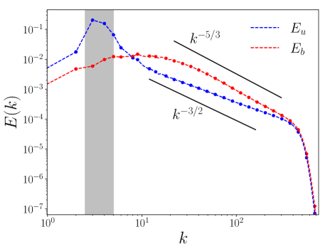
Figure 1: Time-averaged omnidirectional spectra for the velocity and magnetic field (run A1). The gray region indicates the wavenumber band where the velocity field is forced: $k\in[2.5,5.0]$.

To calculate an effective Reynolds number for a hyperdissipative system we follow the approach described in Buzzicotti et al. (2018). There, the standard (Laplacian dissipation) integral-scale Reynolds number $Re={UL_{u}}/{\nu}\propto(L_{u}/\eta_{1})^{4/3}$ (e.g., Batchelor, 1970; Pope, 2000) is replaced with one based on the ratio between the integral scale $L_{u}$ and the effective dissipation range scale $I_{d}$. Specifically, we employ

$$Re=C\left(\dfrac{L_{u}}{I_{d}}\right)^{4/3},$$ (21)

where $I_{d}=\pi/\text{argmax}\left(k^{2}{E_{u}}(k)\right)$ is the scale where the dissipation spectrum $k^{2}E_{u}(k)$ has a maximum. Here, $C$ is a fit parameter that has to be estimated by comparing eq. (21) with the common definition of the Reynolds number in a standard-viscosity run. Making use of this procedure we obtain $C=40$ and $Re=9931$ for run A1 (table 1). Generalization of the Reynolds number for systems with hyper-dissipation has been discussed in Spyksma et al. (2012).

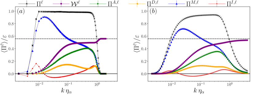
Figure 2: Terms contributing to the MHD filtered energy flux across scale $\ell$, along with the resolved-scale-conversion (kinetic to magnetic) term, as function of the adimensional parameter $k\eta_{\alpha}=\pi\eta_{\alpha}/\ell$: (a) Fourier filter, (b) Gaussian filter. All terms are normalized by the mean total energy dissipation rate $\varepsilon=\varepsilon_{u}+\varepsilon_{b}$. The dashed horizontal line indicates the normalized magnetic dissipation rate $\varepsilon_{b}/\varepsilon$. The errorbars, although not fully visible, indicate one standard error. See eqns (6)–(7).

Figure 2 displays the four MHD energy subfluxes, introduced in eqs. (6)–(7), and their sum. Also shown is ${\cal W}^{\ell}$, the resolved-scale-conversion of kinetic energy to magnetic energy (recall this does not represent energy transfer across $\ell$). The two panels present fluxes obtained through different filters, results shown in fig. 2(a) correspond to Galerkin truncation, and those shown in fig. 2(a) to the Gaussian filter of eq. (12). The data shown in fig. 2(a) and (b) are qualitatively similar but with quantitative differences. Focusing on the similarities, we see that the Inertial term $\langle\Pi^{I,\ell}\rangle$ is relatively weak and is the only one to exhibit inverse transfer regions, in the intervals $1.5\times 10^{-2}\lesssim k\eta_{\alpha}\lesssim 2\times 10^{-1}$ and $4\times 10^{-3}\lesssim k\eta_{\alpha}\lesssim 6\times 10^{-3}$. All the other subfluxes are associated with a direct cascade from the large to the small scales. The energy transfer from the momentum equation of eq. (6) is almost entirely dominated by the Maxwell subflux ($-\Pi^{M,\ell}$) whose peak occurs in proximity to the forcing region. In contrast, the advection term from the induction equation ($\Pi^{A,\ell}$) is peaked at the small scales, close to the dissipative range. The conversion term, ${\cal W}^{\ell}$, is positive and increases monotonically with $k\eta_{\alpha}$. Particularly for the Fourier filter, it is roughly constant (i.e., scale independent) in the region $0.2\lesssim k\eta_{\alpha}\lesssim 0.9$ where kinetic and magnetic subfluxes are in equipartition (Bian & Aluie, 2019); see fig. 10 in Appendix D. Also evident is a sudden increase of ${\cal W}^{\ell}$ in the dissipative range ($k\eta_{\alpha}\gtrsim 1$), due to hyperdiffusion, where the conversion rate saturates to $\varepsilon_{b}$ as already pointed by Bian & Aluie (2019).

Turning to the differences between the two kinds of filtering, we observe that the bandwidth of the inertial range plateau is narrower for the Gaussian filter case, roughly $k\eta_{\alpha}\in[0.04,0.4]$ versus $k\eta_{\alpha}\in[0.013,0.7]$. In general for the Gaussian filtering peaks are of lower amplitude and a little less localised. Linked to this is a more gradual roll-off of the fluxes at high $k\eta_{\alpha}$ and a slower convergence of ${\cal W}^{\ell}$ to $\varepsilon_{b}$ with increasing $k$. These effects arise because Gaussian filtering at scale $\ell$ retains some effects from scales $\leq\ell$, unlike the situation for the sharp Galerkin truncation of the Fourier filter. For $\Pi^{D,\ell}$ there is also a qualitative difference, with the high-$k$ local minimum and maximum seen with the Fourier filter essentially absent when the Gaussian filter is used.

4 Analysis and Discussion

4.1 Inertial flux and comparison with hydrodynamics

The exact decomposition of the Inertial term $\Pi^{I,\ell}$, eq. (8), is

$$\Pi^{I,\ell}=\Pi^{I,\ell}_{s,SSS}+\Pi^{I,\ell}_{m,SSS}+\Pi^{I,\ell}_{s,S\Omega\Omega}+\Pi^{I,\ell}_{m,S\Omega\Omega}+\Pi^{I,\ell}_{m,S\Omega S},$$ (22)

where $\Pi^{I,\ell}_{s,S\Omega S}$ is not included as it is identically zero. This is the special case of eq. (35) where all the fields are the velocity and naturally it coincides with the original decomposition provided by Johnson (2020) for Navier–Stokes turbulence. It is thus of interest to investigate whether there are differences between the HD and MHD instances of eq. (22), and how these might arise.

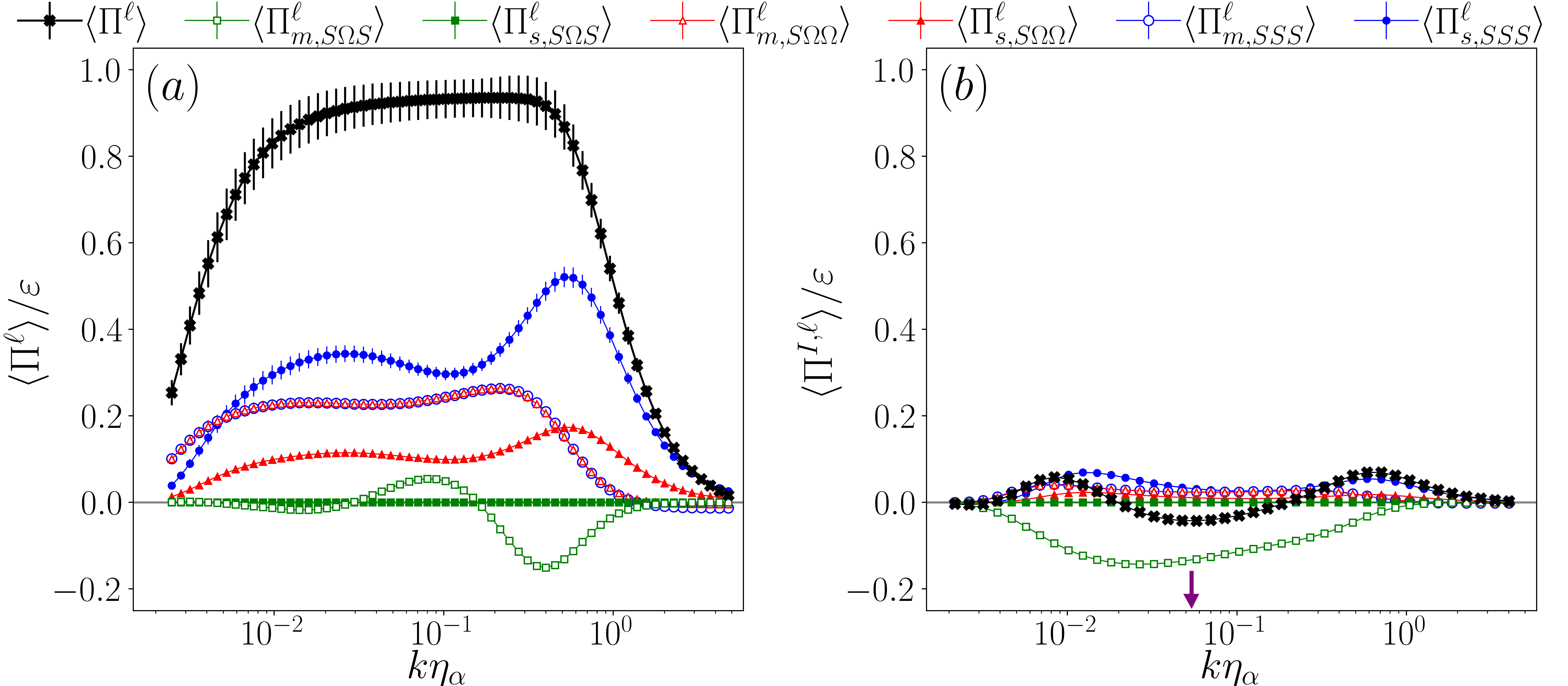
Figure 3: Contributions to the Inertial energy flux $\langle\Pi^{I,\ell}\rangle$ for (a) the HD dataset H2 and (b) the MHD dataset A1, as a function of the (nondimensionalized) reciprocal scale $\ell$, i.e., $k\eta_{\alpha}=\pi\eta_{\alpha}/\ell$. All fluxes are normalised by the mean total energy dissipation rate $\varepsilon$ for the dataset. Filled symbols correspond to single-scale contributions while hollow markers indicate multi-scale contributions. Errorbars are for one standard error. Both panels indicate that $\langle\Pi^{I,\ell}_{m,SSS}\rangle\approx\langle\Pi^{I,\ell}_{m,S\Omega\Omega}\rangle$. In (b) the purple arrow locates $k\eta_{\alpha}=5.4\times 10^{-2}$ (equivalent to $kL_{u}\approx 14$), the value used for the p.d.f.s shown in figures 4, 7, and 9.

Figure 3 compares these two cases. For the hydrodynamic case, panel (a), there is a relatively clear and extended plateau for the total flux (and some of the subfluxes) corresponding to an inertial range. In contrast, the MHD case shown in panel (b) lacks such a plateau and the individual subfluxes are mostly much smaller than their hydrodynamic counterparts. Indeed, only $\langle\Pi^{I,\ell}_{m,SS\Omega}\rangle$ has values comparable to its hydrodynamic counterpart, albeit with a different functional form, being negative for almost all $k$. Intriguingly, this term is the only one that does not vanish point-wise in 2D turbulence, as Johnson (2021) has discussed. A depletion of the inertial flux in MHD turbulence has been observed by Alexakis (2013) and Yang et al. (2021) for configurations with large-scale electromagnetic forcing and by Offermans et al. (2018) for a saturated dynamo at lower Reynolds number. We have verified that the Betchov (1956) relation, $\langle{\Pi^{I,\ell}_{s,SSS}}\rangle=3\langle{\Pi^{I,\ell}_{s,S\Omega\Omega}}\rangle$, holds for both datasets, as it must.

Also of interest is that there appears to be an approximate multi-scale analog of the Betchov relation, with $\langle\Pi^{I,\ell}_{m,SSS}\rangle\approx\langle\Pi^{I,\ell}_{m,S\Omega\Omega}\rangle$. For hydrodynamics, this was already noted in Johnson (2021) and justified by Yang et al. (2023). Evidently this approximate degeneracy also holds in this MHD situation, although the smallness of the terms makes this difficult to appreciate from Figure 3(b).

Having discussed mean fluxes, we now examine some statistical properties of their pointwise contributions. Figure 4 presents standardised probability density functions (p.d.f.s) of the MHD Inertial subfluxes at $k\eta_{\alpha}=5.4\times 10^{-2}$. It is evident that the distributions are strongly non-Gaussian and exhibit very wide tails, with fluctuations at tens of standard deviations. (As we shall see, this is a common characteristic for all the MHD energy fluxes and subfluxes.) The variance, skewness, and kurtosis for each p.d.f. are reported in table 2. Although the p.d.f. of $\Pi_{s,S\Omega\Omega}^{I,\ell}$, that corresponds to the scale-local vortex stretching, has more asymmetrical tails than those of $\Pi_{s,SSS}^{I,\ell}$, the skewness for the latter is nonetheless larger. The term $\Pi_{s,S\Omega S}^{I,\ell}$ does not show up in fig. 4 because it is identically zero due to the symmetries of the tensors involved in the corresponding trace of eq. (35). On the contrary the right panel shows that $\Pi_{m,S\Omega S}^{I,\ell}$ is the most negatively skewed p.d.f. among the Inertial ones.

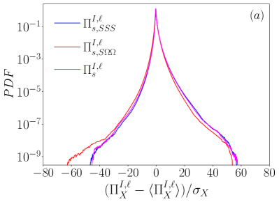
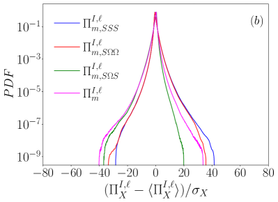
Figure 4: Standardised p.d.f.s of the MHD Inertial subfluxes $\Pi^{I,\ell}_{X}$ at $k\eta_{\alpha}=5.4\times 10^{-2}$ (equivalent to $kL_{u}=14$) from dataset A1, where $X$ identifies the specific subflux. (a) single-scale fluxes; (b) multi-scale fluxes.

In connection with the approximate degeneracy between $\langle\Pi^{I,\ell}_{m,SSS}\rangle$ and $\langle\Pi^{I,\ell}_{m,S\Omega\Omega}\rangle$ discussed above, fig. 4(b) reveals that their p.d.f.s coincide up to events with a standardised probability density of $\sim 10^{-7}$, potentially indicating that the approximate identity is true not just on average but also for higher-order moments, although further analysis is required.

4.2 Maxwell flux

The decomposition of the energy flux associated with the Lorentz force, which we refer to as the Maxwell term, $\Pi^{M,\ell}$ of eq. (9), contains an extra (single-scale) term with respect to the Inertial flux. Specifically, from eq. (35) we obtain

$$\Pi^{M,\ell}=\Pi^{M,\ell}_{s,S\Sigma\Sigma}+\Pi^{M,\ell}_{m,S\Sigma\Sigma}+\Pi^{M,\ell}_{s,SJJ}+\Pi^{M,\ell}_{m,SJJ}+\Pi^{M,\ell}_{s,SJ\Sigma}+\Pi^{M,\ell}_{m,SJ\Sigma}.$$ (23)

Terms of type $S\Sigma\Sigma$ can be associated with strain rate amplification by magnetic shear, while terms of type $SJJ$ correspond to current-filament stretching that is analogous to vortex stretching in HD. The last two terms are of type $SJ\Sigma$ and describe the back-reaction of the magnetic field on the flow, or more specifically how the velocity strain rate is modified (typically amplified) in connection with a current-sheet thinning process. As we shall see, this is by far the dominant process. It proceeds as follows (fig. 5). First, a current sheet is stretched by large-scale straining motions into a magnetic shear layer, in a process similar to vortex thinning in HD (Kraichnan, 1976; Chen et al., 2006; Johnson, 2021). This results in a stretching of the magnetic flux tubes in the sheet. By conservation of magnetic flux, the magnetic field strength at the thereby generated smaller scales must increase. That is, magnetic energy is transferred from large to small scales. (We will revisit this process in section 4.3 in the context of the inter-scale transfer of magnetic energy.) The magnetic rate-of-strain field associated with the resulting magnetic shear layer now accelerates fluid along its extensional directions and slows it down in the compressional directions, thereby generating a stronger rate-of-strain field across smaller scales.

It is instructive to consider the process in two dimensions, in analogy to the vortex thinning of 2D HD (Johnson, 2021). In the reference frame of the rate-of-strain tensor at scale $\ell$, the associated terms are

$$\Pi^{M,\ell}_{s,SJ\Sigma}(\bm{x}) =2\lambda_{S}^{\ell}(\bm{x})\lambda^{\ell}_{\Sigma}(\bm{x})\overline{j}^{\ell}(\bm{x})\sin{2\psi(\bm{x})}\ ,$$ (24)

$$\Pi^{M,\ell}_{m,SJ\Sigma}(\bm{x}) =2\int_{0}^{\ell^{2}}\mathrm{d}\theta\int_{\mathbb{R}^{3}}G^{\phi}(\bm{r})\lambda_{S}^{\ell}(\bm{x})\lambda^{\sqrt{\theta}}_{\Sigma}(\bm{x}+\bm{r})\overline{j}^{\sqrt{\theta}}(\bm{x}+\bm{r})\sin{2\psi(\bm{x}+\bm{r})}\ ,$$ (25)

where $\pm\lambda_{S}$ and $\pm\lambda_{\Sigma}$ are the eigenvalues of the velocity and magnetic rate-of-strain tensors, respectively, $\psi$ the angle between the respective eigenvectors, and $j$ the out-of-plane component of the current density. As can be seen from these formulae, a maximum energy transfer occurs when the principal axes of the magnetic rate-of strain tensor have a $\pm 45^{\circ}$ angle to those of the velocity rate-of-strain tensor. Depending on the sign of the out-of-plane current density and $\sin(2\psi)$, eqs. (24) and (25) result in a direct or an inverse cascade. Figure 5 presents a schematic depiction of the process. A direct cascade occurs if the angle between the principal axes of velocity and magnetic strain-rate tensors is in the same rotational direction as the out-of-plane current. A similar, albeit less straightforward, assessment is possible in three dimensions, where

$$\Pi^{M,\ell}_{s,SJ\Sigma}(\bm{x})=2\ell^{2}\overline{S}_{ij}^{\ell}\overline{J}^{\ell}_{ik}\overline{\Sigma}^{\ell}_{kj}=2\ell^{2}\sum_{i=1}^{3}\sum_{j=1}^{3}\lambda^{\ell}_{i}\mu_{j}^{\ell}\cos^{2}{\psi_{ij}},$$ (26)

and similarly for the multi-scale term. Here, $\mu^{\ell}_{j}$ is the $j$-th eigenvalue of the symmetric part of the product matrix $\overline{J}^{\ell}_{ik}\overline{\Sigma}^{\ell}_{kj}$ (a contribution to the Maxwell SGS stress tensor) and $\psi_{ij}$ the angle between the $i$-th eigenvector of $\overline{\bm{S}}^{\ell}$ and the $j$-th eigenvector of the symmetric part of $\overline{J}^{\ell}_{ik}\overline{\Sigma}^{\ell}_{kj}$. For a forward cascade of kinetic energy, $\langle\Pi^{M,\ell}\rangle>0$, which implies that $\overline{S}^{\ell}_{ij}\overline{J}^{\ell}_{ik}\overline{\Sigma}^{\ell}_{kj}$ should be preferentially positive. Due to the presence of the cosine squared factor, this implies that the principal axes of the rate-of-strain tensor and those of the subscale stress must preferentially align, resulting in a stretching of the magnetic flux tubes along the extensional directions of the strain-rate tensor, as discussed above.

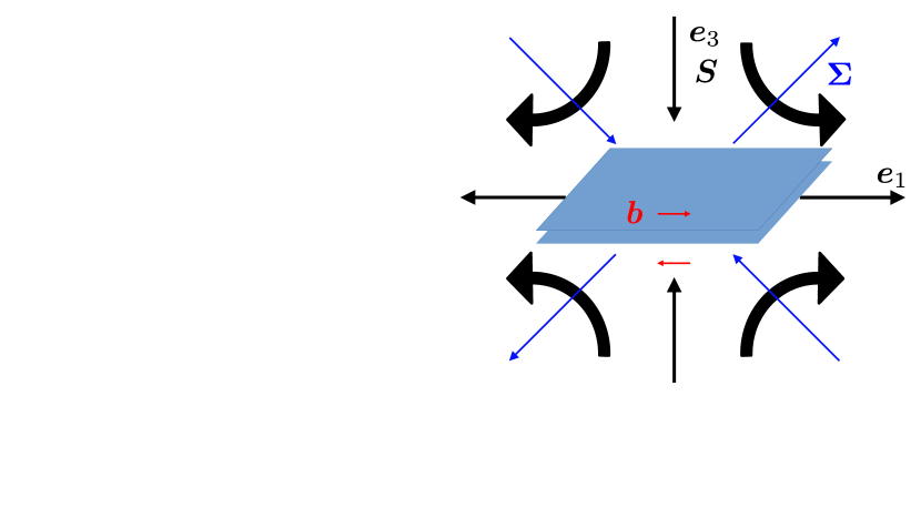
Figure 5: Two-dimensional sketch of current-sheet thinning and strain rate amplification by the latter. A current sheet, $\bm{J}$, is stretched by large-scale strain, $\bm{S}$ (left) into a magnetic shear layer (right, red arrows). This induces a stretching of the magnetic flux tubes in the sheet. By conservation of magnetic flux, the magnetic field strength at the thereby generated smaller scales increases. That is, magnetic energy is transferred from large to small scales. The resulting magnetic shear layer has an associated magnetic strain rate field, $\bm{\Sigma}$, whose principal axes (solid blue arrows) are at $45^{\circ}$ to those of the large-scale strain rate tensor (straight black arrows). As the magnetic shear will align with the extensional direction of the (velocity) strain rate tensor, this causes the fluid to be accelerated along these extensional directions and slowed down in the compressional directions, thereby generating a stronger rate-of-strain field across smaller scales, $\bm{S}^{\prime}$, indicated by the dashed arrows. The principal axes of the large-scale strain rate tensor are denoted by $\bm{e}_{1}$ in one extensional direction and $\bm{e}_{3}$ in one compressional direction and analogously for the small-scale strain rate.

The subfluxes on the RHS of eq. (23) and the total Maxwell flux are shown in fig. 6, as a function of (nondimensionalised) reciprocal $\ell$. We see immediately that the net energy transfer proceeds from large scales to small scales with the total Maxwell flux $\langle\Pi^{M,\ell}\rangle$ being the dominant energy subflux for MHD, carrying approximately $80\%$ of the total energy dissipation rate at its peak. At large scales, the major contribution is from the multi-scale term $\langle\Pi^{M,\ell}_{m,SJ\Sigma}\rangle$, switching to its single-scale partner, $\langle\Pi^{M,\ell}_{s,SJ\Sigma}\rangle$, as the dissipation scale is approached. All remaining terms in eq. (23), are negligible. Summarising the mean Maxwell flux behaviour, we may say that the net kinetic energy transfer in MHD proceeds by the back-reaction of the magnetic field on the flow during the aforementioned current-sheet thinning process, while the contribution from current filament stretching and strain-amplification by magnetic shear are negligible.

The p.d.f.s for the Maxwell energy fluxes are shown in fig. 7. The predominance of $\langle\Pi^{M,\ell}_{m,SJ\Sigma}\rangle$ in the direct cascade can be also appreciated by examining its p.d.f., which is the most positively-skewed among the multi-scale terms of fig. 7; see also table 2 for p.d.f. moments. As can be seen from the data shown in fig. 7, while all terms of type $S\Sigma\Sigma$ and $SJJ$ nearly vanish on average, fluctuations around 60 standard deviations are not uncommon, and their multi-scale contributions show considerable backscatter.

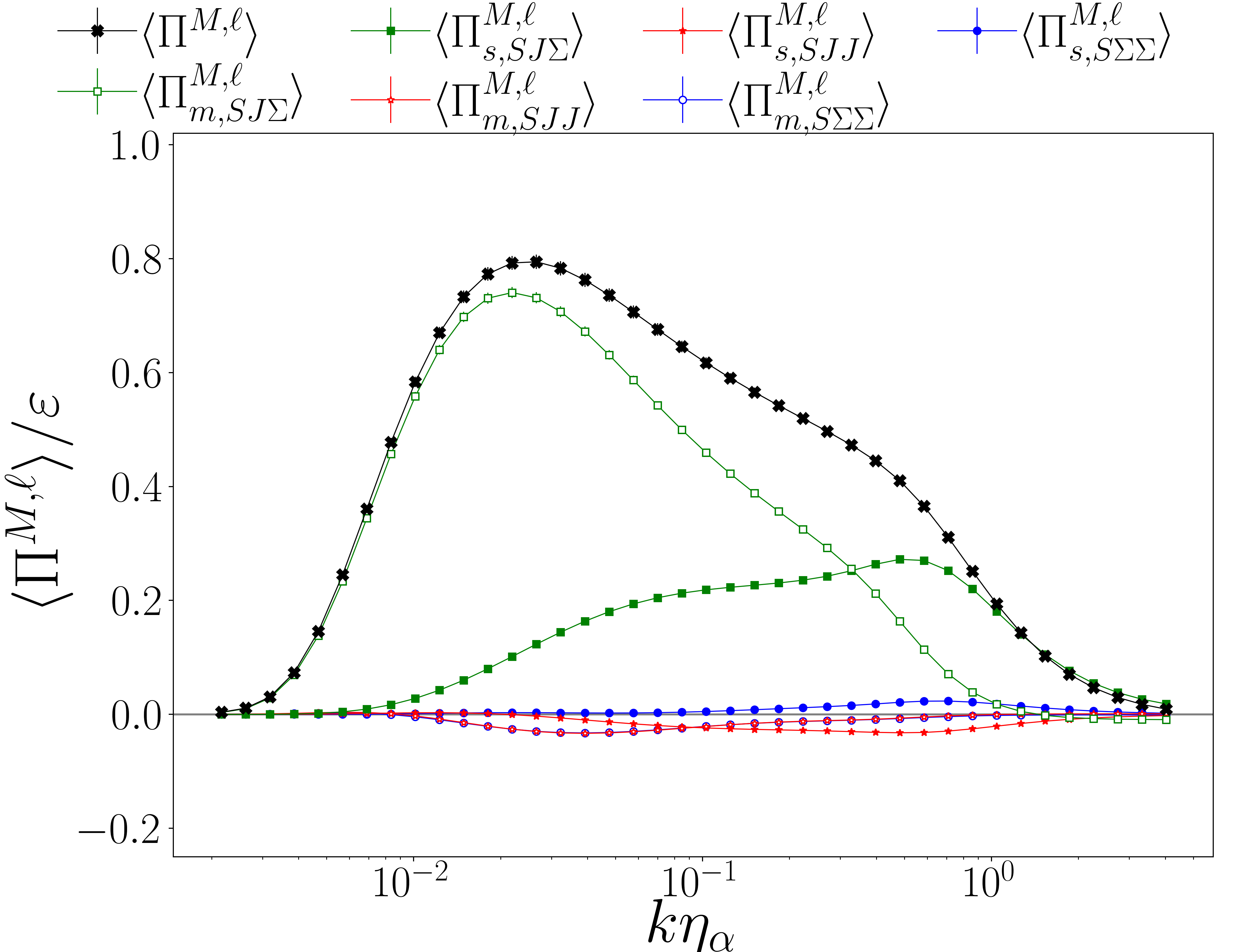
Figure 6: Contributions to the Maxwell energy flux $\langle\Pi^{M,\ell}\rangle$. Data is from dataset A1 and normalised by the mean total energy dissipation rate $\varepsilon$. Errorbars indicate one standard error.

In Appendix B we show that the averages of the subfluxes $\Pi^{M,\ell}_{m,S\Sigma\Sigma}$ and $\Pi^{M,\ell}_{m,SJJ}$ can be connected via an exact Betchov-like relation that holds for all homogeneous flows

$$\langle\Pi^{M,\ell}_{m,S\Sigma\Sigma}\rangle=\langle\Pi^{M,\ell}_{m,SJJ}\rangle+2\langle\Pi_{m,\Omega\Sigma J}^{M,\ell}\rangle.$$ (27)

Note that the final term, $\langle\Pi_{m,\Omega\Sigma J}^{M,\ell}\rangle$, does not appear in the Maxwell flux, eq. (23), and our numerical results indicate $\langle\Pi^{M,\ell}_{m,S\Sigma\Sigma}\rangle\approx\langle\Pi^{M,\ell}_{m,SJJ}\rangle$, see fig. 6. Physically, we may interpret this approximate identity as indicating that the net “strain-production” by magnetic shear is almost equal to the net strain production by current-filament stretching. However we stress again that these contributions to the interscale kinetic energy transfer are negligible. Further discussion on terms associated with strain production and current-filament stretching is provided in Appendix  B.

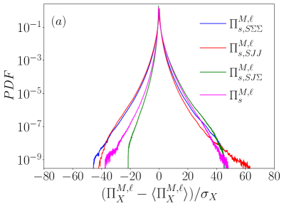
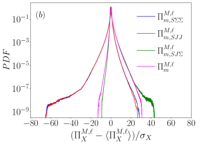
Figure 7: Standardised p.d.f.s for Maxwell subfluxes $\Pi^{M,\ell}_{X}$, at $k\eta_{\alpha}=5.4\times 10^{-2}$, from dataset A1, where $X$ represents the subflux identifier. (a) single-scale fluxes; (b) multi-scale fluxes. Note that the p.d.f.s for $\Pi^{M,\ell}_{m,S\Sigma\Sigma}$ and $\Pi^{M,\ell}_{m,SJJ}$ are approximately coincident.

4.3 Advection and Dynamo fluxes

In this section we focus on the decomposition of both the Advection term, $\Pi^{A,\ell}$, and the Dynamo term, $\Pi^{D,\ell}$, as defined in eqs. (10)–(11). As is well known these two SGS fluxes share the same physical origin, namely the induced (fluctuation) electric field, and this is associated with certain symmetries and equivalences between the Advection and Dynamo subfluxes.

From the application of eq. (35), we find:

$$\Pi^{A,\ell}=\ \Pi^{A,\ell}_{s,\Sigma\Sigma S}+\Pi^{A,\ell}_{m,\Sigma\Sigma S}+\Pi^{A,\ell}_{m,\Sigma\Sigma\Omega}+\Pi^{A,\ell}_{s,\Sigma JS}+\Pi^{A,\ell}_{m,\Sigma JS}+\Pi^{A,\ell}_{s,\Sigma J\Omega}$$ (28)

$$+ \Pi^{A,\ell}_{m,\Sigma J\Omega}+\Pi^{A,\ell}_{s,J\Sigma S}+\Pi^{A,\ell}_{m,J\Sigma S}+\Pi^{A,\ell}_{s,J\Sigma\Omega}+\Pi^{A,\ell}_{m,J\Sigma\Omega}+\Pi^{A,\ell}_{s,JJS}+\Pi^{A,\ell}_{m,JJS}+\Pi^{A,\ell}_{m,JJ\Omega},$$

$$\Pi^{D,\ell}=\ \Pi^{D,\ell}_{s,\Sigma S\Sigma}+\Pi^{D,\ell}_{m,\Sigma S\Sigma}+\Pi^{D,\ell}_{s,\Sigma SJ}+\Pi^{D,\ell}_{m,\Sigma SJ}+\Pi^{D,\ell}_{m,\Sigma\Omega\Sigma}+\Pi^{D,\ell}_{s,\Sigma\Omega J}+\Pi^{D,\ell}_{m,\Sigma\Omega J}$$ (29)

$$+ \Pi^{D,\ell}_{s,JS\Sigma}+\Pi^{D,\ell}_{m,JS\Sigma}+\Pi^{D,\ell}_{s,JSJ}+\Pi^{D,\ell}_{m,JSJ}+\Pi^{D,\ell}_{s,J\Omega\Sigma}+\Pi^{D,\ell}_{m,J\Omega\Sigma}+\Pi^{D,\ell}_{m,J\Omega J},$$

where we do not list terms that vanish identically, see Appendices A and E.

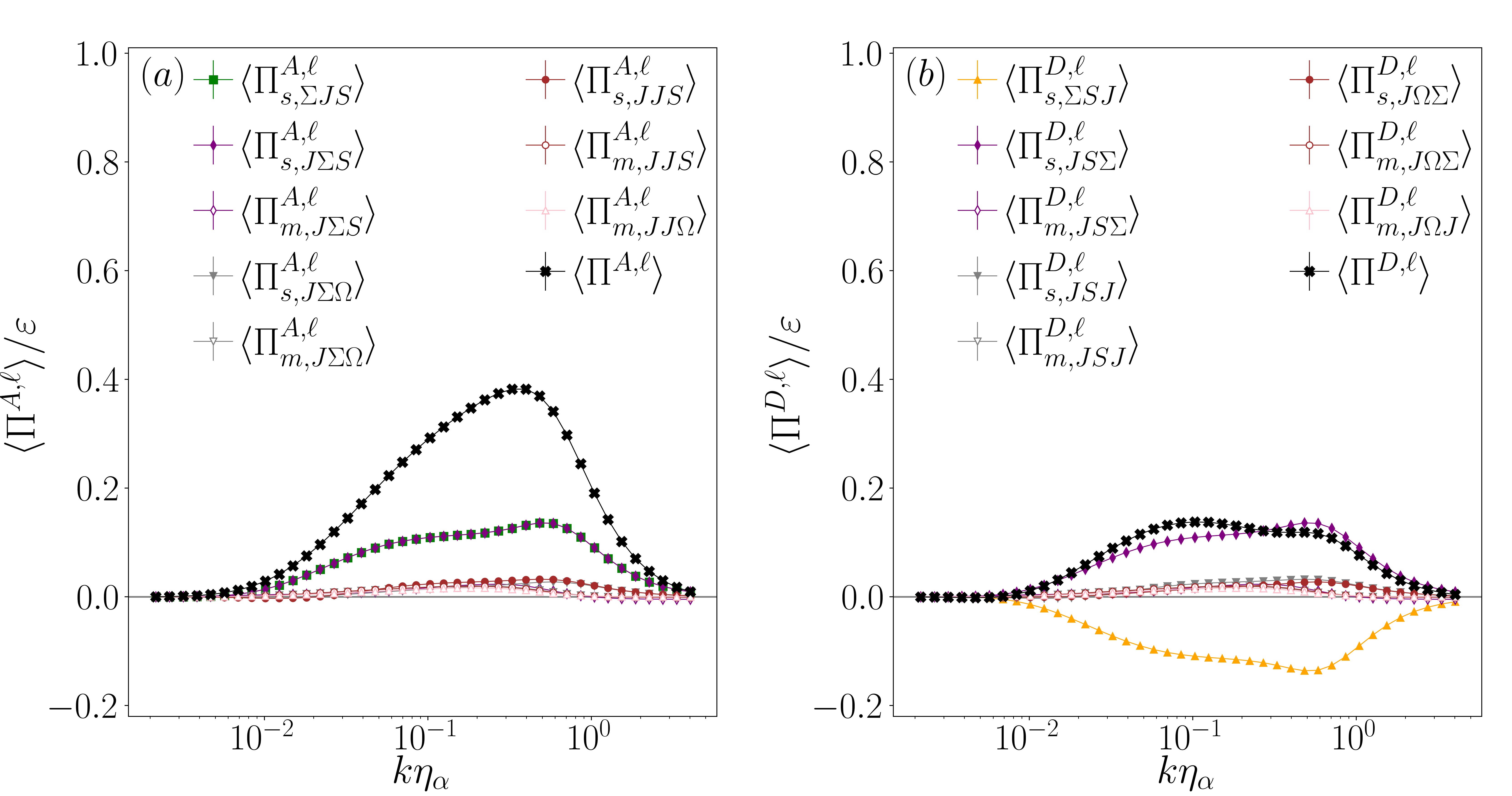
Figure 8: Decomposed fluxes for the (a) Advection term $\langle\Pi^{A,\ell}\rangle$ and (b) Dynamo term $\langle\Pi^{D,\ell}\rangle$. Fluxes are normalised by the mean total energy dissipation rate $\varepsilon$ for dataset A1. In panel (a) $\langle\Pi^{A,\ell}_{s,\Sigma JS}\rangle$ and $\langle\Pi^{A,\ell}_{s,J\Sigma S}\rangle$ perfectly coincide. The errorbars indicate one standard error.

Figure 8 displays most of the Advection and Dynamo (sub)fluxes in separate panels. For clarity, only the subfluxes relevant to the discussion below and to the net energy flux are shown. The cyclic property of the trace can be used to show that some terms vanish identically and that each Advection subflux (both single-scale and multi-scale) is equal to (plus or minus) a partner Dynamo subflux; see the subfluxes expressions in Appendix E. For this reason in fig. 8 the following subflux pairs are not displayed since they are opposite in sign, $\langle\Pi^{A,\ell}_{s,\Sigma\Sigma S}\rangle$ and $\langle\Pi^{D,\ell}_{s,\Sigma S\Sigma}\rangle$ as well as $\langle\Pi^{A,\ell}_{s,\Sigma J\Omega}\rangle$ and $\langle\Pi^{D,\ell}_{s,\Sigma\Omega J}\rangle$ together with their multi-scale counterparts. Hence, these cancel pairwise and make no contribution to the net magnetic energy flux $\Pi^{A,\ell}+\Pi^{D,\ell}$; see Appendix E. In contrast, $\langle\Pi^{A,\ell}_{s,JJS}\rangle$ and $\langle\Pi^{D,\ell}_{s,JSJ}\rangle,$ and the related multi-scale terms, are equal and thus do contribute to the net flux. Note, too, that the two Betchov relations eqs. (51)–(55) can provide another source of symmetry, or approximate symmetry.

The physical interpretation of the respective terms is very similar to what has been discussed for the Maxwell flux, except that now the effect of the flow on the magnetic field must be considered. Recall from sec 4.2 that the Maxwell flux terms of type $SJ\Sigma$ correspond to the stretching and, by incompressibility, thinning of current sheets into magnetic shear layers. And that the back-reaction on the flow induced by this process is responsible for the bulk of the kinetic energy transfer to smaller scales. As we shall see, and as expected from the discussion of current-sheet thinning in section 4.2, this process also transfers most magnetic energy from large to small scales. However, in contrast to the Maxwell flux situation (dominated by a multiscale term), here it is two of the Advection single-scale terms, $\Sigma JS$ and $J\Sigma S$, that carry most of the magnetic energy flux.

Focusing on the Advection term, from fig. 8(a) we observe that the net flux is everywhere positive and peaked at smaller scales, roughly at the end of the inertial range. Recall that the Maxwell flux is peaked at larger scales (fig. 6). Due to the cyclic property of the trace the terms $\Pi^{A,\ell}_{s,\Sigma JS}$ and $\Pi^{A,\ell}_{s,J\Sigma S}$ are equal while, because of the symmetry of the tensors involved, the subfluxes $\Pi^{A,\ell}_{s,JJ\Omega}$ and $\Pi^{A,\ell}_{s,\Sigma\Sigma\Omega}$ together with $\Pi^{D,\ell}_{s,J\Omega J}$ and $\Pi^{D,\ell}_{s,\Sigma\Omega\Sigma}$ are identically zero. It is also apparent from fig 8(a) that the remaining Advection terms make negligible contributions to the net flux. We note that $\Sigma\Sigma S$ type terms correspond to magnetic shear amplification due to straining motions and those of type $JJS$ to current filament stretching. Terms of type $\Sigma J\Omega$ encode a correlation between current and vorticity. Thus, the net Advection term is primarily due to single-scale contributions, being approximately equal to $2\Pi^{A,\ell}_{s,\Sigma JS}$, and it carries about $40\%$ of the total energy flux at its peak.

For the Dynamo term, $\Pi^{D,\ell}$, we observe that the net flux is almost flat in the inertial range, substantially positive definite for these scales (fig. 8(b)) and responsible for about $15\%$ of the total energy flux. All subfluxes except $\Pi^{D,\ell}_{s,\Sigma SJ}$ shown in yellow and $\Pi^{D,\ell}_{s,JS\Sigma}$ indicated by the filled purple symbols are negligible. However, using the cyclic property once again, one can show that $\Pi^{D,\ell}_{s,\Sigma SJ}=-\Pi^{D,\ell}_{s,JS\Sigma}$ hence these two terms cancel out and do not contribute to the net flux. In contrast to the Advection term, the major contributions to the net Dynamo term are from subleading single and multiscale subfluxes of various types, with each contributing only 1–2% to the total energy flux adding up to a total of around $15\%$ of the total energy flux. In summary, single-scale current-sheet thinning is the dominant process transferring magnetic energy across scales. It solely originates from the advective term in the induction equation.

Consider now the p.d.f.s. As a consequence of the symmetries between Dynamo and Advection subfluxes, only the Advection p.d.f.s are shown in panels (a) and (c) of figure 9, respectively for the single-scale terms and the multi-scale terms. It is striking that the p.d.f. of $\Pi^{A,\ell}_{s,\Sigma J\Omega}$ is by far the most strongly fluctuating with huge fluctuations of more than 100 standard deviations. The other Advection subflux p.d.f.s, both single-scale and multi-scale, span a range comparable with those associated with the p.d.f.s for the Inertial and Maxwell fluxes. Moreover, all the multi-scale fluxes (Advection and Dynamo) have quite similar p.d.f.s, and thus so do the net multi-scale flux p.d.f.s (fig. 9(d)). In the case of the net single-scale p.d.f.s, the Advection–Dynamo agreement is still good in the cores of the distributions, but there is a significant difference at larger negative fluctuations (fig. 9(b)).

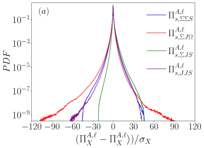
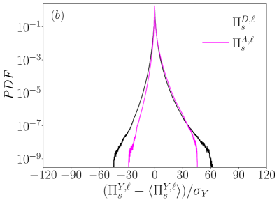
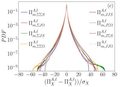
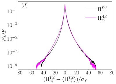
Figure 9: Standardised p.d.f.s for dataset A1 at $k\eta_{\alpha}=5.4\times 10^{-2}$. (a) single-scale Advection subfluxes $\Pi^{A,\ell}_{X}$, where $X$ represents the subflux identifier, and (b) net single-scale fluxes for the Dynamo ($\Pi^{D,\ell}_{s}$) and Advection terms ($\Pi^{A,\ell}_{s}$). In the $x$-axis titles for panels (b) and (d), $Y=A$ or $D$, as appropriate. Note that $\Pi^{A,\ell}_{s,\Sigma JS}=\Pi^{A,\ell}_{s,JS\Sigma}$ (see fig. 8). (c)–(d): as for panels (a)–(b) except for the multi-scale subfluxes of $\Pi^{A,\ell}$ and $\Pi^{D,\ell}$. Note that panels (c)-(d) have the same x-axis range as figures 4–7.

4.4 Total energy flux, $\Pi^{\ell}$

In the preceding subsections we analysed the four contributions to the incompressible MHD energy flux, finding that each of them may be reasonably well approximated using just some of the subfluxes. These approximation may now be assembled to give an approximate form for the mean total MHD energy flux. Specifically we suggest that

$$\langle\Pi^{\ell}\rangle =\langle\Pi^{I,\ell}\rangle+\langle\Pi^{M,\ell}\rangle+\langle\Pi^{A,\ell}\rangle+\langle\Pi^{D,\ell}\rangle\approx-2\langle\Pi^{M,\ell}_{s,SJ\Sigma}\rangle-\langle\Pi^{M,\ell}_{m,SJ\Sigma}\rangle$$ (30)

$$=4\ell^{2}\left\langle\mathrm{Tr}\left\{{(\overline{\bm{S}}^{\ell})^{t}\overline{\bm{J}}^{\ell}(\overline{\bm{\Sigma}}^{\ell})^{t}}\right\}\right\rangle$$ (31)

$$+2\left\langle\int_{0}^{\ell^{2}}\mathrm{d}\theta\,\mathrm{Tr}\left\{{\big{(}\overline{\bm{S}}^{\ell}\big{)}^{t}\Big{(}\overline{\overline{\bm{J}}^{\sqrt{\theta}}\big{(}\overline{\bm{\Sigma}}^{\sqrt{\theta}}\big{)}^{t}\,}^{\phi}-\overline{\overline{\bm{J}}^{\sqrt{\theta}}\,}^{\phi}\;\overline{\big{(}\overline{\bm{\Sigma}}^{\sqrt{\theta}}\big{)}^{\!t}\,}^{\phi}\Big{)}}\right\}\right\rangle$$ (32)

is a suitable expression. Note that, after using cyclic properties of the trace, this is expressed only in terms of two of the Maxwell subfluxes, one single-scale and one multi-scale. These are discussed in sec. 4.2 and we remind the reader that all subflux definitions can be found in Appendix E. Interestingly, the terms on the RHS of eq. (32) are part of a group of terms that remain non-zero in 2D MHD; see Appendix C. We intend to explore this intriguing feature in future work.

Equation (32) demonstrates that the mean total energy flux in MHD turbulence is largely given by the stretching and thinning of current-sheets into magnetic shear layers by large-scale strain, resulting in a transfer of magnetic energy from large to small scales. In addition, there is a back-reaction of this process on the flow, whereby the ensuing magnetic strain-rate field accelerates fluid along its extensional directions and slows it down in the compressional directions, thereby generating a stronger strain-rate field across smaller scales, as shown schematically in fig. 5.

4.5 Current-sheet thinning and magnetic reconnection

As a means of inter-scale energy transfer, the current-sheet thinning process can only proceed as described in an inertial range, i.e., at scales where Joule and viscous dissipation are negligible. As the dissipative scales are approached Alfvén’s theorem ceases to hold and magnetic reconnection can occur, with associated changes to the topology of the magnetic field. Interestingly, models of MHD reconnection are geometrically very similar to the inertial-range energy transfer process described here. For example in the Sweet–Parker model a current sheet is thinned by a flow that pushes magnetic field lines closer and closer together. Eventually, when the distance between the field lines approaches scales where Joule dissipation becomes important, the topological conservation of the magnetic field is broken and magnetic field-lines reconnect. That is, the continuation of the current-sheet thinning process described herein, and shown conceptually in fig. 5, to smaller and smaller scales can lead naturally to magnetic reconnection.

	$\Pi^{I,\ell}_{s}$	$\Pi^{I,\ell}_{s,SSS}$	$\Pi^{I,\ell}_{s,S\Omega\Omega}$		$\Pi^{I,\ell}_{m}$	$\Pi^{I,\ell}_{m,SSS}$	$\Pi^{I,\ell}_{m,S\Omega S}$	$\Pi^{I,\ell}_{m,S\Omega\Omega}$
$(\sigma_{X}^{I})^{2}$	1.107	0.652	0.114		2.522	0.107	0.303	0.109
$S^{I}_{X}$	2.958	3.234	1.483		-1.558	1.424	-2.155	1.301
$K^{I}_{X}$	39.18	41.48	29.68		17.15	18.96	15.42	17.50
	$\Pi^{M,\ell}_{s}$	$\Pi^{M,\ell}_{s,S\Sigma\Sigma}$	$\Pi^{M,\ell}_{s,SJJ}$	$\Pi^{M,\ell}_{s,SJ\Sigma}$	$\Pi^{M,\ell}_{m}$	$\Pi^{M,\ell}_{m,S\Sigma\Sigma}$	$\Pi^{M,\ell}_{m,SJ\Sigma}$	$\Pi^{M,\ell}_{m,SJJ}$
$(\sigma_{X}^{M})^{2}$	0.112	0.014	0.0113	0.119	0.353	0.014	0.467	0.014
$S^{M}_{X}$	3.207	0.326	-0.827	4.030	3.105	-2.176	3.417	-2.289
$K^{M}_{X}$	32.22	32.71	31.09	39.88	21.34	27.96	24.60	28.46
	$\Pi^{A,\ell}_{s}$	$\Pi^{A,\ell}_{s,\Sigma\Sigma S}$	$\Pi^{A,\ell}_{s,\Sigma J\Omega}$	$\Pi^{A,\ell}_{s,\Sigma JS}$	$\Pi^{A,\ell}_{s,J\Sigma S}$	$\Pi^{A,\ell}_{s,JJS}$
$(\sigma_{X}^{A})^{2}$	0.206	0.014	0.004	0.030	0.030	0.011
$S^{A}_{X}$	3.801	-0.333	-2.349	3.843	3.843	0.82
$K^{A}_{X}$	42.16	32.71	53.12	38.90	39.90	31.08
	$\Pi^{A,\ell}_{m}$	$\Pi^{A,\ell}_{m,\Sigma S\Sigma}$	$\Pi^{A,\ell}_{m,\Sigma\Sigma\Omega}$	$\Pi^{A,\ell}_{m,\Sigma J\Omega}$	$\Pi^{A,\ell}_{m,\Sigma JS}$	$\Pi^{A,\ell}_{m,J\Sigma S}$	$\Pi^{A,\ell}_{m,JJS}$	$\Pi^{A,\ell}_{m,J\Sigma\Omega}$	$\Pi^{A,\ell}_{m,JJ\Omega}$
$(\sigma_{X}^{A})^{2}$	0.084	0.003	0.006	0.002	0.007	0.003	0.002	0.002	0.001
$S^{A}_{X}$	0.334	-1.616	-0.743	-2.011	-0.283	0.534	1.34	1.13	1.02
$K^{A}_{X}$	28.99	24.04	25.74	25.92	24.45	26.22	27.48	27.20	29.75
	$\Pi^{D,\ell}_{s}$	$\Pi^{D,\ell}_{m}$
$(\sigma_{X}^{D})^{2}$	0.039	0.055
$S^{D}_{X}$	-1.918	1.804
$K^{A}_{X}$	35.61	25.41

Table 2: Values of variance $(\sigma_{X}^{Y})^{2}$, skewness $S^{Y}_{X}={\left\langle\left(\Pi^{Y,\ell}_{X}-\langle\Pi^{Y,\ell}_{X}\rangle\right)^{3}\right\rangle}/{(\sigma_{X}^{Y})^{3}}$, and kurtosis $K^{Y}_{X}={\left\langle\left(\Pi^{Y,\ell}_{X}-\langle\Pi^{Y,\ell}_{X}\rangle\right)^{4}\right\rangle}/{(\sigma_{X}^{Y})^{4}}$ for the subflux p.d.f.s shown in figs.04–9, where $X$ indicates the subflux identifier and $Y$ denotes the term identifier.

5 Consequences for MHD subgrid-scale modelling

MHD LES modelling usually proceeds through variations on the Clark and Smagorinsky models. This is the case for incompressible MHD (Zhou & Vahala, 1991; Müller & Carati, 2002b; Kessar et al., 2016). Moreover, adaptations have been made for the compressible case (Chernyshov et al., 2010; Vlaykov et al., 2016; Grete et al., 2016), for channel flow at high magnetic Reynolds number (Hamba & Tsuchiya, 2010; Jadhav & Chandy, 2021, 2023), and for extensions of MHD taking various levels of microphysics terms into account, such as Hall MHD (Miura et al., 2016) or Braginskii-extended (two-fluid) MHD (Miura et al., 2017), with the latter specifically focussed on the ballooning instability in stellarator devices. Most such approaches use the same SGS model for the inertial and Maxwell stresses based on velocity-field gradients with eddy viscosities involving either only the strain rate tensor or a weighted sum of the squared strain rate and the squared current, and similarly structured SGS models for the induction equation, with either heuristics or trial-and-error approaches to find suitable values for model constants. In what follows, we briefly discuss how the present results can be used to construct suitably structured SGS models for each SGS-stress in the MHD equations.

In terms of SGS modelling, our simulation-based results suggest that the Inertial terms can be neglected and a dissipative model for the Maxwell stresses should suffice to capture the (leading-order) mean effects. In terms of fluctuations, we find that the observed mean Inertial flux depletion is caused by considerable backscatter in all Inertial subfluxes. This could suggest that a more sophisticated model would be required for the Inertial term. However, in 3D HD turbulence, backscatter-free SGS models such as the standard static Smagorinsky closure perform well in capturing high-order statistics, that is anomalous exponents and multifractal predictions for the correlation between velocity-field increments and SGS stresses (Linkmann et al., 2018). Furthermore, as the SGS stresses enter the filtered Navier–Stokes equation only through their divergence, this results in a degree of (gauge) freedom to determine model stress tensors that produce much less backscatter than those constructed using the standard definition (Vela-Martín, 2022). In fact, backscatter can be traced back to spatial fluxes disconnected from the (scale-space) energy transfer and as such does not require modelling (Vela-Martín, 2022).

For the magnetic energy transfers, we observe the net transfers are from large to small scales, suggesting again that dissipative models should suffice. Indeed, as multi-scale terms in our flux decomposition are negligible, a Clark-type model involving only the coupling between current and strain-rate tensors may work well for a nonlinear saturated non-helical (small-scale) dynamo. However, additional stabilising terms may be required as the Clark (or gradient) model is know to result in numerically unstable LES of a mixing layer in HD (Vreman et al., 1996, 1997) and for MHD (Müller & Carati, 2002a; Kessar et al., 2016), as discussed in further detail below. Similar to the Inertial term results, we observe considerable backscatter in the magnetic energy fluxes, and it remains to be seen if the aforementioned results by Linkmann et al. (2018) on the effect of SGS closures on high-order statistics carry over from HD to MHD.

For a nonhelical saturated dynamo, as is the case here, Müller & Carati (2002a) and Kessar et al. (2016) carried out MHD LES with Clark-type models constructed from the full velocity and magnetic-field gradients for the sum of the Reynolds and Maxwell SGS stress in the momentum equation and for the magnetic stresses, resulting in unstable simulations as in the HD case. Using a-priori analyses of DNS data, Kessar et al. (2016) trace the instabilities back to the Clark terms (which correspond to what we have herein called single-scale flux contributions) transferring an insufficient amount of kinetic and magnetic energy to small scales, and to a production of backscatter. According to our analysis, for the momentum equation the former effect is due to the Maxwell stress having a significant multi-scale component which is not captured in the Clark model. Furthermore, a Clark model based on the full gradients will introduce effects that are not present in the full MHD dynamics especially concerning the Maxwell and magnetic stresses, as all combinations of vorticity, strain, current, and magnetic strain are included in the model and equally weighted. Our analysis, however, shows that only terms stemming from the coupling between current and strain-rate tensors are significant, with all remaining contributions to the net Maxwell and magnetic fluxes being negligible. Thus, retaining these contributions in a SGS model may substantially (and inappropriately) affect the small-scale structure of the flow and the magnetic field.

A further challenge for LES modelling of MHD turbulence is to accurately capture the transfer of magnetic to kinetic energy and vice versa. As discussed by Offermans et al. (2018), the resolved-scale conversion term must either be fully accounted for in LES, resulting in the need to resolve all scales where this term is active, or in the present case of a saturated dynamo, a model including an extra term accounting for the under-resolved dynamo effect must be provided.

In this paper we have only considered the no mean magnetic field situation. The presence of a strong background magnetic field is likely to require an SGS modelling approach that differs from those just discussed, as the ensuing anisotropy and two-dimensionalisation of magnetic and velocity-field fluctuations may result in partial inverse fluxes. We will report results on configurations with strong background magnetic fields in due course. Similarly, the large-scale (helical) dynamo requires an investigation in its own right, and the magnetic-field growth at large scales is likely to require a different type of SGS modelling approach, as Kessar et al. (2016) report that the Clark and even a standard static Smagorinsky model result in unstable LES.

The method discussed here can be readily extended to Hall- and two-fluid MHD and other fluid models for plasma turbulence. For instance, the applicability of the Smagorinsky closure to Hall MHD has been assessed by an a-priori analysis using sharp filtering (Miura & Araki, 2012) prior to the deployment of said closure (Miura et al., 2016). An a-priori analysis and decomposition of the Hall flux in analogy to the results presented here could lead to a better understanding of the physics of the interscale magnetic enery transfer induced by the Hall effect and thus to a refinement of Hall-MHD SGS models. Finally, we point out that a new LES method, so-called physics-inspired coarsening (PIC), has been devised recently (Johnson, 2022). In the homogeneous case this approach reduces to Gaussian filtering and the representation of SGS-stresses in terms of field gradients (Johnson, 2020, 2021) as generalised herein. In PIC, the velocity field advanced in LES is formally obtained by artificial viscous smoothing, with the required pseudo-diffusion being introduced through an auxiliary Stokes equation. This approach may be generalisable to MHD and more complex fluid models applicable to plasma turbulence.

6 Conclusions

Generalising a method introduced by Johnson (2020), we have presented a general analytical method for obtaining exact forms for inter-scale fluxes in advection–diffusion equations through products of vector-field gradients, and applied it to kinetic and magnetic energy fluxes in homogeneous MHD turbulence. The aim was to provide expressions for subfluxes that are physically interpretable in terms of the action of the magnetic field on the flow and vice versa. A quantification thereof is of interest for the fundamental understanding of cascade processes in MHD turbulence, and also provides guidance as to what physics needs to be captured in subgrid-scale models and how such models should be constructed so that they preserve, at least approximately, empirical features of the mean energy fluxes and their fluctuations.

In MHD, scale-space energy fluxes are defined as the contraction of velocity- or magnetic-field gradients with the appropriate subgrid-scale stresses Rewriting these in terms of symmetric and antisymmetric components of field-gradients tensors yields terms with clear physical meanings. For example, strain and vorticity in case of the velocity field, and current and magnetic strain/shear for the magnetic field. Expressing the MHD SGS stresses in terms of vorticity, rate-of-strain, current, and magnetic rate-of-strain results in an exact decomposition of magnetic and kinetic energy fluxes in terms of interactions between the symmetric and antisymmetric components of velocity- and magnetic-field gradients.

The kinetic energy flux comprises two terms, the Inertial flux (as in hydrodynamics) and a flux term associated with the action of the Lorentz force on the flow. The former is decomposed into terms associated with vortex stretching, strain self-amplification, and strain-vorticity alignment (Johnson, 2020, 2021). A term-by-term comparison between the Inertial fluxes in HD and MHD turbulence shows that all Inertial subfluxes are depleted and indeed almost negligible in MHD turbulence. That is, the physics of the kinetic energy cascade is very different in statistically steady MHD turbulence as compared to HD turbulence, as vortex stretching and strain self-amplification have on average very little effect. In MHD turbulence, almost all kinetic energy is transferred downscale by a current-sheet thinning process: in regions of large strain, current sheets are stretched by large-scale straining motion into regions of magnetic shear. This magnetic shear in turn drives extensional flows at smaller scales. The magnetic energy, is mainly transferred from large to small scales, albeit with considerable backscatter, by the aforementioned current-sheet thinning in regions of high strain, while the contribution from current- filament stretching — the analogue to vortex stretching — is negligible.

Finally, we note that the method can be further expanded in various directions, to include temperature fluctuations, for instance. An extension or application to compressible flows would be of interest especially for astrophysical plasmas. As flux terms associated with any advective nonlinearity can be analysed by this method, a decomposition of Hall MHD and of fluid models of ion- or electron-temperature-gradient turbulence (Ivanov et al., 2020, 2022; Adkins et al., 2022) may be of interest for the magnetic confinement fusion community.

Appendix A General formulation of advective-type SGS flux terms

In sec. 2.3 we derived, following Johnson (2020, 2021), the form for the scale-filtered magnetic energy flux associated with the $\bm{u}\cdot\nabla\bm{b}$ term of the induction equation. Here we outline how this approach is generally applicable for flux terms involving three distinct fields, connected with an (unfiltered) term of the form $\bm{x}\cdot(\bm{z}\cdot\nabla)\bm{y}$, where $\bm{x}$, $\bm{y}$, and $\bm{z}$ are solenoidal, but otherwise arbitrary, 3D vector fields (they are not coordinate vectors). For appropriate mappings of $\bm{x}$, $\bm{y}$, $\bm{z}$ to $\bm{u}$ and $\bm{b}$ this will yield any of the desired MHD SGS energy fluxes, equations (8)–(11). Moreover, the SGS fluxes associated with helically decomposed hydrodynamics and MHD (Waleffe, 1993; Lessinnes et al., 2011; Linkmann et al., 2015; Alexakis, 2017; Alexakis & Biferale, 2018; Yang et al., 2021) and the kinetic, magnetic, and cross helicities may be obtained using similar special cases, see Capocci et al. (2023) for a decomposition of the kinetic helicity flux in Navier-Stokes turbulence and appendix A.1.

The SGS stresses at scale $\ell$ associated with $\bm{z}\cdot\nabla\bm{y}$ are

$$\tau^{\ell}(y_{i},z_{j})=\overline{y_{i}z_{j}}^{\ell}-\overline{y_{i}}^{\ell}\overline{z_{j}}^{\ell},$$ (33)

where the choice of the filter kernel is for now arbitrary. Clearly, $\left(\tau^{\ell}(y_{i},z_{j})\right)^{t}=\tau^{\ell}(z_{i},y_{j})$ where $(\cdot)^{t}$ denotes matrix transpose. Note that the advecting field is $\bm{z}$. Contracting the SGS stress against the gradient tensor of a third arbitrary field, $\bm{x}$, yields the general SGS flux term

$$\Pi_{xyz}^{\ell}=-\left(\p_{j}\overline{x}^{\ell}_{i}\right)\tau^{\ell}(y_{i},z_{j}).$$ (34)

Here we have included a leading minus sign in eq. (34). However, if one wishes to have $\Pi_{xyz}^{\ell}>0$ always correspond to forward transfer—as we have elected to do herein—this may not be correct. It depends on the sign the $\bm{z}\cdot\nabla\bm{y}$ term has when it is written on the RHS of the underlying advection-diffusion equation. For the MHD momentum equation, for example, the Lorentz force term has $\bm{y}=\bm{z}=\bm{b}$ and the minus sign for the associated kinetic energy flux (with $\bm{x}=\bm{u}$) should be absent. See sections 2.1 and 4.2. When it is appropriate to do so, the minus sign and its propagation into other equations in this Appendix is easily removed.

In the special case that $\tau^{\ell}(y_{i},z_{j})$ is index-symmetric, only the index-symmetric part of $\partial_{j}\overline{x}^{\ell}_{i}$ contributes. This is the situation for the kinetic energy flux in HD (Germano, 1992) and by analogy in MHD, see e. g. (Zhou & Vahala, 1991; Kessar et al., 2016; Aluie, 2017; Offermans et al., 2018; Alexakis & Chibbaro, 2022). In general, however, the index-antisymmetric part of $\partial_{j}\overline{x}^{\ell}_{i}$ is also needed.

As shown in Johnson (2021), eq. (34) may also be expressed entirely in terms of (products of) the gradient tensors for $\bm{x},\bm{y},\bm{z}$, and integrals over them. Denoting the respective gradient tensors as $\p_{j}x_{i}=X_{ij}$, $\p_{j}y_{i}=Y_{ij}$, and $\p_{j}z_{i}=Z_{ij}$, we have

$$\Pi^{\ell}_{xyz} =-\ell^{2}\,\overline{X}_{ij}^{\ell}\,\overline{Y}_{ik}^{\ell}\,\overline{Z}_{jk}^{\ell}\;-\;\overline{X}_{ij}^{\ell}\int_{0}^{\ell^{2}}\mathrm{d}\theta\left(\overline{\overline{Y}_{ik}^{\sqrt{\theta}}\,\,\overline{Z}_{jk}^{\sqrt{\theta}}\,}^{\phi}-\overline{\overline{Y}_{ik}^{\sqrt{\theta}}\,}^{\phi}\;\overline{\overline{Z}_{jk}^{\sqrt{\theta}}\,}^{\phi}\right)$$ (35)

$$=\Pi^{\ell}_{s,xyz}+\Pi^{\ell}_{m,xyz},$$ (36)

where $\phi=\sqrt{\ell^{2}-\theta}$ and $\sqrt{\theta}$ correspond to all filter scales smaller than $\ell$, and the subscripts $s$ and $m$ stand for single-scale and multiscale. Equivalently, expressed in terms of the matrix trace operation, this is

$$\Pi^{\ell}_{xyz} =-\ell^{2}\,\mathrm{Tr}\left\{{(\overline{X}^{\ell})^{t}\,\overline{Y}^{\ell}\,\,(\overline{Z}^{\ell})^{t}}\right\}$$

$$\quad-\;\int_{0}^{\ell^{2}}\mathrm{d}\theta\,\mathrm{Tr}\left\{{(\overline{X}^{\ell})^{t}\left[\overline{\overline{Y}^{\sqrt{\theta}}(\overline{Z}^{\sqrt{\theta}})^{t}\,}^{\phi}-\overline{\overline{Y}^{\sqrt{\theta}}\,}^{\phi}\;(\overline{\overline{Z}^{\sqrt{\theta}})^{t}\,}^{\phi}\right]}\right\}.$$ (37)

Thus, both the single-scale and the multi-scale terms may be expressed as (integrals of) the trace of the appropriate filterings and transposes of the product of the three gradient tensors.

Splitting the gradient tensors into their index symmetric and antisymmetric parts, e.g., $\overline{\bm{X}}^{\ell}=\overline{\bm{S}}^{\ell}_{X}+\overline{\bm{\Omega}}^{\ell}_{X}$, produces a decomposition of eq. (37) that facilitates physical interpretation of the subterms. For the single-scale terms one has, modulo the $-\ell^{2}$ factor,

$$\mathrm{Tr}\left\{\left(\overline{\bm{X}}^{\ell}\right)^{t}\right. \left.\overline{\bm{Y}}^{\ell}\left(\overline{\bm{Z}}^{\ell}\right)^{t}\right\}$$

$$= \;\mathrm{Tr}\left\{{\left(\overline{\bm{S}}^{\ell}_{X}-\overline{\bm{\Omega}}^{\ell}_{X}\right)\left(\overline{\bm{S}}^{\ell}_{Y}\overline{\bm{S}}^{\ell}_{Z}+\overline{\bm{\Omega}}^{\ell}_{Y}\overline{\bm{S}}^{\ell}_{Z}-\overline{\bm{S}}^{\ell}_{Y}\overline{\bm{\Omega}}^{\ell}_{Z}-\overline{\bm{\Omega}}^{\ell}_{Y}\overline{\bm{\Omega}}^{\ell}_{Z}\right)}\right\}$$ (38)

$$= \;\mathrm{Tr}\left\{\overline{\bm{S}}^{\ell}_{X}\overline{\bm{S}}^{\ell}_{Y}\overline{\bm{S}}^{\ell}_{Z}+\left(\overline{\bm{S}}^{\ell}_{X}-\overline{\bm{\Omega}}^{\ell}_{X}\right)\left(\overline{\bm{\Omega}}^{\ell}_{Y}\overline{\bm{S}}^{\ell}_{Z}-\overline{\bm{S}}^{\ell}_{Y}\overline{\bm{\Omega}}^{\ell}_{Z}\right)+\overline{\bm{\Omega}}^{\ell}_{X}\overline{\bm{\Omega}}^{\ell}_{Y}\overline{\bm{\Omega}}^{\ell}_{Z}\right.$$

$$\left.\qquad-\overline{\bm{S}}^{\ell}_{X}\overline{\bm{\Omega}}^{\ell}_{Y}\overline{\bm{\Omega}}^{\ell}_{Z}-\overline{\bm{\Omega}}^{\ell}_{X}\overline{\bm{S}}^{\ell}_{Y}\overline{\bm{S}}^{\ell}_{Z}\right\},$$ (39)

which in general does not simplify further.

Simplifications do ensue, however, for special cases when one or more of $\bm{X}$, $\bm{Y}$, $\bm{Z}$ are equal. One makes use of matrix properties like ${\bm{\Omega}}_{Y}\bm{S}_{Y}+\bm{S}_{Y}^{t}{\bm{\Omega}}_{Y}^{t}$ is a symmetric matrix and the square of any (square) matrix is a symmetric matrix. For example, when $\bm{Y}=\bm{Z}$, as is relevant for the Inertial ($\Pi^{I,\ell}_{s}$) and Maxwell ($\Pi^{M,\ell}_{s}$) fluxes, we obtain

$$\mathrm{Tr}\left\{{\left(\overline{\bm{X}}^{\ell}\right)^{t}\overline{\bm{Y}}^{\ell}\left(\overline{\bm{Y}}^{\ell}\right)^{t}}\right\}=\mathrm{Tr}\left\{{\overline{\bm{S}}^{\ell}_{X}\overline{\bm{S}}^{\ell}_{Y}\overline{\bm{S}}^{\ell}_{Y}-\overline{\bm{S}}^{\ell}_{X}\overline{\bm{\Omega}}^{\ell}_{Y}\overline{\bm{\Omega}}^{\ell}_{Y}+\overline{\bm{S}}^{\ell}_{X}\left[\overline{\bm{\Omega}}^{\ell}_{Y}\overline{\bm{S}}^{\ell}_{Y}+\left(\overline{\bm{\Omega}}^{\ell}_{Y}\overline{\bm{S}}^{\ell}_{Y}\right)^{t}\right]}\right\}.$$ (40)

Examples with $\bm{X}=\bm{Y}$ and $\bm{X}=\bm{Z}$ relate to the Advection and Dynamo magnetic energy SGS fluxes. See sec. 4.3.

Turning to the multi-scale contributions in eq. (35), these may of course be similarly decomposed. Since the filtering operation is linear the integrand can be split into the sum of four terms that each have the same structure as the original integrand, e.g.,

$$\tau^{\phi}\left(\overline{\bm{S}}_{Y}^{\sqrt{\theta}},\overline{\bm{\Omega}}_{Z}^{\sqrt{\theta}}\right)=\overline{\overline{\bm{S}}_{Y}^{\sqrt{\theta}}\,\,\overline{\bm{\Omega}}_{Z}^{\sqrt{\theta}}\,}^{\phi}-\overline{\overline{\bm{S}}_{Y}^{\sqrt{\theta}}\,}^{\phi}\;\overline{\overline{\bm{\Omega}}_{Z}^{\sqrt{\theta}}\,}^{\phi}.$$ (41)

After integration and contraction with $(\overline{\bm{X}}^{\ell})^{t}=\overline{\bm{S}}^{\ell}_{X}-\overline{\bm{\Omega}}^{\ell}_{X}$ this gives eight, in general distinct, multi-scale contributions. Once again special cases such as $\bm{Y}=\bm{Z}$ may mean some of these eight are zero, or equivalent, or cancel. The needed particular instances are discussed in the subsections of sec. 4.

A.1 Special Cases

Here, we list specific examples of eq. (34) that are relevant to the HD and/or MHD equations:

1. $\bm{x},\bm{y},\bm{z}\to\bm{u}$. This yields the usual Navier–Stokes energy flux, $\Pi^{\ell}=-\overline{S}^{\ell}_{ij}\,\tau^{\ell}(u_{i},u_{j})$. Due to the index symmetry of the SGS stress tensor, only the symmetric part of the gradient tensor of $\bm{u}$ plays a direct role, as noted previously.

2. $\bm{y},\bm{z}\to\bm{u}$;   $\bm{x}\to\bm{\omega}=\nabla\times\bm{u}$, the vorticity. This corresponds to the Navier–Stokes helicity flux, $\Pi^{H,\ell}=-2\,\overline{S}^{\ell}_{\!\omega\,ij}\,\tau^{\ell}(u_{i},u_{j})$. As for the previous case, the symmetry of the SGS stress means that the flux can be written in terms of just the symmetric part of the gradient tensor of vorticity, namely $\overline{S}^{\ell}_{\!\omega\,ij}=(\partial_{j}\overline{\omega}^{\ell}_{i}+\partial_{i}\overline{\omega}^{\ell}_{j})/2$.

3. $\bm{y}\to\bm{u},\bm{z}\to\bm{b},$   $\bm{x}\to\bm{a}$ together with $\bm{y}\to\bm{b},\bm{z}\to\bm{u}=\nabla\times\bm{a}$;   $\bm{x}\to\bm{a}$, where $\bm{a}$ s.t. $\bm{b}=\nabla\times\bm{a}$ is the magnetic vector potential. Here the flux is that for the MHD magnetic helicity, $\Pi^{B,\ell}=-2\,\p_{j}\overline{a}^{\ell}_{i}\left(\tau^{\ell}(u_{i},b_{j})-\tau^{\ell}(b_{i},u_{j})\right)$.

4. $\bm{x},\bm{y},\bm{z}\in\{\bm{u},\bm{b}\}$: MHD kinetic energy, magnetic energy, and cross helicity fluxes. Regarding the energy fluxes, their exact decompositions and quantifications are discussed in detail in the main body of this work. Decomposition of the MHD helicity fluxes will be examined in a future paper.

5. As an additional level of analysis, we may also consider various projections of the fields onto subspaces of particular interest. For instance, after decomposing the velocity field—using a basis constructed from eigenfunctions of the curl operator—into positively and negatively helical fields $\bm{u}^{\pm}$, such that $\bm{u}=\bm{u}^{+}+\bm{u}^{-}$ (Waleffe, 1993; Lessinnes et al., 2011; Linkmann et al., 2015; Alexakis, 2017; Alexakis & Biferale, 2018; Yang et al., 2021), the following SGS stresses occur in the evolution equations for $\bm{u}^{\pm}$

   $$\tau_{ij}^{\ell}(\bm{u}^{\pm},\bm{u}^{\pm}) =\overline{u_{i}^{\pm}u_{j}^{\pm}}^{\ell}-\overline{u_{i}^{\pm}}^{\ell}\overline{u_{j}^{\pm}}^{\ell}\ ,$$ (42)

   $$\tau_{ij}^{\ell}(\bm{u}^{\pm},\bm{u}^{\mp}) =\overline{u_{i}^{\pm}u_{j}^{\mp}}^{\ell}-\overline{u_{i}^{\pm}}^{\ell}\overline{u_{j}^{\mp}}^{\ell}\ ,$$ (43)

   $$\tau_{ij}^{\ell}(\bm{u}^{\mp},\bm{u}^{\pm}) =\overline{u_{i}^{\mp}u_{j}^{\pm}}^{\ell}-\overline{u_{i}^{\mp}}^{\ell}\overline{u_{j}^{\pm}}^{\ell}\ .$$ (44)

Appendix B Two extended Betchov relations for MHD

Here we derive two MHD analogs of the exact kinematic relation between components of the velocity-gradient tensor introduced by Betchov (1956) and use them to obtain relations between several MHD energy subfluxes.

Recall that Betchov (1956) showed that $\left\langle A_{ij}A_{jk}A_{ki}\right\rangle=0$, where $A_{ij}=\partial_{j}u_{i}$, etc. As a first step we wish to prove a similar relation between gradients of filtered fields, where the filtering scale on each field need not be the same. Specifically we demonstrate that

$$\left\langle\overline{A}^{\ell}_{ij}\,\overline{B}^{m}_{jk}\,\overline{B}^{m}_{ki}\right\rangle=0,$$ (45)

where $\ell,m$ are two generic filtering scales, $B_{ij}=\p_{j}b_{i}$ is an (unfiltered) gradient tensor related to a solenoidal magnetic field. The above gradient tensors can be in principle calculated in different positions. Using incompressibility and periodic boundary conditions one obtains

$$\left\langle\overline{A}^{\ell}_{ij}\overline{B}^{m}_{jk}\,\overline{B}^{m}_{ki}\right\rangle= \left\langle\p_{i}\left(\overline{A}^{\ell}_{ij}\overline{B}^{m}_{jk}\,\overline{b}^{m}_{k}\right)\right\rangle-\left\langle\p_{k}\left(\overline{A}^{\ell}_{ij}\overline{B}^{m}_{ji}\,\overline{b}^{m}_{k}\right)\right\rangle+\left\langle\p_{j}\left(\overline{A}^{\ell}_{ik}\overline{B}^{m}_{ji}\,\overline{b}^{m}_{k}\right)\right\rangle$$ (46)

$$-\left\langle\overline{A}^{\ell}_{ik}\overline{B}^{m}_{ji}\,\overline{B}^{m}_{kj}\right\rangle.$$ (47)

This yields eq. (45) since the averages of the gradients vanish when the boundary conditions are periodic (or the system is homogeneous), and we are left with a quantity equal to its negative.

The next step is to decompose each gradient tensor of eq. (45) in terms of its symmetric and antisymmetric parts:

$$\left\langle\left(\overline{S}^{\ell}_{ij}+\overline{\Omega}^{\ell}_{ij}\right)\left(\overline{\Sigma}^{m}_{jk}+\overline{J}^{m}_{jk}\right)\left(\overline{\Sigma}^{m}_{ki}+\overline{J}^{m}_{ki}\right)\right\rangle=0.$$ (48)

Exploiting the symmetries of the tensors involved yields the identity

$$-\left\langle\overline{S}^{\ell}_{ij}\,\overline{\Sigma}^{m}_{jk}\,\overline{\Sigma}^{m}_{ki}\right\rangle=\left\langle\overline{S}^{\ell}_{ij}\,\overline{J}^{m}_{jk}\,\overline{J}^{m}_{ki}\right\rangle+2\left\langle\overline{\Omega}^{\ell}_{ij}\,\overline{\Sigma}^{m}_{jk}\,\overline{J}^{m}_{ki}\right\rangle.$$ (49)

This can be considered as a generalized Betchov identity for MHD. As a special case, we note that if the magnetic field becomes equal to the velocity field and we remove the filters, then eq. (49) collapses to the standard Betchov relation.

Equation (49) is multi-scale but not in the form of energy fluxes. To obtain such a relation we calculate its convolution with the Gaussian filter, with filter scale $\phi=\sqrt{\ell^{2}-m^{2}}$, and integrate over the filter scale $m$, following what was done in the RHS of eq. (15). The result is

$$\langle\Pi^{M,\ell}_{m,S\Sigma\Sigma}\rangle=\langle\Pi^{M,\ell}_{m,SJJ}\rangle+2\langle\Pi^{M,\ell}_{m,\Omega\Sigma J}\rangle,$$ (50)

which corresponds to eq. (27) in the main body of the paper. The single-scale version of this relation ($m$ subscripts replaced with $s$) also holds, as can be seen by setting $\ell=m$ in eq. (49), i.e.,

$$\langle\Pi^{M,\ell}_{s,S\Sigma\Sigma}\rangle=\langle\Pi^{M,\ell}_{s,SJJ}\rangle-2\langle\Pi^{A,\ell}_{s,J\Sigma\Omega}\rangle.$$ (51)

Note that this mixes terms from the momentum equation with one from the induction equation.

In sec. 4.2, we infer from the simulation p.d.f.s that $\Pi^{M,\ell}_{m,S\Sigma\Sigma}\approx\Pi^{M,\ell}_{m,SJJ}$ where both these terms appear as averaged quantities in eq. (50). We can recover the pointwise identity relative to the subfluxes appearing in eq. (50) taking into account the (not averaged) gradients from the RHS of eq. (46). As a consequence, $\Pi^{M,\ell}_{m,\Omega\Sigma J}$ should be cancelled by the contribution from the gradients.

In addition to eq. (45), we can prove another exact identity that reads:

$$\left\langle\overline{B}^{\ell}_{ij}\,\left(\overline{B}^{m}_{jk}\,\overline{A}^{m}_{ki}+\overline{A}^{m}_{jk}\,\overline{B}^{m}_{ki}\right)\right\rangle=0.$$ (52)

This is obtained by employing incompressibility and periodic boundary conditions on

$$\left\langle\overline{B}^{\ell}_{ij}\,\overline{B}^{m}_{jk}\,\overline{A}^{m}_{ki}\right\rangle= \left\langle\p_{k}\left(\overline{b}^{\ell}_{i}\,\overline{B}^{m}_{kj}\,\overline{A}^{m}_{ji}\right)\right\rangle-\left\langle\p_{j}\left(\overline{b}^{\ell}_{i}\,\overline{b}^{m}_{k}\,\overline{u}^{m}_{j,ik}\right)\right\rangle$$

$$+\left\langle\p_{i}\left(\overline{B}^{\ell}_{ij}\,\overline{b}^{m}_{k}\,\overline{A}^{m}_{jk}\right)\right\rangle-\left\langle\overline{B}^{\ell}_{ij}\,\overline{A}^{m}_{jk}\,\overline{B}^{m}_{ki}\right\rangle.$$ (53)

Clearly the structure of this term may be of interest for Advection and Dynamo subfluxes. Decomposing each gradient tensor in terms of the symmetric and antisymmetric parts yields

$$\left\langle\overline{\Sigma}^{\ell}_{ij}\,\overline{\Sigma}^{m}_{jk}\,\overline{S}^{m}_{ki}\right\rangle+\left\langle\overline{\Sigma}^{\ell}_{ij}\,\overline{J}^{m}_{jk}\,\overline{\Omega}^{m}_{ki}\right\rangle+\left\langle\overline{J}^{\ell}_{ij}\,\overline{\Sigma}^{m}_{jk}\,\overline{\Omega}^{m}_{ki}\right\rangle+\left\langle\overline{J}^{\ell}_{ij}\,\overline{J}^{m}_{jk}\,\overline{S}^{m}_{ki}\right\rangle=0,$$ (54)

and, following manipulations similar to those yielding eq. (50), this can be mapped into a relation between subfluxes

$$\langle\Pi^{A,\ell}_{m,\Sigma\Sigma S}\rangle+\langle\Pi^{A,\ell}_{m,J\Sigma\Omega}\rangle=\langle\Pi^{A,\ell}_{m,\Sigma J\Omega}\rangle+\langle\Pi^{A,\ell}_{m,JJS}\rangle,$$ (55)

whose single-scale counterpart coincides with eq. (51). These two relations may be used to write the decomposition of the total MHD energy flux more compactly and to assist with physical interpretations.

B.1 Further observations

From fig. 6 it can be observed that the multiscale terms $\langle\Pi^{M,\ell}_{m,S\Sigma\Sigma}\rangle$ and $\langle\Pi^{M,\ell}_{m,SJJ}\rangle$ are approximately equal, albeit being very small compared to terms of type $SJ\Sigma$. This is reminiscent of the similar relation for two multiscale Inertial subfluxes discussed in section 4.1. However, in the present case the structure of the fields is different since the subfluxes of $\Pi^{M,\ell}$, are formed from one velocity gradient tensor and two magnetic gradient tensors.

Since our numerical results indicate that $\langle\Pi^{M,\ell}_{m,S\Sigma\Sigma}\rangle\approx\langle\Pi^{M,\ell}_{m,SJJ}\rangle$, eq. (27) implies that $\langle\Pi^{M,\ell}_{m,\Omega\Sigma J}\rangle\approx 0$, as is also seen for the $\Pi^{I,\ell}_{\Omega S\Omega}$ Inertial term (in both the HD and MHD cases) that has the same symmetric/antisymmetric tensorial structure. Eq. (27) reveals that the difference between $\langle\Pi^{M,\ell}_{m,S\Sigma\Sigma}\rangle$ and $\langle\Pi^{M,\ell}_{m,SJJ}\rangle$ is governed by $\langle\Pi^{M,\ell}_{m,\Omega\Sigma J}\rangle$, a term that does not contribute to the energy balance, because in eq. (9) only the symmetric part of the gradient tensor survives after the contraction with the symmetric SGS stress $\tau^{\ell}(b_{i},b_{j})$. Thus we may posit a physical explanation for why $\langle\Pi^{M,\ell}_{m,\Omega\Sigma J}\rangle\approx 0$ by arguing that the values of $\langle\Pi^{M,\ell}_{m,S\Sigma\Sigma}\rangle$ and $\langle\Pi^{M,\ell}_{m,SJJ}\rangle$ are essentially determined by the energy balance of the system, and hence cannot be altered by a quantity that does not contribute to this.

Furthermore, we observe in fig. 7(b) that the p.d.f.s for $\Pi^{M,\ell}_{m,S\Sigma\Sigma}$ and $\Pi^{M,\ell}_{m,SJJ}$ are roughly coincident, especially along the tails. Recall that a similar feature was seen with the analogous Inertial multi-scale subfluxes. Further quantitative confirmation of this approximate congruence is given by the similarity of the relevant moments listed in table 2. These types of approximate identity hold when there is an interplay of either three velocity gradient tensors (Inertial term—HD and MHD) or one velocity and two magnetic gradient tensor (Maxwell term). However, they do not occur when we study the same structure of subfluxes associated with one vorticity and two velocity gradient tensors in the context of helicity flux (see Capocci et al. (2023)). This suggests that the approximate identity is unlikely to be of kinematic origin, although the exact version, eq. (27), is a kinematic result.

Appendix C Two-dimensional MHD

C.1 Algebraic setting

In the 2D case we can express the strain-rate and rotation-rate tensors associated with the incompressible field $\bm{X}=(X_{1},X_{2})$ in the following way:

$$\bm{S}_{X}=\begin{pmatrix}&\p_{1}X_{1}&\dfrac{\partial_{2}X_{1}+\partial_{1}X_{2}}{2}\\ &\dfrac{\partial_{2}X_{1}+\partial_{1}X_{2}}{2}&-\p_{1}X_{1}\ ,\end{pmatrix}$$ (56)

$${\bm{\Omega}}_{X}=\dfrac{1}{2}\,\begin{pmatrix}&0&\partial_{2}X_{1}-\partial_{1}X_{2}\\ &-\partial_{2}X_{1}+\partial_{1}X_{2}&0\end{pmatrix}:=\omega^{X}\begin{pmatrix}0&-1\\ 1&0\end{pmatrix},$$ (57)

where we have already enforced the incompressibility on the trace of eq. (56) and defined $\omega^{X}=\left(\partial_{1}X_{2}-\partial_{2}X_{1}\right)/2$ to make the notation more compact. Given an additional incompressible field $\bm{Y}$, it is straightforward to verify that $\bm{S}_{Y}$ and $\bm{\Omega}_{X}$ satisfy the commutator algebra:

$$[\bm{S}_{Y},\bm{\Omega}_{X}]=2\,\left(\bm{S}_{Y}\cdot\bm{\Omega}_{X}\right),$$ (58)

where, unlike the general 3D scenario, the product $\bm{S}_{Y}\cdot\bm{\Omega}_{X}$ is a symmetric and traceless tensor. It is also useful to note that the product of two strain-rate tensors related to different gradient tensors can be decomposed as the sum of a symmetric tensor and an antisymmetric one:

$$\bm{S}_{X}\cdot\bm{S}_{Y} =\left(\p_{1}X_{1}\p_{1}Y_{1}+\dfrac{1}{4}\left(\p_{1}X_{2}+\p_{2}X_{1}\right)\,\left(\p_{1}Y_{2}+\p_{2}Y_{1}\right)\right)\cdot\,\mathbb{I}$$

$$\quad+\dfrac{1}{2}\left(-\p_{1}X_{1}\left(\p_{1}Y_{2}+\p_{2}Y_{1}\right)+\p_{1}Y_{1}\,\left(\p_{1}X_{2}+\p_{2}X_{1}\right)\right)\cdot\begin{pmatrix}0&-1\\ 1&0\end{pmatrix}$$ (59)

$$:=\sigma(\bm{X},\bm{Y})\,\mathbb{I}+\alpha(\bm{X},\bm{Y})\,\hat{\Omega},$$ (60)

where $\mathbb{I}$ is the $2\times 2$ identity matrix and $\hat{\bm{\Omega}}$ is the antisymmetric and traceless matrix that defines the 2D rotation-rate tensor of eq. (57). The (scalar) auxiliary functions $\sigma$ and $\alpha$ embody the functional part multiplying $\mathbb{I}$ and $\hat{\bm{\Omega}}$ respectively; moreover, they are respectively symmetric and antisymmetric under argument exchange symmetry, i.e.,

$$\alpha(\bm{X},\bm{Y})=-\alpha(\bm{Y},\bm{X}),\quad\quad\quad\sigma(\bm{X},\bm{Y})=\sigma(\bm{Y},\bm{X}).$$ (61)

Thus, if we swap the fields $\bm{X}$, $\bm{Y}$ in eq. (60), we obtain

$$\bm{S}_{Y}\cdot\bm{S}_{X}=\sigma(\bm{X},\bm{Y})\,\mathbb{I}-\alpha(\bm{X},\bm{Y})\,\hat{\Omega}.$$ (62)

In terms of tensor traces, the decomposition of eq. (60) and eq. (58) lead to three relevant identities, viz:

$$\mathrm{Tr}\left\{{\bm{S}_{X}\bm{S}_{Y}\bm{S}_{Z}}\right\}=0$$ (63)

$$\mathrm{Tr}\left\{{\bm{S}_{X}\bm{S}_{X}\bm{\Omega}_{Y}}\right\}=0$$ (64)

$$\mathrm{Tr}\left\{{\bm{S}_{X}\bm{\Omega}_{Y}\bm{\Omega}_{Z}}\right\}=0$$ (65)

where (65) vanishes because $\bm{\Omega}_{Y}\bm{\Omega}_{Z}\propto\mathbb{I}$ and $\bm{S}_{X}$ is traceless.

With these properties in mind we are ready to specialize eqs. (8)–(9) to the 2D MHD situation. This will involve appropriate simplifications of the single/multi-scale decompositions like eq. (17).

C.2 SGS energy subfluxes

As a consequence of eqs. (63)–(65), in both single-scale and multi-scale cases, the terms involving the contraction of either three strain-rate tensors, three rotation rate tensors, or one strain-rate and two rotation rate tensors vanish. Hence the 2D Inertial SGS flux is solely due to $\Pi_{m,S\Omega S}^{I,\ell}$ (Johnson, 2021):

$$\Pi^{I,\ell}=-2\int_{0}^{\ell^{2}}\mathrm{d}\theta\,\mathrm{Tr}\left\{{\overline{\bm{S}}^{\ell}\left[\overline{\overline{\bm{\Omega}}^{\sqrt{\theta}}\overline{\bm{S}}^{\sqrt{\theta}}}^{\phi}-\overline{\overline{\bm{\Omega}}^{\sqrt{\theta}}}^{\phi}\;\overline{\overline{\bm{S}}^{\sqrt{\theta}}}^{\phi}\right]}\right\}$$ (66)

As mentioned in sec. 4.1 this is the only Inertial term that “survives” in 3D MHD (i.e., is not approximately zero; see figure 3), especially if we add a background magnetic field in the equations of motion (not shown).

The 2D Maxwell flux contains one single-scale and one multi-scale term,

$$\Pi^{M,\ell}=-2\,\ell^{2}\mathrm{Tr}\left\{{\overline{\bm{S}}^{\ell}\;\overline{\bm{\Sigma}}^{\ell}\;\overline{\bm{J}}^{\ell}}\right\}+2\int_{0}^{\ell^{2}}\mathrm{d}\theta\,\mathrm{Tr}\left\{{\overline{\bm{S}}^{\ell}\left[\overline{\overline{\bm{J}}^{\sqrt{\theta}}\overline{\bm{\Sigma}}^{\sqrt{\theta}}}^{\phi}-\overline{\overline{\bm{J}}^{\sqrt{\theta}}}^{\phi}\;\overline{\overline{\bm{\Sigma}}^{\sqrt{\theta}}}^{\phi}\right]}\right\},$$ (67)

and the Dynamo and the Advection fluxes formally contain two further multi-scale terms:

$$\Pi^{A,\ell} =-2\,\ell^{2}\mathrm{Tr}\left\{{\overline{\bm{\Sigma}}^{\ell}\;\overline{\bm{J}}^{\ell}\;\overline{\bm{S}}^{\ell}}\right\}-\int_{0}^{\ell^{2}}\mathrm{d}\theta\,\mathrm{Tr}\Biggl{\{}-\overline{\bm{J}}^{\ell}\left[\overline{\overline{\bm{\Sigma}}^{\sqrt{\theta}}\overline{\bm{S}}^{\sqrt{\theta}}}^{\phi}-\overline{\overline{\bm{\Sigma}}^{\sqrt{\theta}}}^{\phi}\;\overline{\overline{\bm{S}}^{\sqrt{\theta}}}^{\phi}\right]$$ (68)

$$\quad+\overline{\bm{\Sigma}}^{\ell}\left[\overline{\overline{\bm{J}}^{\sqrt{\theta}}\overline{\bm{S}}^{\sqrt{\theta}}}^{\phi}-\overline{\overline{\bm{J}}^{\sqrt{\theta}}}^{\phi}\;\overline{\overline{\bm{S}}^{\sqrt{\theta}}}^{\phi}\right]-\overline{\bm{\Sigma}}^{\ell}\left[\overline{\overline{\bm{\Sigma}}^{\sqrt{\theta}}\overline{\bm{\Omega}}^{\sqrt{\theta}}}^{\phi}-\overline{\overline{\bm{\Sigma}}^{\sqrt{\theta}}}^{\phi}\;\overline{\overline{\bm{\Omega}}^{\sqrt{\theta}}}^{\phi}\right]\Biggr{\}},$$

$$\Pi^{D,\ell} =\int_{0}^{\ell^{2}}\mathrm{d}\theta\,\mathrm{Tr}\Biggl{\{}-\overline{\bm{J}}^{\ell}\left[\overline{\overline{\bm{S}}^{\sqrt{\theta}}\overline{\bm{\Sigma}}^{\sqrt{\theta}}}^{\phi}-\overline{\overline{\bm{S}}^{\sqrt{\theta}}}^{\phi}\;\overline{\overline{\bm{\Sigma}}^{\sqrt{\theta}}}^{\phi}\right]$$ (69)

$$\quad+\overline{\bm{\Sigma}}^{\ell}\left[\overline{\overline{\bm{\Omega}}^{\sqrt{\theta}}\overline{\bm{\Sigma}}^{\sqrt{\theta}}}^{\phi}-\overline{\overline{\bm{\Omega}}^{\sqrt{\theta}}}^{\phi}\;\overline{\overline{\bm{\Sigma}}^{\sqrt{\theta}}}^{\phi}\right]-\overline{\bm{\Sigma}}^{\ell}\left[\overline{\overline{\bm{S}}^{\sqrt{\theta}}\overline{\bm{J}}^{\sqrt{\theta}}}^{\phi}-\overline{\overline{\bm{S}}^{\sqrt{\theta}}}^{\phi}\;\overline{\overline{\bm{J}}^{\sqrt{\theta}}}^{\phi}\right]\Biggr{\}}.$$

After straightforward algebraic manipulations we obtain the expression for $\Pi^{\ell}$ that corresponds to the total energy flux for 2D MHD filtered at the scale $\ell$:

$$\Pi^{\ell} =\Pi^{I,\ell}+\Pi^{M,\ell}+\Pi^{D,\ell}+\Pi^{A,\ell}$$

$$=-4\ell^{2}\mathrm{Tr}\left\{{\overline{\bm{\Sigma}}^{\ell}\;\overline{\bm{J}}^{\ell}\;\overline{\bm{S}}^{\ell}}\right\}+2\int_{0}^{\ell^{2}}\mathrm{d}\theta\,\mathrm{Tr}\Biggl{\{}-\overline{\bm{S}}^{\ell}\left[\overline{\overline{\bm{\Omega}}^{\sqrt{\theta}}\overline{\bm{S}}^{\sqrt{\theta}}}^{\phi}-\overline{\overline{\bm{\Omega}}^{\sqrt{\theta}}}^{\phi}\;\overline{\overline{\bm{S}}^{\sqrt{\theta}}}^{\phi}\right]$$

$$\quad+\overline{\bm{S}}^{\ell}\left[\overline{\overline{\bm{J}}^{\sqrt{\theta}}\overline{\bm{\Sigma}}^{\sqrt{\theta}}}^{\phi}-\overline{\overline{\bm{J}}^{\sqrt{\theta}}}^{\phi}\;\overline{\overline{\bm{\Sigma}}^{\sqrt{\theta}}}^{\phi}\right]+\overline{\bm{J}}^{\ell}\left[\overline{\overline{\bm{\Sigma}}^{\sqrt{\theta}}\overline{\bm{S}}^{\sqrt{\theta}}}^{\phi}-\overline{\overline{\bm{\Sigma}}^{\sqrt{\theta}}}^{\phi}\;\overline{\overline{\bm{S}}^{\sqrt{\theta}}}^{\phi}\right]\Biggr{\}}.$$ (70)

Clearly this has one single-scale and three distinct multi-scale contributions.

Appendix D Equipartition subrange p.d.f.s

Here we show some p.d.f.s for the MHD energy subfluxes for a filter scale that lies in the region where there is approximate equipartition between the magnetic and kinetic energy fluxes. The p.d.f.s presented in the main body of the paper are calculated for a larger scale.

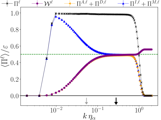
Figure 10: Scale-filtered fluxes for the kinetic and magnetic energy, normalized by the mean total energy dissipation rate $\varepsilon=\varepsilon_{u}+\varepsilon_{b}$, as a function of the adimensional parameter $k\eta_{\alpha}=\pi\eta_{\alpha}/\ell$. The p.d.f.s shown in figures 11–13 are calculated for the value of $k\eta_{\alpha}$ indicated by the thick (black) arrow, while the thin (grey) arrow denotes the value of $k\eta_{\alpha}$ used to calculate the p.d.f.s shown in sec. 4. Also shown is the kinetic–magnetic energy conversion term $\cal{W}^{\ell}$. The green dashed horizontal line corresponds to the $y$-axis value of $0.5$. The errorbars, although not fully visible, indicate one standard error.

Figure 10 displays the net kinetic energy flux, $\Pi^{I,\ell}+\Pi^{M,\ell}$, and the net magnetic energy flux, $\Pi^{A,\ell}+\Pi^{D,\ell}$, obtained using the Fourier filter and dataset A1. In essence it is a rearrangement of fig. 2. An equipartition region is evident for $0.2\lesssim k\eta_{\alpha}\lesssim 0.6$, where the magnetic and kinetic energy subfluxes reach approximately $50\%$ of the total energy flux, as indicated by the green dashed line. See Bian & Aluie (2019) for discussion of this feature. Moreover, this equipartition region is also the region where the conversion term ${\cal W}^{\ell}$ of eq. (7) saturates and becomes scale-independent.

Figure 11 displays energy (sub)fluxes for MHD dataset A1, for the filter scale $k\eta_{\alpha}=0.27$. Comparing these figures to those presented in section 4 it is apparent that the p.d.f.s in the equipartition region have fluctuations that are some three times larger. Recall that the p.d.f.s in figures 4, 7, and 9, were calculated for the larger scale $k\eta_{\alpha}=5.4\times 10^{-2}$. As we progress further into the inertial range the p.d.f.s develop even broader tails (not shown).

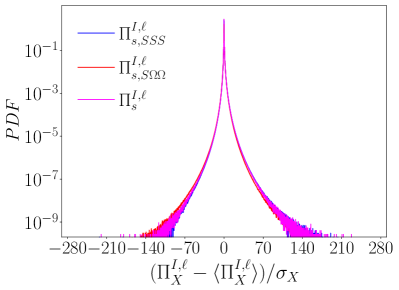
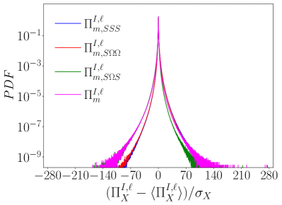
Figure 11: Standardised p.d.f.s of Inertial subfluxes $\Pi^{I,\ell}_{X}$ at $k\eta=0.27$, where $X$ represents the subflux identifier. Left: single-scale fluxes; right: multi-scale fluxes.

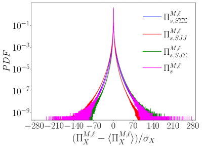
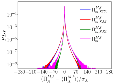
Figure 12: As for figure 11 for the Maxwell energy fluxes, $\Pi^{M,\ell}_{X}$.

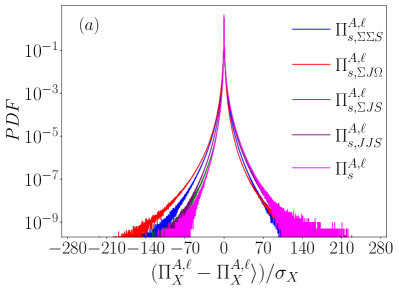
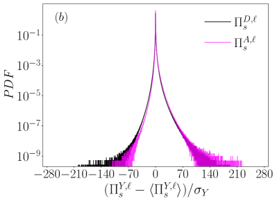
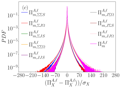
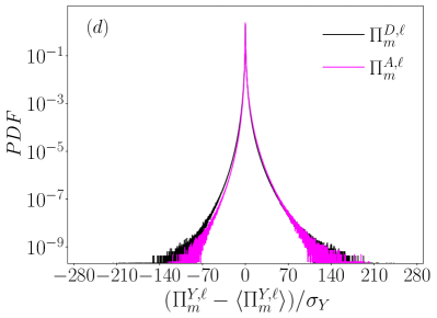
Figure 13: Standardised p.d.f.s. at $k\eta_{\alpha}=0.27$. (a) single-scale Advection subfluxes $\Pi^{A,\ell}_{s,X}$, where $X$ represents the subflux identifier. (b) single-scale net fluxes for the Dynamo and Advection terms, respectively $\Pi^{D,\ell}_{s}$ and $\Pi^{A,\ell}_{s}$, where $Y=D$ or $A$ identifies the term. The subflux $\Pi_{s}^{A,\ell}$ is shown in both panels. (c),(d) p.d.f.s of multi-scale Advection and Dynamo subfluxes, respectively.

Appendix E Subfluxes definitions

In this section we provide the definitions of all the subfluxes appearing in the decomposition of the MHD energy fluxes. As highlighted in sec. 3, for the subfluxes $\Pi^{I}_{s,S\Omega S}$, $\Pi^{I}_{m,S\Omega S}$ and $\Pi^{M}_{s,SJ\Sigma}$, $\Pi^{M}_{m,SJ\Sigma}$ there is an extra factor of two that arises from the symmetry of the corresponding SGS stress tensors. Because in eqs.(6) and (7) the fluxes appear with the same leading signs, both the Maxwell and the Dynamo subfluxes in the definition below acquires an additional minus sign.

E.1 Inertial

The following subfluxes are identical to the hydrodynamic counterpart from Johnson (2020, 2021).

$$\Pi^{I,\ell}_{s,SSS}=-\ell^{2}\,\mathrm{Tr}\left\{{\big{(}\overline{\bm{S}}^{\ell}\big{)}^{t}\,\overline{\bm{S}}^{\ell}\big{(}\overline{\bm{S}}^{\ell}\big{)}^{t}}\right\}$$ (71)

$$\Pi^{I,\ell}_{m,SSS}=-\int_{0}^{\ell^{2}}\!\!\mathrm{d}\theta\,\mathrm{Tr}\left\{{\big{(}\overline{\bm{S}}^{\ell}\big{)}^{t}\Big{(}\overline{\overline{\bm{S}}^{\sqrt{\theta}}\big{(}\overline{\bm{S}}^{\sqrt{\theta}}\big{)}^{t}\,}^{\phi}-\overline{\overline{\bm{S}}^{\sqrt{\theta}}\,}^{\phi}\;\overline{\big{(}\overline{\bm{S}}^{\sqrt{\theta}}\big{)}^{\!t}\,}^{\phi}\Big{)}}\right\}$$ (72)

$$\Pi^{I,\ell}_{s,S\Omega\Omega}=-\ell^{2}\,\mathrm{Tr}\left\{{\big{(}\overline{\bm{S}}^{\ell}\big{)}^{t}\,\overline{\bm{\Omega}}^{\ell}\big{(}\overline{\bm{\Omega}}^{\ell}\big{)}^{t}}\right\}$$ (73)

$$\Pi^{I,\ell}_{m,S\Omega\Omega}=-\int_{0}^{\ell^{2}}\!\!\mathrm{d}\theta\,\mathrm{Tr}\left\{{\big{(}\overline{\bm{S}}^{\ell}\big{)}^{t}\Big{(}\overline{\overline{\bm{\Omega}}^{\sqrt{\theta}}\big{(}\overline{\bm{\Omega}}^{\sqrt{\theta}}\big{)}^{t}\,}^{\phi}-\overline{\overline{\bm{\Omega}}^{\sqrt{\theta}}\,}^{\phi}\;\overline{\big{(}\overline{\bm{\Omega}}^{\sqrt{\theta}}\big{)}^{\!t}\,}^{\phi}\Big{)}}\right\}$$ (74)

$$\Pi^{I,\ell}_{s,S\Omega S}=-2\ell^{2}\,\mathrm{Tr}\left\{{\big{(}\overline{\bm{S}}^{\ell}\big{)}^{t}\,\overline{\bm{\Omega}}^{\ell}\big{(}\overline{\bm{S}}^{\ell}\big{)}^{t}}\right\}\equiv 0$$ (75)

$$\Pi^{I,\ell}_{m,S\Omega S}=-2\int_{0}^{\ell^{2}}\!\!\mathrm{d}\theta\,\mathrm{Tr}\left\{{\big{(}\overline{\bm{S}}^{\ell}\big{)}^{t}\Big{(}\overline{\overline{\bm{\Omega}}^{\sqrt{\theta}}\big{(}\overline{\bm{S}}^{\sqrt{\theta}}\big{)}^{t}\,}^{\phi}-\overline{\overline{\bm{\Omega}}^{\sqrt{\theta}}\,}^{\phi}\;\overline{\big{(}\overline{\bm{S}}^{\sqrt{\theta}}\big{)}^{\!t}\,}^{\phi}\Big{)}}\right\}$$ (76)

E.2 Maxwell

$$\Pi^{M,\ell}_{s,S\Sigma\Sigma}=\ell^{2}\,\mathrm{Tr}\left\{{\big{(}\overline{\bm{S}}^{\ell}\big{)}^{t}\,\overline{\bm{\Sigma}}^{\ell}\big{(}\overline{\bm{\Sigma}}^{\ell}\big{)}^{t}}\right\}$$ (77)

$$\Pi^{M,\ell}_{m,S\Sigma\Sigma}=\int_{0}^{\ell^{2}}\!\!\mathrm{d}\theta\,\mathrm{Tr}\left\{{\big{(}\overline{\bm{S}}^{\ell}\big{)}^{t}\Big{(}\overline{\overline{\bm{\Sigma}}^{\sqrt{\theta}}\big{(}\overline{\bm{\Sigma}}^{\sqrt{\theta}}\big{)}^{t}\,}^{\phi}-\overline{\overline{\bm{\Sigma}}^{\sqrt{\theta}}\,}^{\phi}\;\overline{\big{(}\overline{\bm{\Sigma}}^{\sqrt{\theta}}\big{)}^{\!t}\,}^{\phi}\Big{)}}\right\}$$ (78)

$$\Pi^{M,\ell}_{s,SJJ}=\ell^{2}\,\mathrm{Tr}\left\{{\big{(}\overline{\bm{S}}^{\ell}\big{)}^{t}\,\overline{\bm{J}}^{\ell}\big{(}\overline{\bm{J}}^{\ell}\big{)}^{t}}\right\}$$ (79)

$$\Pi^{M,\ell}_{m,SJJ}=\int_{0}^{\ell^{2}}\!\!\mathrm{d}\theta\,\mathrm{Tr}\left\{{\big{(}\overline{\bm{S}}^{\ell}\big{)}^{t}\Big{(}\overline{\overline{\bm{J}}^{\sqrt{\theta}}\big{(}\overline{\bm{J}}^{\sqrt{\theta}}\big{)}^{t}\,}^{\phi}-\overline{\overline{\bm{J}}^{\sqrt{\theta}}\,}^{\phi}\;\overline{\big{(}\overline{\bm{J}}^{\sqrt{\theta}}\big{)}^{\!t}\,}^{\phi}\Big{)}}\right\}$$ (80)

$$\Pi^{M,\ell}_{s,SJ\Sigma}=2\ell^{2}\,\mathrm{Tr}\left\{{\big{(}\overline{\bm{S}}^{\ell}\big{)}^{t}\,\overline{\bm{J}}^{\ell}\big{(}\overline{\bm{\Sigma}}^{\ell}\big{)}^{t}}\right\}$$ (81)

$$\Pi^{M,\ell}_{m,SJ\Sigma}=2\int_{0}^{\ell^{2}}\!\!\mathrm{d}\theta\,\mathrm{Tr}\left\{{\big{(}\overline{\bm{S}}^{\ell}\big{)}^{t}\Big{(}\overline{\overline{\bm{J}}^{\sqrt{\theta}}\big{(}\overline{\bm{\Sigma}}^{\sqrt{\theta}}\big{)}^{t}\,}^{\phi}-\overline{\overline{\bm{J}}^{\sqrt{\theta}}\,}^{\phi}\;\overline{\big{(}\overline{\bm{\Sigma}}^{\sqrt{\theta}}\big{)}^{\!t}\,}^{\phi}\Big{)}}\right\}$$ (82)

E.3 Advection

$$\Pi^{A,\ell}_{s,\Sigma\Sigma S}=-\ell^{2}\,\mathrm{Tr}\left\{{\big{(}\overline{\bm{\Sigma}}^{\ell}\big{)}^{t}\,\overline{\bm{\Sigma}}^{\ell}\big{(}\overline{\bm{S}}^{\ell}\big{)}^{t}}\right\}$$ (83)

$$\Pi^{A,\ell}_{m,\Sigma\Sigma S}=\;-\;\int_{0}^{\ell^{2}}\mathrm{d}\theta\,\mathrm{Tr}\left\{{\big{(}\overline{\bm{\Sigma}}^{\ell}\big{)}^{t}\Big{(}\overline{\overline{\bm{\Sigma}}^{\sqrt{\theta}}\big{(}\overline{\bm{S}}^{\sqrt{\theta}}\big{)}^{t}\,}^{\phi}-\overline{\overline{\bm{\Sigma}}^{\sqrt{\theta}}\,}^{\phi}\;\overline{\big{(}\overline{\bm{\Sigma}}^{\sqrt{\theta}}\big{)}^{\!t}\,}^{\phi}\Big{)}}\right\}$$ (84)

$$\Pi^{A,\ell}_{s,\Sigma JS}=-\ell^{2}\,\mathrm{Tr}\left\{{\big{(}\overline{\bm{\Sigma}}^{\ell}\big{)}^{t}\,\overline{\bm{J}}^{\ell}\big{(}\overline{\bm{S}}^{\ell}\big{)}^{t}}\right\}$$ (85)

$$\Pi^{A,\ell}_{m,\Sigma JS}=\;-\;\int_{0}^{\ell^{2}}\mathrm{d}\theta\,\mathrm{Tr}\left\{{\big{(}\overline{\bm{\Sigma}}^{\ell}\big{)}^{t}\Big{(}\overline{\overline{\bm{J}}^{\sqrt{\theta}}\big{(}\overline{\bm{S}}^{\sqrt{\theta}}\big{)}^{t}\,}^{\phi}-\overline{\overline{\bm{J}}^{\sqrt{\theta}}\,}^{\phi}\;\overline{\big{(}\overline{\bm{S}}^{\sqrt{\theta}}\big{)}^{\!t}\,}^{\phi}\Big{)}}\right\}$$ (86)

$$\Pi^{A,\ell}_{s,\Sigma\Sigma\Omega}=-\ell^{2}\,\mathrm{Tr}\left\{{\big{(}\overline{\bm{\Sigma}}^{\ell}\big{)}^{t}\,\overline{\bm{\Sigma}}^{\ell}\big{(}\overline{\bm{\Omega}}^{\ell}\big{)}^{t}}\right\}\equiv 0$$ (87)

$$\Pi^{A,\ell}_{m,\Sigma\Sigma\Omega}=\;-\;\int_{0}^{\ell^{2}}\mathrm{d}\theta\,\mathrm{Tr}\left\{{\big{(}\overline{\bm{\Sigma}}^{\ell}\big{)}^{t}\Big{(}\overline{\overline{\bm{\Sigma}}^{\sqrt{\theta}}\big{(}\overline{\bm{\Omega}}^{\sqrt{\theta}}\big{)}^{t}\,}^{\phi}-\overline{\overline{\bm{\Sigma}}^{\sqrt{\theta}}\,}^{\phi}\;\overline{\big{(}\overline{\bm{\Omega}}^{\sqrt{\theta}}\big{)}^{\!t}\,}^{\phi}\Big{)}}\right\}$$ (88)

$$\Pi^{A,\ell}_{s,\Sigma J\Omega}=-\ell^{2}\,\mathrm{Tr}\left\{{\big{(}\overline{\bm{\Sigma}}^{\ell}\big{)}^{t}\,\overline{\bm{J}}^{\ell}\big{(}\overline{\bm{\Omega}}^{\ell}\big{)}^{t}}\right\}$$ (89)

$$\Pi^{A,\ell}_{m,\Sigma J\Omega}=\;-\;\int_{0}^{\ell^{2}}\mathrm{d}\theta\,\mathrm{Tr}\left\{{\big{(}\overline{\bm{\Sigma}}^{\ell}\big{)}^{t}\Big{(}\overline{\overline{\bm{J}}^{\sqrt{\theta}}\big{(}\overline{\bm{\Omega}}^{\sqrt{\theta}}\big{)}^{t}\,}^{\phi}-\overline{\overline{\bm{J}}^{\sqrt{\theta}}\,}^{\phi}\;\overline{\big{(}\overline{\bm{\Omega}}^{\sqrt{\theta}}\big{)}^{\!t}\,}^{\phi}\Big{)}}\right\}$$ (90)

$$\Pi^{A,\ell}_{s,J\Sigma S}=-\ell^{2}\,\mathrm{Tr}\left\{{\big{(}\overline{\bm{J}}^{\ell}\big{)}^{t}\,\overline{\bm{\Sigma}}^{\ell}\big{(}\overline{\bm{S}}^{\ell}\big{)}^{t}}\right\}$$ (91)

$$\Pi^{A,\ell}_{m,J\Sigma S}=\;-\;\int_{0}^{\ell^{2}}\mathrm{d}\theta\,\mathrm{Tr}\left\{{\big{(}\overline{\bm{J}}^{\ell}\big{)}^{t}\Big{(}\overline{\overline{\bm{\Sigma}}^{\sqrt{\theta}}\big{(}\overline{\bm{S}}^{\sqrt{\theta}}\big{)}^{t}\,}^{\phi}-\overline{\overline{\bm{\Sigma}}^{\sqrt{\theta}}\,}^{\phi}\;\overline{\big{(}\overline{\bm{S}}^{\sqrt{\theta}}\big{)}^{\!t}\,}^{\phi}\Big{)}}\right\}$$ (92)

$$\Pi^{A,\ell}_{s,J\Sigma\Omega}=-\ell^{2}\,\mathrm{Tr}\left\{{\big{(}\overline{\bm{J}}^{\ell}\big{)}^{t}\,\overline{\bm{\Sigma}}^{\ell}\big{(}\overline{\bm{\Omega}}^{\ell}\big{)}^{t}}\right\}$$ (93)

$$\Pi^{A,\ell}_{m,J\Sigma\Omega}=\;-\;\int_{0}^{\ell^{2}}\mathrm{d}\theta\,\mathrm{Tr}\left\{{\big{(}\overline{\bm{J}}^{\ell}\big{)}^{t}\Big{(}\overline{\overline{\bm{\Sigma}}^{\sqrt{\theta}}\big{(}\overline{\bm{\Omega}}^{\sqrt{\theta}}\big{)}^{t}\,}^{\phi}-\overline{\overline{\bm{\Sigma}}^{\sqrt{\theta}}\,}^{\phi}\;\overline{\big{(}\overline{\bm{\Omega}}^{\sqrt{\theta}}\big{)}^{\!t}\,}^{\phi}\Big{)}}\right\}$$ (94)

$$\Pi^{A,\ell}_{s,JJS}=-\ell^{2}\,\mathrm{Tr}\left\{{\big{(}\overline{\bm{J}}^{\ell}\big{)}^{t}\,\overline{\bm{J}}^{\ell}\big{(}\overline{\bm{S}}^{\ell}\big{)}^{t}}\right\}$$ (95)

$$\Pi^{A,\ell}_{m,JJS}=\;-\;\int_{0}^{\ell^{2}}\mathrm{d}\theta\,\mathrm{Tr}\left\{{\big{(}\overline{\bm{J}}^{\ell}\big{)}^{t}\Big{(}\overline{\overline{\bm{J}}^{\sqrt{\theta}}\big{(}\overline{\bm{S}}^{\sqrt{\theta}}\big{)}^{t}\,}^{\phi}-\overline{\overline{\bm{J}}^{\sqrt{\theta}}\,}^{\phi}\;\overline{\big{(}\overline{\bm{S}}^{\sqrt{\theta}}\big{)}^{\!t}\,}^{\phi}\Big{)}}\right\}$$ (96)

$$\Pi^{A,\ell}_{s,JJ\Omega}=-\ell^{2}\,\mathrm{Tr}\left\{{\big{(}\overline{\bm{J}}^{\ell}\big{)}^{t}\,\overline{\bm{J}}^{\ell}\big{(}\overline{\bm{\Omega}}^{\ell}\big{)}^{t}}\right\}\equiv 0$$ (97)

$$\Pi^{A,\ell}_{m,JJ\Omega}=\;-\;\int_{0}^{\ell^{2}}\mathrm{d}\theta\,\mathrm{Tr}\left\{{\big{(}\overline{\bm{J}}^{\ell}\big{)}^{t}\Big{(}\overline{\overline{\bm{J}}^{\sqrt{\theta}}\big{(}\overline{\bm{\Omega}}^{\sqrt{\theta}}\big{)}^{t}\,}^{\phi}-\overline{\overline{\bm{J}}^{\sqrt{\theta}}\,}^{\phi}\;\overline{\big{(}\overline{\bm{\Omega}}^{\sqrt{\theta}}\big{)}^{\!t}\,}^{\phi}\Big{)}}\right\}$$ (98)

E.4 Dynamo

$$\Pi^{D,\ell}_{s,\Sigma S\Sigma}=\ell^{2}\,\mathrm{Tr}\left\{{\big{(}\overline{\bm{\Sigma}}^{\ell}\big{)}^{t}\,\overline{\bm{S}}^{\ell}\big{(}\overline{\bm{\Sigma}}^{\ell}\big{)}^{t}}\right\}$$ (99)

$$\Pi^{D,\ell}_{m,\Sigma S\Sigma}=\;\;\int_{0}^{\ell^{2}}\mathrm{d}\theta\,\mathrm{Tr}\left\{{\big{(}\overline{\bm{\Sigma}}^{\ell}\big{)}^{t}\Big{(}\overline{\overline{\bm{S}}^{\sqrt{\theta}}\big{(}\overline{\bm{\Sigma}}^{\sqrt{\theta}}\big{)}^{t}\,}^{\phi}-\overline{\overline{\bm{S}}^{\sqrt{\theta}}\,}^{\phi}\;\overline{\big{(}\overline{\bm{\Sigma}}^{\sqrt{\theta}}\big{)}^{\!t}\,}^{\phi}\Big{)}}\right\}$$ (100)

$$\Pi^{D,\ell}_{s,\Sigma\Omega\Sigma}=\ell^{2}\,\mathrm{Tr}\left\{{\big{(}\overline{\bm{\Sigma}}^{\ell}\big{)}^{t}\,\overline{\bm{\Omega}}^{\ell}\big{(}\overline{\bm{\Sigma}}^{\ell}\big{)}^{t}}\right\}\equiv 0$$ (101)

$$\Pi^{D,\ell}_{m,\Sigma\Omega\Sigma}=\;\;\int_{0}^{\ell^{2}}\mathrm{d}\theta\,\mathrm{Tr}\left\{{\big{(}\overline{\bm{\Sigma}}^{\ell}\big{)}^{t}\Big{(}\overline{\overline{\bm{\Omega}}^{\sqrt{\theta}}\big{(}\overline{\bm{\Sigma}}^{\sqrt{\theta}}\big{)}^{t}\,}^{\phi}-\overline{\overline{\bm{\Omega}}^{\sqrt{\theta}}\,}^{\phi}\;\overline{\big{(}\overline{\bm{\Sigma}}^{\sqrt{\theta}}\big{)}^{\!t}\,}^{\phi}\Big{)}}\right\}$$ (102)

$$\Pi^{D,\ell}_{s,\Sigma SJ}=\ell^{2}\,\mathrm{Tr}\left\{{\big{(}\overline{\bm{\Sigma}}^{\ell}\big{)}^{t}\,\overline{\bm{S}}^{\ell}\big{(}\overline{\bm{J}}^{\ell}\big{)}^{t}}\right\}$$ (103)

$$\Pi^{D,\ell}_{m,\Sigma SJ}=\;\;\int_{0}^{\ell^{2}}\mathrm{d}\theta\,\mathrm{Tr}\left\{{\big{(}\overline{\bm{\Sigma}}^{\ell}\big{)}^{t}\Big{(}\overline{\overline{\bm{S}}^{\sqrt{\theta}}\big{(}\overline{\bm{J}}^{\sqrt{\theta}}\big{)}^{t}\,}^{\phi}-\overline{\overline{\bm{S}}^{\sqrt{\theta}}\,}^{\phi}\;\overline{\big{(}\overline{\bm{J}}^{\sqrt{\theta}}\big{)}^{\!t}\,}^{\phi}\Big{)}}\right\}$$ (104)

$$\Pi^{D,\ell}_{s,\Sigma\Omega J}=\ell^{2}\,\mathrm{Tr}\left\{{\big{(}\overline{\bm{\Sigma}}^{\ell}\big{)}^{t}\,\overline{\bm{\Omega}}^{\ell}\big{(}\overline{\bm{J}}^{\ell}\big{)}^{t}}\right\}$$ (105)

$$\Pi^{D,\ell}_{m,\Sigma\Omega J}=\;\;\int_{0}^{\ell^{2}}\mathrm{d}\theta\,\mathrm{Tr}\left\{{\big{(}\overline{\bm{\Sigma}}^{\ell}\big{)}^{t}\Big{(}\overline{\overline{\bm{\Omega}}^{\sqrt{\theta}}\big{(}\overline{\bm{J}}^{\sqrt{\theta}}\big{)}^{t}\,}^{\phi}-\overline{\overline{\bm{\Omega}}^{\sqrt{\theta}}\,}^{\phi}\;\overline{\big{(}\overline{\bm{J}}^{\sqrt{\theta}}\big{)}^{\!t}\,}^{\phi}\Big{)}}\right\}$$ (106)

$$\Pi^{D,\ell}_{s,JS\Sigma}=\ell^{2}\,\mathrm{Tr}\left\{{\big{(}\overline{\bm{J}}^{\ell}\big{)}^{t}\,\overline{\bm{S}}^{\ell}\big{(}\overline{\bm{\Sigma}}^{\ell}\big{)}^{t}}\right\}$$ (107)

$$\Pi^{D,\ell}_{m,JS\Sigma}=\;\;\int_{0}^{\ell^{2}}\mathrm{d}\theta\,\mathrm{Tr}\left\{{\big{(}\overline{\bm{J}}^{\ell}\big{)}^{t}\Big{(}\overline{\overline{\bm{S}}^{\sqrt{\theta}}\big{(}\overline{\bm{\Sigma}}^{\sqrt{\theta}}\big{)}^{t}\,}^{\phi}-\overline{\overline{\bm{S}}^{\sqrt{\theta}}\,}^{\phi}\;\overline{\big{(}\overline{\bm{\Sigma}}^{\sqrt{\theta}}\big{)}^{\!t}\,}^{\phi}\Big{)}}\right\}$$ (108)

$$\Pi^{D,\ell}_{s,J\Omega\Sigma}=\ell^{2}\,\mathrm{Tr}\left\{{\big{(}\overline{\bm{J}}^{\ell}\big{)}^{t}\,\overline{\bm{\Omega}}^{\ell}\big{(}\overline{\bm{\Sigma}}^{\ell}\big{)}^{t}}\right\}$$ (109)

$$\Pi^{D,\ell}_{m,J\Omega\Sigma}=\;\;\int_{0}^{\ell^{2}}\mathrm{d}\theta\,\mathrm{Tr}\left\{{\big{(}\overline{\bm{J}}^{\ell}\big{)}^{t}\Big{(}\overline{\overline{\bm{\Omega}}^{\sqrt{\theta}}\big{(}\overline{\bm{\Sigma}}^{\sqrt{\theta}}\big{)}^{t}\,}^{\phi}-\overline{\overline{\bm{\Omega}}^{\sqrt{\theta}}\,}^{\phi}\;\overline{\big{(}\overline{\bm{\Sigma}}^{\sqrt{\theta}}\big{)}^{\!t}\,}^{\phi}\Big{)}}\right\}$$ (110)

$$\Pi^{D,\ell}_{s,JSJ}=\ell^{2}\,\mathrm{Tr}\left\{{\big{(}\overline{\bm{J}}^{\ell}\big{)}^{t}\,\overline{\bm{S}}^{\ell}\big{(}\overline{\bm{J}}^{\ell}\big{)}^{t}}\right\}$$ (111)

$$\Pi^{D,\ell}_{m,JSJ}=\;\;\int_{0}^{\ell^{2}}\mathrm{d}\theta\,\mathrm{Tr}\left\{{\big{(}\overline{\bm{J}}^{\ell}\big{)}^{t}\Big{(}\overline{\overline{\bm{S}}^{\sqrt{\theta}}\big{(}\overline{\bm{J}}^{\sqrt{\theta}}\big{)}^{t}\,}^{\phi}-\overline{\overline{\bm{S}}^{\sqrt{\theta}}\,}^{\phi}\;\overline{\big{(}\overline{\bm{J}}^{\sqrt{\theta}}\big{)}^{\!t}\,}^{\phi}\Big{)}}\right\}$$ (112)

$$\Pi^{D,\ell}_{s,J\Omega J}=\ell^{2}\,\mathrm{Tr}\left\{{\big{(}\overline{\bm{J}}^{\ell}\big{)}^{t}\,\overline{\bm{\Omega}}^{\ell}\big{(}\overline{\bm{J}}^{\ell}\big{)}^{t}}\right\}\equiv 0$$ (113)

$$\Pi^{D,\ell}_{m,J\Omega J}=\;\;\int_{0}^{\ell^{2}}\mathrm{d}\theta\,\mathrm{Tr}\left\{{\big{(}\overline{\bm{J}}^{\ell}\big{)}^{t}\Big{(}\overline{\overline{\bm{\Omega}}^{\sqrt{\theta}}\big{(}\overline{\bm{J}}^{\sqrt{\theta}}\big{)}^{t}\,}^{\phi}-\overline{\overline{\bm{\Omega}}^{\sqrt{\theta}}\,}^{\phi}\;\overline{\big{(}\overline{\bm{J}}^{\sqrt{\theta}}\big{)}^{\!t}\,}^{\phi}\Big{)}}\right\}$$ (114)

References

- Adkins et al. (2022) Adkins, T., Schekochihin, A. A., Ivanov, P. G. & Roach, C. M. 2022 Electromagnetic instabilities and plasma turbulence driven by electron-temperature gradient. J. Plasma Phys. 88, 905880410.
- Alexakis (2013) Alexakis, A. 2013 Large-scale magnetic fields in magnetohydrodynamic turbulence. Phys. Rev. Lett. 110.
- Alexakis (2017) Alexakis, A. 2017 Helically decomposed turbulence. J. Fluid Mech. 812, 752–770.
- Alexakis & Biferale (2018) Alexakis, A. & Biferale, L. 2018 Cascades and transitions in turbulent flows. Phys. Rep. 767-769, 1–101.
- Alexakis & Chibbaro (2022) Alexakis, A. & Chibbaro, S. 2022 Local fluxes in magnetohydrodynamic turbulence. J. Plasma Phys. 88 (5), 905880515.
- Aluie (2017) Aluie, H. 2017 Coarse-grained incompressible magnetohydrodynamics: analyzing the turbulent cascades. New J. Phys. 19, 025008.
- Aluie & Eyink (2010) Aluie, H. & Eyink, G. L. 2010 Scale locality of magnetohydrodynamic turbulence. Phys. Rev. Lett. 104.
- Batchelor (1970) Batchelor, G. K. 1970 The Theory of Homogeneous Turbulence. Cambridge, UK: Cambridge University Press.
- Beresnyak (2019) Beresnyak, A. 2019 MHD turbulence. Living Reviews in Computational Astrophysics 5 (1), 2.
- Betchov (1956) Betchov, R. 1956 An inequality concerning the production of vorticity in isotropic turbulence. J. Fluid Mech. 1, 497.
- Bian & Aluie (2019) Bian, X. & Aluie, H. 2019 Decoupled cascades of kinetic and magnetic energy in magnetohydrodynamic turbulence. Phys. Rev. Lett. 122, 135101.
- Biskamp (2003) Biskamp, D. 2003 Magnetohydrodynamic Turbulence. Cambridge, UK: Cambridge University Press.
- Borue & Orszag (1995) Borue, V. & Orszag, S. A. 1995 Self-similiar decay of three-dimensional homogeneous turbulence with hyperviscosity. Phys. Rev. E 51, R856.
- Borue & Orszag (1998) Borue, V. & Orszag, S. A. 1998 Local energy flux and subgrid-scale statistics in three-dimensional turbulence. J. Fluid Mech. 366, 1–31.
- Brandenburg et al. (2012) Brandenburg, A., Sokoloff, D. & Subramanian, K. 2012 Current status of turbulent dynamo theory. Space Sci. Rev. 169, 123–157.
- Bruno & Carbone (2013) Bruno, R. & Carbone, V. 2013 The solar wind as a turbulence laboratory. Living Rev. Solar Phys. 10.
- Buzzicotti et al. (2018) Buzzicotti, M., Aluie, H., Biferale, L & Linkmann, M. 2018 Energy transfer in turbulence under rotation. Phys. Rev. Fluids 3, 034802.
- Canuto et al. (1988) Canuto, C., Hussaini, M. Y., Quarteroni, A. & Zang, T. A. 1988 Spectral Methods in Fluid Mechanics. New York: Springer–Verlag.
- Capocci et al. (2023) Capocci, D., Johnson, P. L., Oughton, S., Biferale, L. & Linkmann, M. 2023 New exact Betchov-like relation for the helicity flux in homogeneous turbulence. J. Fluid Mech. 963, R1.
- Chen et al. (2006) Chen, S., Ecke, R. E., Eyink, G. L., Rivera, M., Wan, M. & Xiao, Z. 2006 Physical mechanism of the two-dimensional inverse energy cascade. Phys. Rev. Lett. 96, 084502.
- Chernyshov et al. (2010) Chernyshov, A. A., Karelsky, K. V. & Petrosyan, A. S. 2010 Forced turbulence in large-eddy simulation of compressible magnetohydrodynamic turbulence. Phys. Plasmas 17 (10), 102307.
- Clark et al. (1979) Clark, R. A., Ferziger, J. H. & Reynolds, W. C. 1979 Evaluation of subgrid-scale models using an accurately simulated turbulent flow. J. Fluid Mech. 91 (1), 1–16.
- Davidson (1999) Davidson, P. A. 1999 Magnetohydrodynamics in materials processing. Annu. Rev. Fluid Mech. 31, 273–300.
- Davidson (2016) Davidson, P. A. 2016 Introduction to Magnetohydrodynamics. Cambridge University Press.
- Donzis et al. (2008) Donzis, D. A., Yeung, P. K. & Sreenivasan, K. R. 2008 Dissipation and enstrophy in isotropic turbulence: Resolution effects and scaling in direct numerical simulations. Phys. Fluids 20.
- Eyink (2006) Eyink, G. L. 2006 Multi-scale gradient expansion of the turbulent stress tensor. J. Fluid Mech. 549, 159–190.
- Freidberg (2007) Freidberg, J. P. 2007 Plasma physics and fusion energy. Cambridge University Press.
- Germano (1992) Germano, M. 1992 Turbulence — the filtering approach. J. Fluid Mech. 238, 325–336.
- Goldreich & Sridhar (1995) Goldreich, P. & Sridhar, S. 1995 Toward a theory of interstellar turbulence: II. Strong Alfvénic turbulence. Astrophys. J. 438, 763–775.
- Goldreich & Sridhar (1997) Goldreich, P. & Sridhar, S. 1997 Magnetohydrodynamic turbulence revisited. Astrophys. J. 485, 680–688.
- Grete et al. (2016) Grete, P., Vlaykov, D. G., Schmidt, W. & Schleicher, D. R. G. 2016 A nonlinear structural subgrid-scale closure for compressible MHD. II. A priori comparison on turbulence simulation data. Phys. Plasmas 23.
- Hamba & Tsuchiya (2010) Hamba, F. & Tsuchiya, M. 2010 Cross-helicity dynamo effect in magnetohydrodynamic turbulent channel flow. Phys. Plasmas 17 (1), 012301.
- Ivanov et al. (2022) Ivanov, P. G., Schekochihin, A.A. & Dorland, W. 2022 Dimits transition in three-dimensional ion-temperature-gradient turbulence. Journal of Plasma Physics 88 (5), 905880506.
- Ivanov et al. (2020) Ivanov, P. G., Schekochihin, A. A., Dorland, W., Field, A. R. & Parra, F. I. 2020 Zonally dominated dynamics and dimits threshold in curvature-driven itg turbulence. J. Plasma Phys. 86 (5), 855860502.
- Jadhav & Chandy (2021) Jadhav, K. & Chandy, A. J. 2021 Large eddy simulations of high-magnetic Reynolds number magnetohydrodynamic turbulence for non-helical and helical initial conditions: A study of two sub-grid scale models. Phys. Fluids 33 (8), 085131.
- Jadhav & Chandy (2023) Jadhav, K. & Chandy, A. J. 2023 Large eddy simulations of inhomogeneous high-magnetic Reynolds number magnetohydrodynamic flows. Phys. Fluids 35 (7), 075109.
- Johnson (2020) Johnson, P. L. 2020 Energy transfer from large to small scales in turbulence by multiscale nonlinear strain and vorticity interactions. Phys. Rev. Lett. 124, 104501.
- Johnson (2021) Johnson, P. L. 2021 On the role of vorticity stretching and strain self-amplification in the turbulence energy cascade. J. Fluid Mech. 922, A3.
- Johnson (2022) Johnson, P. L. 2022 A physics-inspired alternative to spatial filtering for large-eddy simulations of turbulent flows. J. Fluid Mech. 934, A30.
- Jones (2011) Jones, C. A. 2011 Planetary magnetic fields and fluid dynamos. Annu. Rev. Fluid Mech. 43, 583–614.
- Kessar et al. (2016) Kessar, M., Balarac, G. & Plunian, F. 2016 The effect of subgrid-scale models on grid-scale/subgrid-scale energy transfers in large-eddy simulation of incompressible magnetohydrodynamic turbulence. Phys. Plasmas 23 (10).
- Kraichnan (1976) Kraichnan, R. H. 1976 Eddy viscosity in two and three dimensions. J. Atmos. Sci. 33, 1521–1536.
- Leonard (1975) Leonard, A. 1975 Energy cascade in large-eddy simulations of turbulent fluid flows. In Adv. Geophys., , vol. 18, pp. 237–248. Elsevier.
- Lessinnes et al. (2011) Lessinnes, T., Plunian, F., Stepanov, R. & Carati, D. 2011 Dissipation scales of kinetic helicities in turbulence. Phys. Fluids 23.
- Linkmann et al. (2018) Linkmann, M., Buzzicotti, M. & Biferale, L. 2018 Multi-scale properties of large eddy simulations: correlations between resolved-scale velocity-field increments and subgrid-scale quantities. J. Turb. 19, 493–527.
- Linkmann et al. (2015) Linkmann, M. F., Berera, A., McComb, W. D. & McKay, M. E. 2015 Nonuniversality and finite dissipation in decaying magnetohydrodynamic turbulence. Phys. Rev. Lett. 114, 235001.
- Matthaeus (2021) Matthaeus, W. H. 2021 Turbulence in space plasmas: Who needs it? Phys. Plasmas 28 (3), 032306.
- Matthaeus et al. (2015) Matthaeus, W. H., Wan, M., Servidio, S., Greco, A., Osman, K. T., Oughton, S. & Dmitruk, P. 2015 Intermittency, nonlinear dynamics, and dissipation in the solar wind and astrophysical plasmas. Phil. Trans. R. Soc. A 373.
- Meneveau & Katz (2000) Meneveau, C. & Katz, J. 2000 Scale-invariance and turbulence models for large-eddy simulation. Ann. Rev. Fluid Mech. 32, 1–32.
- Meyrand et al. (2015) Meyrand, R., Kiyani, K. H. & Galtier, S. 2015 Weak magnetohydrodynamic turbulence and intermittency. J. Fluid Mech. 770, R1.
- Miesch et al. (2015) Miesch, M., Matthaeus, W., Brandenburg, A., Petrosyan, A., Pouquet, A., Cambon, C., Jenko, F., Uzdensky, D., Stone, J., Tobias, S., Toomre, J. & Velli, M. 2015 Large-eddy simulations of magnetohydrodynamic turbulence in heliophysics and astrophysics. Space Sci. Rev. 194, 97–137.
- Mininni & Pouquet (2009) Mininni, P. D. & Pouquet, A. 2009 Finite dissipation and intermittency in magnetohydrodynamics. Phys. Rev. E 80, 025401.
- Miura & Araki (2012) Miura, H. & Araki, K. 2012 Coarse-graining study of homogeneous and isotropic hall magnetohydrodynamics turbulence. Plasma Physics and Controlled Fusion 55.
- Miura et al. (2016) Miura, H., Araki, K. & Hamba, F. 2016 Hall effects and sug-gird-scale modelling in magnetohydrodynamic turbulence simulations. J. Comp. Phys. 316, 385–395.
- Miura et al. (2017) Miura, H., Hamba, F. & Ito, A. 2017 Two-fluid sub-grid-scale viscosity in nonlinear simulation of ballooning modes in a heliotron device. Nuclear Fusion 57, 076034.
- Müller & Carati (2002a) Müller, W.-C. & Carati, D. 2002a Dynamic gradient-diffusion subgrid models for incompressible magnetohydrodynamic turbulence. Phys. Plasmas 9 (3), 824–834.
- Müller & Carati (2002b) Müller, W.-C. & Carati, D. 2002b Dynamic gradient-diffusion subgrid models for incompressible magnetohydrodynamic turbulence. Phys. Plasmas 9 (3), 824–834.
- Offermans et al. (2018) Offermans, G. P., Biferale, L., Buzzicotti, M. & Linkmann, M. 2018 A priori study of the subgrid energy transfers for small-scale dynamo in kinematic and saturation regimes. Phys. Plasmas 25 (12), 122307.
- Oughton et al. (1994) Oughton, S., Priest, E. R. & Matthaeus, W. H. 1994 The influence of a mean magnetic field on three-dimensional MHD turbulence. J. Fluid Mech. 280, 95–117.
- Patterson & Orszag (1971) Patterson, G. S. & Orszag, S. A. 1971 Spectral calculations of isotropic turbulence: Efficient removal of aliasing interactions. Phys. Fluids 14, 2538–2541.
- Petrosyan et al. (2010) Petrosyan, A., Balogh, A., Goldstein, M. L., Léorat, J., Marsch, E., Petrovay, K., Roberts, B., von Steiger, R. & Vial, J. C. 2010 Turbulence in the solar atmosphere and solar wind. Space Sci. Rev. p. 117.
- Plunian et al. (2013) Plunian, F., Stepanov, R. & Frick, P. 2013 Shell models of magnetohydrodynamic turbulence. Phys. Rep. 523 (1), 1–60, shell Models of Magnetohydrodynamic Turbulence.
- Pope (2000) Pope, S. B. 2000 Turbulent Flows. Cambridge, UK: Cambridge University Press.
- Rodriguez Imazio et al. (2013) Rodriguez Imazio, P., Martin, L. N., Dmitruk, P. & Mininni, P. D. 2013 Intermittency in Hall-magnetohydrodynamics with a strong guide field. Phys. Plasmas 20, 052506.
- Sahoo et al. (2011) Sahoo, G., Perlekar, P. & Pandit, R. 2011 Systematics of the magnetic-Prandtl-number dependence of homogeneous, isotropic magnetohydrodynamic turbulence. New J. Phys. 13, 013036.
- Salem et al. (2009) Salem, C., Mangeney, A., Bale, S. D. & Veltri, P. 2009 Solar wind magnetohydrodynamics turbulence: Anomalous scaling and role of intermittency. Astrophys. J. 702, 537–553.
- Schekochihin (2022) Schekochihin, A. A. 2022 MHD turbulence: A biased review. J. Plasma Phys. 88 (5), 155880501.
- Schmidt (2015) Schmidt, W. 2015 Large eddy simulations in astrophysics. Living Rev. Comput. Astrophys. 1, 2.
- Shebalin et al. (1983) Shebalin, J. V., Matthaeus, W. H. & Montgomery, D. 1983 Anisotropy in MHD turbulence due to a mean magnetic field. J. Plasma Phys. 29, 525–547.
- Spyksma et al. (2012) Spyksma, K., Magcalas, M. & Campbell, N. 2012 Quantifying effects of hyperviscosity on isotropic turbulence. Phys. Fluids 24.
- Tobias & Cattaneo (2013) Tobias, S. M. & Cattaneo, F. 2013 Shear-driven dynamo waves at high magnetic Reynolds number. Nature 497, 463–465.
- Vela-Martín (2022) Vela-Martín, A. 2022 Subgrid-scale models of isotropic turbulence need not produce energy backscatter. J. Fluid Mech. 937, A14.
- Veltri (1999) Veltri, P. 1999 MHD turbulence in the solar wind: Self-similarity, intermittency and coherent structures. Plasma Phys. Controlled Fusion 41, A787–A795.
- Vlaykov et al. (2016) Vlaykov, D. G., Grete, P., Schmidt, W. & Schleicher, D. R. G. 2016 A nonlinear structural subgrid-scale closure for compressible MHD. I. Derivation and energy dissipation properties. Phys. Plasmas 23.
- Vreman et al. (1996) Vreman, B., Geurts, B. & Kuerten, H. 1996 Large-eddy simulation of the turbulent mixing layer using the clark model. Theor. Compu. Fluid Dyn. 8, 309–324.
- Vreman et al. (1997) Vreman, B., Geurts, B. & Kuerten, H. 1997 Large-eddy simulation of the turbulent mixing layer. J. Fluid Mech. 339, 357–390.
- Waleffe (1993) Waleffe, F. 1993 Inertial transfers in the helical decomposition. Phys. Fluids A 5, 667.
- Wan et al. (2012) Wan, M., Osman, K. T., Matthaeus, W. H. & Oughton, S. 2012 Investigation of intermittency in magnetohydrodynamics and solar wind turbulence: Scale-dependent kurtosis. Astrophys. J. 744, 171.
- Wan et al. (2010) Wan, M., Oughton, S., Servidio, S. & Matthaeus, W. H. 2010 On the accuracy of simulations of turbulence. Phys. Plasmas 17.
- Weiss & Proctor (2014) Weiss, N. O. & Proctor, M. R. E. 2014 Magnetoconvection. Cambridge University Press.
- Yang et al. (2023) Yang, P.-F., Zhou, Z. D., Xu, H. & He, G. W. 2023 Strain self-amplification is larger than vortex stretching due to an invariant relation of filtered velocity gradients. J. Fluid Mech. 955, A15.
- Yang et al. (2021) Yang, Y., Linkmann, M., Biferale, L. & Wan, M. 2021 Effects of forcing mechanisms on the multiscale properties of magnetohydrodynamics. Astrophys. J. 909 (2), 175.
- Yoshimatsu et al. (2011) Yoshimatsu, K., Schneider, K., Okamoto, N., Kawahara, Y. & Farge, M. 2011 Intermittency and geometrical statistics of three-dimensional homogeneous magnetohydrodynamic turbulence: A wavelet viewpoint. Phys. Plasmas 18, 092304.
- Zhou et al. (2004) Zhou, Y., Matthaeus, W. H. & Dmitruk, P. 2004 Magnetohydrodynamic turbulence and time scales in astrophysical and space plasmas. Rev. Mod. Phys. 76, 1015–1035.
- Zhou & Vahala (1991) Zhou, Y. & Vahala, G. 1991 Aspects of subgrid modelling and large-eddy simulation of magnetohydrodynamic turbulence. J. Plasma Phys. 45 (2), 239–249.