A geometric approach toconjugation-invariant random permutations

Abstract

We propose a new approach to conjugation-invariant random permutations. Namely, we explain how to construct uniform permutations in given conjugacy classes from certain point processes in the plane. This enables the use of geometric tools to study various statistics of such permutations. For their longest decreasing subsequences, we prove universality of the $2\sqrt{n}$ asymptotic. For Robinson–Schensted shapes, we prove universality of the Vershik–Kerov–Logan–Shepp limit shape, thus solving a conjecture of Kammoun. For the number of records, we establish a phase transition phenomenon as the number of fixed points grows. For pattern counts, we obtain an asymptotic normality result, partially answering a conjecture of Hamaker and Rhoades.

1 Introduction

1.1 Conjugation-invariant random permutations

We say that a random permutation $\tau$ of $[n]:=\{1,\dots,n\}$ is conjugation-invariant when for any fixed permutation $\rho$, the conjugate $\rho\circ\tau\circ\rho^{-1}$ follows the same law as $\tau$. Standard examples of conjugation-invariant permutations are uniformly random permutations, random involutions, Ewens random permutations [Ewe72], their generalizations [Kin78, Tsi00, BUV11], and many more.

An equivalent description of conjugation-invariance makes use of the cycle decomposition. Define the cycle type of $\tau$ as the sequence $t=(t_{1},t_{2},\dots,t_{n})$ where $t_{p}$ is the number of $p$-cycles in $\tau$. We also say that $t$ has size $\sum_{p=1}^{n}pt_{p}=n$ and that $\tau$ is $t$-cyclic. Since the cycle type is a total invariant for conjugation in the symmetric group, a random permutation $\tau$ is conjugation-invariant if and only if, when conditioned on its cycle type $t$, $\tau$ is a uniform $t$-cyclic permutation. Thus, studying conjugation-invariant random permutations often amounts to studying uniform permutations with given cycle types.

There are reasons to believe in universality phenomena for several statistics of conjugation-invariant permutations, with a dependence on the number of fixed points and sometimes $2$-cycles. Recent advances motivate this idea by generalizing asymptotic properties of uniformly random permutations to conjugation-invariant random permutations under certain hypotheses [Fér13, Kam18, FKL22, HR22]. The aim of this paper is to make further progress in this direction by introducing a “geometric” construction for random permutations in given conjugacy classes, see Section 1.2. This new point of view allows us to establish asymptotic results on the longest monotone subsequences, Robinson–Schensted shape, number of records, and pattern counts.

Longest monotone subsequences.

The maximum length of a monotone subsequence in a uniform permutation famously behaves as $2\sqrt{n}$ [VK77]. Baik and Rains [BR01] showed similar asymptotics for random involutions, with a dependence on the number of fixed points, and Kammoun [Kam18] proved that the $2\sqrt{n}$ asymptotic holds for conjugation-invariant permutations with few cycles. In Section 2.1 we extend these results to general conjugation-invariant random permutations for their longest decreasing subsequences. Longest increasing subsequences are harder to handle, and we only provide such asymptotics up to a multiplicative constant.

Robinson–Schensted shape.

The Robinson–Schensted shape of a uniform permutation converges, after suitable rescaling, to a limit curve [LS77, VK77]. Kammoun [Kam18] extended this result to conjugation-invariant permutations with few cycles, and conjectured that this assumption could be lifted. In Section 2.2 we provide a positive answer to this conjecture.

Records.

The numbers of records in uniform permutations are known to satisfy asymptotic normality. In Section 2.3 we prove a general limit theorem for the number of high records (or left-to-right maxima) in conjugation-invariant permutations, showcasing a phase transition as the number of fixed points grows. More precisely, the number of high records interpolates from logarithmic with Gaussian fluctuations to asymptotically Gamma, when the number of non-fixed points is of order $n/\sqrt{\log n}$. We also find the first order asymptotics of low records (or left-to-right minima), and their second order asymptotics in some cases.

Pattern counts.

Janson et al. [JNZ15] established asymptotic normality for all pattern counts in uniform permutations. Kammoun [Kam22] and Hamaker and Rhoades [HR22] extended this to conjugation-invariant permutations, under certain assumptions on their cycles. The authors of [HR22] conjectured that the (non-degenerate) asymptotic normality of pattern counts holds for all conjugation-invariant permutations, where the asymptotic variance depends on the numbers of fixed points and $2$-cycles. In Section 2.4 we partially answer this conjecture, by proving asymptotic normality for all conjugation-invariant permutations, and non-degeneracy in some cases.

1.2 A geometric construction

Let $\mathcal{P}=\{Z_{1},\dots,Z_{n}\}$ be a finite subset of $\mathbb{R}^{2}$ with no redundant x- or y-coordinates. Then we can define a permutation $\tau$ of $[n]$ by letting $\tau(i)=j$ when the $i$-th point from the left in $\mathcal{P}$ is $j$-th from the bottom. We write $\tau={\rm Perm}\left(\mathcal{P}\right)$ for this permutation; see Figure 1 for an example.

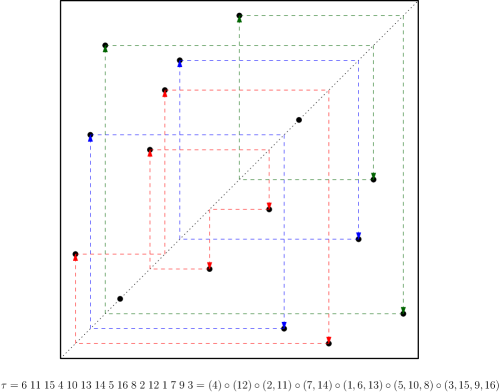
Figure 1: Representation of the geometric construction of a uniform $(2,2,2,1)$-cyclic permutation as in 1.1, written in one-line notation and in cycle product notation.

By considering adequate planar point processes $\mathcal{P}$, we may obtain random permutations $\tau$ with various laws: for instance if $Z_{1},\dots,Z_{n}$ are i.i.d. ${\rm Unif}\left([0,1]^{2}\right)$ variables then $\tau$ is uniformly random, and if we symmetrize this family with respect to the diagonal of $[0,1]^{2}$ then $\tau$ is a uniform involution of size $2n$ with no fixed point [BR01]. An asset of this point of view is that some properties of $\tau$ may be easier to derive directly from $\mathcal{P}$: see e.g. [AD95] for a study of increasing subsequences in uniform permutations, and [Kiw06] for the case of involutions. 1.1 generalizes the geometric construction of Baik and Rains for random involutions [BR01] to uniform permutations in any conjugacy class. Although simple, this lemma is fundamental to our analysis: general conjugation–invariant permutations do not benefit from the same valuable algebraic properties as uniform permutations or involutions, and our geometric construction bypasses this problem.

If $t$ is a cycle type of size $n$, define $\mathcal{V}_{t}:=\left\{\big{.}(p,k,l)\,:\,p\in[n],k\in[t_{p}],l\in[p]\right\}$. Using a family of i.i.d. uniform variables indexed by this set, we can construct a uniform $t$-cyclic permutation as follows. This is illustrated on Figure 1.

Lemma 1.1.

Let $t$ be a cycle type of size $n$. Let $\left(U_{p,k}^{l}\right)_{(p,k,l)\in\mathcal{V}_{t}}$ be a family of i.i.d. ${\rm Unif}\left([0,1]\right)$ random variables. For each $(p,k,l)\in\mathcal{V}_{t}$, write $Z_{p,k}^{l}:=\left(U_{p,k}^{l},U_{p,k}^{l+1}\right)$ where $l\!+\!1$ is taken modulo $p$, and set $\mathcal{P}:=\left\{Z_{p,k}^{l}:(p,k,l)\in\mathcal{V}_{t}\right\}$. Then $\tau:={\rm Perm}\left(\mathcal{P}\right)$ is a uniform $t$-cyclic permutation.

Proof.

The list of x-coordinates of $\mathcal{P}$ is the same as its list of y-coordinates, namely $\mathcal{U}=\left\{U_{p,k}^{l}\,:\,(p,k,l)\in\mathcal{V}_{t}\right\}$. Write $i_{p,k}^{l}\in[n]$ for the relative order of $U_{p,k}^{l}$ in $\cal U$, i.e. $U_{p,k}^{l}$ is the $i_{p,k}^{l}$-th lowest value in $\cal U$. Then the presence of $\left(U_{p,k}^{l},U_{p,k}^{l\!+\!1}\right)$ in $\mathcal{P}$ means that $\tau\left(i_{p,k}^{l}\right)=i_{p,k}^{l\!+\!1}$. Therefore $\tau$ is the product of cycles $\left(i_{p,k}^{1},\dots,i_{p,k}^{p}\right)$ for $p\in[n]$, $k\in[t_{p}]$. In other words, $\tau$ is obtained by writing the sequence $\left(i_{p,k}^{l}\right)_{(p,k,l)\in\mathcal{V}_{t}}$ with the lexicographic order on $(p,k,l)$, parenthesizing it according to the cycle type $t$, and interpreting this as a product of cycles. By standardization of the i.i.d. sequence $\left(U_{p,k}^{l}\right)_{(p,k,l)\in\mathcal{V}_{t}}$, the sequence $\left(i_{p,k}^{l}\right)_{(p,k,l)\in\mathcal{V}_{t}}$ is the one-line representation of a uniformly random permutation of $[n]$. From there, it is classical that $\tau$ is a uniform $t$-cyclic permutation. ∎

As we explain in Sections 2.1, 2.2 and 2.3, monotone subsequences and records of $\tau={\rm Perm}\left(\mathcal{P}\right)$ can be read directly on $\mathcal{P}$. This allows us to study these statistics of the permutation by investigating the behavior of the point process in certain regions of the plane. To this aim, a list of useful properties of the geometric construction may be found in Section 3. Regarding pattern counts, we rather use the “weak dependency” of points in $\mathcal{P}$ (see Section 2.4 for more details).

1.3 Notation

We denote by $\mathfrak{S}_{n}$ the set of permutations of $[n]$ and by $\Delta$ the diagonal of $[0,1]^{2}$. Throughout this paper we consider the standard partial order on $\mathbb{R}^{2}$ defined by $(x,y)\leq(x^{\prime},y^{\prime})$ when $x\leq x^{\prime}$ and $y\leq y^{\prime}$.

Let $t$ be a cycle type of size $n$. We say that $\mathcal{P}$ is a geometric construction of $t$ when $\mathcal{P}$ is constructed as in 1.1. We can decompose it into its cycles $\mathcal{P}=\bigcup_{p\in[n],k\in[t_{p}]}\mathcal{P}_{p,k}$ where $\mathcal{P}_{p,k}:=\left\{Z_{p,k}^{l}:l\in[p]\right\}$. We can also decompose it into $\mathcal{P}_{\Delta}:=\mathcal{P}\cap\Delta$ and $\check{\mathcal{P}}:=\mathcal{P}\setminus\Delta$, and we write $\check{t}:=(0,t_{2},t_{3},\dots,t_{n})$ for the cycle type of size $\check{n}:=n-t_{1}$ with no fixed point. It is straightforward to check that $\check{\mathcal{P}}$ is a geometric construction of $\check{t}$.

We define a “successor” operator $\mathfrak{s}:(p,k,l)\in\mathcal{V}_{t}\mapsto(p,k,l\!+\!1)\in\mathcal{V}_{t}$ where $l\!+\!1$ is taken modulo $p$, and a graph $\mathcal{L}_{t}:=(\mathcal{V}_{t},\mathcal{E}_{t})$ with vertice $\mathcal{V}_{t}$ and edges between $i$ and $\mathfrak{s}(i)$ for each $i\in\mathcal{V}_{t}$ (forgetting self-loops). We refer to $\mathcal{L}_{t}$ as the “dependency graph” associated with $t$. See Figure 2 for an example, and Section 7.1 for an explanation of this name.

Figure 2: The dependency graph $\mathcal{L}_{t}$ associated with the cycle type $t=(2,1,2,0,1)$.

Let $(a_{n})_{n\in\mathbb{N}}$ be a sequence of positive numbers. We say that a sequence of random variables $(X_{n})_{n\in\mathbb{N}}$ is a $\mathcal{O}_{\mathbf{P}}(a_{n})$ as $n\to\infty$ if

$$\sup_{n\in\mathbb{N}}\mathbf{P}\left(\left|X_{n}\right|>a_{n}M\right)\underset{M\to+\infty}{\longrightarrow}0.$$

Also, $(X_{n})_{n\in\mathbb{N}}$ is a $o_{\mathbf{P}}(a_{n})$ as $n\to\infty$ if $X_{n}/a_{n}\underset{n\to\infty}{\longrightarrow}0$ in probability. Finally, a sequence $(A_{n})_{n\in\mathbb{N}}$ of events happens with high probability (w.h.p.) as $n\to\infty$ if $\mathbf{P}\left(A_{n}\right)\underset{n\to\infty}{\longrightarrow}1$.

2 Results: universality and beyond

2.1 Longest monotone subsequences

Let $\tau$ be a permutation of $[n]$. An increasing subsequence of $\tau$ is a sequence of indices $i_{1}<\dots<i_{\ell}$ such that $\tau(i_{1})<\dots<\tau(i_{\ell})$, and the maximum length of an increasing subsequence of $\tau$ is denoted by $\mathrm{LIS}(\tau)$. We may define analogously $\mathrm{LDS}(\tau)$ as the maximum length of a decreasing subsequence of $\tau$.

The study of monotone subsequences in permutations has been an active and captivating field of research; see [Rom15] for an introduction. In particular when $\tau_{n}$ is uniformly random, the law of $\mathrm{LIS}(\tau_{n})$ (which is the same as that of $\mathrm{LDS}(\tau_{n})$ in this case) is now well understood: it behaves asymptotically as $2\sqrt{n}$ [VK77], satisfies a large deviation principle [DZ99], and admits Tracy–Widom fluctuations of order $n^{1/6}$ [BDJ99].

One might expect these results to mostly hold when the law of $\tau_{n}$ is invariant by conjugation. The first advance on this question was obtained by Baik and Rains, who studied random involutions [BR01]. More recently, Kammoun [Kam18, Kam23] and Guionnet [GK23] could settle the case of conjugation-invariant random permutations with few cycles. Here we start by stating first order asymptotic results and concentration inequalities for the longest decreasing subsequences of uniform permutations with given cycle types and no fixed points.

Theorem 2.1.

For any $\delta>0$ there exists $c_{\delta}>0$ such that the following holds. For each $n$, let $t^{(n)}$ be a cycle type of size $n$ such that $t_{1}^{(n)}=0$ and let $\tau_{n}$ be a uniform $t^{(n)}$-cyclic permutation. Then:

$$\mathbf{P}\left(\frac{1}{\sqrt{n}}\mathrm{LDS}(\tau_{n})<2(1-\delta)\right)\leq\exp\left(\big{.}-c_{\delta}n\right)\quad\text{;}\quad\mathbf{P}\left(\frac{1}{\sqrt{n}}\mathrm{LDS}(\tau_{n})>2(1+\delta)\right)\leq\exp\left(-c_{\delta}\sqrt{n}\right).$$

In particular $\frac{1}{\sqrt{n}}\mathrm{LDS}(\tau_{n})\underset{n\to\infty}{\longrightarrow}2$ in probability and in $L^{q}$ for all $q\geq 1$.

It is not difficult to add fixed points in the previous theorem, and to consider random cycle types instead of deterministic ones. This yields the following corollary.

Corollary 2.2.

For any $\delta>0$ there exists $c_{\delta}>0$ such that the following holds. Let $(\tau_{n})_{n}$ be a sequence of conjugation-invariant random permutations, where $\tau_{n}$ has size $n$ and (random) cycle type $t^{(n)}$. Then for any $n$:

$$\left\{\begin{array}[]{ll}\mathbf{P}\left(\mathrm{LDS}(\tau_{n})<2(1-\delta)\sqrt{n-t_{1}^{(n)}}\right)\leq\mathbb{E}\left[\exp\left(\big{.}-c_{\delta}\left(n-t_{1}^{(n)}\right)\right)\right];\vspace{.5em}\\ \mathbf{P}\left(\mathrm{LDS}(\tau_{n})>2(1+\delta)\sqrt{n-t_{1}^{(n)}}\right)\leq\mathbb{E}\left[\exp\left(-c_{\delta}\sqrt{n-t_{1}^{(n)}}\right)\right].\end{array}\right.$$

In particular if $n-t_{1}^{(n)}\to\infty$ in probability then $\frac{1}{\sqrt{n-t_{1}^{(n)}}}\mathrm{LDS}(\tau_{n})\to 2$ in probability and in $L^{q}$ for all $q\geq 1$.

Remark 1.

In comparison with [Kam18, Theorem 1.2] and its variants in [Kam23], 2.2 does not require any hypothesis on the number of cycles. Our results can in particular be applied to random permutations with cycle weights, some of which have a lot of cycles [BUV11, EU14], and to central virtual permutations, some of which have a macroscopic number of fixed points [Tsi00]. A similar observation can be made for all of the results presented in this paper.

Although increasing and decreasing subsequences share the same distribution in uniformly random permutations, this fact does not hold for conjugation-invariant random permutations. The study of increasing subsequences in this context is trickier, and we were only able to derive their first order asymptotics up to a multiplicative constant. As before, we start by stating our result for uniform permutations with given cycle types and no fixed points, and then we generalize it to all conjugation-invariant permutations.

Proposition 2.3.

For any $\delta>0$ there exists $c_{\delta}>0$ such that the following holds. For each $n$, let $t^{(n)}$ be a cycle type of size $n$ such that $t_{1}^{(n)}=0$ and let $\tau_{n}$ be a uniform $t^{(n)}$-cyclic permutation. Then:

$$\mathbf{P}\left(\frac{1}{\sqrt{n}}\mathrm{LIS}(\tau_{n})<2(1-\delta)\right)\leq\exp\left(-c_{\delta}n\right)\quad\text{ ; }\quad\mathbf{P}\left(\frac{1}{\sqrt{n}}\mathrm{LIS}(\tau_{n})>2(1+\delta)\sqrt{3}\right)\leq\exp\left(-c_{\delta}\sqrt{n}\right).$$

Corollary 2.4.

For any $\delta>0$ there exists $c_{\delta}>0$ such that the following holds. Let $(\tau_{n})_{n}$ be a sequence of conjugation-invariant random permutations, where $\tau_{n}$ has size $n$ and (random) cycle type $t^{(n)}$. Then for any $n$:

$$\left\{\begin{array}[]{ll}\mathbf{P}\left(\big{.}\mathrm{LIS}(\tau_{n})<2(1-\delta)\sqrt{n}\right)\leq\exp\left(-c_{\delta}n\right);\vspace{.5em}\\ \mathbf{P}\left(\mathrm{LIS}(\tau_{n})>t_{1}^{(n)}+2(1+\delta)\sqrt{3\left(n-t_{1}^{(n)}\right)}\right)\leq\mathbb{E}\left[\exp\left(-c_{\delta}\sqrt{n-t_{1}^{(n)}}\right)\right].\end{array}\right.$$

In particular if $\frac{1}{\sqrt{n}}t_{1}^{(n)}\to\alpha\geq 0$ in probability then $\frac{1}{\sqrt{n}}\mathrm{LIS}(\tau_{n})$ is asymptotically bounded between $2$ and $\alpha+2\sqrt{3}$ in probability.

Let us briefly explain the techniques used to prove the results of this section. Deuschel and Zeitouni [DZ95] studied the first order asymptotics of longest monotone subsequences in ${\rm Perm}\left(Z_{1},\dots,Z_{n}\right)$, where $Z_{1},\dots,Z_{n}$ are i.i.d. under certain probability densities on $[0,1]^{2}$ (such random permutations are called locally uniform in [Sjö23]). This is made possible by the following key observation: increasing and decreasing subsequences of $\tau={\rm Perm}\left(\mathcal{P}\right)$ correspond to up-right and down-right paths of points in $\mathcal{P}$. The authors of [DZ95] then slice the unit square into small rectangles in which the points are almost uniformly distributed, so that they may locally apply the result of [VK77], and finally stitch these local paths of points into one global path. When studying uniform permutations in given conjugacy classes, the same method can be adapted to the geometric construction of 1.1.

Finally, we state a reasonable conjecture in the direction of 2.3 and 2.4. It was already established for random involutions in [BR01], and for conjugation-invariant random permutations satisfying certain cycle constraints in [Kam18, Theorem 1.2] and [Kam23, Theorem 3].

Conjecture 2.5.

Let $(\tau_{n})_{n}$ be a sequence of conjugation-invariant random permutations, where $\tau_{n}$ has size $n$ and (random) cycle type $t^{(n)}$. Suppose that $t_{1}^{(n)}/\sqrt{n}\rightarrow 0$ in probability. Then

$$\frac{1}{\sqrt{n}}\mathrm{LIS}(\tau_{n})\underset{n\to\infty}{\longrightarrow}2$$

in probability.

Remark 2.

Baik and Rains actually proved [BR01, Theorems 3.2 and 3.4] that if $\tau_{n}$ is a uniform $t^{(n)}$-cyclic permutation where $t^{(n)}~{}=~{}\left(t_{1}^{(n)},t_{2}^{(n)},0,\dots\right)$ satisfies $t_{1}^{(n)}/\sqrt{n}\to\alpha\geq 0$, i.e. if $\tau_{n}$ is a uniform involution with $\alpha\sqrt{n}+o(\sqrt{n})$ fixed points, then

$$\frac{1}{\sqrt{n}}\mathrm{LIS}(\tau_{n})\underset{n\to\infty}{\longrightarrow}\left\{\begin{array}[]{ll}2&\text{if }\alpha\leq 1\vspace{.5em}\\ \alpha+\frac{1}{\alpha}&\text{if }\alpha\geq 1\end{array}\right.$$

in probability. We could expect the same first order asymptotics for any sequence of conjugation-invariant random permutations such that $t_{1}^{(n)}/\sqrt{n}\to\alpha$ in probability. However we chose not to include this refinement of 2.5 in its statement, as it might be more speculative.

The results of this section are proved in Section 4.

2.2 Robinson–Schensted shape

Let $\tau$ be a permutation of $[n]$. If $x\geq 0$, we call $x$-decrasing subsequence any union of $\lfloor x\rfloor$ individually decreasing subsequences, and we define $\mathrm{LDS}_{x}(\tau)$ as the maximal size of an $x$-decreasing subsequence of $\tau$.

The study of $x$-decreasing subsequences in permutations is partly motivated by their fundamental link with the Robinson–Schensted correspondence. This is a one-to-one correspondence between permutations and pairs of standard Young tableaux with the same shape. This shape, which is a Young diagram, is called the RS shape of the permutation: it appears in several domains, such as integrable probability or representation theory. A well-known theorem of Greene [Gre74] states that for any integer $k$, the number of boxes in the first $k$ columns of the RS shape of $\tau$ equals $\mathrm{LDS}_{k}(\tau)$. Equivalently, the length of the $k$-th column equals $\mathrm{LDS}_{k}(\tau)-\mathrm{LDS}_{k\!-\!1}(\tau)$. A similar connection can be made between increasing subsequences of $\tau$ and the row lengths of its RS shape.

Historically, studying the asymptotics of $\mathrm{LIS}(\tau_{n})$ and $\mathrm{LDS}(\tau_{n})$ when $\tau_{n}$ is uniformly random actually required finding the asymptotics of its entire RS shape. The law of this shape is known as the Plancherel measure, for which Vershik and Kerov and simultaneously Logan and Shepp established the following.

Theorem 2.6 ([LS77, VK77]).

For each $n$, let $\tau_{n}$ be a uniformly random permutation of $[n]$. Then there exists an explicit nondecreasing, concave function $F_{\mathrm{LSKV}}:\mathbb{R}_{+}\to\mathbb{R}_{+}$ such that for each $r\geq 0$:

$$\frac{1}{n}\mathrm{LDS}_{r\sqrt{n}}(\tau_{n})\underset{n\to\infty}{\longrightarrow}F_{\mathrm{LSKV}}(r)$$

in probability.

According to Greene’s theorem, $F_{\mathrm{LSKV}}(r)$ thus describes the asymptotic proportion of boxes in the first $\lfloor r\sqrt{n}\rfloor$ columns of the RS shape of $\tau_{n}$, and the derivative of $F_{\mathrm{LSKV}}$ describes the limit curve of this shape.

A classical property of the Robinson–Schensted correspondence is that it induces a bijection between involutions and (single) standard Young tableaux. If $(\tau_{n})$ is a sequence of uniformly random involutions, the proofs of [LS77] and [VK77] can then be adapted to show that Theorem 2.6 still holds (see e.g. Equation (24) in [Mel11] and the discussion below). More generally if $(\tau_{n})$ is a sequence of conjugation-invariant random permutations, Kammoun proved that Theorem 2.6 still holds under the assumption that the number of cycles in $\tau_{n}$ is sublinear [Kam18, Theorem 1.8]. He later conjectured that this assumption could be lifted, provided we take into account the proportion of fixed points [Kam23, Conjectures 6 and 7]. The main difficulty is that none of the previous approaches (via hook-length formula [LS77], representation theory [IO02, Mel11], coupling [Kam18]…) work in this wider setting. Here, using our geometric construction, we solve this conjecture.

Theorem 2.7.

For each $n$, let $t^{(n)}$ be a cycle type of size $n$ with no fixed point and let $\tau_{n}$ be a uniform $t^{(n)}$-cyclic permutation. Then for each $r\geq 0$:

$$\frac{1}{n}\mathrm{LDS}_{r\sqrt{n}}(\tau_{n})\underset{n\to\infty}{\longrightarrow}F_{\mathrm{LSKV}}(r)$$

in probability.

Corollary 2.8.

Let $(\tau_{n})_{n}$ be a sequence of conjugation-invariant random permutations, where $\tau_{n}$ has size $n$ and (random) cycle type $t^{(n)}$. Suppose that $n-t_{1}^{(n)}\to\infty$ in probability. Then for each $r\geq 0$:

$$\frac{1}{n-t_{1}^{(n)}}\mathrm{LDS}_{r\sqrt{n-t_{1}^{(n)}}}(\tau_{n})\underset{n\to\infty}{\longrightarrow}F_{\mathrm{LSKV}}(r)$$

in probability.

Let us briefly discuss the strategy of proof. As in Section 2.1, $k$-decreasing subsequences of $\tau={\rm Perm}\left(\mathcal{P}\right)$ have a nice visual interpretation: they correspond to unions of $k$ down-right paths in $\mathcal{P}$. In the continuity of [DZ95], where the longest monotone subsequences of locally uniform permutations were studied with geometric tools, Sjöstrand [Sjö23] recently studied the limit RS shape of locally uniform permutations using more advanced analysis. His approach broadly consisted in computing the “score” associated with a bundle of decreasing curves, by decomposing the unit square into small regions where the sampling density is almost constant and the curves are almost parallel. In 3.3 we show that the points of our geometric construction, when restricted to any rectangle outside the diagonal of the unit square, are i.i.d. uniform. This simple fact is at the basis of how we apply and adapt the results and methods of [Sjö23].

The results of this section are proved in Section 5.

2.3 Records

Let $\tau$ be a permutation of $[n]$. We say that a position $i\in[n]$ is a high record (or left-to-right maximum) for $\tau$ if for any $j<i$, we have $\tau(j)<\tau(i)$. We say that it is a low record (or left-to-right minimum) for $\tau$ if for any $j<i$, we have $\tau(j)>\tau(i)$. We denote by $\mathrm{rec}^{\uparrow}\left(\tau\right)$ and $\mathrm{rec}^{\downarrow}\left(\tau\right)$ the numbers of high and low recods in $\tau$, respectively. Records and their many variants are standard statistics in enumerative combinatorics.

The numbers of low and high records in uniformly random permutations are well understood: thanks to a classical bijection they follow the same law as the number of cycles (see e.g. [ABNP16, Section 1.2]), and this yields the following asymptotic normality (found e.g. in [ABT03, Equation (1.31)]).

Theorem 2.9.

For each $n$, let $\tau_{n}$ be a uniformly random permutation of $[n]$. Then we have the following convergence in distribution:

$$\frac{\mathrm{rec}^{\uparrow}\left(\tau_{n}\right)-\log n}{\sqrt{\log n}}\underset{n\to\infty}{\longrightarrow}{\cal N}\left(0,1\right).$$

The same holds for $\mathrm{rec}^{\downarrow}\left(\tau_{n}\right)$.

Records can be interpreted nicely when the permutation is obtained from a family of points in the plane. If $\tau={\rm Perm}\left(\mathcal{P}\right)$, a point $Z=(X,Y)\in\mathcal{P}$ corresponds to a high record in $\tau$ when no other point lies in its up-left corner $[0,X]\times[Y,1]$. Similarly, $Z$ corresponds to a low record in $\tau$ when no other point lies in its down-left corner $[0,X]\times[0,Y]$. We write $\mathrm{rec}^{\uparrow}\left(\mathcal{P}\right)$ and $\mathrm{rec}^{\downarrow}\left(\mathcal{P}\right)$ as shortcuts for $\mathrm{rec}^{\uparrow}\left({\rm Perm}\left(\mathcal{P}\right)\right)$ and $\mathrm{rec}^{\downarrow}\left({\rm Perm}\left(\mathcal{P}\right)\right)$.

There is no more link between the numbers of cycles and records in conjugation-invariant permutations, but the geometric construction enables a new approach. We prove a limit theorem for the number of high records, showcasing a phase transition as the number of fixed points grows. First recall that, for $n\in\mathbb{N}^{*}$ and $\lambda>0$, the $\mathrm{Gamma}\left(n,\lambda\right)$ distribution is defined as the $n$-th convolution power of the ${\rm Exp}\left(\lambda\right)$ distribution. By convention, $\mathrm{Gamma}\left(n,+\infty\right)$ is the a.s. null distribution.

Theorem 2.10.

For each $n$, let $t^{(n)}$ be a cycle type of size $n$ and let $\tau_{n}$ be a uniform $t^{(n)}$-cyclic permutation. Write $\check{n}:=n-t_{1}^{(n)}$ for the number of non-fixed points. Suppose that $\check{n}\underset{n\to\infty}{\longrightarrow}\infty$ and that

$$\frac{\check{n}}{n/\sqrt{\log n}}\underset{n\to\infty}{\longrightarrow}\alpha$$

for some $\alpha\in[0,\infty]$. Then we have the following convergence in distribution:

$$\frac{\mathrm{rec}^{\uparrow}\left(\tau_{n}\right)-\log\left(\check{n}\right)}{t_{1}^{(n)}/\check{n}+\sqrt{\log\left(\check{n}\right)}}\underset{n\to\infty}{\longrightarrow}\frac{\alpha}{\alpha+1}Y+\frac{1}{\alpha+1}\Gamma_{2}$$

where $Y$ and $\Gamma_{2}$ are independent ${\cal N}\left(0,1\right)$ and $\mathrm{Gamma}\left(2,1\right)$ random variables. In particular if $\check{n}=\omega\left(\frac{n}{\sqrt{\log n}}\right)$ as $n\to\infty$ then:

$$\frac{\mathrm{rec}^{\uparrow}\left(\tau_{n}\right)-\log n}{\sqrt{\log n}}\underset{n\to\infty}{\longrightarrow}{\cal N}\left(0,1\right).$$

Similar to the case of monotone subsequences, the study of low records in conjugation-invariant random permutations differs from that of high records. This asymmetry is already seen in some regimes for the first order asymptotics, as shown in the following theorem.

Theorem 2.11.

For each $n$, let $t^{(n)}$ be a cycle type of size $n$ and let $\tau_{n}$ be a uniform $t^{(n)}$-cyclic permutation.

1. If $t_{1}^{(n)}=\mathcal{O}\left(\sqrt{n}\right)$ then we have the following convergence in probability:

   $$\frac{\mathrm{rec}^{\downarrow}\left(\tau_{n}\right)}{\log n}\underset{n\to\infty}{\longrightarrow}1.$$

2. If $\sqrt{n}\ll t_{1}^{(n)}\ll n$, i.e. $\sqrt{n}=o\left(t_{1}^{(n)}\right)$ and $t_{1}^{(n)}=o(n)$, then we have the following convergence in probability:

   $$\frac{\mathrm{rec}^{\downarrow}\left(\tau_{n}\right)}{\log n-\log t_{1}^{(n)}}\underset{n\to\infty}{\longrightarrow}2.$$

3. If $t_{1}^{(n)}=\Theta\left(n\right)$ then $\mathrm{rec}^{\downarrow}\left(\tau_{n}\right)=\mathcal{O}_{\mathbf{P}}(1)$.

We could not compute fluctuations for the number of low records in general. To simplify the analysis, we restrict ourselves to products of $2$-cycles and products of $3$-cycles, for which exhibit different fluctuations.

Proposition 2.12.

For each $n$, let $t^{(n)}$ be a cycle type of size $n$ such that $t_{1}^{(n)}=\mathcal{O}\left(\sqrt{n}\right)$, and let $\tau_{n}$ be a uniform $t^{(n)}$-cyclic permutation.

1. Suppose that $t_{1}^{(n)}+2t_{2}^{(n)}=n$. Then we have the following convergence in distribution:

   $$\frac{\mathrm{rec}^{\downarrow}\left(\tau_{n}\right)-\log n}{\sqrt{\log n}}\underset{n\to\infty}{\longrightarrow}{\cal N}\left(0,2\right).$$

2. Suppose that $t_{1}^{(n)}+3t_{3}^{(n)}=n$. Then we have the following convergence in distribution:

   $$\frac{\mathrm{rec}^{\downarrow}\left(\tau_{n}\right)-\log n}{\sqrt{\log n}}\underset{n\to\infty}{\longrightarrow}{\cal N}\left(0,1\right).$$

It would be interesting to find the interpolation between the two items of 2.12. However this would notably require understanding the interaction between $2$-cycles and other cycles, and its effect on the law of low records, which seems difficult to grasp.

Remark 3.

As in Corollaries 2.2, 2.4, 2.8 and 2.16, the results of this section remain true if $(\tau_{n})$ is a sequence of conjugation-invariant random permutations and the hypotheses hold in probability.

The results of this section are proved in Section 6.

2.4 Pattern counts

Let $\tau\in\mathfrak{S}_{n}$ and $I=\{i_{1}<\dots<i_{r}\}$ be a subset of $[n]$. We may define a permutation $\pi\in\mathfrak{S}_{r}$ by the following rule: for any $j,k\in[r]$, $\pi(j)>\pi(k)$ if and only if $\tau(i_{j})>\tau(i_{k})$. We write $\mathrm{pat}(I,\tau)$ for this permutation, and say that this is the pattern induced by $\tau$ on $I$.

Permutation patterns are a natural notion of substructures for permutations, and as such they have attracted a lot of interest. A central question is that of pattern counts: given a permutation $\pi$ of $[r]$, how many subsets of $\tau$ induce $\pi$ as a pattern? In other words, we are interested in the statistic

$$X_{\pi}(\tau):=\sum_{I\in\binom{[n]}{r}}\mathbf{1}_{\mathrm{pat}(I,\tau)=\pi}$$

where $\binom{[n]}{r}$ denotes the subsets of $[n]$ of size $r$. For example, $X_{2\,1}(\tau)$ counts the number of inversions in $\tau$, and $X_{1\,2\,\dots\,r}(\tau)$ counts the number of increasing subsequences of length $r$ in $\tau$.

Pattern counts in uniformly random permutations are known to be asymptotically normal since the works of Bóna for monotone patterns [Bón10], and later Janson et al. for all patterns:

Theorem 2.13 ([JNZ15]).

For each $n$, let $\tau_{n}$ be a uniformly random permutation of $[n]$. Then for any $r\in\mathbb{N}^{*}$:

$$\left(\frac{X_{\pi}(\tau_{n})-\binom{n}{r}\frac{1}{r!}}{n^{r-1/2}}\right)_{\pi\in\mathfrak{S}_{r}}\underset{n\to\infty}{\longrightarrow}{\cal N}\left(0,\Sigma\right)$$

for some matrix $\Sigma$, of rank $(r\!-\!1)^{2}$ and such that $\Sigma_{\pi,\pi}>0$ for all $\pi\in\mathfrak{S}_{r}$ if $r\geq 2$.

The convergence result in this theorem can be established via the method of dependency graphs. To prove non-degeneracy, i.e. that $\Sigma_{\pi,\pi}$ is positive, Bóna was able to find a lower bound for the variance of $X_{\pi}$ by expressing it in terms of covariances, while the authors of [JNZ15] used the method of U-statistics.

In [Fér13], Féray established a central limit theorem for pattern counts in Ewens random permutations, and conjectured its non-degeneracy. Kammoun [Kam22, Proposition 31] and Hamaker and Rhoades [HR22, Theorem 8.8] could generalize the non-degenerate asymptotic normality of Theorem 2.13 to conjugation-invariant permutations, under certain conditions on their cycles. It was conjectured in [HR22, Problem 9.9] that those conditions could be lifted, and that the asymptotic variance would only depend on the proportions of fixed points and $2$-cycles.

Here, using the geometric construction of 1.1, we extend the convergence of Theorem 2.13 to most conjugation-invariant permutations. If $\tau_{n}$ is a uniform $t$-cyclic permutation then we can write, for any $\pi\in\mathfrak{S}_{r}$:

$$X_{\pi}(\tau_{n})=\sum_{I\in\binom{\mathcal{V}_{t}}{r}}\mathbf{1}_{{\rm Perm}\left(Z_{i},i\in I\right)=\pi}$$ (1)

with the notation of Section 1.2. Thanks to the dependency graph $\mathcal{L}_{t}$ defined in Section 1.3, we derive a limit theorem for $X_{\pi}(\tau_{n})$. More precisely, Stein’s method yields explicit bounds on the speed of convergence. In the following, we denote by $d_{K}$ the Kolmogorov distance between two probability distributions.

Theorem 2.14.

Let $Y\sim{\cal N}\left(0,1\right)$. For each $n$, let $t^{(n)}$ be a cycle type of size $n$ and $\tau_{n}$ be a uniform $t^{(n)}$-cyclic permutation. Fix $r\in\mathbb{N}^{*}$ and $\pi\in\mathfrak{S}_{r}$. Then for any $n$:

$$d_{K}\left(\frac{X_{\pi}(\tau_{n})-\mathbb{E}\left[X_{\pi}(\tau_{n})\right]}{\sqrt{\mathrm{Var}\left[X_{\pi}(\tau_{n})\right]}}\,,\,Y\right)\leq 42\frac{r}{(r\!-\!1)!^{2}}\frac{n^{2r-3/2}}{\mathrm{Var}\left[X_{\pi}(\tau_{n})\right]}+72\frac{r}{(r\!-\!1)!^{3}}\frac{n^{3r-2}}{\mathrm{Var}\left[X_{\pi}(\tau_{n})\right]^{3/2}}.$$

Furthermore if $\mathrm{Var}\left[X_{\pi}(\tau_{n})\right]=\sigma^{2}n^{2r-1}+o(n^{2r-1})$ for some $\sigma\geq 0$ as $n\to\infty$, then

$$\frac{X_{\pi}(\tau_{n})-\mathbb{E}\left[X_{\pi}(\tau_{n})\right]}{n^{r-1/2}}\underset{n\to\infty}{\longrightarrow}{\cal N}\left(0,\sigma^{2}\right)$$

in distribution, and if $\sigma>0$ then the previous distance is bounded by $\mathcal{O}(n^{-1/2})$.

Thanks to [HR22, Proposition 7.2 and Theorem 8.14], the condition $\mathrm{Var}\left[X_{\pi}(\tau_{n})\right]=\sigma^{2}n^{2r-1}+o(n^{2r-1})$ holds under the simple assumption that $t_{1}^{(n)}/n$ and $t_{2}^{(n)}/n$ converge. We may still want to find an explicit formula for $\sigma$, and to understand in which cases $\sigma>0$. For this we use the method of $U$-statistics developed by Hoeffding [Hoe48], as was done in [JNZ15]. Before stating our results, we need a few definitions.

Fix $r\in\mathbb{N}^{*}$ and $p_{1}\in[0,1]$. Then let $\hat{Z}_{1},\dots,\hat{Z}_{r}$ be i.i.d. variables distributed under $p_{1}\mathrm{Leb}_{\Delta}+(1\!-\!p_{1})\mathrm{Leb}_{[0,1]^{2}}$, where $\mathrm{Leb}_{\Delta}$ denotes the Lebesgue measure on the diagonal $\Delta$ of $[0,1]^{2}$. Define, for any $z\in[0,1]^{2}$:

$$\psi_{\pi}^{p_{1}}(z):=\mathbf{P}\left({\rm Perm}\left(\hat{Z}_{1},\dots,\hat{Z}_{r-1},z\right)=\pi\right)$$

and

$$\mu_{\pi}^{p_{1}}:=\mathbf{P}\left({\rm Perm}\left(\hat{Z}_{1},\dots,\hat{Z}_{r}\right)=\pi\right)=\mathbb{E}\left[\psi_{\pi}^{p_{1}}\left(\hat{Z}_{r}\right)\right].$$

Theorem 2.15.

Let $(t^{(n)})_{n}$ be a sequence of cycle types of size $n$ such that $t_{1}^{(n)}=np_{1}+o(\sqrt{n})$ and $2t_{2}^{(n)}=np_{2}+o(n)$ as $n\to\infty$, for some $p_{1},p_{2}\in[0,1]$. For each $n$, let $\tau_{n}$ be a uniform $t^{(n)}$-cyclic permutation. Then for any $r\in\mathbb{N}^{*}$, we have the following convergence in distribution:

$$\left(\frac{X_{\pi}(\tau_{n})-\binom{n}{r}\mu_{\pi}^{p_{1}}}{n^{r-1/2}}\right)_{\pi\in\mathfrak{S}_{r}}{\underset{n\to\infty}{\longrightarrow}}{\cal N}\left(0,\Sigma^{p_{1},p_{2}}\right)$$

where for any $\pi,\rho\in\mathfrak{S}_{r}$, if $U,V,W$ are i.i.d. ${\rm Unif}\left([0,1]\right)$ variables:

$$(r\!-\!1)!^{2}\,\Sigma_{\pi,\rho}^{p_{1},p_{2}}=p_{1}\mathrm{Cov}\left[\psi_{\pi}^{p_{1}}(U,U),\psi_{\rho}^{p_{1}}(U,U)\right]+(1\!-\!p_{1})\mathrm{Cov}\left[\psi_{\pi}^{p_{1}}(U,V),\psi_{\rho}^{p_{1}}(U,V)\right]\\ +p_{2}\mathrm{Cov}\left[\psi_{\pi}^{p_{1}}(U,V),\psi_{\rho}^{p_{1}}(V,U)\right]+2(1\!-\!p_{1}\!-\!p_{2})\mathrm{Cov}\left[\psi_{\pi}^{p_{1}}(U,V),\psi_{\rho}^{p_{1}}(V,W)\right].$$

Corollary 2.16.

Let $(\tau_{n})_{n}$ be a sequence of conjugation-invariant random permutations, where $\tau_{n}$ has size $n$ and (random) cycle type $t^{(n)}$. Suppose that $t_{1}^{(n)}=np_{1}+o_{\mathbf{P}}(\sqrt{n})$ and $2t_{2}^{(n)}=np_{2}+o_{\mathbf{P}}(n)$ as $n\to\infty$, for some $p_{1},p_{2}\in[0,1]$. Then the convergence of Theorem 2.15 holds.

Note that Theorem 2.15 states a joint convergence, rather than the marginal convergence stated in Theorem 2.14. We stress that the true novelty of Theorem 2.15 lies in the computation of the variance, carried out by the method of $U$-statistics, and not in the joint convergence. Indeed, Theorem 2.14 could have been stated for joint convergence, but we chose not to do so for convenience.

The matrix $\Sigma^{p_{1},p_{2}}$ turns out to be rather difficult to study when $p_{1}\in(0,1)$. Without further hypotheses, we could only prove that $X_{\pi}(\tau_{n})$ satisfies non-degenerate asymptotic normality if $\pi$ is an involution.

Proposition 2.17.

If $p_{1}<1$ and $\pi\in\mathfrak{S}_{r}$, $r\geq 2$ satifies $\pi=\pi^{-1}$, then $\Sigma_{\pi,\pi}^{p_{1},p_{2}}>0$.

When fixed points vanish, i.e. when $p_{1}=0$, Theorem 2.15 greatly simplifies. This allows us to prove non-degeneracy for any non-trivial pattern and to compute the dimension spanned by the limiting gaussian variable, as in Theorem 2.13 of [JNZ15]. We use the notation of Theorem 2.15 and drop the index $p_{1}$ when it is null.

Theorem 2.18.

Let $(t^{(n)})_{n}$ be a sequence of cycle types of size $n$ such that $t_{1}^{(n)}=o(\sqrt{n})$ and $2t_{2}^{(n)}=np_{2}+o(n)$ as $n\to\infty$, for some $p_{2}\in[0,1]$. For each $n$, let $\tau_{n}$ be a uniform $t^{(n)}$-cyclic permutation. Then for any $r\in\mathbb{N}^{*}$, we have the following convergence in distribution:

$$\left(\frac{X_{\pi}(\tau_{n})-\binom{n}{r}\frac{1}{r!}}{n^{r-1/2}}\right)_{\pi\in\mathfrak{S}_{r}}{\underset{n\to\infty}{\longrightarrow}}{\cal N}\left(0,\Sigma^{p_{2}}\right)$$

where for any $\pi,\rho\in\mathfrak{S}_{r}$, if $U,V$ are i.i.d. ${\rm Unif}\left([0,1]\right)$ variables:

$$(r\!-\!1)!^{2}\,\Sigma_{\pi,\rho}^{p_{2}}=\mathrm{Cov}\left[\psi_{\pi}(U,V),\psi_{\rho}(U,V)\right]+p_{2}\mathrm{Cov}\left[\psi_{\pi}(U,V),\psi_{\rho}(V,U)\right].$$

The matrix $\Sigma^{p_{2}}$ has rank $(r\!-\!1)^{2}$ for any $p_{2}<1$, and rank $r(r\!-\!1)/2$ for $p_{2}=1$. Moreover $\Sigma_{\pi,\pi}^{p_{2}}>0$ for any $p_{2}\in[0,1]$ and $\pi\in\mathfrak{S}_{r}$, $r\geq 2$.

Remark 4.

In parallel to this work, Féray and Kammoun [FK23] were able to prove a more general result than Theorem 2.15 and 2.17, using the method of weighted dependency graphs. They could prove non-degeneracy for any (classical) non-trivial pattern, i.e. that $\Sigma_{\pi,\pi}^{p_{1},p_{2}}>0$ for any $p_{1}<1$ and $\pi\in\mathfrak{S}_{r}$, $r\geq 2$. However, bounds on the speed of convergence as in our Theorem 2.14 seem to be out of reach for their methods.

Remark 5.

Our method of (non-weighted) dependency graphs also allows the application of [Jan04, Theorem 2.1] to Equation 1 for large deviation estimates. Namely, for any $t>0$:

$$\mathbf{P}\left(\big{.}\left|X_{\pi}(\tau_{n})-\mathbb{E}\left[X_{\pi}(\tau_{n})\right]\right|\geq t\right)\leq 2\exp\left(\frac{-2r!}{3}\frac{t^{2}}{n^{r}}\right)$$

Remark 6.

A popular generalization of patterns is that of vincular patterns, where we require some positions of the pattern to be adjacent. Descents, peaks and valleys are classical examples of vincular patterns. Asymptotic normality of vincular pattern counts in uniform permutations was established in [Hof18]. Regarding conjugation-invariant permutations, the convergence results of [Kam22, HR22, FK23] all hold within the general context of vincular patterns. Unfortunately, it seems unlikely that our methods would work for vincular patterns.

The results of this section are proved in Section 7.

3 Properties of the geometric construction

In this section, we present several interesting facts about the geometric construction of 1.1. These will be essential to prove the results of this paper, generally by reducing the study of conjugation-invariant permutations to uniformly random permutations. We use the notation of Sections 1.2 and 1.3.

Lemma 3.1.

Let $t$ be a cycle type of size $n$ such that $t_{1}=0$, and let $\mathcal{P}$ be a geometric construction. Then it can be decomposed into an a.s. disjoint union

$$\mathcal{P}=\mathcal{P}^{(1)}\cup\mathcal{P}^{(2)}\cup\mathcal{P}^{(3)}$$

where each $\mathcal{P}^{(i)}$ is a family of i.i.d. uniform points in $[0,1]^{2}$, of (deterministic) sizes $n_{1},n_{2},n_{3}$ bounded between $n/3\!-\!1$ and $n/3\!+\!1$.

Proof.

The idea is to define the three subsets $\mathcal{P}^{(1)},\mathcal{P}^{(2)},\mathcal{P}^{(3)}$ by assigning them the points of each cycle in an alternating order. The rule for ensuring the i.i.d. uniformity property is that whenever some point $Z_{p,k}^{l}$ lies in $\mathcal{P}^{(i)}$, then the adjacent points $Z_{p,k}^{l\pm 1}$ shall not belong to $\mathcal{P}^{(i)}$. To construct the $\mathcal{P}^{(i)}$’s in a balanced way while satisfying this rule, we do the following:

• For each $p$ such that $p=0\!\mod 3$ and $1\leq k\leq t_{p}$, the points of $\mathcal{P}_{p,k}$ can be put in the three subsets by simply alternating:

  $$Z_{p,k}^{1}\in\mathcal{P}^{(1)},Z_{p,k}^{2}\in\mathcal{P}^{(2)},Z_{p,k}^{3}\in\mathcal{P}^{(3)},Z_{p,k}^{4}\in\mathcal{P}^{(1)},\dots,Z_{p,k}^{p}\in\mathcal{P}^{(3)}.$$

  Then each $\mathcal{P}_{p,k}\cap\mathcal{P}^{(i)}$ has size $p/3$ and contains i.i.d. uniform points.

• For each $p$ such that $p=1\!\mod 3$ and $1\leq k\leq t_{p}$, the points of $\mathcal{P}_{p,k}$ can be put in the three subsets by simply alternating, but then one subset will get a surplus. Thus two of the subsets $\mathcal{P}_{p,k}\cap\mathcal{P}^{(i)}$ have size $(p\!-\!1)/3$, the other one has size $1+(p\!-\!1)/3$, and they each contain i.i.d. uniform points. Namely if $(i_{1},i_{2},i_{3})$ is a permutation of $(1,2,3)$ then the choice

  $$Z_{p,k}^{1}\in\mathcal{P}^{(i_{1})},Z_{p,k}^{2}\in\mathcal{P}^{(i_{2})},Z_{p,k}^{3}\in\mathcal{P}^{(i_{3})},Z_{p,k}^{4}\in\mathcal{P}^{(i_{1})},\dots,Z_{p,k}^{p-1}\in\mathcal{P}^{(i_{3})},Z_{p,k}^{p}\in\mathcal{P}^{(i_{2})}$$

  yields a surplus for $\mathcal{P}^{(i_{2})}$. For each such $(p,k)$ we can choose which subset gets a surplus in order to balance out those surpluses over the $(p,k)$’s. Consequently the sets

  $$\bigcup_{p=1\mod 3,1\leq k\leq t_{p}}\mathcal{P}_{p,k}\cap\mathcal{P}^{(i)}$$

  have sizes of the form $m+\epsilon_{i}$ for some integer $m$ and $\epsilon_{i}\in\{0,1\}$, $i=1,2,3$.

• For each $p=2\!\mod 3$ and $1\leq k\leq t_{p}$ a similar reasoning can be made, except this time one subset will get a deficit. By balancing out the deficits as before, we can construct the sets

  $$\bigcup_{p=2\mod 3,1\leq k\leq t_{p}}\mathcal{P}_{p,k}\cap\mathcal{P}^{(i)}$$

  in such a way that they each contain i.i.d. uniform points and have sizes of the form $m^{\prime}-\delta_{i}$ for some integer $m^{\prime}$ and $\delta_{i}\in\{0,1\}$, $i=1,2,3$.

In the end, by balancing out the surpluses with the deficits, the subsets $\mathcal{P}^{(i)}$ have sizes $m^{\prime\prime}+\eta_{i}$ for some integer $m^{\prime\prime}$ and $\eta_{i}\in\{0,1\}$, $i=1,2,3$, and each contain i.i.d. uniform points. The lemma follows. ∎

Thanks to 3.1, we can apply Chernoff-type bounds to control the number of points in any zone of the plane. Recall that $\check{\mathcal{P}}:=\mathcal{P}\setminus\Delta$ is a geometric construction for $\check{t}:=(0,t_{2},\dots)$ of size $\check{n}:=n-t_{1}$.

Corollary 3.2.

Let $t$ be a cycle type of size $n$ and $\mathcal{P}$ be a geometric construction. If $C$ is a measurable subset of $[0,1]^{2}$ then $\left|\check{\mathcal{P}}\cap C\right|$ is distributed like a (correlated) sum of ${\rm Binom}\left(n_{i},\mathrm{Leb}(C)\right)$ variables, where $\left|n_{i}-\check{n}/3\right|\leq 1$ for $i=1,2,3$. In particular for any $\delta>0$ there exists a constant $c>0$, which depends only on $\delta$ and $\mathrm{Leb}(C)$, such that:

$$\mathbf{P}\left(\left|\frac{1}{\check{n}}\left|\check{\mathcal{P}}\cap C\right|-\mathrm{Leb}(C)\right|>\delta\right)\leq\exp\left({-c\check{n}}\right).$$

The following two lemmas informally state that conjugation-invariant random permutations are, in some sense, “locally uniform”.

Lemma 3.3.

Let $t$ be a cycle type and $\mathcal{P}$ be a geometric construction. If $I,J$ are two essentially disjoint intervals of $[0,1]$ then the set $\mathcal{P}\cap(I\times J)$ is a (random-sized) family of i.i.d. uniform points in $I\times J$.

Proof.

It suffices to prove the lemma for each set $\mathcal{P}_{p,k}$. Fix $(p,k)$. Note that if some point $\big{(}U_{p,k}^{l},U_{p,k}^{l+1}\big{)}$ is in $I\times J$ then a.s. neither $\big{(}U_{p,k}^{l-1},U_{p,k}^{l}\big{)}$ nor $\big{(}U_{p,k}^{l+1},U_{p,k}^{l+2}\big{)}$ are in $I\times J$, where all exponents are taken modulo $p$ in $[p]$. Moreover $\big{(}U_{p,k}^{l},U_{p,k}^{l+1}\big{)}$ is independent from

$$\mathcal{P}_{p,k}\setminus\left\{\big{(}U_{p,k}^{l-1},U_{p,k}^{l}\big{)},\big{(}U_{p,k}^{l},U_{p,k}^{l+1}\big{)},\big{(}U_{p,k}^{l+1},U_{p,k}^{l+2}\big{)}\right\}.$$

Thus for any $l_{1},\dots,l_{j}$, the event

$$\left\{\Bigg{.}\mathcal{P}_{p,k}\cap(I\times J)=\left\{\big{(}U_{p,k}^{l_{1}},U_{p,k}^{l_{1}+1}\big{)},\dots,\big{(}U_{p,k}^{l_{j}},U_{p,k}^{l_{j}+1}\big{)}\right\}\right\}$$

is either negligible or essentially rewrites as

$$\big{(}U_{p,k}^{l_{1}},U_{p,k}^{l_{1}+1}\big{)}\in I\!\times\!J\,,\dots,\,\big{(}U_{p,k}^{l_{j}},U_{p,k}^{l_{j}+1}\big{)}\in I\!\times\!J\;\;,\;\;(I\!\times\!J)\cap\mathcal{P}_{p,k}\setminus\left\{\big{(}U_{p,k}^{l_{1}-1},U_{p,k}^{l_{1}}\big{)},\dots,\big{(}U_{p,k}^{l_{j}+1},U_{p,k}^{l_{j}+2}\big{)}\right\}=\emptyset.$$

Conditionally on this event when it is non-negligible, these points are i.i.d. uniform in $I\times J$. This concludes the proof. ∎

Lemma 3.4.

Let $t$ be a cycle type of size $n$ and $\mathcal{P}=\left\{\big{.}(U_{i},U_{\mathfrak{s}(i)})\,:\,i\in\mathcal{V}_{t}\right\}$ be a geometric construction. Then conditionally given the unordered set $\{U_{i}\,:\,i\in\mathcal{V}_{t}\}$, the following holds a.s.:

1. ${\rm Perm}\left(\mathcal{P}\right)$ is a uniform $t$-cyclic permutation.

2. If $I,J$ are two essentially disjoint intervals of $[0,1]$ then, conditionally given $\left|\mathcal{P}\cap(I\times J)\right|$, the permutation ${\rm Perm}\left(\mathcal{P}\cap(I\times J)\right)$ is uniformly random of size $\left|\mathcal{P}\cap(I\times J)\right|$.

Proof.

The conditional law of $\mathcal{P}$ given $\{U_{i}\,:\,i\in\mathcal{V}_{t}\}$ can be a.s. re-described as follows. Sort $\{U_{i}\,:\,i\in\mathcal{V}_{t}\}$ as $U_{(1)}<\dots<U_{(n)}$, let $\rho$ be a uniformly random bijection from $[n]$ to $\mathcal{V}_{t}$, then set $V_{i}:=U_{(\rho^{-1}(i))}$ for any $i\in\mathcal{V}_{t}$, and finally $\mathcal{P}=\left\{\big{.}(V_{i},V_{\mathfrak{s}(i)})\,:\,i\in\mathcal{V}_{t}\right\}$. The first claim then follows from the same argument as in the proof of 1.1.

For the second claim, notice that $\mathcal{P}\cap(I\times J)$ is a random subset of the finite grid $\left\{\left(U_{(i)},U_{(j)}\right):i,j\in[n]\right\}\cap(I\times J)$. Consider $0\leq m\leq n$ and indices $i_{1},\dots,i_{m},j_{1},\dots,j_{m}\in[n]$ such that for each $r\in[m]$, $U_{(i_{r})}\in I$ and $U_{(j_{r})}\in J$. The sets of indices $\{i_{1},\dots,i_{m}\}$ and $\{j_{1},\dots,j_{m}\}$ are then a.s. disjoint. Furthermore the probability

$$\mathbf{P}\left(\forall r\in[m],\;\left(U_{(i_{r})},U_{(j_{r})}\right)\in\mathcal{P}\right)=\mathbf{P}\left(\forall r\in[m],\;\left(V_{\rho(i_{r})},V_{\rho(j_{r})}\right)\in\mathcal{P}\right)=\mathbf{P}\left(\big{.}\forall r\in[m],\;\rho(j_{r})=\mathfrak{s}(\rho(i_{r}))\right)$$

only depends on $i_{1},\dots,i_{m},j_{1},\dots,j_{m}$ through $m$. This readily implies that conditionally given $\{U_{i},i\in\mathcal{V}_{t}\}$ and $\left|\mathcal{P}\cap(I\times J)\right|$, the permutation ${\rm Perm}\left(\mathcal{P}\cap(I\times J)\right)$ is uniformly random. ∎

4 Proofs of the results on monotone subsequences

4.1 Decreasing subsequences

Proof of Theorem 2.1.

Throughout the proof we fix $\delta>0$ and let $\mathcal{P}$ be a geometric construction of $\tau_{n}$.

Upper tail bound:

Suppose, without loss of generality, that $\delta=1/\beta$ for some integer $\beta$. Fix an arbitrary integer $K>16\beta^{2}$ and set $\Delta x:=1/K$. Slice $[0,1]^{2}$ into a regular grid $\left(C_{i,j}\right)_{1\leq i,j\leq K}$ made of square cells

$$C_{i,j}:=[(i-1)\Delta x,i\Delta x]\times[(j-1)\Delta x,j\Delta x].$$

Notice that any down-right path of points can only visit at most one diagonal square cell $C_{i,i}$. Therefore

$$\mathrm{LDS}(\tau_{n})=\mathrm{LDS}(\mathcal{P})\leq\mathrm{LDS}\big{(}\widetilde{\mathcal{P}}\big{)}+\max_{1\leq i\leq K}\mathrm{LDS}\left(\mathcal{P}\cap C_{i,i}\right)$$ (2)

where $\widetilde{\mathcal{P}}$ is the restriction of $\mathcal{P}$ to the cells $C_{i,j}$ with $i\neq j$. For each $i$, 3.1 asserts that $\mathcal{P}\cap C_{i,i}$ is a superposition of three (correlated) random-sized sets of i.i.d. uniform points in $C_{i,i}$. Writing $L_{m}$ for the $\mathrm{LDS}$ of a uniform permutation of size $m$, we obtain:

$$\mathbf{P}\left(\Big{.}\mathrm{LDS}(\mathcal{P}\cap C_{i,i})>2\delta\sqrt{n}\right)\leq 3\max_{1\leq j\leq 3}\mathbf{P}\left(\mathrm{LDS}\big{(}\mathcal{P}^{(j)}\cap C_{i,i}\big{)}>\frac{2\delta}{3}\sqrt{n}\right)\leq 3\max_{1\leq j\leq 3}\mathbf{P}\left(L_{\left|\mathcal{P}^{(j)}\cap C_{i,i}\right|}>\frac{2\delta}{3}\sqrt{n}\right).$$

Since each size $\left|\mathcal{P}^{(j)}\cap C_{i,i}\right|$ is stochastically dominated by ${\rm Binom}\left(\big{.}n,K^{-2}\right)$ and the variables $L_{m}$ are stochastically nondecreasing in $m$, this yields:

$$\mathbf{P}\left(\max_{1\leq i\leq K}\mathrm{LDS}(\mathcal{P}\cap C_{i,i})>2\delta\sqrt{n}\right)\leq 3K\mathbf{P}\left(L_{{\rm Binom}\left(n,K^{-2}\right)}>\frac{2\delta}{3}\sqrt{n}\right).$$ (3)

First off, Chernoff bounds imply

$$\mathbf{P}\left(\big{.}{\rm Binom}\left(n,K^{-2}\right)>2nK^{-2}\right)\leq\exp\left(-c_{\delta}n\right)$$ (4)

for some constant $c_{\delta}>0$ which depends only on $\delta$ and whose value may change throughout the proof. Then, since $2\sqrt{2}K^{-1}<\sqrt{2}\delta^{2}/8<2\delta/3$, [DZ99, Theorem 2] implies

$$\mathbf{P}\left(L_{2nK^{-2}}>\frac{2\delta}{3}\sqrt{n}\right)\leq\exp\left(-c_{\delta}\sqrt{n}\right)$$ (5)

for some other $c_{\delta}>0$. From Equations 3, 4 and 5 we deduce

$$\mathbf{P}\left(\max_{1\leq i\leq K}\mathrm{LDS}(\mathcal{P}\cap C_{i,i})>2\delta\sqrt{n}\right)\leq\exp\left(-c_{\delta}\sqrt{n}\right)$$

for some constant $c_{\delta}>0$. Then by (2):

$$\mathbf{P}\left(\Big{.}\mathrm{LDS}(\tau_{n})>2(1+3\delta)\sqrt{n}\right)\leq\mathbf{P}\left(\big{.}\mathrm{LDS}\big{(}\widetilde{\mathcal{P}}\big{)}>2(1+2\delta)\sqrt{n}\right)+\exp\left(-c_{\delta}\sqrt{n}\right).$$ (6)

To study the remaining term, we can broadly rewrite the proof of [DZ95, Lemma 9]. Set $\Delta y:=\Delta x/\beta=1/(K\beta)$ and slice $[0,1]^{2}$ into a thinner grid $\left(\widetilde{C}_{i,j}\right)_{1\leq i\leq K,1\leq j\leq K\beta}$ made of rectangular cells

$$\widetilde{C}_{i,j}:=[(i-1)\Delta x,i\Delta x]\times[(j-1)\Delta y,j\Delta y].$$

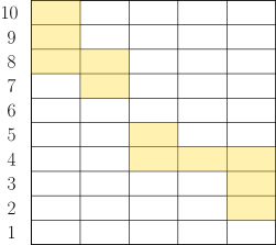
Figure 3: Representation of the down-right sequence of cells (highlighted) encoded by the admissible sequence $\big{(}(10,8),(8,7),(5,4),(4,4),(4,2)\big{)}$, with $K=5$ and $\beta=2$.

Say a sequence of indices $(\mathbf{a},\mathbf{b})=(a_{i},b_{i})_{1\leq i\leq K}$ is admissible if it satisfies $1\leq b_{i+1}\leq a_{i+1}\leq b_{i}\leq a_{i}\leq K\beta$ for all $i\in[K-1]$. Informally, it encodes a down-right sequence of cells where $a_{i}$, resp. $b_{i}$, is the highest, resp. lowest, cell in the $i$-th column. See Figure 3 for a representation. Fix such $(\mathbf{a},\mathbf{b})$ and write $\widetilde{\mathcal{P}}_{(\mathbf{a},\mathbf{b})}$ for the restriction of $\widetilde{\mathcal{P}}$ to the cells associated with $(\mathbf{a},\mathbf{b})$. For each $1\leq i\leq K$, write

$$R_{i}:=[(i-1)\Delta x,i\Delta x]\times[(b_{i}-1)\Delta y,a_{i}\Delta y]$$

for the $i$-th column of $(\mathbf{a},\mathbf{b})$, and set $h_{i}:=a_{i}-b_{i}+1$. Since $(\mathbf{a},\mathbf{b})$ encodes a down-right path, we can write

$$\mathrm{LDS}\big{(}\widetilde{\mathcal{P}}_{(\mathbf{a},\mathbf{b})}\big{)}\leq\sum_{i=1}^{K}\mathrm{LDS}(\widetilde{\mathcal{P}}\cap R_{i}).$$ (7)

Furthermore, at most one column $R_{i}$ can intersect the diagonal square cells $C_{i,i}$. When this happens, write $i_{0}$ for the corresponding index, and arbitrarily set $i_{0}:=1$ otherwise. Now notice that, by the Cauchy–Schwarz inequality:

$$\sum_{i=1}^{K}\sqrt{h_{i}\Delta x\Delta y}\leq\sqrt{K\sum_{i=1}^{K}h_{i}\Delta x\Delta y}\leq\sqrt{K\Delta x\Delta y(K+K\beta)}=\sqrt{1+\delta}$$

where the middle inequality is obtained by noticing that a down-right path has at most $K+K\beta$ cells. This yields

$$1+2\delta\geq\delta+\sqrt{1+\delta}\sum_{i=1}^{K}\sqrt{h_{i}\Delta x\Delta y}.$$ (8)

Using Equations 7 and 8, we deduce:

$$\mathbf{P}\left(\mathrm{LDS}\big{(}\widetilde{\mathcal{P}}_{(\mathbf{a},\mathbf{b})}\big{)}>2(1+2\delta)\sqrt{n}\right)\\ \leq\mathbf{P}\left(\exists i\neq i_{0},\;\mathrm{LDS}(\mathcal{P}\cap R_{i})>2\sqrt{1+\delta}\sqrt{nh_{i}\Delta x\Delta y}\right)+\mathbf{P}\left(\mathrm{LDS}\big{(}\widetilde{\mathcal{P}}\cap R_{i_{0}}\big{)}>2\delta\sqrt{n}\right).$$ (9)

We can decompose the family $\widetilde{\mathcal{P}}\cap R_{i_{0}}=(\mathcal{P}\cap A)\sqcup(\mathcal{P}\cap B)$ into its points above and below $C_{i_{0},i_{0}}$. Since we have $\mathrm{Leb}(A)\leq\Delta x<\delta^{2}/16$, 3.2 yields:

$$\mathbf{P}\left(\left|\mathcal{P}\cap A\right|>\frac{\delta^{2}}{16}n\right)\leq\exp\left(-c_{\delta}n\right),$$

and likewise for $B$. 3.3 asserts that the sets $\mathcal{P}\cap A$ and $\mathcal{P}\cap B$ consist of i.i.d. uniform points, hence:

$$\mathbf{P}\left(\mathrm{LDS}\big{(}\widetilde{\mathcal{P}}\cap R_{i_{0}}\big{)}>2\delta\sqrt{n}\right)\leq\mathbf{P}\left(L_{\left|\mathcal{P}\cap A\right|}>\delta\sqrt{n}\right)+\mathbf{P}\left(L_{\left|\mathcal{P}\cap B\right|}>\delta\sqrt{n}\right)\leq 2\mathbf{P}\left(L_{\frac{\delta^{2}}{16}n}>\delta\sqrt{n}\right)+\exp(-c_{\delta}n).$$

Therefore, by [DZ99, Theorem 2]:

$$\mathbf{P}\left(\mathrm{LDS}\big{(}\widetilde{\mathcal{P}}\cap R_{i_{0}}\big{)}>2\delta\sqrt{n}\right)\leq\exp\left(-c_{\delta}\sqrt{n}\right).$$ (10)

The first term of (9) is handled in a similar way. If $i\neq i_{0}$, by 3.2:

$$\mathbf{P}\left(\Big{.}\left|\mathcal{P}\cap R_{i}\right|>(1+\tfrac{\delta}{2})nh_{i}\Delta x\Delta y\right)\leq\exp\left(-c_{\delta}n\right).$$

We can then use 3.3 and [DZ99, Theorem 2] as before:

$$\mathbf{P}\left(\exists i\neq i_{0},\;\mathrm{LDS}(\mathcal{P}\cap R_{i})>2\sqrt{1+\delta}\sqrt{nh_{i}\Delta x\Delta y}\right)\\ \leq K\exp\left(-c_{\delta}n\right)+K\max_{i\neq i_{0}}\mathbf{P}\left(L_{(1+\frac{\delta}{2})nh_{i}\Delta x\Delta y}>2\sqrt{1+\delta}\sqrt{nh_{i}\Delta x\Delta y}\right)\leq\exp\left(-c_{\delta}\sqrt{n}\right).$$ (11)

Finally, putting together Equations 9, 10 and 11:

$$\mathbf{P}\left(\mathrm{LDS}\big{(}\widetilde{\mathcal{P}}_{(\mathbf{a},\mathbf{b})}\big{)}>2(1+2\delta)\sqrt{n}\right)\leq\exp\left(-c_{\delta}\sqrt{n}\right).$$

Since any down-right path of points defines an admissible sequence and the number of admissible sequences is bounded by $(K\beta)^{2K}$, we deduce:

$$\mathbf{P}\left(\Big{.}\mathrm{LDS}(\check{\mathcal{P}})>2(1+2\delta)\sqrt{n}\right)\leq\exp\left(-c_{\delta}\sqrt{n}\right)$$

for some constant $c_{\delta}>0$ which depends only on $\delta$. Using (6), this concludes the proof of the upper tail bound.

Lower tail bound:

Define $C:=[0,1/2]\times[1/2,1]$ and $C^{*}:=[1/2,1]\times[0,1/2]$. Then:

$$\mathrm{LDS}(\mathcal{P})\geq\mathrm{LDS}(\mathcal{P}\cap C)+\mathrm{LDS}(\mathcal{P}\cap C^{*}).$$

We can apply 3.2 to obtain

$$\mathbf{P}\left(\Big{.}\left|\mathcal{P}\cap C\right|<(1-\delta/2)^{2}n/4\right)\leq\exp\left(-2c_{\delta}n\right)$$

for some $c_{\delta}>0$, therefore by 3.3 and [DZ99, Theorem 1]:

$$\mathbf{P}\left(\Big{.}\mathrm{LDS}(\mathcal{P}\cap C)<(1-\delta)\sqrt{n}\right)\leq\exp\left(-2c_{\delta}n\right)+\mathbf{P}\left(L_{(1-\delta/2)^{2}n/4}<2(1-\delta)\sqrt{n/4}\right)\leq\exp\left(-c_{\delta}n\right)$$

and likewise for $C^{*}$. Finally:

$$\mathbf{P}\left(\Big{.}\mathrm{LDS}(\tau_{n})<2(1\!-\!\delta)\sqrt{n}\right)\leq\mathbf{P}\left(\Big{.}\mathrm{LDS}(\mathcal{P}\cap C)<(1\!-\!\delta)\sqrt{n}\right)+\mathbf{P}\left(\Big{.}\mathrm{LDS}(\mathcal{P}\cap C^{*})<(1\!-\!\delta)\sqrt{n}\right)\leq\exp\left(-c_{\delta}n\right)$$

for some $c_{\delta}>0$, as desired.

Convergence in probability readily follows from these inequalities. To obtain $L^{q}$ convergence for all $q\geq 1$ we simply need to prove boundedness in $n$ of $\mathbb{E}\left[\left(\mathrm{LDS}(\tau_{n})/\sqrt{n}\right)^{q^{\prime}}\right]$ for any ${q^{\prime}}\geq 1$. This follows from

$$\mathbb{E}\left[\left(\mathrm{LDS}(\tau_{n})/\sqrt{n}\right)^{q^{\prime}}\right]\leq(2+\delta)^{q^{\prime}}+(n/\sqrt{n})^{q^{\prime}}\exp\left(-c_{\delta}\sqrt{n}\right)=\underset{n\to\infty}{\mathcal{O}}\left(1\right)$$

where $\delta>0$ is arbitrary. This concludes the proof of Theorem 2.1. ∎

Proof of 2.2.

We work conditionally given $t^{(n)}$. Then for each $n$, $\tau_{n}$ is a uniform $t^{(n)}$-cyclic permutation. Let $\mathcal{P}$ be a geometric construction of $\tau_{n}$ and $\check{\mathcal{P}}$ be its points outside the diagonal. Define $\check{t}^{(n)}$ as the cycle type $(0,t_{2}^{(n)},t_{3}^{(n)},\dots)$ of size $\check{n}:=n-t_{1}^{(n)}$. Then according to 1.1, $\check{\tau}_{n}:={\rm Perm}\left(\check{\mathcal{P}}\right)$ is a uniform $\check{t}^{(n)}$-cyclic permutation. Since fixed points contribute at most $1$ to $\mathrm{LDS}(\tau_{n})$, we can write:

$$\mathrm{LDS}(\check{\tau}_{n})\leq\mathrm{LDS}(\tau_{n})\leq 1+\mathrm{LDS}(\check{\tau}_{n}).$$

Thus by Theorem 2.1, for any $\delta>0$ there exists a universal constant $c_{\delta}>0$ such that for any $n$:

$$\mathbf{P}\left(\mathrm{LDS}(\tau_{n})>2(1+\delta)\sqrt{\check{n}}\right)\leq\mathbb{E}\left[\mathbf{P}\left(\left.\mathrm{LDS}(\check{\tau}_{n})>2(1+\delta)\sqrt{\check{n}}\quad\right|t^{(n)}\right)\right]\\ \leq\mathbb{E}\left[\exp\left(-c_{\delta}\sqrt{\check{n}}\right)\right],$$

and likewise for the lower tail bound. If $\check{n}\to\infty$ in probability then the right-hand side goes to $0$ as $n\to\infty$, and this proves convergence in probability. Convergence in $L^{q}$ follows as in the proof of Theorem 2.1, bounding $\mathrm{LDS}(\tau_{n})$ above by $n-t_{1}^{(n)}+1$ and using the fact that the previous tail inequalities hold a.s. conditionally given $t^{(n)}$. ∎

4.2 Increasing subsequences

Proof of 2.3.

Fix $\delta>0$. Let $\mathcal{P}$ be a geometric construction of $\tau_{n}$ as in 1.1.

Lower tail bound:

Set $K=\lceil 2/\delta\rceil$ and let $(C_{i,j})_{1\leq i,j\leq K}$ be a regular square grid defined by

$$C_{i,j}=[(i\!-\!1)/K,i/K]\times[(j\!-\!1)/K,j/K].$$

Then:

$$\mathrm{LIS}(\tau_{n})=\mathrm{LIS}(\mathcal{P})\geq\sum_{i=1}^{K-1}\mathrm{LIS}(\mathcal{P}\cap C_{i,i\!+\!1}).$$ (12)

Using 3.2, there exists $c_{\delta}>0$ such that:

$$\mathbf{P}\left(\Big{.}\left|\mathcal{P}\cap C_{i,i\!+\!1}\right|<(1-\delta/2)^{2}n/K^{2}\right)\leq\exp\left({-2c_{\delta}n}\right).$$

Then by [DZ99, Theorem 1] along with 3.3, denoting by $L_{m}$ the $\mathrm{LIS}$ of a uniform permutation of size $m$:

$$\mathbf{P}\left(\big{.}\mathrm{LIS}(\mathcal{P}\cap C_{i,i\!+\!1})<(1-\delta)\frac{2\sqrt{n}}{K-1}\right)\leq\mathbf{P}\left(L_{(1-\delta/2)^{2}n/K^{2}}<(1-\delta)\frac{2\sqrt{n}}{K-1}\right)+\exp\left(-2c_{\delta}n\right)\leq\exp\left({-c_{\delta}n}\right)$$

since $\frac{1-\delta/2}{K}>\frac{1-\delta}{K-1}$. Finally, using Equation 12:

$$\mathbf{P}\left(\Big{.}\mathrm{LIS}(\tau_{n})<(1-\delta)2\sqrt{n}\right)\leq(K-1)\max_{1\leq i\leq K-1}\mathbf{P}\left(\big{.}\mathrm{LIS}(\mathcal{P}\cap C_{i,i\!+\!1})<(1-\delta)\frac{2\sqrt{n}}{K-1}\right)\leq\exp\left({-c_{\delta}n}\right)$$

for some $c_{\delta}>0$.

Upper tail bound:

For this, simply use 3.1 and a rough union bound. Since

$$\mathrm{LIS}(\tau_{n})=\mathrm{LIS}(\mathcal{P})\leq\mathrm{LIS}(\mathcal{P}^{(1)})+\mathrm{LIS}(\mathcal{P}^{(2)})+\mathrm{LIS}(\mathcal{P}^{(3)}),$$

we can use [DZ99, Theorem 2] to deduce

$$\mathbf{P}\left(\mathrm{LIS}(\tau_{n})>(1+\delta)2\sqrt{3n}\right)\leq 3\mathbf{P}\left(L_{\lceil n/3\rceil+1}>(1+\delta)2\sqrt{n/3}\right)\leq\exp\left(-c_{\delta}\sqrt{n}\right).$$

for some $c_{\delta}>0$. This concludes the proof. ∎

Proof of 2.4.

The method is the same as in the proof of 2.2, using rather the bounds

$$\max\left(t_{1}^{(n)},\mathrm{LIS}(\check{\tau}_{n})\right)\leq\mathrm{LIS}(\tau_{n})\leq t_{1}^{(n)}+\mathrm{LIS}(\check{\tau}_{n})$$

and discussing whether $t_{1}^{(n)}\geq(1-\delta)2\sqrt{n}$ for the upper tail bound. ∎

5 Proofs of the results on Robinson–Schensted shapes

Our proof of Theorem 2.7 relies heavily on the substantial work of Sjöstrand [Sjö23]. Let us recall a few definitions from the latter.

Let $\Omega$ be an open subset of $\mathbb{R}^{2}$. If $u:\Omega\to\mathbb{R}$ is Lebesgue-measurable, we write $\lVert u\rVert_{1,\Omega}:=\int_{\Omega}\left|u\right|d\mathrm{Leb}$ for its $L^{1}$ norm. Say that $u$ is doubly increasing if $u(x,y)\leq u(x^{\prime},y^{\prime})$ whenever $(x,y)\leq(x^{\prime},y^{\prime})$. Denote by $\mathcal{U}(\Omega)$ the set of doubly increasing functions on $\Omega$, and by $\mathcal{U}_{h,r}(\Omega)$ its subset consisting of functions with values in $[h,h+r]$. For any $u\in\mathcal{U}(\Omega)$, let

$$D(u):=\left\{\Big{.}(x,y)\in\Omega\,:\,u(x,y)\in\mathbb{Z}\text{ and }u(x^{\prime},y^{\prime})<u(x,y)\text{ for any }(x^{\prime},y^{\prime})\in\Omega\setminus\{(x,y)\}\text{ s.t. }(x^{\prime},y^{\prime})\leq(x,y)\right\}.$$

Informally, $D(u)$ is the set of “south-west corners” in the integer level lines of $u$. If $u\in\mathcal{U}_{0,r}(\Omega)$ then $D(u)$ is an $\lfloor r\rfloor$-decreasing subset of $\Omega$ [Sjö23, Lemma 6.2]. Reciprocally, for any finite $k$-decreasing subset $P$ of $\Omega$, there exists a $\kappa_{P}\in\mathcal{U}_{0,k}(\Omega)$ such that $D(\kappa_{P})=P$ [Sjö23, Definition 3.7 and Lemma 6.2]. Therefore, if $\mathcal{P}$ is a finite subset of $\Omega$:

$$\mathrm{LDS}_{r\sqrt{n}}(\mathcal{P})=\max_{w\in\mathcal{U}_{0,r}(\Omega)}\left|D(w\sqrt{n})\cap\mathcal{P}\right|.$$ (13)

Sjöstrand also introduces in [Sjö23, Definition 3.8] a certain function $L:\mathbb{R}_{+}^{2}\rightarrow\mathbb{R}_{+}$, and then for any Lebesgue-integrable function $\rho:\Omega\to\mathbb{R}_{+}$ and $u\in\mathcal{U}(\Omega)$ he defines $F_{\rho}(u):=\lVert L(\rho,\partial_{x}u\,\partial_{y}u)\rVert_{1,\Omega}$. We shall only need this functional when $\rho$ is constant to $1$ on $\Omega$, and we rather write $F_{\Omega}$ in this case. $F_{\Omega}(u)$ can be interpreted as a “score” associated with $u$: it serves as a limit approximation of $\left|D(w\sqrt{n})\cap\mathcal{P}\right|/n$, when $\sigma_{n}$ is a homogeneous Poisson point process of intensity $n$ on $\Omega$ and $w$ is close to $\sigma_{n}$. This informal idea is justified by [Sjö23, Lemmas 8.2 and 6.3], used here to prove the lower and upper bounds of Theorem 2.7.

Thanks to Theorem 2.6 and [Sjö23, Theorem 10.2], it holds that

$$F_{\mathrm{LSKV}}(r)=\sup_{u\in\mathcal{U}_{0,r}\left((0,1)^{2}\right)}F_{(0,1)^{2}}(u).$$ (14)

Proof of Theorem 2.7.

Fix $r\geq 0$. Let $\mathcal{P}$ be a geometric construction of $\tau_{n}$. The reason we can apply the results of [Sjö23] is that $\mathcal{P}$ is locally, outside the diagonal, close to a homogeneous Poisson point process with intensity $n$. More precisely, let $I,J$ be essentially disjoint intervals of $[0,1]$ and write $\bigtriangleup$ for the symmetric difference of sets. Thanks to 3.2 and 3.3, one can construct a homogeneous Poisson point process with intensity $n$ on $I\times J$, say $\sigma_{n}$, such that ${\left|\sigma_{n}\bigtriangleup\mathcal{P}\right|}/{n}\to 0$ as $n\to\infty$ almost surely.

Fix a large integer $K$, set $\epsilon:=1/K^{2}$, and define bands

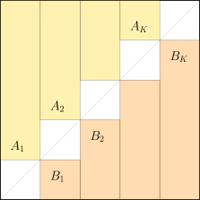
Figure 4: The bands defined in the proof of Theorem 2.7. On each $A_{i}$ and each $B_{i}$, $\mathcal{P}$ is almost distributed like a homogeneous Poisson point process.

$$A_{i}:=\left(\frac{i-1}{K+1},\frac{i}{K+1}\right)\times\left(\frac{i}{K+1},1\right)\quad\text{ and }\quad B_{i}:=\left(\frac{i}{K+1},\frac{i+1}{K+1}\right)\times\left(0,\frac{i}{K+1}\right)$$

for $i\in[K]$, see Figure 4. These bands each fit in the setting of 3.3, and they satisfy $\mathrm{Leb}(C)=\frac{1}{K+1}$ where $C:=(0,1)^{2}\setminus\left(\bigcup_{i}\bar{A}_{i}\cup\bar{B}_{i}\right)$. Moreover, using 3.2 and 3.3 as above, we can construct a point process $\sigma_{n}$ on $(0,1)^{2}$ such that:

1. for each $i\in[K]$, $\sigma_{n}\cap A_{i}$ and $\sigma_{n}\cap B_{i}$ are both distributed like homogeneous Poisson point processes with intensity $n$;

2. $\sigma_{n}$ coincides with $\mathcal{P}$ on $C$;

3. $\left|\sigma_{n}\bigtriangleup\mathcal{P}\right|/{n}\to 0$ as $n\to\infty$, almost surely.

From here, the arguments for the lower and upper bounds differ.

Upper bound:

For each $i\in[K]$, we can apply [Sjö23, Lemma 8.2] to $\sigma_{n}$ on $A_{i}$. Hence for any $u\in\mathcal{U}(A_{i})$, there exists $\delta_{u,A_{i}}>0$ such that:

$$\sup_{w\in\mathcal{U}(A_{i}),\,\lVert w-u\rVert_{1,A_{i}}<\delta_{u,A_{i}}}\left|D(w\sqrt{n})\cap\sigma_{n}\cap A_{i}\right|/n<F_{A_{i}}(u)+\epsilon$$

holds w.h.p. as $n\to\infty$. The same holds with $B_{i}$ instead of $A_{i}$. Moreover, a.s. for any $n$:

$$\sup_{w\in\mathcal{U}(C)}\left|D(w\sqrt{n})\cap\sigma_{n}\cap C\right|/n<\left|\sigma_{n}\cap C\right|/n=\left|\mathcal{P}\cap C\right|/n.$$

Since the property of being doubly increasing is stable by restriction, for any $u\in\mathcal{U}\left((0,1)^{2}\right)$ we can write

$$F_{(0,1)^{2}}(u)=F_{C}(u)+\sum_{i=1}^{K}(F_{A_{i}}(u)+F_{B_{i}}(u))\geq\sum_{i=1}^{K}(F_{A_{i}}(u)+F_{B_{i}}(u)).$$

By summing the previous inequalities we deduce that for any $u\in\mathcal{U}\left((0,1)^{2}\right)$, with $\delta_{u}:=\min_{1\leq i\leq K}\delta_{u,A_{i}}\wedge\delta_{u,B_{i}}$:

$$\sup_{w\in\mathcal{U}\left((0,1)^{2}\right),\,\lVert w-u\rVert_{1,(0,1)^{2}}<\delta_{u}}\left|D(w\sqrt{n})\cap\sigma_{n}\right|/n<F_{(0,1)^{2}}(u)+2K\epsilon+\left|\mathcal{P}\cap C\right|/n$$

w.h.p. as $n\to\infty$. Therefore:

$$\sup_{w\in\mathcal{U}\left((0,1)^{2}\right),\,\lVert w-u\rVert_{1,(0,1)^{2}}<\delta_{u}}\left|D(w\sqrt{n})\cap\mathcal{P}\right|/n<F_{(0,1)^{2}}(u)+2K\epsilon+\left|\mathcal{P}\cap C\right|/n+\left|\sigma_{n}\bigtriangleup\mathcal{P}\right|/n$$

w.h.p. as $n\to\infty$. Recall that $\epsilon=1/K^{2}$ and a.s. $\left|\sigma_{n}\bigtriangleup\mathcal{P}\right|/n\to 0$ as $n\to\infty$. Moreover 3.2 implies that a.s. $\left|\mathcal{P}\cap C\right|/n\to\mathrm{Leb}(C)=1/(K+1)$ as $n\to\infty$. Hence for any $u\in\mathcal{U}\left((0,1)^{2}\right)$:

$$\sup_{w\in\mathcal{U}\left((0,1)^{2}\right),\,\lVert w-u\rVert_{1,(0,1)^{2}}<\delta_{u}}\left|D(w\sqrt{n})\cap\mathcal{P}\right|/n<F_{(0,1)^{2}}(u)+4/K$$

w.h.p. as $n\to\infty$. According to [Sjö23, Proposition 9.2], $\mathcal{U}_{0,r}\left((0,1)^{2}\right)$ is compact for the $L^{1}$ metric. Thus its open cover

$$\mathcal{U}_{0,r}\left((0,1)^{2}\right)=\bigcup_{u\in\mathcal{U}_{0,r}\left((0,1)^{2}\right)}\left\{w\,:\,\lVert w-u\rVert_{1,(0,1)^{2}}<\delta_{u}\right\}$$

admits a finite subcover, and we can conclude that with high probability as $n\to\infty$:

$$\text{for any }w\in\mathcal{U}_{0,r}\left((0,1)^{2}\right),\quad\left|D(w\sqrt{n})\cap\mathcal{P}\right|/n<\sup_{u\in\mathcal{U}_{0,r}\left((0,1)^{2}\right)}F_{(0,1)^{2}}(u)+4/K.$$

Using Equations 14 and 13, this yields

$$\frac{1}{n}\mathrm{LDS}_{r\sqrt{n}}(\mathcal{P})<F_{\mathrm{LSKV}}(r)+4/K$$ (15)

w.h.p. as $n\to\infty$.

Lower bound:

The lower bound requires more work, and we need to delve deeper into the proofs of [Sjö23]. The reader is thus kindly invited to follow along with his own copy of [Sjö23]. Our proof hinges on the notation of [Sjö23, Definition 7.3], the results [Sjö23, Lemmas 4.9, 6.3, 7.7, 9.1], and the method behind [Sjö23, Lemma 10.1].

Recall (14) and fix $u\in\mathcal{U}_{0,r}\left((0,1)^{2}\right)$ such that

$$F_{(0,1)^{2}}(u)>F_{\mathrm{LSKV}}(r)-1/K.$$ (16)

Our goal is to construct a large enough $r\sqrt{n}$-decreasing subset of $\mathcal{P}$, i.e. by (13) to construct $w_{n}\in\mathcal{U}_{0,r}\left((0,1)^{2}\right)$ such that $\left|D(w_{n}\sqrt{n})\cap\mathcal{P}\right|/n\geq F_{(0,1)^{2}}(u)-\epsilon^{\prime}$ for some small $\epsilon^{\prime}$ and large enough $n$. Unfortunately we can not simply apply [Sjö23, Lemma 10.1] to each $A_{i}$ and $B_{i}$, as combining the resulting local, doubly increasing, functions into a single global, doubly increasing, function on $(0,1)^{2}$ would be difficult. Instead we rewrite the proof of this result in our framework: everything works the same, with the exception that we need to work on each $A_{i}$ and $B_{i}$ individually.

First apply [Sjö23, Lemma 7.7] to each domain $A_{i}\cup B_{i}$ with constant density $\rho=1$: since the density is constant, some items of this lemma become vacuous, and we only rewrite the relevant ones. Recall that we use the notation of [Sjö23, Definition 7.3]. For any $\iota\in(0,1/2)$ there exists a measurable subset $S_{\iota}^{i}\subseteq A_{i}\cup B_{i}$ on which $u$ is differentiable, and a finite collection $\mathfrak{P}_{\iota}^{i}$ of disjoint $(u,\iota)$-parallelograms, such that:

• $S_{\iota}^{i}\subseteq\bigcup_{P\in\mathfrak{P}_{\iota}^{i}}P$;

• $\partial_{x}u$ and $\partial_{y}u$ are bounded on $\bigcup_{0<\iota<1/2}S_{\iota}^{i}$;

• $\mathrm{Leb}(A_{i}\cup B_{i}\setminus S_{\iota}^{i})<\epsilon+o_{\iota}(1)$;

and for each $P\in\mathfrak{P}_{\iota}^{i}$:

• $P\subseteq A_{i}\cup B_{i}$, with center $(x_{P},y_{P})\in S_{\iota}^{i}$;

• if we denote by $u_{x}^{P},u_{y}^{P}$ the partial derivatives of $u$ at $(x_{P},y_{P})$, then for all $(x,y)\in P$:

  $$\left|u(x,y)-\left(u(x_{P},y_{P})+(x-x_{P})u_{x}^{P}+(y-y_{P})u_{y}^{P}\right)\right|\leq\iota^{5}\left(\left|x-x_{P}\right|+\left|y-y_{P}\right|\right);$$

• $\left|\frac{1}{\mathrm{Leb}(P)}F_{P}(u)-L(1,u_{x}^{P}u_{y}^{P})\right|<\iota$.

Then for each $\iota$, set $S_{\iota}:=\bigcup_{i\in[K]}S_{\iota}^{i}$ and $\mathfrak{P}_{\iota}:=\bigcup_{i\in[K]}\mathfrak{P}_{\iota}^{i}$. Note that, given our definition, any parallelogram contained in $A_{i}\cup B_{i}$ is either wholly contained in $A_{i}$, or wholly contained in $B_{i}$. Now let us follow the proof of [Sjö23, Lemma 10.1].

Fix $\iota\in(0,1/2)$. For each $P\in\mathfrak{P}_{\iota}$, let $P^{\prime}$ denote this parallelogram shrunk by a factor $1\!-\!2\iota$ in width and height. Denote by $\widetilde{\mathfrak{P}}_{\iota}$ the set of well-behaved parallelograms in $\mathfrak{P}_{\iota}$, i.e. for which we have $u_{x}^{P}\geq\iota^{3}$ and $u_{y}^{P}\geq\iota^{3}$. For each $P\in\mathfrak{P}_{\iota}$, let $\bar{u}_{P}\in\mathcal{U}(P)$ be defined by

$$\text{for all }(x,y)\in P,\quad\bar{u}_{P}(x,y):=u(x_{P},y_{P})+(x-x_{P})u_{x}^{P}+(y-y_{P})u_{y}^{P}$$

if $P\in\widetilde{\mathfrak{P}}_{\iota}$, and by $\bar{u}_{P}:=u$ on $P$ if $P\in\mathfrak{P}_{\iota}\setminus\widetilde{\mathfrak{P}}_{\iota}$. Let $r_{P}:=\mathrm{diam}\,\bar{u}_{P}(P^{\prime})$. Since $\sigma_{n}$ is distributed like a homogeneous Poisson point process with intensity $n$ on each $A_{i}$ and each $B_{i}$, we can apply [Sjö23, Lemma 6.3] to $\bar{u}_{P}$ and obtain the following analog of [Sjö23, Equation (18)]. For any $P\in\widetilde{\mathfrak{P}}_{\iota}$, w.h.p. as $n\to\infty$ there exists $w_{P}^{(n)}\in\mathcal{U}_{u(x_{P},y_{P})-\frac{r_{P}}{2},r_{P}}(P^{\prime})$ such that

$$\frac{1}{\mathrm{Leb}(P^{\prime})}\left|D\left(w_{P}^{(n)}\sqrt{n}\right)\cap\sigma_{n}\cap P^{\prime}\right|/n\geq L(1,u_{x}^{P}u_{y}^{P})-o_{\iota}(1)$$ (17)

where $o_{\iota}(1)\to 0$ as $\iota\to 0$, uniformly in $P$ and $n$. By [Sjö23, Lemma 4.9] and item (b), the function $L$ is uniformly continuous on the bounded set $\left\{\left(1,\partial_{x}u(x,y)\,\partial_{y}u(x,y)\big{.}\right)\,:\,(x,y)\in\bigcup_{\iota}S_{\iota}\right\}$ and satisfies $L(1,0)=0$. By definition, for any $P\in\mathfrak{P}_{\iota}\setminus\widetilde{\mathfrak{P}}_{\iota}$ we have $\min\left(u_{x}^{P},u_{y}^{P}\right)<\iota^{3}$. Therefore for any $P\in\mathfrak{P}_{\iota}\setminus\widetilde{\mathfrak{P}}_{\iota}$ and any $w_{P}^{(n)}\in\mathcal{U}(P^{\prime})$, Equation 17 still holds.

Under the event that $w_{P}^{(n)}$ exists for all $P\in\widetilde{\mathfrak{P}}_{\iota}$, define a function $w_{n}$ on $\bigcup_{P\in\widetilde{\mathfrak{P}}_{\iota}}P^{\prime}\,\cup\,\left((0,1)^{2}\setminus\bigcup_{P\in\widetilde{\mathfrak{P}}_{\iota}}P\right)$ as follows: for any $P\in\widetilde{\mathfrak{P}}_{\iota}$, $w_{n}$ equals $w_{P}^{(n)}$ on $P^{\prime}$, and $w_{n}$ equals $u$ on $(0,1)^{2}\setminus\bigcup_{P\in\widetilde{\mathfrak{P}}_{\iota}}P$. As in the proof of [Sjö23, Lemma 10.1], $w_{n}$ is doubly increasing on this domain (this mainly uses [Sjö23, Definition 7.3], the definition of $P^{\prime}$, and item (f)). Then by [Sjö23, Lemma 9.1], this function can be extended to $w_{n}\in\mathcal{U}_{0,r}\left((0,1)^{2}\right)$. Therefore, using (17), we can write w.h.p. as $n\to\infty$:

$$\left|D(w_{n}\sqrt{n})\cap\sigma_{n}\right|/n\geq\sum_{P\in\mathfrak{P}_{\iota}}\left|D(w_{n}\sqrt{n})\cap\sigma_{n}\cap P^{\prime}\right|/n\geq\sum_{P\in\mathfrak{P}_{\iota}}\mathrm{Leb}(P^{\prime})\left(L(1,u_{x}^{P}u_{y}^{P})-o_{\iota}(1)\right)$$ (18)

where $o_{\iota}(1)$ is independent of $P$ and $n$. By item (g):

$$\sum_{P\in\mathfrak{P}_{\iota}}\mathrm{Leb}(P^{\prime})L(1,u_{x}^{P}u_{y}^{P})\geq(1\!-\!2\iota)^{2}\sum_{P\in\mathfrak{P}_{\iota}}\mathrm{Leb}(P)L(1,u_{x}^{P}u_{y}^{P})\geq(1\!-\!2\iota)^{2}F_{\bigcup_{P\in\mathfrak{P}_{\iota}}\!\!P}(u)-o_{\iota}(1).$$ (19)

By [Sjö23, Lemma 4.9], $0\leq L(1,\partial_{x}u\,\partial_{y}u)\leq 1$, and by items (a) and (c):

$$\mathrm{Leb}\left(\big{.}\bigcup_{P\in\mathfrak{P}_{\iota}}P\right)\geq\mathrm{Leb}\left(\bigcup_{i\in[K]}A_{i}\cup B_{i}\right)-K\epsilon-o_{\iota}(1)=1-2/K-o_{\iota}(1).$$

This implies $F_{\bigcup_{P\in\mathfrak{P}_{\iota}}\!\!P}(u)\geq F_{(0,1)^{2}}(u)-2/K-o_{\iota}(1)$. Along with (18) and (19), this yields:

$$\left|D(w_{n}\sqrt{n})\cap\sigma_{n}\right|/n\geq F_{(0,1)^{2}}(u)-2/K-o_{\iota}(1)$$

w.h.p. as $n\to\infty$, where $o_{\iota}(1)$ is uniform in $n$. Take $\iota$ such that this $o_{\iota}(1)$ is less that $1/K$. Then use Equations 13 and 16 and the property $\left|\sigma_{n}\bigtriangleup\mathcal{P}\right|/n\to 0$ to deduce

$$\frac{1}{n}\mathrm{LDS}_{r\sqrt{n}}(\mathcal{P})\geq F_{\mathrm{LSKV}}(r)-5/K$$ (20)

w.h.p. as $n\to\infty$.

Finally, we conclude the proof of Theorem 2.7 with Equations 15 and 20, as they hold for any $K$. ∎

Remark 7.

With the same arguments as in the proof of [Sjö23, Lemma 10.1], we could refine our proof of Theorem 2.7 to show that the longest decreasing subsequences of $\mathcal{P}$ are located on the same limit curves as in the uniform case (see [Sjö23, Theorem 10.2 (a)] for a precise statement).

Proof of 2.8.

Let $\mathcal{P}$ be a geometric construction of $\tau_{n}$. Since each decreasing subsequence of $\tau_{n}$ contains at most one fixed point, we can write:

$$\mathrm{LDS}_{k}(\check{\tau}_{n})\leq\mathrm{LDS}_{k}(\tau_{n})\leq\mathrm{LDS}_{k}(\check{\tau}_{n})+k$$

for any $k\geq 0$. Hence:

$$\mathbf{P}\left(\left|\frac{1}{\check{n}}\mathrm{LDS}_{r\sqrt{\check{n}}}(\tau_{n})-F_{\mathrm{LSKV}}(r)\right|>\epsilon\right)\leq\mathbf{P}\left(\left|\frac{1}{\check{n}}\mathrm{LDS}_{r\sqrt{\check{n}}}(\check{\tau}_{n})-F_{\mathrm{LSKV}}(r)\right|>\epsilon_{n}\right)$$

where $\epsilon_{n}:=\epsilon-\frac{r\sqrt{\check{n}}}{\check{n}}\underset{n\to\infty}{\longrightarrow}\epsilon$ in probability. Then by Theorem 2.7 and dominated convergence theorem:

$$\mathbf{P}\left(\left|\frac{1}{\check{n}}\mathrm{LDS}_{r\sqrt{\check{n}}}(\check{\tau}_{n})-F_{\mathrm{LSKV}}(r)\right|>\epsilon_{n}\right)\\ =\mathbb{E}\left[\mathbf{P}\left(\left|\frac{1}{\check{n}}\mathrm{LDS}_{r\sqrt{\check{n}}}(\check{\tau}_{n})-F_{\mathrm{LSKV}}(r)\right|>\epsilon_{n}\quad\Bigg{|}t^{(n)}\right)\right]\underset{n\to\infty}{\longrightarrow}0,$$

which concludes the proof. ∎

6 Proofs of the results on records

6.1 High records

Lemma 6.1.

For each $n$, let $t^{(n)}$ be a cycle type of size $n$ such that $t_{1}^{(n)}=0$, and $\mathcal{P}$ be a geometric construction. Set $C:=[0,1/2]\times[1/2,1]$. Define $Z_{\text{left}}=\left(U_{\text{left}},V_{\text{left}}\right)$ as the leftmost point in $\mathcal{P}$, $Z_{\text{left}}^{C}=\left(U_{\text{left}}^{C},V_{\text{left}}^{C}\right)$ as the leftmost point of $\mathcal{P}\cap C$, and let $Z_{\text{up}}$, $Z_{\text{up}}^{C}$ be the upmost analogues. Those points are well defined w.h.p. as $n\to\infty$ and:

$$\left(\big{.}nU_{\text{left}},n\left(1-V_{\text{up}}\right)\right)\underset{n\to\infty}{\longrightarrow}\left(E,E^{\prime}\right)\quad;\quad nU_{\text{left}}^{C}\underset{n\to\infty}{\longrightarrow}2E\quad;\quad n\left(1-V_{\text{up}}^{C}\right)\underset{n\to\infty}{\longrightarrow}2E$$

in distribution, where $E,E^{\prime}$ are independent ${\rm Exp}\left(1\right)$ variables. Furthermore, w.h.p. as $n\to\infty$ the inequalities $U_{\text{left}}\leq U_{\text{left}}^{C}\leq V_{\text{left}}$ hold.

Proof.

Recall from the geometric construction that the lists of x- and y-coordinates of points in $\mathcal{P}$ are both equal to the same family $\{U_{i}\}_{i\in\mathcal{V}_{t}}$ of i.i.d. ${\rm Unif}\left([0,1]\right)$ variables. Thus $U_{\text{left}}=:U_{(1)}$ is their minimum and $V_{\text{up}}=:U_{(n)}$ is their maximum. For any $s,t\geq 0$ we have:

$$\mathbf{P}\left(nU_{(1)}\geq s\;,\;n\left(1-U_{(n)}\right)\geq t\right)=\mathbf{P}\left(\big{.}\forall i,\;U_{i}\in[s/n,1-t/n]\right)=(1-(s+t)/n)^{n}\underset{n\to\infty}{\longrightarrow}e^{-s}e^{-t}.$$

This proves the first convergence in distribution. For the second one, use 3.3 and write, conditionally given $\left|\mathcal{P}\cap C\right|$:

$$\mathbf{P}\left(nU_{\text{left}}^{C}\geq s\right)=\left(1-\frac{s/(2n)}{1/4}\right)^{\left|\mathcal{P}\cap C\right|}=(1-2s/n)^{\left|\mathcal{P}\cap C\right|}.$$

According to 3.2, $\left|\mathcal{P}\cap C\right|$ is concentrated around $n/4$. This readily implies $\mathbf{P}\left(nU_{\text{left}}^{C}\geq s\right)\to e^{-s/2}$ as $n\to\infty$, and proves the second convergence in distribution. The third one follows similarly.

For the last claim, it suffices to note that $U_{\text{left}}$ and $U_{\text{left}}^{C}$ are both $o_{\mathbf{P}}(1)$ whereas $V_{\text{left}}$ has distribution ${\rm Unif}\left([0,1]\right)$, and $U_{\text{left}}\leq U_{\text{left}}^{C}$ by definition. ∎

Proof of Theorem 2.10.

Let $\mathcal{P}$ be a geometric construction of $\tau_{n}$. Decompose it into its points outside the diagonal $\check{\mathcal{P}}$ and its points on the diagonal $\mathcal{P}_{\Delta}$. We shall use the notation of 6.1, applied to the set $\check{\mathcal{P}}$ of size $\check{n}:=n-t_{1}^{(n)}$. According to this lemma, w.h.p. the point $Z_{\text{left}}$ is above the diagonal $\Delta$ and the rectangle $[U_{\text{left}},U_{\text{left}}^{C}]\times[V_{\text{left}},V_{\text{left}}^{C}]$ does not intersect $\Delta$. Likewise, w.h.p. the point $Z_{\text{up}}$ is above the diagonal and the rectangle $[U_{\text{up}}^{C},U_{\text{up}}]\times[V_{\text{up}}^{C},V_{\text{up}}]$ does not intersect $\Delta$. Under those events, the records of $\mathcal{P}$ are all contained in

$$\left(\Delta\cap[0,U_{\text{left}}]^{2}\right)\quad\bigcup\quad[U_{\text{left}},U_{\text{left}}^{C}]\times[V_{\text{left}},V_{\text{left}}^{C}]\quad\bigcup\quad C\quad\bigcup\quad[U_{\text{up}}^{C},U_{\text{up}}]\times[V_{\text{up}}^{C},V_{\text{up}}]\quad\bigcup\quad\left(\Delta\cap[V_{\text{up}},1]^{2}\right).$$

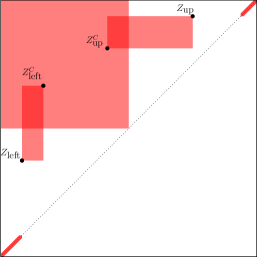
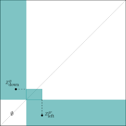
Figure 5: The zones in which we can find records (high ones on the left and low ones on the right).

This zone is shown on the left-hand side of Figure 5. Note that the rectangles $[U_{\text{left}},U_{\text{left}}^{C}]\times[V_{\text{left}},V_{\text{left}}^{C}]$ and $[U_{\text{up}}^{C},U_{\text{up}}]\times[V_{\text{up}}^{C},V_{\text{up}}]$ may be flat, i.e. the identities $U_{\text{left}}=U_{\text{left}}^{C}$ and $V_{\text{up}}^{C}=V_{\text{up}}$ may occur with non-negligible probability.

Invertly, all points of $\mathcal{P}_{\Delta}$ in $[0,U_{\text{left}}]^{2}\cup[V_{\text{up}},1]^{2}$, as well as the ones which are high records in $\mathcal{P}\cap C$, are high records in $\mathcal{P}$. From the previous two observations we deduce the following inequality w.h.p. as $n\to\infty$:

$$\left|\mathrm{rec}^{\uparrow}\left(\mathcal{P}\right)-\left(\Big{.}\mathrm{rec}^{\uparrow}\left(\check{\mathcal{P}}\cap C\right)+S_{n}\right)\right|\\ \leq\left|\check{\mathcal{P}}\cap\left([U_{\text{left}},U_{\text{left}}^{C}]\times[V_{\text{left}},V_{\text{left}}^{C}]\right)\right|+\left|\check{\mathcal{P}}\cap\left([U_{\text{up}}^{C},U_{\text{up}}]\times[V_{\text{up}}^{C},V_{\text{up}}]\right)\right|$$

where $S_{n}:=\left|\mathcal{P}_{\Delta}\cap[0,U_{\text{left}}]^{2}\right|+\left|\mathcal{P}_{\Delta}\cap[V_{\text{up}},1]^{2}\right|$. According to 6.1, $U_{\text{left}}^{C}$ is a $\mathcal{O}_{\mathbf{P}}\left(1/\check{n}\right)$. For any $M>0$, we may apply 3.2 to the rectangle $[0,M/\check{n}]\times[0,1]$ to obtain $\left|\check{\mathcal{P}}\cap\left([0,M/\check{n}]\times[0,1]\right)\right|\leq 2M$ w.h.p. as $n\to\infty$. Since $U_{\text{left}}^{C}\leq M/\check{n}$ with probability tending to $1$ as $M\to\infty$, uniformly in $n$, this implies that the variable $\left|\check{\mathcal{P}}\cap\left([U_{\text{left}},U_{\text{left}}^{C}]\times[V_{\text{left}},V_{\text{left}}^{C}]\right)\right|$ is a $\mathcal{O}_{\mathbf{P}}(1)$. With the same reasoning applied to $1-V_{\text{up}}^{C}$ and the corresponding rectangle, we deduce:

$$\left|\mathrm{rec}^{\uparrow}\left(\mathcal{P}\right)-\left(\Big{.}\mathrm{rec}^{\uparrow}\left(\check{\mathcal{P}}\cap C\right)+S_{n}\right)\right|=\mathcal{O}_{\mathbf{P}}(1).$$ (21)

Now it remains to analyse both terms in the sum. According to 3.3 and 3.2, $\check{\mathcal{P}}\cap C$ is a family of i.i.d. uniform points in $C$, with size $\check{n}/{4}+o_{\mathbf{P}}\left(\check{n}\right)$. We can thus apply Theorem 2.9 to deduce

$$\frac{\mathrm{rec}^{\uparrow}\left(\check{\mathcal{P}}\cap C\right)-\log\check{n}}{\sqrt{\log\check{n}}}\underset{n\to\infty}{\longrightarrow}{\cal N}\left(0,1\right)$$ (22)

in distribution. Let us turn to the fixed points. $\check{\mathcal{P}}$ and $\mathcal{P}_{\Delta}$ are independent, so $(U_{\text{left}},V_{\text{up}})$ and $\mathcal{P}_{\Delta}$ are as well. Therefore, conditionally given $(U_{\text{left}},V_{\text{up}})$, $S_{n}$ follows a ${\rm Binom}\left(t_{1}^{(n)},U_{\text{left}}\!+\!1\!-\!V_{\text{up}}\right)$ law. Recall from 6.1 that

$$\check{n}\left(U_{\text{left}}+1-V_{\text{up}}\right)\underset{n\to\infty}{\longrightarrow}\mathrm{Gamma}\left(2,1\right):={\rm Exp}\left(1\right)*{\rm Exp}\left(1\right)$$

in distribution. If ${t_{1}^{(n)}}/{\check{n}}=\mathcal{O}(1)$ as $n\to\infty$ then $S_{n}=\mathcal{O}_{\mathbf{P}}(1)$ (use e.g. the Bienaymé–-Chebyshev inequality), whereas if ${t_{1}^{(n)}}/{\check{n}}\to\infty$ as $n\to\infty$ then

$$\frac{\check{n}}{t_{1}^{(n)}}S_{n}\underset{n\to\infty}{\longrightarrow}\mathrm{Gamma}\left(2,1\right)$$ (23)

in distribution. Now we can use Equations 21, 22 and 23 to identify three regimes in the asymptotics of $\mathrm{rec}^{\uparrow}\left(\mathcal{P}\right)$.

“Mostly uniform” regime:

Assume $\frac{\check{n}}{n/\sqrt{\log n}}\to\infty$. Then $\log n\sim\log\check{n}$ as $n\to\infty$, and since $t_{1}^{(n)}\leq n$, we have $\frac{t_{1}^{(n)}}{\check{n}\sqrt{\log\check{n}}}\to 0$. Consequently the fluctuations of $\mathrm{rec}^{\uparrow}\left(\check{\mathcal{P}}\cap C\right)$ dominate, and

$$\frac{\mathrm{rec}^{\uparrow}\left(\mathcal{P}\right)-\log\check{n}}{\sqrt{\log\check{n}}}\underset{n\to\infty}{\longrightarrow}{\cal N}\left(0,1\right).$$

“Mostly fixed points” regime:

Assume $\frac{\check{n}}{n/\sqrt{\log n}}\to 0$ as $n\to\infty$. Since $\log\check{n}\leq\log n$ and $t_{1}^{(n)}=n-\check{n}$, we have $\frac{t_{1}^{(n)}}{\check{n}\sqrt{\log\check{n}}}\to\infty$. Consequently the fluctuations of $S_{n}$ dominate, and

$$\frac{\check{n}}{t_{1}^{(n)}}\left(\mathrm{rec}^{\uparrow}\left(\mathcal{P}\right)-\log\check{n}\right)\underset{n\to\infty}{\longrightarrow}\mathrm{Gamma}\left(2,1\right).$$

“Intermediate” regime:

Assume $\frac{\check{n}}{n/\sqrt{\log n}}\to\alpha\in(0,\infty)$. Then $\log\check{n}\sim\log n$ as $n\to\infty$, and since $t_{1}^{(n)}=n-\check{n}$, we deduce $\frac{t_{1}^{(n)}}{\check{n}\sqrt{\log\left(\check{n}\right)}}\to 1/\alpha$. Thus we need to understand the interplay between the limit laws of Equations 22 and 23. To do this, notice that conditionally given $\left(U_{\text{left}},V_{\text{up}}\right)$, the variables $S_{n}$ and $\check{\mathcal{P}}\cap C$ are independent. Recall that under this conditioning, $S_{n}$ follows a ${\rm Binom}\left(t_{1}^{(n)},U_{\text{left}}\!+\!1\!-\!V_{\text{up}}\right)$ law. According to 3.4, the conditional law of ${\rm Perm}\left(\check{\mathcal{P}}\cap C\right)$ given $\left(U_{\text{left}},V_{\text{up}}\right)=\left(U_{(1)},U_{(n)}\right)$ and $\left|\check{\mathcal{P}}\cap C\right|$ is uniform. From this property we deduce independence of the limit laws in Equations 23 and 22, whence:

$$\frac{\mathrm{rec}^{\uparrow}\left(\mathcal{P}\right)-\log\check{n}}{\frac{t_{1}^{(n)}}{\check{n}}+\sqrt{\log\check{n}}}=\frac{\mathrm{rec}^{\uparrow}\left(\check{\mathcal{P}}\cap C\right)-\log\check{n}}{(1+1/\alpha+o(1))\sqrt{\log\check{n}}}+\frac{S_{n}}{(1+\alpha+o(1))\frac{t_{1}^{(n)}}{\check{n}}}+o_{\mathbf{P}}(1)\\ \underset{n\to\infty}{\longrightarrow}\frac{\alpha}{\alpha+1}{\cal N}\left(0,1\right)*\frac{1}{1+\alpha}\mathrm{Gamma}\left(2,1\right)$$

in distribution, as announced. ∎

6.2 Low records

Lemma 6.2.

For each $n$, let $t^{(n)}$ be a cycle type of size $n$ such that $t_{1}^{(n)}=0$, and $\mathcal{P}$ be a geometric construction. Fix $\epsilon>0$ and define $B_{n}:=\left[0,\epsilon/\sqrt{n}\right]\times\left[\epsilon/\sqrt{n},1\right]$ and $B_{n}^{*}:=\left[\epsilon/\sqrt{n},1\right]\times\left[0,\epsilon/\sqrt{n}\right]$. Then

$$\frac{\left|\mathcal{P}\cap B_{n}\right|}{\epsilon\sqrt{n}}\underset{n\to\infty}{\longrightarrow}1\quad;\quad\frac{\left|\mathcal{P}\cap B_{n}^{*}\right|}{\epsilon\sqrt{n}}\underset{n\to\infty}{\longrightarrow}1$$

in probability. In particular w.h.p. we can define $Z_{\text{down}}^{B}=\left(U_{\text{down}}^{B},V_{\text{down}}^{B}\right)$ as the downmost point in $\mathcal{P}\cap B_{n}$ and $Z_{\text{left}}^{B^{*}}=\left(U_{\text{left}}^{B^{*}},V_{\text{left}}^{B^{*}}\right)$ as the leftmost point in $\mathcal{P}\cap B_{n}^{*}$, and they satisfy:

$${\epsilon\sqrt{n}}V_{\text{down}}^{B}-\epsilon^{2}\underset{n\to\infty}{\longrightarrow}{\rm Exp}\left(1\right)\quad;\quad{\epsilon\sqrt{n}}U_{\text{left}}^{B^{*}}-\epsilon^{2}\underset{n\to\infty}{\longrightarrow}{\rm Exp}\left(1\right)$$

in distribution.

Proof.

By 3.2, $\left|\mathcal{P}\cap B_{n}\right|$ is distributed like a sum of three ${\rm Binom}\left(\lfloor n/3\rfloor\pm 1,\left(1-\epsilon/\sqrt{n}\right)\big{.}\epsilon/\sqrt{n}\right)$, and likewise for $B_{n}^{*}$. The first claim readily follows from standard concentration inequalities. Then w.h.p. as $n\to\infty$, the sets $\mathcal{P}\cap B_{n}$ and $\mathcal{P}\cap B_{n}^{*}$ are non-empty and $Z_{\text{down}}^{B}$, $Z_{\text{left}}^{B^{*}}$ are well defined. According to 3.3, conditionally given $\left|\mathcal{P}\cap B_{n}\right|$, the set $\mathcal{P}\cap B_{n}$ consists of i.i.d. uniform points in $B_{n}$. We can thus write, for any $s>0$ and large enough $n$, conditionally given $\left|\mathcal{P}\cap B_{n}\right|$:

$$\mathbf{P}\left(\epsilon\sqrt{n}V_{\text{down}}^{B}>s+\epsilon^{2}\right)=\mathbf{P}\left(V_{\text{down}}^{B}>\frac{s}{\epsilon\sqrt{n}}+\epsilon/\sqrt{n}\right)=\left(1-\frac{1}{1-\epsilon/\sqrt{n}}\frac{s}{\epsilon\sqrt{n}}\right)^{\left|\mathcal{P}\cap B_{n}\right|}.$$

Hence $\mathbf{P}\left(\epsilon\sqrt{n}V_{\text{down}}^{B}>s+\epsilon^{2}\right)\to e^{-s}$ as $n\to\infty$. The same holds for $U_{\text{left}}^{B^{*}}$, and this concludes the proof. ∎

Proof of Theorem 2.11.

For each $n$, let $t^{(n)}$ be a cycle type of size $n$ and $\mathcal{P}$ be a geometric construction of $t^{(n)}$. Fix $\epsilon>0$.

Case 1:

Suppose $t_{1}^{(n)}=\mathcal{O}\left(\sqrt{n}\right)$.

Define $C_{n}:=\left[0,\epsilon/\sqrt{\check{n}}\right]^{2}$. Then $\left|\check{\mathcal{P}}\cap C_{n}\right|$ is distributed like a sum of three ${\rm Binom}\left(\lfloor\check{n}/3\rfloor\pm 1,\epsilon^{2}/\check{n}\right)$ variables by 3.2, and $\left|\mathcal{P}_{\Delta}\cap C_{n}\right|$ follows a ${\rm Binom}\left(t_{1}^{(n)},\epsilon/\sqrt{\check{n}}\right)$ law. Therefore there exists $\delta(\epsilon)=\underset{\epsilon\to 0}{o}\left(1\right)$, independent of $n$, such that:

$$\limsup_{n\to\infty}\mathbf{P}\left(\mathcal{P}\cap C_{n}\neq\emptyset\right)\leq\delta(\epsilon).$$ (24)

Define $B_{n}:=\left[0,\epsilon/\sqrt{\check{n}}\right]\times\left[\epsilon/\sqrt{\check{n}},1\right]$ and $B_{n}^{*}:=\left[\epsilon/\sqrt{\check{n}},1\right]\times\left[0,\epsilon/\sqrt{\check{n}}\right]$. According to 6.2 we can define w.h.p. $Z_{\text{down}}^{B}=\left(U_{\text{down}}^{B},V_{\text{down}}^{B}\right)$ as the downmost point in $\check{\mathcal{P}}\cap B_{n}$ and $Z_{\text{left}}^{B^{*}}=\left(U_{\text{left}}^{B^{*}},V_{\text{left}}^{B^{*}}\right)$ as the leftmost point in $\check{\mathcal{P}}\cap B_{n}^{*}$. See the right-hand side of Figure 5 for a representation.

Define the event $E_{n}:=\{\mathcal{P}\cap C_{n}=\emptyset\}\cap\left\{\check{\mathcal{P}}\cap B_{n}\neq\emptyset\right\}\cap\left\{\check{\mathcal{P}}\cap B_{n}^{*}\neq\emptyset\right\}$. Under this event, all points which are low records in $\check{\mathcal{P}}\cap B_{n}$ or in $\check{\mathcal{P}}\cap B_{n}^{*}$ are also low records in $\mathcal{P}$. Reciprocally, all low records of $\mathcal{P}$ lie in $B_{n}$, in $B_{n}^{*}$, or in $\left[\epsilon/\sqrt{\check{n}},U_{\text{left}}^{B^{*}}\right]\times\left[\epsilon/\sqrt{\check{n}},V_{\text{down}}^{B}\right]$. Hence under $E_{n}$:

$$\left|\Big{.}\mathrm{rec}^{\downarrow}\left(\mathcal{P}\right)-\mathrm{rec}^{\downarrow}\left(\check{\mathcal{P}}\cap B_{n}\right)-\mathrm{rec}^{\downarrow}\left(\check{\mathcal{P}}\cap B_{n}^{*}\right)\right|\leq\left|\mathcal{P}\cap\left(\left[\epsilon/\sqrt{\check{n}},U_{\text{left}}^{B^{*}}\right]\times\left[\epsilon/\sqrt{\check{n}},V_{\text{down}}^{B}\right]\right)\right|.$$ (25)

Using 6.2 and the fact that $t_{1}^{(n)}=\mathcal{O}\left(\sqrt{n}\right)$ we obtain:

$$\left|\mathcal{P}\cap\left(\left[\epsilon/\sqrt{\check{n}},U_{\text{left}}^{B^{*}}\right]\times\left[\epsilon/\sqrt{\check{n}},V_{\text{down}}^{B}\right]\right)\right|=\mathcal{O}_{\mathbf{P}}(1)$$

as $n\to\infty$, for fixed $\epsilon>0$. Thus it suffices to study the records in $B_{n}$ and $B_{n}^{*}$. We can apply 3.3, 6.2 and Theorem 2.9 to obtain

$$\frac{\mathrm{rec}^{\downarrow}\left(\check{\mathcal{P}}\cap B_{n}\right)}{\frac{1}{2}\log\left(n\right)}\underset{n\to\infty}{\longrightarrow}1$$

in probability, and likewise for $B_{n}^{*}$. Using Equations 25 and 24 we deduce that for any $\eta>0$:

$$\limsup_{n\to\infty}\mathbf{P}\left(\left|\frac{\mathrm{rec}^{\downarrow}\left(\mathcal{P}\right)}{\frac{1}{2}\log\left(n\right)}-2\right|>\eta\right)\leq\delta(\epsilon).$$

Since this holds for any $\epsilon>0$, the desired convergence in probability follows.

Case 2:

Suppose $\sqrt{n}=o\left(t_{1}^{(n)}\right)$.

Let $Z_{\Delta}=(U_{\Delta},U_{\Delta})$ be the leftmost point of $\mathcal{P}_{\Delta}$. Then it is standard that

$$t_{1}^{(n)}U_{\Delta}\underset{n\to\infty}{\longrightarrow}{\rm Exp}\left(1\right)$$ (26)

in distribution. By 3.2 and since ${\check{n}}/{(t_{1}^{(n)})^{2}}\to 0$, w.h.p. it holds that $\check{\mathcal{P}}\cap[0,U_{\Delta}]^{2}=\emptyset$. Define two bands $B_{\Delta}:=[0,U_{\Delta}]\times[U_{\Delta},1]$ and $B_{\Delta}^{*}:=[U_{\Delta},1]\times[0,U_{\Delta}]$. Then under the event $\left\{\check{\mathcal{P}}\cap[0,U_{\Delta}]^{2}=\emptyset\right\}$ we may write:

$$\mathrm{rec}^{\downarrow}\left(\mathcal{P}\right)=1+\mathrm{rec}^{\downarrow}\left(\check{\mathcal{P}}\cap B_{\Delta}\right)+\mathrm{rec}^{\downarrow}\left(\check{\mathcal{P}}\cap B_{\Delta}^{*}\right).$$ (27)

Using 3.2 and 3.3 conditionally given $U_{\Delta}$, $\check{\mathcal{P}}\cap B_{\Delta}$ is a family of i.i.d. uniform points in $B_{\Delta}$ whose size is distributed like a sum of three ${\rm Binom}\left(\lfloor\check{n}/3\rfloor\pm 1,U_{\Delta}(1-U_{\Delta})\right)$ variables. The same holds for $B_{\Delta}^{*}$.

• If $n=\mathcal{O}\left(t_{1}^{(n)}\right)$ then, by Equation 26, $\left|\mathcal{P}\cap B_{\Delta}\right|$ and $\left|\mathcal{P}\cap B_{\Delta}^{*}\right|$ are both $\mathcal{O}_{\mathbf{P}}(1)$ as $n\to\infty$. Thus by Equation 27, $\mathrm{rec}^{\downarrow}\left(\mathcal{P}\right)$ is also a $\mathcal{O}_{\mathbf{P}}(1)$.

• If $t_{1}^{(n)}=o(n)$ then, by Equation 26, $\frac{t_{1}^{(n)}}{n}\left|\mathcal{P}\cap B_{\Delta}\right|\underset{n\to\infty}{\longrightarrow}{\rm Exp}\left(1\right)$ in distribution. Therefore:

  $$\frac{\log\left|\mathcal{P}\cap B_{\Delta}\right|}{\log\left(n/t_{1}^{(n)}\right)}\underset{n\to\infty}{\longrightarrow}1$$

  in probability. In particular $\left|\mathcal{P}\cap B_{\Delta}\right|\to\infty$ in probability and we can apply Theorem 2.9 to deduce:

  $$\frac{\mathrm{rec}^{\downarrow}\left(\mathcal{P}\cap B_{\Delta}\right)}{\log\left|\mathcal{P}\cap B_{\Delta}\right|}\underset{n\to\infty}{\longrightarrow}1$$

  in probability. The same holds for $B_{\Delta}^{*}$, and the previous two equations along with Equation 27 yield:

  $$\frac{\mathrm{rec}^{\downarrow}\left(\mathcal{P}\right)}{\log\left(n/t_{1}^{(n)}\right)}\underset{n\to\infty}{\longrightarrow}2$$

  as desired.

This concludes the proof of Theorem 2.11. ∎

Proof of 2.12.

We use the same notation as in the proof of Theorem 2.11. Recall that under $E_{n}$:

$$\left|\mathrm{rec}^{\downarrow}\left(\mathcal{P}\right)-\mathrm{rec}^{\downarrow}\left(\check{\mathcal{P}}\cap B_{n}\right)-\mathrm{rec}^{\downarrow}\left(\check{\mathcal{P}}\cap B_{n}^{*}\right)\right|\leq\mathcal{O}_{\mathbf{P}}(1)$$ (28)

where by 3.3, 6.2 and Theorem 2.9:

$$\frac{\mathrm{rec}^{\downarrow}\left(\check{\mathcal{P}}\cap B_{n}\right)-\frac{1}{2}\log n}{\sqrt{\frac{1}{2}\log n}}\underset{n\to\infty}{\longrightarrow}{\cal N}\left(0,1\right)$$ (29)

in distribution, and likewise for $B_{n}^{*}$. It remains to understand how $\mathrm{rec}^{\downarrow}\left(\mathcal{P}\cap B_{n}\right)$ and $\mathrm{rec}^{\downarrow}\left(\mathcal{P}\cap B_{n}^{*}\right)$ are correlated.

Products of $2$-cycles:

Suppose that $t_{1}^{(n)}+2t_{2}^{(n)}=n$, i.e. that $\tau_{n}$ is a random involution with $t_{1}^{(n)}$ fixed points. Then the sets $\check{\mathcal{P}}\cap B_{n}$ and $\check{\mathcal{P}}\cap B_{n}^{*}$ are a.s. symmetric with respect to the diagonal. Therefore ${\rm Perm}\left(\check{\mathcal{P}}\cap B_{n}\right)$ and ${\rm Perm}\left(\check{\mathcal{P}}\cap B_{n}^{*}\right)$ are a.s. inverse of each other, and $\mathrm{rec}^{\downarrow}\left({\rm Perm}\left(\check{\mathcal{P}}\cap B_{n}\right)\right)=\mathrm{rec}^{\downarrow}\left({\rm Perm}\left(\check{\mathcal{P}}\cap B_{n}^{*}\right)\right)$ almost surely. Using Equations 24, 28 and 29 this yields:

$$\frac{\mathrm{rec}^{\downarrow}\left(\mathcal{P}\right)-\log n}{\sqrt{\frac{1}{2}\log n}}\underset{n\to\infty}{\longrightarrow}{\cal N}\left(0,4\right)$$

as announced.

Products of $3$-cycles:

Suppose that $t_{1}^{(n)}+3t_{3}^{(n)}=n$, i.e. that $\tau_{n}$ is a random product of $3$-cycles. We claim the following: conditionally under the event $E_{n}$ and given the family $\mathcal{P}\cap B_{n}$, the permutation ${\rm Perm}\left(\mathcal{P}\cap B_{n}^{*}\right)$ has size $\left|\mathcal{P}\cap B_{n}\right|$ and is uniformly random. Let us explain why.

Set $\epsilon_{n}:=\epsilon/\sqrt{\check{n}}$ and $D_{n}:=[0,1]^{2}\setminus\left(C_{n}\cup B_{n}\cup B_{n}^{*}\right)$. Consider three independent variables $U,V,W$ distributed under ${\rm Unif}\left([0,1]\right)$. We may a.s. distinguish four outcomes:

• $U,V,W$ are all less than $\epsilon_{n}$, i.e. $(U,V),(V,W),(W,U)$ all lie within $C_{n}$;

• $U,V,W$ are all greater than $\epsilon_{n}$, i.e. $(U,V),(V,W),(W,U)$ all lie within $D_{n}$;

• at least one point, say $(U,V)$, is in $B_{n}$. Then either $W<\epsilon_{n}$, in which case $(V,W)\in B_{n}^{*}$ and $(W,U)\in C_{n}$, or $W>\epsilon_{n}$, in which case $(V,W)\in D_{n}$ and $(W,U)\in B_{n}^{*}$.

This holds for each triple $U_{3,k}^{1},U_{3,k}^{2},U_{3,k}^{3}$ in the construction of $\mathcal{P}$. Under the event $E_{n}$, only two possibilities remain: either $Z_{3,k}^{1},Z_{3,k}^{2},Z_{3,k}^{3}\in D_{n}$, or exactly one point is in $B_{n}$ and another one is in $B_{n}^{*}$, and they share a coordinate. The conditional law of $\mathcal{P}\cap B_{n}^{*}$ under $E_{n}$ and $\mathcal{P}\cap B_{n}$ can thus be described as follows: write $\mathcal{P}\cap B_{n}=\{(U_{i},V_{i})\}$; let $(W_{i})$ be i.i.d. ${\rm Unif}\left([\epsilon_{n},1]\right)$ variables; and set $\mathcal{P}\cap B_{n}^{*}=\{(W_{i},U_{i})\}$. One can easily see that for any distinct $u_{1},\dots,u_{r}$, if $W_{1},\dots,W_{r}$ are i.i.d. ${\rm Unif}\left([\epsilon_{n},1]\right)$ variables then ${\rm Perm}\left((W_{1},u_{1}),\dots,(W_{r},u_{r})\right)$ is uniformly random (e.g. switching $W_{i}$ with $W_{j}$ shows that this is the Haar measure on the symmetric group). This proves that conditionally under the event $E_{n}$ and given the family $\mathcal{P}\cap B_{n}$, the permutation ${\rm Perm}\left(\mathcal{P}\cap B_{n}^{*}\right)$ has size $\left|\mathcal{P}\cap B_{n}\right|$ and is uniformly random.

This claim implies that conditionally under the event $E_{n}$ and given the number $\left|\mathcal{P}\cap B_{n}\right|$, the permutations ${\rm Perm}\left(\mathcal{P}\cap B_{n}\right)$ and ${\rm Perm}\left(\mathcal{P}\cap B_{n}^{*}\right)$ have size $\left|\mathcal{P}\cap B_{n}\right|$ and are independent uniform. Using Equations 24, 28 and 29 we deduce:

$$\frac{\mathrm{rec}^{\downarrow}\left(\mathcal{P}\right)-\log n}{\sqrt{\frac{1}{2}\log n}}\underset{n\to\infty}{\longrightarrow}{\cal N}\left(0,2\right),$$

and this concludes the proof of the proposition. ∎

7 Proofs of the results on pattern counts

7.1 Dependency graphs and asymptotic normality

We recall the notion of dependency graph, as introduced in [PL82]. Let $(Z_{i})_{i\in V}$ be a family of random variables indexed by some set $V$. We say that a graph $(V,E)$ is a dependency graph for $(Z_{i})_{i\in V}$ if it has the following property: for any disjoint subsets $V_{1},V_{2}$ of $V$ which are not linked by any edge in $E$, the two families $(Z_{i})_{i\in V_{1}}$ and $(Z_{i})_{i\in V_{2}}$ are independent.

Let $t$ be a cycle type of size $n$, and $\mathcal{L}_{t}$ be the graph defined in Section 1.3. The following lemma is a direct consequence of the definitions.

Lemma 7.1.

In the geometric construction of 1.1, the graph $\mathcal{L}_{t}=(\mathcal{V}_{t},\mathcal{E}_{t})$ is a dependency graph for the variables $(Z_{i})_{i\in\mathcal{V}_{t}}$.

Now we can use $\mathcal{L}_{t}$ to construct another dependency graph. Let $\binom{\mathcal{V}_{t}}{r}$ denote the set of subsets of size $r$ in $\mathcal{V}_{t}$. Define a graph $\binom{\mathcal{L}_{t}}{r}$ with vertices $\binom{\mathcal{V}_{t}}{r}$ as follows: $I,J\in\binom{\mathcal{V}_{t}}{r}$ share an edge if and only if there exist $i\in I$ and $j\in J$ such that $i=j$ or $i\sim j$ in $\mathcal{L}_{t}$. Using 7.1, it is straightforward to check that $\binom{\mathcal{L}_{t}}{r}$ is a dependency graph for the family of random variables $\left(\big{.}(Z_{i})_{i\in I}\right)_{I\in\binom{\mathcal{V}_{t}}{r}}$.

The idea that the variables $(Z_{i})_{i\in\mathcal{V}_{t}}$ are “partly dependent” is motivated by the fact that these graphs have low degrees: the degrees of $\mathcal{L}_{t}$ are bounded by $2$, and a rough upper bound for the degrees of $\binom{\mathcal{L}_{t}}{r}$ is $3r\binom{n}{r-1}=\mathcal{O}\left(n^{r-1}\right)$. We could then apply [Jan88, Theorem 2] to deduce asymptotic normality for the pattern count $X_{\pi}(\tau_{n})$, but we rather use Stein’s method to obtain a stronger result.

Proof of Theorem 2.14.

We aim to apply [Hof18, Theorem 3.5], which is based on the results of [CR10] and [Ros11], to the decomposition (1) of $X_{\pi}(\tau_{n})$. According to 7.1 and the discussion following it, $\binom{\mathcal{L}_{t}}{r}$ is a dependency graph for the family of random variables $\left(\mathbf{1}_{{\rm Perm}\left(Z_{i},i\in I\right)=\pi}\right)_{I\in\binom{\mathcal{V}_{t}}{r}}$. Thus we can use [Hof18, Theorem 3.5] with $B=1$, $D\leq 3r\binom{n}{r-1}$, and $N=\binom{n}{r}$. This yields the announced bound on the Kolmogorov distance.

Now suppose $\mathrm{Var}\left[X_{\pi}(\tau_{n})\right]=\sigma^{2}n^{2r-1}+o(n^{2r-1})$ as $n\to\infty$, for some $\sigma\geq 0$. If $\sigma=0$ then

$$\frac{X_{\pi}(\tau_{n})-\mathbb{E}\left[X_{\pi}(\tau_{n})\right]}{n^{r-1/2}}\underset{n\to\infty}{\longrightarrow}0$$

in probability, by Bienaymé–Chebychev’s inequality. If $\sigma>0$ then the previous bound on the Kolmogorov distance is a $\mathcal{O}(n^{-1/2})$. In particular it goes to $0$ as $n\to\infty$, which implies convergence in distribution of the random variables. This concludes the proof. ∎

7.2 Computation of the variance

Proof of Theorem 2.15.

We only prove marginal convergence, for convenience. Joint convergence is proved by the same method, using the Cramér–Wold theorem.

Fix a pattern $\pi\in\mathfrak{S}_{r}$. Throughout the proof we may omit the indices $\pi,p_{1},p_{2},n$. Thanks to Theorem 2.14, it suffices to compute the mean and variance of $X:=X_{\pi}(\tau)$. Let $\mathcal{P}=(Z_{i})_{i\in\mathcal{V}_{t}}$ be a geometric construction of $\tau_{n}$. The first idea is to approximate $X$ with a new variable

$$Y:=\sum_{I\in\binom{\mathcal{V}_{t}}{r}\text{ indep.}}\mathbf{1}_{{\rm Perm}\left(Z_{i},i\in I\right)=\pi},$$

where the sum ranges over all subsets $I\in\binom{\mathcal{V}_{t}}{r}$ which induce an independent (i.e. empty) subgraph of $\mathcal{L}_{t}$. Since the number of non-independent $r$-sized subgraphs of $\mathcal{L}_{t}$ is bounded by $2(r-1)\binom{n}{r-1}$, almost surely it holds that $\left|X-Y\right|\leq 2(r-1)\binom{n}{r-1}$. In particular $\mathbb{E}\left[X\right]=\mathbb{E}\left[Y\right]+\mathcal{O}\left(n^{r-1}\right)$ and $\sqrt{\mathrm{Var}\left[X\right]}=\sqrt{\mathrm{Var}\left[Y\right]}+\mathcal{O}\left(n^{r-1}\right)$, so it suffices to prove the desired result for $Y$. To do this, we shall rewrite $Y$ while keeping track of how many fixed points are picked in the sum.

Decompose $\mathcal{V}_{t}$ as $\mathcal{V}_{1}\sqcup\mathcal{V}_{2}\sqcup\mathcal{V}_{3}$ where $\mathcal{V}_{m}:=\{(p,k,l)\in\mathcal{V}_{t}:p=m\}$ for $m\in\{1,2\}$ correspond to fixed points and points in $2$-cycles, and $\mathcal{V}_{3}:=\{(p,k,l)\in\mathcal{V}_{t}:p\geq 3\}$ corresponds to all other points. Let $U_{1},\dots,U_{r},V_{1},\dots,V_{r}$ be i.i.d. ${\rm Unif}\left([0,1]\right)$ random variables. For any $q\in\{0,1,\dots,r\}$, define:

$$\mu_{q}:=\mathbf{P}\left({\rm Perm}\left(\big{.}(U_{1},U_{1}),\dots,(U_{q},U_{q}),(U_{q+1},V_{q+1}),\dots,(U_{r},V_{r})\right)=\pi\right),$$

so that

$$\mu:=\mu_{\pi}^{p_{1}}=\sum_{q=0}^{r}\binom{r}{q}p_{1}^{q}(1-p_{1})^{r-q}\mu_{q}.$$

Define $\mathcal{I}_{q}:=\left\{I\in\binom{\mathcal{V}_{t}}{r}\text{ indep., }\left|I\cap\mathcal{V}_{1}\right|=q\right\}$ and $c_{q}:=\left|\mathcal{I}_{q}\right|$. For any $I\in\mathcal{I}_{q}$, the variables $Z_{i},i\in I$ are independent by 7.1, and $\mathbf{P}\left({\rm Perm}\left(Z_{i},i\in I\right)=\pi\right)=\mu_{q}$. Therefore we can write $\mathbb{E}Y=\sum_{q=0}^{r}c_{q}\mu_{q}$. Since the number of non-independent $I\in\binom{\mathcal{V}_{t}}{r}$ is $\mathcal{O}(n^{r-1})$ and the total number of $I\in\binom{\mathcal{V}_{t}}{r}$ with $|I\cap\mathcal{V}_{1}|=q$ is

$$\binom{|\mathcal{V}_{1}|}{q}\binom{|\mathcal{V}_{t}\setminus\mathcal{V}_{1}|}{r-q}=\frac{(np_{1})^{q}+o(n^{q\!-\!1/2})}{q!}\frac{(n(1\!\!-\!\!p_{1}))^{r\!-\!q}+o(n^{r\!-\!q\!-\!1/2})}{(r\!-\!q)!}=\binom{n}{r}\binom{r}{q}p_{1}^{q}(1\!\!-\!\!p_{1})^{r\!-\!q}+o(n^{r\!-\!1/2}),$$

we deduce $\mathbb{E}Y=\binom{n}{r}\mu+o(n^{r-1/2})$. It remains to study the variance of $Y$, and for this we rely on the method of $U$-statistics developed in [Hoe48]. The idea is to decompose $Y$ using its univariate projections. First define:

$$\bar{Y}:=Y-\mathbb{E}Y=\sum_{q=0}^{r}\sum_{I\in\mathcal{I}_{q}}\bar{\phi}_{q}(Z_{i},i\in I)\quad\text{where}\quad\bar{\phi}_{q}(z_{1},\dots,z_{r}):=\mathbf{1}_{{\rm Perm}\left(z_{1},\dots,z_{r}\right)=\pi}-\mu_{q}.$$

Then set for any $q\in\{0,1,\dots,r\!-\!1\}$ and $z\in[0,1]^{2}$:

$$\varphi_{q}(z):=\mathbf{P}\left({\rm Perm}\left(\big{.}(U_{1},U_{1}),\dots,(U_{q},U_{q}),(U_{q+1},V_{q+1}),\dots,(U_{r-1},V_{r-1}),z\right)=\pi\right),$$

so that for any $z\in[0,1]^{2}$:

$$\psi(z):=\psi_{\pi}^{p_{1}}(z)=\sum_{q=0}^{r-1}\binom{r-1}{q}p_{1}^{q}(1-p_{1})^{r-q-1}\varphi_{q}(z).$$ (30)

It follows from definition that for any $I\in\mathcal{I}_{q}$ we have:

$$\mathbb{E}\left[\bar{\phi}_{q}(Z_{i},i\in I)\;\big{|}Z_{j}\right]=\left\{\begin{array}[]{ll}\varphi_{q}(Z_{j})-\mu_{q}&\text{ if }j\in I\setminus\mathcal{V}_{1};\\ \varphi_{q-1}(Z_{j})-\mu_{q}&\text{ if }j\in I\cap\mathcal{V}_{1}.\end{array}\right.$$ (33)

Now for any $I\in\mathcal{I}_{q}$ and $(z_{i})_{i\in I}\in\left([0,1]^{2}\right)^{I}$, define the “residual function”:

$$\phi_{I}^{*}(z_{i},i\in I):=\bar{\phi}_{q}(z_{i},i\in I)-\sum_{i\in I\cap\mathcal{V}_{1}}\left(\varphi_{q\!-\!1}(z_{i})-\mu_{q}\right)-\sum_{i\in I\setminus\mathcal{V}_{1}}\left(\varphi_{q}(z_{i})-\mu_{q}\right).$$

Notice that if the sum over $i\in I\cap\mathcal{V}_{1}$ is non-empty then $q\geq 1$ i.e. $q\!-\!1\geq 0$. A key property of $\phi_{I}^{*}$ is that its univariate projections vanish: for any $j\in I$, a.s. $\mathbb{E}\left[\phi_{I}^{*}(Z_{i},i\in I)\;\big{|}Z_{j}\right]=0$. This is checked directly by distinguishing between $j\in\mathcal{V}_{1}$ and $j\notin\mathcal{V}_{1}$ to use (33), observing that most terms have zero mean and that two of them cancel out. With this notation, we can decompose $\bar{Y}$ as:

$$\bar{Y}=\sum_{I\in\binom{\mathcal{V}_{t}}{r}\text{ indep.}}\phi_{I}^{*}(Z_{i},i\in I)+\sum_{q=0}^{r}\sum_{I\in\mathcal{I}_{q}}\left(\sum_{i\in I\cap\mathcal{V}_{1}}\varphi_{q\!-\!1}(Z_{i})+\sum_{i\in I\setminus\mathcal{V}_{1}}\varphi_{q}(Z_{i})-r\mu_{q}\right)=Y_{*}+\hat{Y}.$$

When expanding $Y_{*}^{2}$, one can distinguish the pairs $(I,J)$ of $r$-sized independent subgraphs of $\mathcal{L}_{t}$ into three categories: the ones sharing no common vertex and connected by no edge; the ones sharing exactly one vertex or connected by exactly one edge; and the others. If $(I,J)$ is in the first category then $\mathbb{E}\left[\phi_{I}^{*}(Z_{i},i\in I)\phi_{J}^{*}(Z_{j},j\in J)\right]=0$ by independence (see 7.1). If $(I,J)$ is in the second category, write $(\alpha,\beta)\in I\times J$ for the unique pair of connected or equal vertices. Then $I\setminus\{\alpha\}$ is independent from $J\setminus\{\beta\}$ and we can write a.s.:

$$\mathbb{E}\left[\left.\big{.}\phi_{I}^{*}(Z_{i},i\in I)\phi_{J}^{*}(Z_{j},j\in J)\;\right|Z_{\alpha},Z_{\beta}\right]=\mathbb{E}\left[\left.\big{.}\phi_{I}^{*}(Z_{i},i\in I)\;\right|Z_{\alpha}\right]\mathbb{E}\left[\left.\big{.}\phi_{J}^{*}(Z_{j},j\in J)\;\right|Z_{\beta}\right]=0.$$

In particular $\mathbb{E}\left[\phi_{I}^{*}(Z_{i},i\in I)\phi_{J}^{*}(Z_{j},j\in J)\right]=0$. Since the number of pairs in the third category is bounded by $9r^{2}\binom{n}{r}\binom{n}{r-2}$, we deduce $\mathbb{E}\left[Y_{*}^{2}\right]=\mathcal{O}\left(n^{2r-2}\right)$ as $n\to\infty$. Thus $\sqrt{\mathrm{Var}\bar{Y}}=\sqrt{\mathrm{Var}\hat{Y}}+\mathcal{O}\left(n^{r-1}\right)$, and it suffices to study $\hat{Y}$. Since $\sum_{q=0}^{r}c_{q}\mu_{q}=\binom{n}{r}\mu+o\left(n^{r-1/2}\right)$, we can rewrite it as:

$$\hat{Y}=\sum_{i\in\mathcal{V}_{1}}\sum_{q=1}^{r}c_{i,q}\varphi_{q-1}(Z_{i})+\sum_{i\in\mathcal{V}_{t}\setminus\mathcal{V}_{1}}\sum_{q=0}^{r-1}c_{i,q}\varphi_{q}(Z_{i})-r\binom{n}{r}\mu+o\left(n^{r-1/2}\right),$$

where the $o$ is deterministic, and for any $q\in\{0,1,\dots,r\}$ and $i\in\mathcal{V}_{t}$, $c_{i,q}$ is the number of $I\in\mathcal{I}_{q}$ containing $i$. These numbers satisfy, as $n\to\infty$:

$$\left\{\begin{array}[]{ll}c_{i,q}=\binom{|\mathcal{V}_{1}|-1}{q-1}\binom{|\mathcal{V}_{t}\setminus\mathcal{V}_{1}|}{r-q}+\mathcal{O}(n^{r-2})=\binom{n}{r-1}\binom{r-1}{q-1}p_{1}^{q-1}(1\!-\!p_{1})^{r-q}+o(n^{r-3/2})\text{ uniformly in }i\in\mathcal{V}_{1}\vspace{.5em};\\ c_{i,q}=\binom{|\mathcal{V}_{1}|}{q}\binom{|\mathcal{V}_{t}\setminus\mathcal{V}_{1}|-1}{r-q-1}+\mathcal{O}(n^{r-2})=\binom{n}{r-1}\binom{r-1}{q}p_{1}^{q}(1\!-\!p_{1})^{r-q-1}+o(n^{r-3/2})\text{ uniformly in }i\in\mathcal{V}_{t}\setminus\mathcal{V}_{1}.\end{array}\right.$$

Then define

$$\widetilde{Y}:=\binom{n}{r\!-\!1}\sum_{i\in\mathcal{V}_{t}}\left(\big{.}\psi(Z_{i})-\mu\right).$$

The previous calculation and (30) imply that $\left|\hat{Y}-\widetilde{Y}\right|=o(n^{r-1/2})$ a.s. for some deterministic $o$, hence as before we just need to compute the variance of $\widetilde{Y}$. Using 7.1 we can write:

$$\mathrm{Var}\left[\binom{n}{r\!-\!1}^{-1}\widetilde{Y}\right] =\sum_{i,j\in\mathcal{V}_{t}}\mathrm{Cov}\left[\psi(Z_{i}),\psi(Z_{j})\right]$$

$$=\sum_{i\in\mathcal{V}_{t}}\mathrm{Var}\left[\psi(Z_{i})\right]+\sum_{i\in\mathcal{V}_{2}}\mathrm{Cov}\left[\psi(Z_{i}),\psi(Z_{\mathfrak{s}(i)})\right]$$

$$\quad+\sum_{i\in\mathcal{V}_{3}}\left(\mathrm{Cov}\left[\psi(Z_{i}),\psi(Z_{\mathfrak{s}(i)})\right]+\mathrm{Cov}\left[\psi(Z_{i}),\psi(Z_{\mathfrak{s}^{-1}(i)})\right]\right)$$

$$=np_{1}\mathrm{Var}\left[\psi(U,U)\right]+n(1\!-\!p_{1})\mathrm{Var}\left[\psi(U,V)\right]+np_{2}\mathrm{Cov}\left[\psi(U,V),\psi(V,U)\right]$$

$$\quad+2n(1\!-\!p_{1}\!-\!p_{2})\mathrm{Cov}\left[\psi(U,V),\psi(V,W)\right]+o(n)$$

where $U,V,W$ are i.i.d. ${\rm Unif}\left([0,1]\right)$ variables. Thus $\mathrm{Var}\left[X\right]=\sigma^{2}n^{2r-1}+o(n^{2r-1})$ with $\sigma^{2}:=\Sigma_{\pi,\pi}^{p_{1},p_{2}}$ as defined in the statement of Theorem 2.15. Thanks to Theorem 2.14, this concludes the proof. ∎

Proof of 2.16.

Recall that conditionally given $t^{(n)}$, $\tau_{n}$ is a uniform $t^{(n)}$-cyclic permutation. Using Theorem 2.15, we can thus write for any $x\in\mathbb{R}$:

$$\mathbf{P}\left(X_{\pi}(\tau_{n})-\binom{n}{r}\mu_{\pi}^{p_{1}}<n^{r-1/2}x\right)=\mathbb{E}\left[\mathbf{P}\left(\left.X_{\pi}(\tau_{n})-\binom{n}{r}\mu_{\pi}^{p_{1}}<n^{r-1/2}x\;\right|\left(t^{(n)}\right)_{n}\right)\right]\underset{n\to\infty}{\longrightarrow}g_{\pi}^{p_{1},p_{2}}(x)$$

by dominated convergence theorem, where $g_{\pi}^{p_{1},p_{2}}$ is the distribution function of ${\cal N}\left(0,\Sigma_{\pi,\pi}^{p_{1},p_{2}}\right)$. Joint convergence is proved by the same method and the Cramér–Wold theorem. ∎

7.3 Non-degeneracy for involutive patterns

Lemma 7.2.

For any $p_{1}\in[0,1]$ and $\pi\in\mathfrak{S}_{r}$, the function $\psi_{\pi}^{p_{1}}$ is $(r\!-\!1)$-Lipschitz with respect to the $L^{1}$-norm on $[0,1]^{2}$. Moreover its restriction to $\{0\}\times[0,1]$ is a polynomial which is non-constant if $p_{1}<1$ and $r\geq 2$..

Proof.

Write $\psi:=\psi_{\pi}^{p_{1}}$. Recall the variables $\hat{Z}_{1},\dots,\hat{Z}_{r}$ used to define $\psi$. For any $z=(u,v),z^{\prime}=(u^{\prime},v^{\prime})\in[0,1]^{2}$:

$$\left|\psi(z)-\psi(z^{\prime})\right|\leq\mathbf{P}\left({\rm Perm}\left(\hat{Z}_{1},\dots,\hat{Z}_{r-1},z\right)\neq{\rm Perm}\left(\hat{Z}_{1},\dots,\hat{Z}_{r-1},z^{\prime}\right)\right).$$

Define $\mathcal{B}_{z,z^{\prime}}$ as the set of points in $[0,1]^{2}$ having x-coordinate between $u$ and $u^{\prime}$ or y-coordinate between $v$ and $v^{\prime}$. For the permutations ${\rm Perm}\left(\hat{Z}_{1},\dots,\hat{Z}_{r-1},z\right)$ and ${\rm Perm}\left(\hat{Z}_{1},\dots,\hat{Z}_{r-1},z^{\prime}\right)$ to differ, there needs to be a $\hat{Z}_{i}$ whose position with respect to $z$ (NW, NE, SW, or SE) is not the same as with respect to $z^{\prime}$. Therefore:

$$\left|\psi(z)-\psi(z^{\prime})\right|\leq\sum_{i=1}^{r-1}\mathbf{P}\left(\hat{Z}_{i}\in\mathcal{B}_{z,z^{\prime}}\right)\leq(r\!-\!1)\left(|u-u^{\prime}|+|v-v^{\prime}|\right)$$

and $\psi$ is indeed $(r\!-\!1)$-Lipschitz. Now fix $v\in[0,1]$ and let $Q$ be the number of $\hat{Z}_{i}^{\prime}s$, $i\leq r\!-\!1$ on the diagonal $\Delta$. The random variable $Q$ follows a ${\rm Binom}\left(r\!-\!1,p_{1}\right)$ law. Now let $q$, $j_{\rm SW}$, $j_{\rm SE}$, $j_{\rm NE}$, $j_{\rm NW}$, $k_{\rm SW}$, $k_{\rm NE}$ be nonnegative integers satisfying

$$\left\{\begin{array}[]{lllll}q\in\{0,1,\dots,r-1\};\\ j_{\rm SW}+j_{\rm SE}+j_{\rm NE}+j_{\rm NW}+k_{\rm SW}+k_{\rm NE}=r-1;\\ k_{\rm SW}+k_{\rm NE}=q;\\ j_{\rm SW}+j_{\rm SE}+k_{\rm SW}=\pi(1)-1;\\ j_{\rm NE}+j_{\rm NW}+k_{\rm NE}=r-\pi(1);\end{array}\right.$$ (34)

(the last line is redundant, but we keep it for clarity). Under this condition we write $A_{q,\bf j,k}(v)$ for the event that $Q=q$; $j_{\rm SW},j_{\rm SE},j_{\rm NE},j_{\rm NW}$ are the numbers of non-diagonal $\hat{Z}_{i}$’s in each quadrant defined by $(v,v)$; and $k_{\rm SW}$, $k_{\rm NE}$ are the numbers of diagonal $\hat{Z}_{i}$’s lying southwest, resp. northeast of $(v,v)$. If ${\rm Perm}\left(\hat{Z}_{1},\dots,\hat{Z}_{r-1},(0,v)\right)=\pi$ then $A_{q,\bf j,k}(v)$ is verified for some $q,\bf j,k$ satisfying (34). Moreover conditionally on $A_{q,\bf j,k}(v)$, the probability of this event does not depend on $v$. Indeed one can construct a straightforward coupling between $(\hat{Z}_{i})_{1\leq i\leq r-1}$ conditioned on $A_{q,\bf j,k}(v)$ and $(\hat{Z}_{i}^{\prime})_{1\leq i\leq r-1}$ conditioned on $A_{q,\bf j,k}(v^{\prime})$ such that a.s. ${\rm Perm}\left(\hat{Z}_{1},\dots,\hat{Z}_{r-1},(0,v)\right)={\rm Perm}\left(\hat{Z}_{1}^{\prime},\dots,\hat{Z}_{r-1}^{\prime},(0,v^{\prime})\right)$. Therefore:

$$\psi(0,v) =\sum_{{q,\bf j,k}\text{ s.t. }\eqref{eq: phi - decoupage points si diago}}\mathbf{P}\left(\left.{\rm Perm}\left(\hat{Z}_{1},\dots,\hat{Z}_{r-1},(0,v)\right)=\pi\;\right|A_{q,\bf j,k}(v)\right)\mathbf{P}\left(A_{q,\bf j,k}(v)\right)$$

$$=\sum_{{q,\bf j,k}\text{ s.t. }\eqref{eq: phi - decoupage points si diago}}c_{\pi,q,\bf j,k}\binom{r\!-\!1}{q}p_{1}^{q}(1\!\!-\!\!p_{1})^{r\!-\!q\!-\!1}\binom{r\!-\!q\!-\!1}{j_{\rm SW},j_{\rm SE},j_{\rm NE},j_{\rm NW}}v^{k_{\rm SW}\!+\!2j_{\rm SW}\!+\!j_{\rm SE}\!+\!j_{\rm NW}}(1\!\!-\!\!v)^{k_{\rm NE}\!+\!2j_{\rm NE}\!+\!j_{\rm SE}\!+\!j_{\rm NW}}$$

$$=v^{\pi(1)\!-\!1}(1\!\!-\!\!v)^{r\!-\!\pi(1)}\sum_{{q,\bf j,k}\text{ s.t. }\eqref{eq: phi - decoupage points si diago}}c_{\pi,q,\bf j,k}\binom{r\!-\!1}{q}p_{1}^{q}(1\!\!-\!\!p_{1})^{r\!-\!q\!-\!1}\binom{r\!-\!q\!-\!1}{j_{\rm SW},j_{\rm SE},j_{\rm NE},j_{\rm NW}}v^{j_{\rm SW}\!+\!j_{\rm NW}}(1\!\!-\!\!v)^{j_{\rm NE}\!+\!j_{\rm SE}}$$

$$=v^{\pi(1)-1}(1-v)^{r-\pi(1)}\sum_{q=0}^{r-1}\sum_{m=0}^{r-q-1}c_{\pi,q,m}^{\prime}\,v^{m}(1-v)^{r-q-1-m}$$

for some non-negative constants $c_{\pi,q,\bf j,k}$ and $c_{\pi,q,m}^{\prime}$. Thus $\psi(0,v)$ is a polynomial in $v$. It remains to see that it is non-constant if $p_{1}<1$ and $r\geq 2$.

First suppose that $\pi(1)\neq 1$. The polynomial $\psi(0,v)$ contains a monomial $v^{\pi(1)-1}\sum_{q=0}^{r-1}c_{\pi,q,0}^{\prime}$ where $c_{\pi,q,0}^{\prime}\geq 0$, along with terms of higher degrees. Since $p_{1}<1$, the event $A_{0,\bf j,0}(v)$ has positive probability for any $(0,\bf j,0)$ satisfying (34), and also $c_{\pi,0,\bf j,0}>0$. In particular for $j_{\rm SW}+j_{\rm NW}=0$, we deduce $c_{\pi,0,0}^{\prime}>0$. Thus $\psi(0,v)$ is indeed non-constant.

On the other hand if $\pi(1)=1$ then $\pi(1)\neq r$ and we can do the same reasoning with the polynomial $\psi(0,1-v)$ to conclude. ∎

Proof of 2.17.

By the law of total covariance, if $U,V,W$ are i.i.d. ${\rm Unif}\left([0,1]\right)$ variables:

$$\mathrm{Cov}\left[\psi(U,V),\psi(V,W)\right]=\mathbb{E}\left[\mathrm{Cov}\left[\psi(U,V),\psi(V,W)\;\big{|}V\right]\right]+\mathrm{Cov}\left[\mathbb{E}\left[\psi(U,V)\;\big{|}V\right],\mathbb{E}\left[\psi(V,W)\;\big{|}V\right]\right].$$

Conditionally given $V$, the variables $\psi(U,V)$ and $\psi(V,W)$ are independent, therefore the first term is null. Now let us study the second term. Since $\pi$ is an involution, for any $u_{1},v_{1},\dots,u_{r},v_{r}$ we have ${\rm Perm}\left((u_{1},v_{1}),\dots,(u_{r},v_{r})\right)=\pi$ if and only if ${\rm Perm}\left((v_{1},u_{1}),\dots,(v_{r},u_{r})\right)=\pi$. Since the distribution $p_{1}\mathrm{Leb}_{\Delta}+(1-p_{1})\mathrm{Leb}_{[0,1]^{2}}$ is symmetric with respect to $\Delta$, we deduce that $\psi(u,v)=\psi(v,u)$ for any $(u,v)\in[0,1]^{2}$. Hence:

$$\mathrm{Cov}\left[\psi(U,V),\psi(V,W)\right]=\mathrm{Cov}\left[\mathbb{E}\left[\psi(U,V)\;\big{|}V\right],\mathbb{E}\left[\psi(W,V)\;\big{|}V\right]\right]=\mathrm{Var}\left[\mathbb{E}\left[\psi(U,V)\;\big{|}V\right]\right]\geq 0,$$

and in particular $(r-1)!^{2}\,\Sigma_{\pi,\pi}^{p_{1},p_{2}}\geq(1\!-\!p_{1}\!+\!p_{2})\mathrm{Var}\left[\psi(U,V)\right]$. By 7.2, $\psi$ is continuous and non-constant on $[0,1]^{2}$, therefore $\mathrm{Var}\left[\psi(U,V)\right]>0$. As $p_{1}<1$, this concludes the proof. ∎

7.4 Cycle types with few fixed points

In this section we suppose $p_{1}=0$, and drop the index $p_{1}$. In particular $\mu_{\pi}=1/r!$ for any $\pi\in\mathfrak{S}_{r}$,

$$\psi_{\pi}(z)=\mathbf{P}\left({\rm Perm}\left(\hat{Z}_{1},\dots,\hat{Z}_{r-1},z\right)=\pi\right)$$

where $\hat{Z}_{1},\dots,\hat{Z}_{r-1}$ are i.i.d. ${\rm Unif}\left([0,1]^{2}\right)$ variables, and the matrix of Theorem 2.15 rewrites as:

$$(r\!-\!1)!^{2}\Sigma_{\pi,\rho}^{p_{2}}=\mathrm{Cov}\left[\psi_{\pi}(U,V),\psi_{\rho}(U,V)\right]+p_{2}\mathrm{Cov}\left[\psi_{\pi}(U,V),\psi_{\rho}(V,U)\right]+2(1\!-\!p_{2})\mathrm{Cov}\left[\psi_{\pi}(U,V),\psi_{\rho}(V,W)\right]$$

where $U,V,W$ are i.i.d. ${\rm Unif}\left([0,1]\right)$ variables. To establish Theorem 2.18, we need to study the function $\psi$ a bit more.

Lemma 7.3.

If $p_{1}=0$ then for any $\pi,\rho\in\mathfrak{S}_{r}$:

$$\mathrm{Cov}\left[\psi_{\pi}(U,V),\psi_{\rho}(V,W)\right]=0.$$

Proof.

For any distinct $u_{1},v_{1},\dots,u_{r},v_{r}\in[0,1]$, we can write ${\rm Perm}\left((u_{1},v_{1}),\dots,(u_{r},v_{r})\right)=\sigma_{2}^{-1}\circ\sigma_{1}$ where $\sigma_{1},\sigma_{2}\in\mathfrak{S}_{r}$ are caracterized by $u_{\sigma_{1}(1)}<\dots<u_{\sigma_{1}(r)}$ and $v_{\sigma_{2}(1)}<\dots<v_{\sigma_{2}(r)}$. If $(U_{1},V_{1}),\dots,(U_{r},V_{r})$ are i.i.d. ${\rm Unif}\left([0,1]^{2}\right)$ variables then $\sigma_{1},\sigma_{2}$ are i.i.d. uniform permutations of size $r$. Conditionally given $(V_{1},\dots,V_{r})$, $\sigma_{2}$ is determined and $\sigma_{1}$ is still uniformly random in $\mathfrak{S}_{r}$. Subsequently

$$\mathbf{P}\left({\rm Perm}\left((U_{1},V_{1}),\dots,(U_{r},V_{r})\right)=\pi\;\big{|}V_{1},\dots,V_{r}\right)=\mathbf{P}\left(\sigma_{1}=\sigma_{2}\circ\pi\;\big{|}\sigma_{2}\right)=1/r!$$

almost surely, and similarly

$$\mathbf{P}\left({\rm Perm}\left((U_{1},V_{1}),\dots,(U_{r},V_{r})\right)=\rho\;\big{|}U_{1},\dots,U_{r}\right)=\mathbf{P}\left(\sigma_{2}=\sigma_{1}\circ\rho^{-1}\;\big{|}\sigma_{1}\right)=1/r!$$

almost surely. We can thus write $\mathbb{E}\left[\psi_{\pi}(U,V)\psi_{\rho}(V,W)\;\big{|}V\right]=\mathbb{E}\left[\psi_{\pi}(U,V)\,\big{|}V\right]\mathbb{E}\left[\psi_{\rho}(V,W)\,\big{|}V\right]=(1/r!)^{2}$ a.s., and the lemma readily follows. ∎

This yields the announced formula for $\Sigma_{\pi,\rho}^{p_{2}}$. It remains to compute the rank and show non-degeneracy. For this we shall give an explicit polynomial formula for $\psi_{\pi}$; it can already be found in [JNZ15] (see Equation (5) therein for its rescaled expression) but we provide a proof below for completeness.

Lemma 7.4.

Let $\pi\in\mathfrak{S}_{r}$. We can write, for any $(u,v)\in[0,1]^{2}$:

$$\psi_{\pi}(u,v)=\frac{1}{(r-1)!}\sum_{i=1}^{r}g_{i}(u)g_{\pi(i)}(v)$$

where for any $j\in[r]$ and $w\in\mathbb{R}$, $g_{j}(w):=\binom{r-1}{j-1}w^{j-1}(1-w)^{r-j}$. Moreover, if $r\geq 2$ then the symmetrized function $(u,v)\mapsto\psi^{\rm sym}_{\pi}(u,v):=\psi_{\pi}(u,v)+\psi_{\pi}(v,u)$ is not constant.

Proof.

We omit the index $\pi$ in this proof. Write $\psi=\psi_{1}+\dots+\psi_{r}$ where for any $i\in[r]$ and $(u,v)\in[0,1]^{2}$, if $\hat{Z}_{1},\dots,\hat{Z}_{r-1}$ denote i.i.d. ${\rm Unif}\left([0,1]^{2}\right)$ random variables:

$$\psi_{i}(u,v):=\mathbf{P}\left({\rm Perm}\left(\hat{Z}_{1},\dots,\hat{Z}_{r-1},(u,v)\right)=\pi\;,\;(u,v)\text{ is $i$-th from the left}\right).$$

For this event, say $A_{i}(u,v)$, to be realized, there needs to be exactly $i\!-\!1$ points left of $(u,v)$ and $\pi(i)\!-\!1$ below $(u,v)$. More precisely there needs to be exactly $j_{\mathrm{SW}},j_{\mathrm{SE}},j_{\mathrm{NE}},j_{\mathrm{NW}}$ points in each quadrant defined by $(u,v)$, where these quantities depend only on $\pi$ and $i$. Let $B_{i}(u,v)$ be this last event; its probability can be written as $\binom{r-1}{j_{\mathrm{SW}},\,j_{\mathrm{SE}},\,j_{\mathrm{NE}},\,j_{\mathrm{NW}}}u^{i-1}(1-u)^{r-i}v^{\pi(i)-1}(1-v)^{r-\pi(i)}$. Then conditionally on $B_{i}(u,v)$, the probability of $A_{i}(u,v)$ does not depend on $(u,v)$ anymore. Indeed by a coupling argument, one can e.g. see that $\mathbf{P}\left(A_{i}(u,v)\big{|}B_{i}(u,v)\right)$ is the probability that $j_{\mathrm{SW}}$ uniform points in $[0,1/2]^{2}$, $j_{\mathrm{SE}}$ uniform points in $[1/2,1]\!\times\![0,1/2]$, $j_{\mathrm{NE}}$ uniform points in $[1/2,1]^{2}$, and $j_{\mathrm{NW}}$ uniform points in $[0,1/2]\!\times\![1/2,1]$, all independent, form the permutation induced by $\pi$ on $[r]\setminus\{i\}$. Hence $\mathbf{P}\left(A_{i}(u,v)\big{|}B_{i}(u,v)\right)$ equals a positive constant, independent of $(u,v)$, and we deduce that

$$\psi_{i}(u,v)=\mathbf{P}\left(A_{i}(u,v)\big{|}B_{i}(u,v)\right)\mathbf{P}\left(B_{i}(u,v)\right)=c_{i}u^{i-1}(1-u)^{r-i}v^{\pi(i)-1}(1-v)^{r-\pi(i)}.$$

To find the value of $c_{i}$, first notice that $\mathbb{E}\left[\psi_{i}(U,V)\right]=\frac{1}{r}\frac{1}{r!}$. Then in the previous formula:

$$\frac{1}{r}\frac{1}{r!}=c_{i}B\big{(}i,r\!-\!i\!+\!1\big{)}B\big{(}\pi(i),r\!-\!\pi(i)\!+\!1\big{)}$$

where $B$ denotes the Beta function, and thus

$$c_{i}=\frac{(r-1)!}{(i\!-\!1)!(r\!-\!i)!(\pi(i)\!-\!1)!(r\!-\!\pi(i))!}=\frac{1}{(r-1)!}\binom{r\!-\!1}{i\!-\!1}\binom{r\!-\!1}{\pi(i)\!-\!1}.$$

This yields the announced formula for $\psi=\sum_{i}\psi_{i}$. Now let us turn to the last claim of the lemma. By reindexing we can write $\psi^{\rm sym}(u,v)=\sum_{i=1}^{r}u^{i-1}(1-u)^{r-i}Q_{i}(v)$ where

$$Q_{i}(v):=c_{i}v^{\pi(i)-1}(1-v)^{r-\pi(i)}+c_{\pi^{-1}(i)}v^{\pi^{-1}(i)-1}(1-v)^{r-\pi^{-1}(i)}.$$

Suppose that $\psi^{\rm sym}$ is constant on $[0,1]^{2}$. Then by setting $u=0$ we see that the polynomial $Q_{1}(v)$ is constant in $v$. If $\pi(1)>1$ then $\pi^{-1}(1)>1$ and the lowest degree term of $Q_{1}$ has positive degree and coefficient, which contradicts the fact that $Q_{1}$ is constant. Therefore $\pi(1)=1$. Likewise by setting $u=1$ we see that $Q_{r}$ is constant, which implies $\pi(r)=1$ or $\pi^{-1}(r)=1$. Hence $r=1$ and this concludes the proof. ∎

Proof of Theorem 2.18.

First, let us show non-degeneracy. Fix $p_{2}\in[0,1]$, $r\geq 2$, $\pi\in\mathfrak{S}_{r}$. Since $\psi_{\pi}$ is continuous and not constant on $[0,1]^{2}$ according to 7.4, it holds that $\mathrm{Var}\left[\psi_{\pi}(U,V)\right]>0$.

By Cauchy–Schwarz inequality, $\left|\mathrm{Cov}\left[\psi_{\pi}(U,V),\psi_{\pi}(V,U)\right]\right|\leq\mathrm{Var}\left[\psi_{\pi}(U,V)\right]$. Suppose by contradiction that $\Sigma_{\pi,\pi}^{p_{2}}=0$. Then necessarily $p_{2}=1$ and $\mathrm{Cov}\left[\psi_{\pi}(U,V),\psi_{\pi}(V,U)\right]=-\mathrm{Var}\left[\psi_{\pi}(U,V)\right]$. This equality case can only happen if $\psi_{\pi}(U,V)$ and $\psi_{\pi}(V,U)$ are linearly dependent, and here we would have $\psi_{\pi}(U,V)=-\psi_{\pi}(V,U)$ almost surely. However it follows from 7.4 that $\psi_{\pi}(U,V)+\psi_{\pi}(V,U)$ is not a.s. constant, and this proves by contradiction that $\Sigma_{\pi,\pi}^{p_{2}}>0$.

Now, Let us study the rank of $\Sigma^{p_{2}}$. Fix $\alpha,\beta\geq 0$ such that $\alpha^{2}+\beta^{2}=1$ and $2\alpha\beta=p_{2}$ (this is possible since $p_{2}\leq 1$), and define for any $\pi\in\mathfrak{S}_{r}$ and $(u,v)\in[0,1]^{2}$:

$$\chi_{\pi}(u,v):=(r-1)!\left(\alpha\bar{\psi}_{\pi}(u,v)+\beta\bar{\psi}_{\pi}(v,u)\right)$$

where $\bar{\psi}_{\pi}:=\psi_{\pi}-\frac{1}{r!}$. Then:

$$\frac{1}{(r-1)!^{2}}\mathrm{Cov}\left[\chi_{\pi}(U,V),\chi_{\rho}(U,V)\right] =\mathrm{Cov}\left[\alpha\psi_{\pi}(U,V)+\beta\psi_{\pi}(V,U),\alpha\psi_{\rho}(U,V)+\beta\psi_{\rho}(V,U)\right]$$

$$=(\alpha^{2}+\beta^{2})\mathrm{Cov}\left[\psi_{\pi}(U,V),\psi_{\rho}(U,V)\right]+2\alpha\beta\mathrm{Cov}\left[\psi_{\pi}(U,V),\psi_{\rho}(V,U)\right]$$

$$=(r-1)!^{2}\Sigma^{p_{2}}_{\pi,\rho}.$$

Hence, up to a multiplicative constant, $\Sigma^{p_{2}}$ is the Gram matrix associated to the family $(\chi_{\pi})_{\pi\in\mathfrak{S}_{r}}$ in $L^{2}([0,1]^{2})$. Therefore the rank of $\Sigma^{p_{2}}$ equals the rank of this family. Recall the notation of 7.4. For any $(u,v)$ we have:

$$1=\sum_{\pi\in\mathfrak{S}_{r}}\psi_{\pi}(u,v)=\sum_{\pi\in\mathfrak{S}_{r}}\frac{1}{(r-1)!}\sum_{i=1}^{r}g_{i}(u)g_{\pi(i)}(v)=\sum_{1\leq i,j\leq r}g_{i}(u)g_{j}(v).$$

Thus as in [JNZ15] we can write:

$$\bar{\psi}_{\pi}(u,v)=\frac{-1}{r!}+\frac{1}{(r-1)!}\sum_{i=1}^{r}g_{i}(u)g_{\pi(i)}(v)=\frac{1}{(r-1)!}\sum_{1\leq i,j\leq r}\left(\delta_{j,\pi(i)}-\frac{1}{r}\right)g_{i}(u)g_{j}(v)$$

where $\delta$ is the Kronecker symbol. Define $A^{\pi}$ as the matrix $\left(\delta_{j,\pi(i)}-\frac{1}{r}\right)_{1\leq i,j\leq r}$. Then

$$\chi_{\pi}(u,v)=\sum_{1\leq i,j\leq r}\left(\alpha A^{\pi}_{i,j}+\beta A^{(\pi^{-1})}_{i,j}\right)g_{i}(u)g_{j}(v).$$

Since the family $\left(\big{.}(u,v)\mapsto g_{i}(u)g_{j}(v)\right)_{1\leq i,j\leq r}$ is linearly independent in $L^{2}([0,1]^{2})$, the rank of $(\chi_{\pi})_{\pi\in\mathfrak{S}_{r}}$ is equal to the rank of the family $\left(\alpha A^{\pi}+\beta A^{(\pi^{-1})}\right)_{\pi\in\mathfrak{S}_{r}}$ in $\mathcal{M}_{r}(\mathbb{R})$. As explained in [JNZ15] (see the proof of Theorem 2.5 therein), the family $(A^{\pi})_{\pi\in\mathfrak{S}_{r}}$ spans the space of matrices with rows summing to 0 and columns summing to 0, and thus has rank $(r-1)^{2}$.

First suppose $p_{2}<1$, which corresponds to $\alpha\neq\beta$. This implies that each matrix in $(A^{\pi})_{\pi\in\mathfrak{S}_{r}}$ is a linear combination of matrices in $\left(\alpha A^{\pi}+\beta A^{(\pi^{-1})}\right)_{\pi\in\mathfrak{S}_{r}}$ and vice versa, hence the latter family also has rank $(r-1)^{2}$.

Now suppose $p_{2}=1$ i.e. $\alpha=\beta$. It is easily checked that the family $\left(A^{\pi}+A^{(\pi^{-1})}\right)_{\pi\in\mathfrak{S}_{r}}$ spans the space of symmetric matrices with rows summing to 0 and columns summing to 0. Such a matrix $A$ is exactly characterized by its coefficients $A_{i,j}$ with $i\leq j<r$, hence this space has dimension $r(r-1)/2$. This concludes the proof. ∎

References

- [ABNP16] N. Auger, M. Bouvel, C. Nicaud, and C. Pivoteau. Analysis of algorithms for permutations biased by their number of records. In 27th International Conference on Probabilistic, Combinatorial and Asymptotic Methods for the Analysis of Algorithm AOFA 2016, 2016.
- [ABT03] R. Arratia, A. D. Barbour, and S. Tavaré. Logarithmic Combinatorial Structures: A Probabilistic Approach. European Mathematical Society, 2003.
- [AD95] D. Aldous and P. Diaconis. Hammersley’s interacting particle process and longest increasing subsequences. Probability theory and related fields, 103:199–213, 1995.
- [BDJ99] J. Baik, P. Deift, and K. Johansson. On the distribution of the length of the longest increasing subsequence of random permutations. Journal of the American Mathematical Society, 12(4):1119–1178, 1999.
- [Bón10] M. Bóna. On three different notions of monotone subsequences. Permutation patterns, 376:89–114, 2010.
- [BR01] J. Baik and E. M. Rains. Symmetrized random permutations. In Random Matrix Models and Their Applications, pages 1–19. Cambridge University Press, 2001.
- [BUV11] V. Betz, D. Ueltschi, and Y. Velenik. Random permutations with cycle weights. The Annals of Applied Probability, 21(1):312–331, 2011.
- [CR10] L.H. Chen and A. Röllin. Stein couplings for normal approximation. Preprint at arXiv:1003.6039, 2010.
- [DZ95] J.-D. Deuschel and O. Zeitouni. Limiting curves for I.I.D. records. The Annals of Probability, 23(2):852–878, 1995.
- [DZ99] J.-D. Deuschel and O. Zeitouni. On increasing subsequences of I.I.D. samples. Combinatorics, Probability and Computing, 8(3):247–263, 1999.
- [EU14] N. M. Ercolani and D. Ueltschi. Cycle structure of random permutations with cycle weights. Random Structures and Algorithms, 44(1):109–133, 2014.
- [Ewe72] W. J. Ewens. The sampling theory of selectively neutral alleles. Theoretical population biology, 3(1):87–112, 1972.
- [Fér13] V. Féray. Asymptotic behavior of some statistics in Ewens random permutations. Electron. J. Probab, 18(76):1–32, 2013.
- [FK23] V. Féray and M. S. Kammoun. Asymptotic normality of pattern counts in conjugacy classes. Preprint at arXiv:2312.08756, 2023.
- [FKL22] J. Fulman, G. B. Kim, and S. Lee. Central limit theorem for peaks of a random permutation in a fixed conjugacy class of . Annals of Combinatorics, 26(1):97–123, 2022.
- [GK23] A. Guionnet and M. S. Kammoun. About universality of large deviation principles for conjugacy invariant permutations. Preprint at arXiv:2312.00402, 2023.
- [Gre74] C. Greene. An extension of Schensted’s theorem. Advances in Math., 14:254–265, 1974.
- [Hoe48] W. Hoeffding. A class of statistics with asymptotically normal distribution. The Annals of Mathematical Statistics, 19(3):293–325, 1948.
- [Hof18] L. Hofer. A central limit theorem for vincular permutation patterns. Discrete Mathematics & Theoretical Computer Science, 19(2), 2018.
- [HR22] Z. Hamaker and B. Rhoades. Characters of local and regular permutation statistics. Preprint at arXiv:2206.06567, 2022.
- [IO02] V. Ivanov and G. Olshanski. Kerov’s central limit theorem for the Plancherel measure on Young diagrams. In Symmetric functions 2001: surveys of developments and perspectives, pages 93–151. Springer, 2002.
- [Jan88] S. Janson. Normal convergence by higher semiinvariants with applications to sums of dependent random variables and random graphs. The Annals of Probability, 16(1):305–312, 1988.
- [Jan04] S. Janson. Large deviations for sums of partly dependent random variables. Random Structures and Algorithms, 24(3):234–248, 2004.
- [JNZ15] S. Janson, B. Nakamura, and D. Zeilberger. On the asymptotic statistics of the number of occurrences of multiple permutation patterns. Journal of Combinatorics, 6(1):117–143, 2015.
- [Kam18] M. S. Kammoun. Monotonous subsequences and the descent process of invariant random permutations. Electron. J. Probab, 23(118):1–31, 2018.
- [Kam22] M. S. Kammoun. Universality for random permutations and some other groups. Stochastic Processes and their Applications, 147:76–106, 2022.
- [Kam23] M. S. Kammoun. A note on monotone subsequences and the RS image of invariant random permutations with macroscopic number of fixed points. Preprint at arXiv:2305.04787, 2023.
- [Kin78] J. F. C. Kingman. Random partitions in population genetics. Proceedings of the Royal Society of London Series A, 361(1704):1–20, 1978.
- [Kiw06] M. Kiwi. A concentration bound for the longest increasing subsequence of a randomly chosen involution. Discrete Applied Mathematics, 154(13):1816–1823, 2006.
- [LS77] B. F. Logan and L. A. Shepp. A variational problem for random Young tableaux. Advances in Mathematics, 26(2):206–222, 1977.
- [Mel11] P.-L. Meliot. Kerov’s central limit theorem for Schur-Weyl and Gelfand measures. DMTCS Proceedings, pages 669–681, 2011.
- [PL82] M. B. Petrovskaya and A. M. Leontovich. The central limit theorem for a sequence of random variables with a slowly growing number of dependences. Theory of Probability and its Applications, 27(4):815–825, 1982.
- [Rom15] D. Romik. The surprising mathematics of longest increasing subsequences. Institute of Mathematical Statistics Textbooks (4). Cambridge University Press, 2015.
- [Ros11] N. Ross. Fundamentals of Stein’s method. Probability Surveys, 8:210–293, 2011.
- [Sjö23] J. Sjöstrand. Monotone subsequences in locally uniform random permutations. The Annals of Probability, 51(4):1502–1547, 2023.
- [Tsi00] N. V. Tsilevich. Stationary random partitions of positive integers. Theory of Probability and Its Applications, 44(1):60–74, 2000.
- [VK77] A. M. Vershik and S. V. Kerov. Asymptotics of the Plancherel measure of the symmetric group and the limiting form of Young tableaux. Doklady akademii nauk, 233(6):1024–1027, 1977.