Electromagnetic Scattering at an Arbitrarily Accelerated Interface

Abstract   –   We present a general analytical solution to the problem of electromagnetic scattering at a one-dimensional arbitrarily accelerated space-time engineered-modulation (ASTEM) interface in the subluminal regime. We show that such an interface fundamentally produces chirping, whose profile can be designed according to specifications. This work represents an important step in the development of ASTEM crystals and holds significant potential for applications in microwave and optical devices reliant on chirp-based functionalities.

• KU Leuven, Department of Electrical Engineering, Kasteelpark Arenberg 10, 3001, Leuven, Belgium

  klaas.dekinder@kuleuven.be

I.  Introduction

Space-Time Engineered-Modulation (STEM) metamaterials, referred to as STEMs, are dynamic structures that are formed by modulating some parameter (e.g., the refractive index) of a host medium [1, 2]. Notably, despite their dynamic nature, they involve no net transfer of matter. Moreover, they share many electrodynamic properties of moving media, including the Doppler shift [3, 4] and the Fresnel-Fizeau drag [5, 6], while offering the advantage of comprising no moving parts. Finally, compared to their moving-matter counterparts, they provide easy access to relativistic velocities and feature more diverse physics.

In recent years, STEM research has predominantly focused on space-time metamaterials with uniform modulation velocity (e.g., [7]), or uniform STEMs (USTEMs) [3]. However, extending the modulation to nonuniform patterns, and hence transforming USTEMs into accelerated STEMs (ASTEMs), introduces greater diversity and opens avenues for novel systems and applications [3]. Recently, related research efforts have been dedicated to the electrodynamics of ASTEMs with uniform acceleration [8, 9].

In this work, we remove the restriction of uniform acceleration and consider arbitrary acceleration. Specifically, we provide a general analytical solution for the related scattering coefficients and develop a synthesis method to determine the trajectory of the interface corresponding to arbitrary chirping specifications.

II.  Arbitrarily Accelerated Interface

We address the problem by leveraging the tools of special and general relativity, which enables us to conveniently represent the problem in the spacetime diagram shown in Fig. 1. The interface is an arbitrary one-dimensional trajectory, $\left(z\left(\tau\right),t\left(\tau\right)\right)$ where $\tau$ is the proper time, between two isotropic and nondispersive media of refractive indices $n_{1}$ and $n_{2}$ and impedances $\eta_{1}$ and $\eta_{2}$. It is characterized by (i) an initial space-time event, $(z_{0},t_{0})$, (ii) a normalized initial four-velocity, $\left(\gamma_{0}\beta_{0},\gamma_{0}\right)$ where $\beta_{0}$ is the initial velocity of the interface and $\gamma_{0}=1/\sqrt{1-\beta_{0}^{2}}$ the initial Lorentz factor, and (iii) a proper acceleration, $a\left(\tau\right)$ (curvature of the trajectory). An incident wave, $E_{\text{i}}$, impinges on the interface from the first medium. Upon encountering the interface, it undergoes scattering, resulting in a reflected wave, $E_{\text{r}}$, also propagating in the first medium and a transmitted wave, $E_{\text{t}}$, propagating in the second medium.

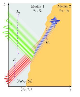
Fig. 1: Spacetime scattering at an arbitrarily accelerated interface. The subscripts i, r and t stand for incident, reflected and transmitted, while the subscripts $1$ and $2$ refer to the two media.

III.  Electromagnetic Scattering Solutions

A.  Analysis Problem

The incident wave may be written as

$$E_{\text{i}}=A_{\text{i}}f\left(k_{\text{i}}z-\omega_{\text{i}}t\right)\,,$$ (1)

where $f\left(\cdot\right)$ represents an arbitrary waveform profile. We subsequently apply the frame-hopping strategy [9, 10]: the electromagnetic fields, $\boldsymbol{E}$ and $\boldsymbol{H}$, are transformed into their comoving-frame counterparts, where we apply the stationary boundary conditions, and the resulting complete fields are transformed back to the laboratory frame. After some algebraic manipulations, we obtain the following result:

$$E_{\text{r}}=\frac{\eta_{2}-\eta_{1}}{\eta_{2}+\eta_{1}}\frac{1-n_{1}\beta\left(t\right)}{1+n_{1}\beta\left(t\right)}A_{\text{i}}\,f\left(\frac{1-n_{1}\beta\left(t\right)}{1+n_{1}\beta\left(t\right)}\left(k_{\text{i}}z+\omega_{\text{i}}t\right)\right)\,,$$ (2a)

$$E_{\text{t}}=\frac{2\eta_{2}}{\eta_{2}+\eta_{1}}\frac{1-n_{1}\beta\left(t\right)}{1-n_{2}\beta\left(t\right)}A_{\text{i}}\,f\left(\frac{1-n_{1}\beta\left(t\right)}{1-n_{2}\beta\left(t\right)}\left(k_{\text{i}}z-\omega_{\text{i}}t\right)\right)\,,$$ (2b)

where $$\beta\left(t\right)$$ is the velocity of the interface as a function of the laboratory time and is given by

$$\beta\left(t\right)=\frac{\beta_{0}\gamma_{0}+\int_{0}^{t}a\left(t_{1}\right)\,\differential{t_{1}}}{\sqrt{1+\left(\beta_{0}\gamma_{0}+\int_{0}^{t}a\left(t_{1}\right)\,\differential{t_{1}}\right)^{2}}}\,.$$ (2c)

Surprisingly, the derivation of Eqs. (2) does not require the explicit form of the coordinate transformation to the proper comoving frame: it turns out that the scattering coefficients in the moving frame can be expressed in terms of ratios of partial derivatives of the coordinate transformation, which ultimately obliterate the coordinate transformation.

B.  Synthesis Problem

The fact that the phase argument of the expressions in Eqs. (2) is a nonlinear function of time reveals that the scattered waves exhibit chirping when subjected to proper acceleration, as depicted in Fig. 1. This prompts an inverse problem: determining the velocity of the interface for achieving a specified chirping profile in the scattered waves. To unravel this, say for the transmitted wave, we must solve the instantaneous angular frequency equation [11],

$$\frac{1-n_{1}\beta\left(t\right)}{1-n_{2}\beta\left(t\right)}\omega_{\text{i}}=\omega_{\text{i}}+\varphi^{\prime}\left(t\right)\,,$$ (3)

with $\varphi\left(t\right)$ being the phase of the complex envelope of the wave, for the velocity $\beta\left(t\right)$, yielding the solution

$$\beta\left(t\right)=\frac{\varphi^{\prime}\left(t\right)}{n_{2}\varphi^{\prime}\left(t\right)+\left(n_{2}-n_{1}\right)\omega_{\text{i}}}\,.$$ (4)

If we consider a linear upward chirp

$$\varphi\left(t\right)=a\frac{t^{2}}{\alpha^{2}}\,,$$ (5)

where $a>0$ is the chirp parameter and $\alpha$ the width of the incident wave, the velocity profile [Eq. (4)] can be integrated to

$$z\left(t\right)=z_{0}+\frac{t}{n_{2}}+\frac{\left(n_{2}-n_{1}\right)\omega_{\text{i}}\alpha^{2}}{2an_{2}^{2}}\log\frac{\left(n_{2}-n_{1}\right)\omega_{\text{i}}\alpha^{2}}{\left(n_{2}-n_{1}\right)\omega_{\text{i}}\alpha^{2}+2an_{2}t}\,.$$ (6)

Figure 2 illustrates the synthesis result for the linear upward chirp [Eq. (5)] for $a=5$, where the incident waveform [Eq. (1)] is a Gaussian modulated pulse (Fig. 2(a)). The velocity of the interface is then obtained by inserting Eq. (5) into Eq. (4), while the chirped transmitted wave is obtained by inserting the so-obtained velocity into Eq. (2b). Figure 2(b) plots the trajectory of the interface [Eq. (6)] that produces the specific chirping profile of Eq. (5) in a spacetime diagram. The obtained interface profile, despite the complexity of the mathematical solution in Eq. (6), is not very complex because the chirp specification in Eq. (5) is fairly simple (linear chirp). However, the method is applicable to chirping profiles of arbitrary complexity.

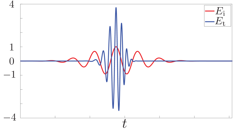
(a)

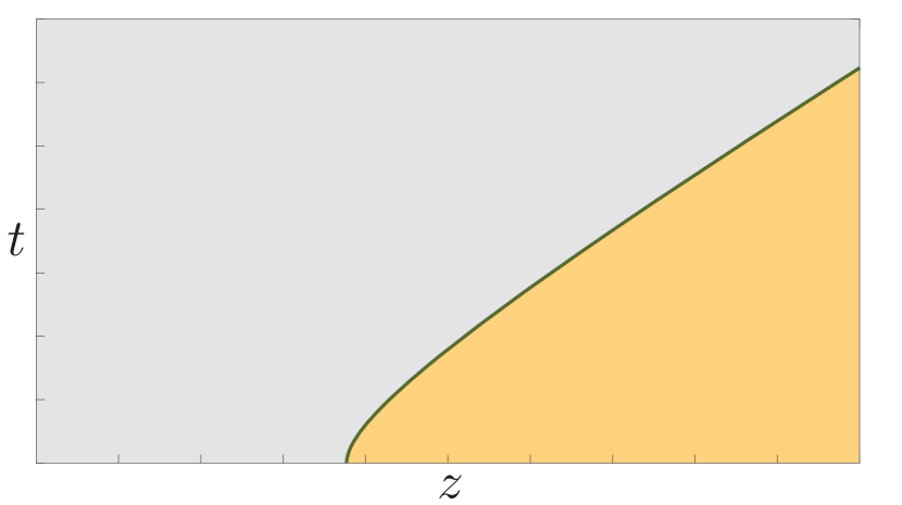
(b)

Fig. 2: Scattering at an accelerated modulated single interface with velocity in Eq. (4) for the chirping profile in Eq. (5) with chirp parameter $a=5$ and the electromagnetic parameters $n_{1}=1$, $n_{2}=3$ and $\eta_{1}=1=\eta_{2}$. (a) Incident Gaussian modulated pulse [Eq. (1)] and transmitted wave [Eq. (2b)]. (b) Trajectory of the interface [Eq. (6)] in a spacetime diagram.

References

- [1] C. Caloz and Z.-L. Deck-Léger, “Spacetime metamaterials–Part I: General concepts,” IEEE Trans. Antennas Propag., vol. 68, no. 3, pp. 1569–1582, 2019.
- [2] C. Caloz and Z.-L. Deck-Léger, “Spacetime metamaterials–Part II: Theory and applications,” IEEE Trans. Antennas Propag., vol. 68, no. 3, pp. 1583–1598, 2019.
- [3] C. Caloz, Z.-L. Deck-Léger, A. Bahrami, O. C. Vicente, and Z. Li, “Generalized space-time engineered modulation (GSTEM) metamaterials: A global and extended perspective.” IEEE Antennas Propag Mag., 2022.
- [4] C. Doppler, “Über das farbige Licht der Doppelsterne und einiger anderer Gestirne des Himmels,” Königl. Böhm Gedsellsch. d. Wis., vol 2, pp. 465–482, 1842.
- [5] A. Fresnel, “Lettre d’Augustin Fresnel à François Arago sur l’influence du mouvement terrestre dans quelques phénomènes d’optiques,” Ann. Chim. Phys., vol 9, pp. 57–66, 1818.
- [6] P. A. Huidobro, E. Galiffi, S. Guenneau, R. V. Craster, and J. Pendry, “Fresnel drag in space-time-modulated metamaterials,” Proc. Natl. Acad. Sci., vol. 116, no. 50, pp. 24 943–24 948, 2019.
- [7] Z.-L. Deck-Léger, N. Chamanara, M. Skorobogatiy, M. G. Silveirinha, and C. Caloz, “Uniform-velocity spacetime crystals,” Adv. Photonics, vol. 1, no. 5, p. 056002, 2019.
- [8] A. Bahrami, Z.-L. Deck-Léger, and C. Caloz, “Electrodynamics of accelerated-modulation space-time metamaterials,” Physical Review Applied, vol. 19, p.054044, 2023.
- [9] A. Bahrami, Z.-L. Deck-Léger Z. Li, and C. Caloz, “Generalized FDTD scheme for moving electromagnetic structures with arbitrary space-time configurations,” arXiv preprint arXiv:2306.10035, 2023.
- [10] J. Van Bladel, Relativity and Engineering, Springer Science & Business Media, 2012, vol. 15.
- [11] B. E. A. Saleh and M. C. Teich, Fundamentals of Photonics, 3th edition, New York: Wiley, 2019.