Classification Diffusion Models

Abstract

A prominent family of methods for learning data distributions relies on density ratio estimation (DRE), where a model is trained to classify between data samples and samples from some reference distribution. These techniques are successful in simple low-dimensional settings but fail to achieve good results on complex high-dimensional data, like images. A different family of methods for learning distributions is that of denoising diffusion models (DDMs), in which a model is trained to denoise data samples. These approaches achieve state-of-the-art results in image, video, and audio generation. In this work, we present Classification Diffusion Models (CDMs), a generative technique that adopts the denoising-based formalism of DDMs while making use of a classifier that predicts the amount of noise added to a clean signal, similarly to DRE methods. Our approach is based on the observation that an MSE-optimal denoiser for white Gaussian noise can be expressed in terms of the gradient of a cross-entropy-optimal classifier for predicting the noise level. As we illustrate, CDM achieves better denoising results compared to DDM, and leads to at least comparable FID in image generation. CDM is also capable of highly efficient one-step exact likelihood estimation, achieving state-of-the-art results among methods that use a single step. Code is available on the project’s webpage.

Figure 1: Samples from an unconditional CDM trained on CelebA $\mathbf{64\times 64}$ (left) and from a conditional CDM trained on CIFAR-10 (right). We introduce a diffusion based generative model that relies on a classifier for predicting the amount of white Gaussian noise added to clean samples. Our method relies on a theoretical relation between the optimal such classifier and the minimum-MSE denoiser for removing white Gaussian noise from samples.

1 Introduction

Denoising diffusion models (DDMs) (Sohl-Dickstein et al., 2015; Ho et al., 2020) have led to unprecedented success in generative modeling of complex high-dimensional data, from images (Dhariwal & Nichol, 2021; Rombach et al., 2022), audio excerpts (Kong et al., 2021; Chen et al., 2021; Jeong et al., 2021), and video clips (Girdhar et al., 2023; Bar-Tal et al., 2024), to protein structure (Watson et al., 2022; Qiao et al., 2022; Schneuing et al., 2022). This has made them perhaps the most prominent technique for learning data distributions in recent years, with applications in e.g. solving inverse problems (Kawar et al., 2022; Saharia et al., 2022), image editing (Meng et al., 2021; Hertz et al., 2022; Brooks et al., 2023; Huberman-Spiegelglas et al., 2023) and medical data enhancement (Song et al., 2023; Chung & Ye, 2022), to name just a few.

A more classical family of methods for learning data distributions relies on the concept of density-ratio estimation (DRE) (Sugiyama et al., 2012). DRE techniques transform the unsupervised task of learning the distribution of data into the supervised task of learning to classify between data samples and samples from some reference distribution (Gutmann & Hyvärinen, 2012; Ceylan & Gutmann, 2018; Rhodes et al., 2020; Choi et al., 2022). These methods attracted a lot of research efforts over the years (Lazarow et al., 2017; Grover & Ermon, 2018; Rhodes et al., 2020; Yair & Michaeli, 2023). However, to date, they have not achieved results comparable to diffusion models in settings involving complex high-dimensional data, like images.

DDMs are based on minimum-MSE (MMSE) denoising, while DRE methods hinge on optimal classification. In this work, we show a connection between the optimal classifier for predicting the level of white Gaussian noise added to a data sample, and the MMSE denoiser for cleaning such noise. Specifically, we show that the latter can be obtained from the gradient of the former. Utilizing this connection, we propose classification diffusion model (CDM), a generative method that combines the formalism of DDMs, but instead of a denoiser, employs a noise-level classifier. Our CDM can be used to generate samples in an iterative manner, similarly to that used in DDMs.

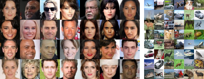
We illustrate through experiments that CDM is a more accurate denoiser, in terms of MSE, compared to a DDM with similar architecture, and is thus capable of generating images with slightly better FID. Representative generation examples are shown in Fig. 1. Furthermore, while DDMs require many neural function evaluations (NFEs) to calculate the likelihood-ELBO (Ho et al., 2020), or to approximate the exact likelihood using an ODE solver (Song et al., 2020c), CDM is inherently capable of outputting the exact log-likelihood in a single NFE. In fact, CDM achieves state-of-the-art negative-log-likelihood (NLL) results among methods that use a single NFE, and comparable results to computationally-expensive SDE-based methods.

2 Background

DDMs, first introduced by Sohl-Dickstein et al. (2015); Ho et al. (2020), are a class of generative models that sample from a learned target distribution by gradually denoising white Gaussian noise. More formally, DDMs generate samples by attempting to reverse a forward diffusion process with $T$ steps that starts from a data point ${\mathbf{x}}_{0}$ and evolves as ${\mathbf{x}}_{t}=\sqrt{\alpha_{t}}{\mathbf{x}}_{t-1}+\sqrt{1-\alpha_{t}}\tilde{\varepsilon_{t}}$, $t=1,\ldots,T$, where $\{\tilde{\varepsilon}_{t}\}$ are iid standard Gaussian vectors. Defining $\bar{\alpha}_{t}=\prod_{0}^{t}\alpha_{t}$, samples along this forward diffusion can be equivalently expressed as

$${\mathbf{x}}_{t}=\sqrt{\bar{\alpha}_{t}}{\mathbf{x}}_{0}+\sqrt{1-\bar{\alpha}_{t}}{\mathbf{\varepsilon}}_{t},\quad{\mathbf{\varepsilon}}_{t}\sim\mathcal{N}(0,\mathbf{I}),$$ (1)

where $\{\bar{\alpha}_{t}\}$ is a monotonic sequence such that $\alpha_{T}\approx 1$, which enforces the density $p_{{\mathbf{x}}_{T}}$ to be close to the normal distribution $\mathcal{N}(0,\mathbf{I})$.

The reverse diffusion process is learned by modeling the distributions of ${\mathbf{x}}_{t-1}$ given ${\mathbf{x}}_{t}$ as a Gaussian with mean

$$\mathbb{E}[{\mathbf{x}}_{t-1}|{\mathbf{x}}_{t}]=\frac{1}{\sqrt{\alpha_{t}}}\left({\mathbf{x}}_{t}-\frac{1-\alpha_{t}}{\sqrt{1-\bar{\alpha}_{t}}}\varepsilon_{\theta}({\mathbf{x}}_{t},t)\right)$$ (2)

and covariance $\sigma_{t}\mathbf{I}$, where $\varepsilon_{\theta}(\cdot,\cdot)$ is a neural network. Training is done by minimizing the ELBO loss, which reduces to a series of MSE terms,

$$\mathcal{L}=\sum_{t=1}^{T}\mathbb{E}_{{\mathbf{x}}_{0},{\mathbf{\varepsilon}}_{t}}\left[\lVert\varepsilon_{\theta}({\mathbf{x}}_{t},t)-{\mathbf{\varepsilon}}_{t}\rVert_{2}^{2}\right].$$ (3)

At convergence to the optimal solution, the neural network approximates the timestep-dependent posterior mean

$$\varepsilon_{\theta}({\bm{x}}_{t},t)=\mathbb{E}[{\mathbf{\varepsilon}}_{t}|{\mathbf{x}}_{t}={\bm{x}}_{t}].$$ (4)

To generate samples, DDMs sample ${\mathbf{x}}_{T}\sim\mathcal{N}(0,\mathbf{I})$ and then iteratively follow the learned reverse probabilities, terminating with a sample of ${\mathbf{x}}_{0}$. In more detail, at each timestep $t$, the model accepts ${\mathbf{x}}_{t}$ and outputs a prediction of the noise ${\mathbf{\varepsilon}}_{t}$ (equivalently, a prediction of the clean signal ${\mathbf{x}}_{0}$), from which ${\mathbf{x}}_{t-1}$ is obtained by sampling from the reverse distribution. The process described above is that underlying the DDPM method (Ho et al., 2020). Here we also experiment with DDIM (Song et al., 2020a) and DPMSolver (Lu et al., 2022), which follow a similar structure.

3 Method

Figure 2: A diagram of CDM (right) compared with DDM (left). DDM functions as an MSE denoiser conditioned on the noise level, whereas CDM operates as a classifier. Given a noisy image, CDM outputs a probability vector predicting the noise level, such that the $t$-th element in this vector is the probability that the noise level of the image corresponds to timestep $t$ in the diffusion. To obtain the clean image with CDM, the MMSE denoiser is obtained as the gradient of the probability vector w.r.t the input image, as stated in Theorem 3.1.

We start by deriving a relation between classification and denoising, and then use it as the basis for our CDM method.

Let the random vector ${\mathbf{x}}_{t}$ be defined as in (1) for timesteps $t\in\{1,\ldots,T\}$ and set an additional timestep $T+1$ to be pure Gaussian noise, i.e., ${\mathbf{x}}_{T+1}\sim\mathcal{N}(0,\mathbf{I})$. We denote the density of each ${\mathbf{x}}_{t}$ by $p_{{\mathbf{x}}_{t}}({\bm{x}})$. Our approach is based on training a classifier that takes as input a noisy sample ${\mathbf{x}}_{t}$ and predicts its timestep $t$. Formally, let t be a discrete random variable taking values in $\{1,\ldots,T+1\}$, with probability mass function $p_{\textnormal{t}}(t)=\mathbb{P}({\textnormal{t}}=t)$, and let the random vector $\tilde{{\mathbf{x}}}$ be the diffusion signal at a random timestep t, namely $\tilde{{\mathbf{x}}}={\mathbf{x}}_{{\textnormal{t}}}$. Note that the density of each ${\mathbf{x}}_{t}$ can be written as $p_{{\mathbf{x}}_{t}}({\bm{x}})=p_{\tilde{{\mathbf{x}}}|{\textnormal{t}}}({\bm{x}}|t)$ and the density of $\tilde{{\mathbf{x}}}$ is equal to

$$p_{\tilde{{\mathbf{x}}}}({\bm{x}})=\sum_{t=1}^{T+1}p_{{\mathbf{x}}_{t}}({\bm{x}})p_{\textnormal{t}}(t).$$ (5)

Given a sample ${\bm{x}}$ drawn from (5), we are interested in a classifier that outputs the probability vector $(p_{{\textnormal{t}}|\tilde{{\mathbf{x}}}}(1|{\bm{x}}),p_{{\textnormal{t}}|\tilde{{\mathbf{x}}}}(2|{\bm{x}}),\ldots,p_{{\textnormal{t}}|\tilde{{\mathbf{x}}}}(T+1|{\bm{x}}))$, where $p_{{\textnormal{t}}|\tilde{{\mathbf{x}}}}(t|{\bm{x}})=\mathbb{P}({\textnormal{t}}=t|\tilde{{\mathbf{x}}}={\bm{x}})$. As we now show, the denoiser in (4) corresponds to the gradient of this classifier.

Theorem 3.1.

For t, $\tilde{{\mathbf{x}}}$ and ${\mathbf{x}}_{t}$ as defined above, and denoting $F({\bm{x}},t)=\log(p_{{\textnormal{t}}|\tilde{{\mathbf{x}}}}(T+1|{\bm{x}}))-\log(p_{{\textnormal{t}}|\tilde{{\mathbf{x}}}}(t|{\bm{x}}))$, we have that

$$\mathbb{E}[{\mathbf{\varepsilon}}_{t}|{\mathbf{x}}_{t}={\bm{x}}_{t}]=\sqrt{1-\bar{\alpha}_{t}}(\nabla_{{\bm{x}}_{t}}F({\bm{x}}_{t},t)+{\bm{x}}_{t})$$ (6)

regardless of the choice of the probability mass function $p_{\textnormal{t}}$, provided that $p_{\textnormal{t}}(t)>0$ for all $t\in\{1,...,T+1\}$.

The proof, provided in App. A.1, relies on Tweedie’s formula (Miyasawa et al., 1961; Stein, 1981; Efron, 2011).

Algorithm 1 CDM Training

0:  Dataset of training samples $\mathcal{D}$

1:  repeat

2:     ${\bm{x}}_{0}\sim\mathcal{D},\ t\sim U(\{1,\ldots,T+1\}),\ \varepsilon\sim\mathcal{N}(0,\mathbf{I})$

3:     ${\bm{x}}_{t}=\sqrt{\bar{\alpha}_{t}}{\bm{x}}_{0}+\sqrt{1-\bar{\alpha}_{t}}\varepsilon$

4:     $F_{\theta}({\bm{x}}_{t},t)=f_{\theta}({\bm{x}}_{t})[T+1]-f_{\theta}({\bm{x}}_{t})[t]$

5:     $\varepsilon_{\theta}({\bm{x}}_{t},t)=\sqrt{1-\bar{\alpha}_{t}}\left(\nabla_{{\bm{x}}_{t}}F_{\theta}({\bm{x}}_{t},t)+{\bm{x}}_{t}\right)$

6:     take gradient step on

7:              $\nabla_{\theta}(w_{ce}\cdot\mathcal{L}_{\text{CE}}(t,f_{\theta}({\bm{x}}_{t}))+\mathcal{L}_{\text{MSE}}(\varepsilon,\varepsilon_{\theta}({\bm{x}}_{t},t))$

8:  until converged

Algorithm 2 DDPM Sampling Using CDM

0:  Noise level classifier $f_{\theta}(\cdot)$

1:  sample ${\bm{x}}_{T}\sim\mathcal{N}(0,\mathbf{I})$

2:  for $t=T,\ldots,1$ do

3:     $F_{\theta}({\bm{x}}_{t},t)=f_{\theta}({\bm{x}}_{t})[T+1]-f_{\theta}({\bm{x}}_{t})[t]$

4:     $\varepsilon_{\theta}({\bm{x}}_{t},t)=\sqrt{1-\bar{\alpha}_{t}}\left(\nabla_{{\bm{x}}_{t}}F_{\theta}({\bm{x}}_{t},t)+{\bm{x}}_{t}\right)$

5:     sample $z\sim\mathcal{N}(0,\mathbf{I})$ if $t>1$, else set $z=0$

6:     ${\bm{x}}_{t-1}=\frac{1}{\sqrt{\alpha_{t}}}\left({\bm{x}}_{t}-\frac{1-\alpha_{t}}{\sqrt{1-\bar{\alpha}_{t}}}\varepsilon_{\theta}({\bm{x}}_{t},t)\right)+\sigma_{t}z$

7:  end for

8:  return ${\bm{x}}_{0}$

Theorem 3.1 suggests that we may replace the denoiser used in DDM by a classifier, as illustrated in Fig. 2, and use any desired sampling method (e.g. DDPM, DDIM, etc.). However, as we show in Sec. 4.2, naively training such a classifier with the standard cross-entropy (CE) loss, leads to poor results. This is because a classifier may reach good classification accuracy (and a low CE loss) even without having its gradient precisely satisfy the property (6). In such a case, the classifier does not serve as an MMSE denoiser of sufficient quality for image generation.

To circumvent this effect, we suggest training the classifier with a combination of a CE loss on its outputs, and an MSE loss on its gradient, according to the relation (6). The network’s gradient can be obtained using automatic-differentiation. Following Ho et al. (2020), we use the same weight for all timesteps in the MSE loss. Our full training algorithm is described in Algorithm 1. Algorithm 2 shows how to generate samples with CDM using the DDPM sampler. A similar approach can be used with other samplers.

As we show in Sec. 4, the combination of the CE and MSE losses not only leads to better performance than using only CE, as in DRE methods, but also leads to better performance than using only MSE, as in DDMs. We further show that this approach outperforms pre-trained DDMs (with similar architectures to our CDM).

Note from Algorithm 2 that each step $t$ in DDPM sampling using CDM is given by

$${\bm{x}}_{t-1}=\sqrt{\alpha_{t}}{\bm{x}}_{t}-\frac{1-\alpha_{t}}{\sqrt{\alpha_{t}}}\nabla_{{\bm{x}}_{t}}F_{\theta}({\bm{x}}_{t},t)+\sigma_{t}z,$$ (7)

where $z\sim\mathcal{N}(0,\mathbf{I})$. Now, since $F_{\theta}({\bm{x}}_{t},t)$ is given by $f_{\theta}({\bm{x}}_{t})[T+1]-f_{\theta}({\bm{x}}_{t})[t]$, each step in fact steers the process in the direction that maximizes the probability of noise level $t$, while minimizing the probability of noise level $T+1$. This can be thought of as taking a gradient step with size $\frac{1-\alpha_{t}}{\sqrt{\alpha_{t}}}$, followed by a step in a random exploration direction with magnitude $\sigma_{t}$, similarly to Langevin dynamics.

Figure 3: Analytical Example of Log Likelihood. The illustrated densities represent uniform distributions $U\left[-\frac{\gamma}{2},\frac{\gamma}{2}\right]^{3\times 32\times 32}$ for each $\gamma$ value in the set $\{0.25,0.5,1,2,3\}$. Samples from these distributions correspond to images of iid uniform noise. The red points on the graph indicate the estimated likelihood results obtained from CDM models trained on samples from each distribution. The alignment of these points along the diagonal serves as evidence supporting our likelihood estimation as per Theorem 3.2.

3.1 Exact Likelihood Calculation in a Single Step

To compute the likelihood of a given sample, DDMs are required to either perform a complete reverse process in order to compute a lower bound on the log likelihood using the ELBO (Ho et al., 2020), or can approximate the exact likelihood (Song et al., 2020c) using an ODE solver based on repeated evaluations of the network. In contrast, a CDM is able to calculate the exact likelihood in a single NFE. In fact, a CDM can compute the likelihood w.r.t. the distribution $p_{{\mathbf{x}}_{t}}$ of noisy images, for any desired timestep $t$. Specifically, we have the following (see proof in App. A.3).

Theorem 3.2.

For any $t\in\{1,\ldots,T+1\}$,

$$p_{{\mathbf{x}}_{t}}({\bm{x}})=\frac{p_{\textnormal{t}}(T+1)}{p_{\textnormal{t}}(t)}\,\frac{p_{{\textnormal{t}}|\tilde{{\mathbf{x}}}}(t|{\bm{x}})}{p_{{\textnormal{t}}|\tilde{{\mathbf{x}}}}(T+1|{\bm{x}})}\,\mathcal{N}({\bm{x}};0,\mathbf{I}).$$ (8)

Note that the first term in (8) only depends on the pre-selected probability mass function $p_{\textnormal{t}}$ (which we choose to be uniform in our experiments), and the second term can be obtained from the $t$-th and $(T+1)$-th entries of the vector at the output of the CDM classifier (after applying softmax). This implies that we can calculate the likelihood of any given image ${\bm{x}}$ w.r.t. to the density $p_{{\mathbf{x}}_{t}}$ of noisy images for any noise level $t$. In particular, recall that $\bar{\alpha}_{1}\approx 1$, so that from (1), $p_{{\mathbf{x}}_{1}}$ is approximately the density of clean images. Thus, by choosing $t=1$, we can calculate the log likelihood of clean images.

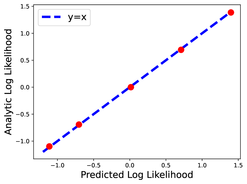
We validate our efficient likelihood computation by applying it to toy examples with known densities, allowing us to compute the analytical likelihood and verify that our computations align with theoretical expectations. We select several distributions of iid uniform noise, each with a different support. We train CDM individually for each density following the procedure outlined in Algorithm 1. Further details can be found in App. C. Figure 3 illustrates the calculated likelihood compared to the theoretical value for each distribution. The close alignment between our results and the ground-truth underscores the effectiveness of our model in learning the density from which the data was sampled.

Table 1: Image generation quality. We compare the FID (lower is better) achieved by DDM and CDM using several sampling schemes for CelebA, unconditional CIFAR-10 and conditional CIFAR-10 (for which we train a DDM on our own, as no model in the original implementation (Ho et al., 2020) supports CFG).

Sampling Method

Model

CelebA $64\times 64$	DDM	CDM
DDIM Sampler, 50 steps	8.47	4.78
DDPM Sampler, 1000 steps	4.13	2.51
2nd order DPM Solver, 25 steps	6.16	4.45

Unconditional CIFAR-10 $32\times 32$	DDM	CDM
DDIM Sampler, 50 steps	7.19	7.56
DDPM Sampler, 1000 steps	4.77	4.74
2nd order DPM Solver, 25 steps	6.91	7.29

Conditional CIFAR-10 $32\times 32$	DDM	CDM
DDIM Sampler, 50 steps	5.92	5.08
DDPM Sampler, 1000 steps	4.70	3.66
2nd order DPM Solver, 25 steps	5.87	4.87

Table 2: NLL (bits/dim) calculated on CIFAR-10 test-set. For each model we list the NFEs required for calculating the NLL.

Model	NLL $\downarrow$	NFE
iResNet (Behrmann et al., 2019)	3.45	100
FFJORD (Grathwohl et al., 2018)	3.40	$\sim$3K
MintNet (Song et al., 2019)	3.32	120
FlowMatching (Lipman et al., 2022)	2.99	142
VDM (Kingma et al., 2021)	2.65	10K
DDPM ($L$) (Ho et al., 2020)	$\leq$3.70	1K
DDPM ($L_{simple}$) (Ho et al., 2020)	$\leq$3.75	1K
DDPM (SDE) (Song et al., 2020c)	3.28	$\sim$200
DDPM++ cont. (Song et al., 2020c)	2.99	$\sim$200
RealNVP (Dinh et al., 2016)	3.49	1
Glow (Kingma & Dhariwal, 2018)	3.35	1
Residual Flow (Chen et al., 2019)	3.28	1
CDM	3.38	1
CDM(unif.)	2.98	1

Figure 4: Denoising results for CelebA $\mathbf{64\times 64}$ at various noise levels. We show a comparison between CDM and a pre-trained DDM for different noise levels. The right column shows CDM and DDM predictions for pure Gaussian noise. When an MMSE denoiser is given pure noise as input, it should theoretically predict the expectation of the prior distribution. As observed, DDM outputs a highly noisy image, whereas CDM generates an image much closer to the mean of the dataset.

Figure 5: MSE-based denoising results across different noise levels (timesteps $t$). In terms of MSE, our method significantly outperforms a pre-trained DDM with the same architecture, at high noise levels, while demonstrating comparable performance at low to mid-range noise levels.

4 Experiments

We train several models using CDM on two common datasets. For CIFAR-10 $32\times 32$ (Krizhevsky et al., 2009) we train both a class conditional model and an unconditional model. We also train a similar model for CelebA (Liu et al., 2015), using face images of size $64\times 64$. We compare our method with pre-trained DDMs with similar architecture and hyperparameter choices, to disentangle the benefits of our method from other variables. Specifically, for CDM we alter the last two layers such that the output is a vector of logits, facilitating training following Algorithm 1. We additionally remove all timestep conditioning layers. These changes have a negligible impact on the number of parameters in the model. For more details please refer to App. B. We evaluate the performance of CDM as an MMSE denoiser, for image generation using FID (Heusel et al., 2017), and on negative log likelihood (NLL) estimations of the data.

(a) Comparison of the log probability of a single prediction between a model trained only using CE and a model trained using CE and MSE. The probability predicted by both models peaks near the correct timestep, but the model trained with MSE produces probabilities that decay faster for further time steps. Since the SoftMax operator is invariant to an additive factor, we subtract the maximal value from the vector (i.e., $f_{\theta}({\bm{x}}_{t})\leftarrow f_{\theta}({\bm{x}}_{t})-\max(f_{\theta}({\bm{x}}_{t}))$) for visualization.

(b) Confusion matrices evaluated for models trained with both MSE and CE loss (top) and only with CE loss (bottom). The colors indicate the probabilities. The similarity between the confusion matrices underlines that CE loss alone is adequate for accurate predictions around the real noise level. This is also shown in Fig. (6(a))

Figure 6: Classification results for CelebA $\mathbf{64\times 64}$.

4.1 Image Quality and Negative Log Likelihood

Figure 1 shows images generated by our model from CelebA and unconditional CIFAR-10. CDM succeeds in learning the target distributions and samples diverse and high quality images. We compare the quality of images generated using CDM to images sampled from pre-trained DDMs trained according to (Ho et al., 2020). Image quality is assessed using 50k FID (Heusel et al., 2017) with the train-set. For both CDM and DDM models, we compare images sampled using several schedulers; DDPM (Ho et al., 2020), DDIM (Song et al., 2020a), and DPM-Solver (Lu et al., 2022) samplers, set with 1000, 50, and 25 timesteps for sampling, respectively. The results, shown in Table 1, demonstrate that CDM is at least comparable to pre-trained DDMs in image quality, outperforming them in most cases.

As classifier free guidance (Ho & Salimans, 2022) (CFG) has become the bedrock of conditional generation with diffusion models, we validate CDM’s ability to apply CFG in conditional sampling. The conditional CIFAR-10 FID results are also shown in Table 1. As expected, CFG improves the image quality beyond the unconditional results.

We calculate log-likelihoods and compare our NLL results to recent leading methods in Table 2. CDM demonstrates comparable performance on NLL estimation for CIFAR-10 compared to DDMs. Notably, CDM stands out as a more efficient method than existing ones, requiring only a single forward pass for NLL computation. Table 2 also includes CDM(unif.), as outlined below in Sec. 4.3. This version of our model, which is more suited for denisity-ratio estimation tasks, improves our NLL predictions and achieves state-of-the-art results among methods employing a single step.

Figure 7: Comparison of denoising between a model trained using only CE and one trained using both CE and MSE. We note that the denoising results for the model trained using CE alone are poor, but are better for high noise levels than for lower ones. This resonates with our conclusion that models trained only with CE are only accurate near the real noise level: As denoising with CDM relies on Theorem 3.1, we would expect deteriorating denoising quality the further the real noise level is from $T+1$, as $f_{\theta}({\bm{x}})[T+1]$ is always used for denoising.

4.2 Analysis of CDM as a Denoiser and as a Classifier

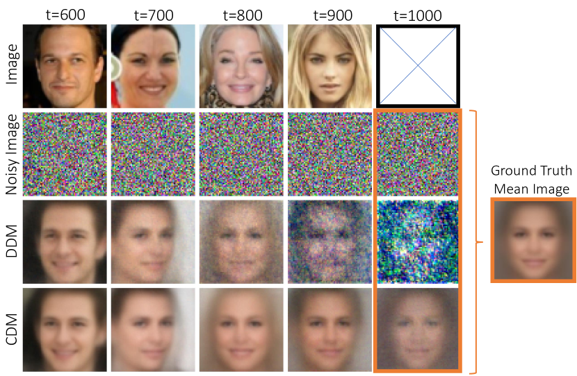
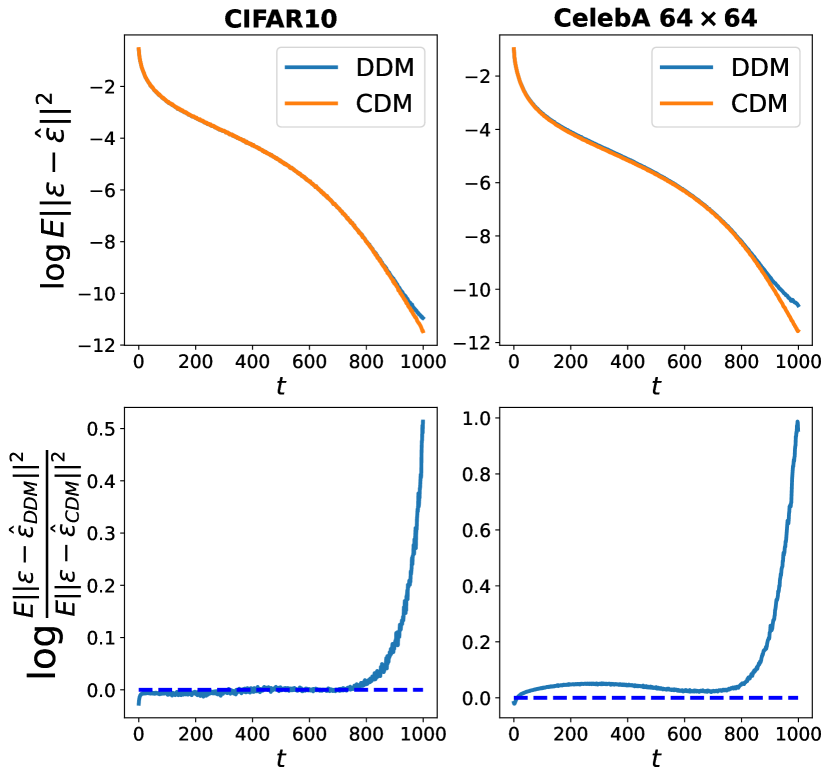
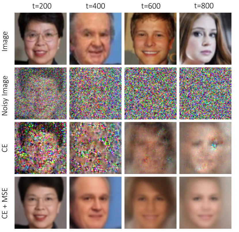
On the task of image denoising, CDM achieves better MSE than a pre-trained DDM of similar architecture at high noise levels and comparable MSE for low-mid noise levels, as we show in Fig. 5. These results are also reflected In Fig. 4, in which we show qualitative examples for image denoising of different noise levels.

In Theorem 3.1, we established that the MMSE denoiser corresponds to the gradient ot the optimal classifier. Therefore, in theory it should be sufficient to optimize only one of the objectives, i.e. either use only a CE loss on the model’s output or use only an MSE loss on its derivative. In Table 3 we report the MSE, CE and classification accuracy achieved by models trained with different losses. We emphasize that the model trained using only MSE in this comparison, is a CDM model trained using Algorithm 1, and is not equivalent to a DDM model trained following (3). As evident from Table 3, when using only the CE loss, the MSE is high, and when using only the MSE loss the CE and classification accuracy are poor.

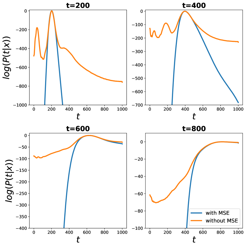
Figure 6(a) shows the prediction of the logits ($f_{\theta}({\bm{x}}_{t})$) for noisy images with different noise levels, comparing a model trained using CE to a model trained with both CE and MSE. A model trained using only the MSE loss is omitted from Fig. 6(a) because it fails to function as a classifier, as demonstrated by the accuracy column in Table 3. As the results in Fig. 6(a) reflect, in both scenarios the prediction near the true label is the same, namely the CE works well in the local area of the correct noise level. However, the model trained without MSE displays significantly higher predicted logits for more distant noise levels compared to its counterpart model. Moreover, the logits of the model trained without MSE do not decrease monotonically as the distance from the actual noise level increases, in contrast to the expected behavior. This emphasizes the importance of the MSE loss for obtaining good prediction globally.

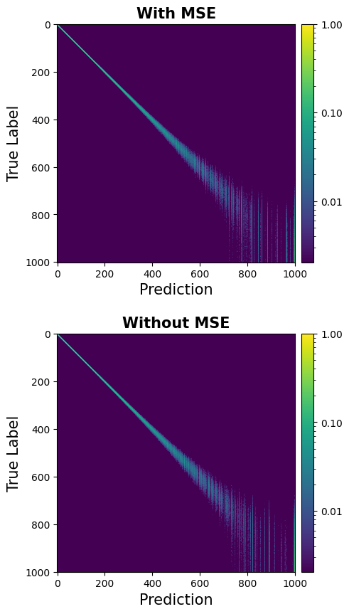
To assess the classifier’s performance, we present the confusion matrices of models trained with and without MSE loss in Figure 6(b). Notably, at lower noise levels, the classifier exhibits high confidence, while at higher noise levels, confidence diminishes. This finding corresponds to the DDPM scheduler (Ho et al., 2020), which partitions the noise levels to be more concentrated for high timesteps and less concentrated for low timesteps.

Figure 7 provides further qualitative analysis of the effect of training with different losses on the quality of the model’s image denoising capabilities. The results illustrate that the model trained using only CE loss achieves poor denoising quality compared to the CDM model trained with both CE and MSE.

4.3 Uniform Noise Scheduling for Better Likelihood Estimation

Table 3: The importance of using both losses in CDM. We demonstrate the importance of using both the CE and MSE losses at training. As can be seen, the best results are achieved when combining the losses. We report the results for CIFAR-10 test-set. FID is reported on 50k samples which were generated using DDIM scheduler with 50 steps. As shown by Rhodes et al. (2020), to avoid the density-chasm problem, the classification problem should be sufficiently hard to not be trivial, leading to low accuracy results.

Training	Acc $\uparrow$	CE $\downarrow$	MSE $\downarrow$	FID $\downarrow$	NLL $\downarrow$
Loss
CE	6.97$\%$	4.4931	0.2254	329	8.27
MSE	0$\%$	1659	0.0287	7.65	9.32
Both	8.34$\%$	4.3709	0.0287	7.56	3.38

Figure 8: Confusion matrix CDM(unif.) model evaluated on unconditional CIFAR-10 $\mathbf{32\times 32}$ using the scheduler from TDR. The colors indicate the probabilities. In contrast to DDPM noise scheduler, with TDR noise scheduler, the classification difficulty is preserved across all timesteps.

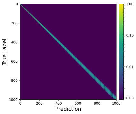
To see the effect of using a timestep scheduler tuned for DRE tasks, we repeat the CIFAR $32\times 32$ unconditional experiment, with a different noise scheduler. Following Rhodes et al. (2020) we use the scheduler defined as $\sqrt{1-\bar{\alpha}_{t}}=\frac{t}{T+1}$ and choose $T=1000$ similarly to our previous experiments. In Fig. 8, we illustrate that this scheduler induces a uniform difficulty in classification across various noise levels. This is in contrast to the DDM scheduler, depicted in Fig. 6(b), in which the classification difficulty increases with the noise level. Utilizing this scheduler, we achieve a state-of-the-art single-step NLL of 2.98 at the expense of a higher FID of 10.28 (using the DDIM sampler with 50 steps). This trade-off highlights that the scheduler optimal for learning the data distribution may not be ideal for sampling. Future research endeavors could explore schedulers aimed at further enhancing the NLL.

5 Related Work

Using the concept of DRE for learning distributions of data was initially studied by Gutmann & Hyvärinen (2012). Their noise contrastive estimation (NCE) method approximates the ratio between the density of the data distribution and that of white Gaussian noise. However, it struggles in practical scenarios where the gap between these distributions is large, as is the case for natural images (Rhodes et al., 2020). Conditional noise contrastive estimation (CNCE) (Ceylan & Gutmann, 2018) is a slightly improved version of NCE, in which the classification problem is designed to be harder. Specifically, CNCE is based on training a classifier to predict the order of a pair of samples with closer densities, e.g. achieved by pairing a data sample with its noisy version.

Telescoping density-ratio (TDR), proposed by Rhodes et al. (2020), avoids direct classification between data and noise. Instead, it uses a gradual transition between those two distributions, and trains a classifiers to distinguish between samples from every pair of adjacent densities. Such a classifier learns the ratio between adjacent distributions, and the overall ratio between the data and noise distributions is computed by multiplying all intermediate ratios.

Extending this concept, (Choi et al., 2022) took the notion further by expanding from a finite set of intermediate densities to an infinite continuum. This was accomplished by establishing a link between the estimation of density ratios for infinitesimally close distributions and the principles of score matching (Kingma & Cun, 2010; Song & Ermon, 2019; Song et al., 2020b), and training a model to predict the time score $\frac{\partial}{\partial t}\log p_{{\mathbf{x}}_{t}}$. In contrast, we draw a different connection which shows that an MMSE denoiser can be obtained as the gradient of an optimal noise level classifier. Also, to obtain the log ratio between the target and reference distributions, (Choi et al., 2022) needs to solve an integral over the time-score using an ODE solver, while in our method this ratio can be calculated in a single NFE.

Yair & Michaeli (2023) expanded the concept of TDR, proposing the training of a single noise level classifier instead of training a distinct classifier for each pair of neighboring densities. While this method is conceptually similar to ours, our approach distinguishes itself by incorporating the MSE loss as outlined in Theorem 3.1. As demonstrated in our experiments, this proves to be crucial for achieving high-quality image generation and accurate probability prediction.

6 Limitations and Conclusion

While CDM achieves high-quality results, it requires computing the network’s gradient, which leads to slow training and sampling. It may be possible to employ a smaller architecture with CDM, accelerating computation and reducing memory. For instance, by using only the encoder layers of the UNet (Ronneberger et al., 2015) for noise-level predictions, the upsampling effect would be emulated by the gradient operation. We leave this architecture search for future work.

We proved a relation between the optimal noise level classifier and the MMSE denoiser. Using this relation, we proposed a training algorithm, relying on both classification and regression losses. We demonstrated thorough experiments that training with the CE loss provides a reliable approximation for the probability of the correct noise level and its immediate neighbors. However, it falls short in approximating the probability of more distant neighbors. On the other hand, incorporating the MSE loss on the classifier gradient, as detailed in Theorem 3.1, results in a robust approximation, even for more distant neighbors. We validated our model’s performance compared to pre-trained DDMs, by quantifying the MSE denoising capabilities across all timesteps, as well as measuring the quality of images generated with our method. Finally, we demonstrated that CDM attains state-of-the-art NLL on the CIFAR-10 test-set among models that compute NLL in a single step. We illustrated the trade-off between a scheduler well-suited for sampling and one well-suited for likelihood estimation. We leave it for future work to further explore schedulers that optimize the NLL.

7 Potential Broader Impact

This paper presents work whose goal is to advance the field of Machine Learning and Generative Models. There are many potential societal consequences of our work, none which we feel must be specifically highlighted here.

Appendix A Proofs

A.1 Theorem 3.1 Proof

Using Bayes rule,

$$p_{{\mathbf{x}}_{t}}({\bm{x}})=p_{\tilde{{\mathbf{x}}}|{\textnormal{t}}}({\bm{x}}|t)=\frac{p_{{\textnormal{t}}|\tilde{{\mathbf{x}}}}(t|{\bm{x}})p_{\tilde{{\mathbf{x}}}}({\bm{x}})}{p_{\textnormal{t}}(t)}.$$ (9)

In particular, for $t=T+1$, this relation reads

$$p_{{\mathbf{x}}_{T+1}}({\bm{x}})=\frac{p_{{\textnormal{t}}|\tilde{{\mathbf{x}}}}(T+1|{\bm{x}})p_{\tilde{{\mathbf{x}}}}({\bm{x}})}{p_{\textnormal{t}}(T+1)}.$$ (10)

Combining (9) and (10) yields

$$p_{{\mathbf{x}}_{t}}({\bm{x}})=\frac{p_{\textnormal{t}}(T+1)}{p_{\textnormal{t}}(t)}\,\frac{p_{{\textnormal{t}}|\tilde{{\mathbf{x}}}}(t|{\bm{x}})}{p_{{\textnormal{t}}|\tilde{{\mathbf{x}}}}(T+1|{\bm{x}})}\,p_{{\mathbf{x}}_{T+1}}({\bm{x}}).$$ (11)

Taking the logarithm of both sides, we have

$$\log(p_{{\mathbf{x}}_{t}}({\bm{x}}))=\log\left(\frac{p_{\textnormal{t}}(T+1)}{p_{\textnormal{t}}(t)}\right)+\log\left(\frac{p_{{\textnormal{t}}|\tilde{{\mathbf{x}}}}(t|{\bm{x}})}{p_{{\textnormal{t}}|\tilde{{\mathbf{x}}}}(T+1|{\bm{x}})}\right)+\log(p_{{\mathbf{x}}_{T+1}}({\bm{x}})).$$ (12)

Taking the gradient of both sides w.r.t ${\bm{x}}$, and noting that the first term on the right hand side does not depend on ${\bm{x}}$, we get that

$$\nabla_{\bm{x}}\log(p_{{\mathbf{x}}_{t}}({\bm{x}}))=\nabla_{\bm{x}}\log(p_{{\textnormal{t}}|\tilde{{\mathbf{x}}}}(t|{\bm{x}}))-\nabla_{\bm{x}}\log(p_{{\textnormal{t}}|\tilde{{\mathbf{x}}}}(T+1|{\bm{x}}))+\nabla_{\bm{x}}\log(p_{{\mathbf{x}}_{T+1}}({\bm{x}})).$$ (13)

Since that $p_{{\mathbf{x}}_{T+1}}({\bm{x}})=\mathcal{N}(0,\mathbf{I})$, we have that $\nabla_{\bm{x}}\log(p_{{\mathbf{x}}_{T+1}}({\bm{x}}))=-{\bm{x}}$. Therefore, overall we have

$$\nabla_{\bm{x}}\log(p_{{\mathbf{x}}_{t}}({\bm{x}}))=\nabla_{\bm{x}}\log(p_{{\textnormal{t}}|\tilde{{\mathbf{x}}}}(t|{\bm{x}}))-\nabla_{\bm{x}}\log(p_{{\textnormal{t}}|\tilde{{\mathbf{x}}}}(T+1|{\bm{x}}))-{\bm{x}}.$$ (14)

As for the left hand side, since ${\mathbf{x}}_{t}=\sqrt{\bar{\alpha}_{t}}{\mathbf{x}}_{0}+\sqrt{1-\bar{\alpha}_{t}}{\mathbf{\varepsilon}}_{t}$ and ${\mathbf{\varepsilon}}_{t}\sim\mathcal{N}(0,\mathbf{I})$, using Tweedie’s formula (Miyasawa et al., 1961; Stein, 1981; Efron, 2011) it can be shown that

$$\nabla_{\bm{x}}\log(p_{{\mathbf{x}}_{t}}({\bm{x}}))=-\frac{1}{\sqrt{1-\bar{\alpha}_{t}}}\mathbb{E}[{\mathbf{\varepsilon}}_{t}|{\mathbf{x}}_{t}={\bm{x}}].$$ (15)

For completeness we provide the full proof for (15) in App. A.2. Substituting (14) into (15) and multiplying both sides by $\sqrt{1-\bar{\alpha}_{t}}$ gives

$$\mathbb{E}[{\mathbf{\varepsilon}}|{\mathbf{x}}_{t}={\bm{x}}]=\sqrt{1-\bar{\alpha}_{t}}\left(\nabla_{\bm{x}}\log(p_{{\textnormal{t}}|\tilde{{\mathbf{x}}}}(T+1|{\bm{x}}))-\nabla_{\bm{x}}\log(p_{{\textnormal{t}}|\tilde{{\mathbf{x}}}}(t|{\bm{x}}))+{\bm{x}}\right),$$ (16)

which completes the proof.

Note that the proof is correct for any choice of $p_{\textnormal{t}}$ (provided that $p_{\textnormal{t}}(t)>0$ for all $t$), since the term that depends on $p_{\textnormal{t}}$ does not depend on ${\bm{x}}$ and thus drops when taking the gradient. In practice, as mentioned in the main text, we chose to use ${\textnormal{t}}\sim U(\{1,...,T+1\})$.

A.2 Proof of Tweedie’s Formula for the Variance Preserving Case

Let us show that if ${\mathbf{x}}_{t}=\sqrt{\bar{\alpha}_{t}}{\mathbf{x}}_{0}+\sqrt{1-\bar{\alpha}_{t}}{\mathbf{\varepsilon}}_{t}$ and ${\mathbf{\varepsilon}}_{t}\sim\mathcal{N}(0,\mathbf{I})$ then $\nabla_{\bm{x}}\log(p_{{\mathbf{x}}_{t}}({\bm{x}}))=-\frac{1}{\sqrt{1-\bar{\alpha}_{t}}}\mathbb{E}[{\mathbf{\varepsilon}}_{t}|{\mathbf{x}}_{t}={\bm{x}}]$. Note that in this case

$$p_{{\mathbf{x}}_{t}}({\bm{x}}_{t}) =\int p_{{\mathbf{x}}_{t}|{\mathbf{x}}_{0}}({\bm{x}}_{t}|{\bm{x}}_{0})p_{{\mathbf{x}}_{0}}({\bm{x}}_{0})d{\bm{x}}_{0}$$

$$=\int\frac{1}{(2\pi)^{d/2}(1-\bar{\alpha}_{t})^{d/2}}\exp\left\{-\frac{1}{2(1-\bar{\alpha}_{t})}\lVert{\bm{x}}_{t}-\sqrt{\bar{\alpha}_{t}}{\bm{x}}_{0}\rVert^{2}\right\}p_{{\mathbf{x}}_{0}}({\bm{x}}_{0})d{\bm{x}}_{0}.$$ (17)

Taking the gradient w.r.t. ${\bm{x}}_{t}$ gives

$$\nabla_{{\bm{x}}_{t}}p_{{\mathbf{x}}_{t}}({\bm{x}}_{t}) =\int-\frac{1}{1-\bar{\alpha}_{t}}({\bm{x}}_{t}-\sqrt{\bar{\alpha}_{t}}{\bm{x}}_{0})\frac{1}{(2\pi)^{d/2}(1-\bar{\alpha}_{t})^{d/2}}\exp\left\{-\frac{1}{2(1-\bar{\alpha}_{t})}\lVert{\bm{x}}_{t}-\sqrt{\bar{\alpha}_{t}}{\bm{x}}_{0}\rVert^{2}\right\}p_{{\mathbf{x}}_{0}}({\bm{x}}_{0})d{\bm{x}}_{0}$$

$$=\int-\frac{1}{1-\bar{\alpha}_{t}}({\bm{x}}_{t}-\sqrt{\bar{\alpha}_{t}}{\bm{x}}_{0})p_{{\mathbf{x}}_{t}|{\mathbf{x}}_{0}}({\bm{x}}_{t}|{\bm{x}}_{0})p_{{\mathbf{x}}_{0}}({\bm{x}}_{0})d{\bm{x}}_{0}$$

$$=\int-\frac{1}{1-\bar{\alpha}_{t}}({\bm{x}}_{t}-\sqrt{\bar{\alpha}_{t}}{\bm{x}}_{0})p_{{\mathbf{x}}_{0}|{\mathbf{x}}_{t}}({\bm{x}}_{0}|{\bm{x}}_{t})p_{{\mathbf{x}}_{t}}({\bm{x}}_{t})d{\bm{x}}_{0}.$$ (18)

Dividing both sides by $p_{{\mathbf{x}}_{t}}({\bm{x}}_{t})$, we get

$$\nabla_{{\bm{x}}_{t}}\log p_{{\mathbf{x}}_{t}}({\bm{x}}_{t}) =\int-\frac{1}{1-\bar{\alpha}_{t}}({\bm{x}}_{t}-\sqrt{\bar{\alpha}_{t}}{\bm{x}}_{0})\,p_{{\mathbf{x}}_{0}|{\mathbf{x}}_{t}}({\bm{x}}_{0}|{\bm{x}}_{t})d{\bm{x}}_{0}$$

$$=\int-\frac{1}{\sqrt{1-\bar{\alpha}_{t}}}\,{\mathbf{\varepsilon}}_{t}\,p_{{\mathbf{x}}_{0}|{\mathbf{x}}_{t}}({\bm{x}}_{0}|{\bm{x}}_{t})d{\bm{x}}_{0}$$

$$=-\frac{1}{\sqrt{1-\bar{\alpha}_{t}}}\mathbb{E}[{\mathbf{\varepsilon}}_{t}|{\mathbf{x}}_{t}={\bm{x}}_{t}],$$ (19)

completing the proof.

A.3 Proof of Theorem 3.2

Substituting $p_{{\mathbf{x}}_{T+1}}({\bm{x}})=\mathcal{N}({\bm{x}};0,\mathbf{I})$ into (11) leads to

$$p_{{\mathbf{x}}_{t}}({\bm{x}})=\frac{p_{\textnormal{t}}(T+1)}{p_{\textnormal{t}}(t)}\,\frac{p_{{\textnormal{t}}|\tilde{{\mathbf{x}}}}(t|{\bm{x}})}{p_{{\textnormal{t}}|\tilde{{\mathbf{x}}}}(T+1|{\bm{x}})}\,\mathcal{N}({\bm{x}};0,\mathbf{I}),$$ (20)

which proves Theorem 3.2.

Appendix B Implementation details

B.1 Architectures

For fair comparison, for each dataset we used the same architecture for our method and for DDMs. As baslines we took the pre-trained model for CelebA $64\times 64$ from the DDIM Official Github (Song et al., 2020a) and the EMA pre-trained model for CIFAR-10 from the pytorch diffusion repository, who converted the pre-trained model from the Official DDPM implementation from tensorflow to pytorch.

For conditional CIFAR-10 we trained the DDM model by ourselves because there exist no pre-trained models for CIFAR-10 capable of handling CFG. We used the same architecture from (Ho et al., 2020) for both models and trained them for the same number of iterations (more details are in App. B.2.2). To condition the model on the class label, we learned an embedding for each class using nn.Embeding and injected it at all points where the time embedding was injected in the original architecture (for DDM we added it to the time embedding and for CDM we replaced the time embedding by the class embedding).

In contrast to DDM architectures, our model does not need the layers that process the timestep input so we removed them. In addition, our model outputs a probability vector in contrast to DDMs which output an image, therefore, we replaced the last convolution layer that reduces the number of channels to 3 in the original architecture by a convolution layers outputs 1024 and 512 channels for CelebA $64\times 64$ and CIFAR-10, respectively. Following this layer, we performed global average pooling and added a linear layer with an output dimension of $T+1$. The resulting change in the number of parameters is negligible.

As suggested by Yair & Michaeli (2023), we added a non-learned linear transformation at the output of the network, which performs cumulative-summation (cumsum). This enforces (for the optimal classifier) the $t$-th output of the model before this layer to be $\log r_{t}({\bm{x}})=\log\frac{p_{t}({\bm{x}})}{p_{t-1}({\bm{x}})}=\log p_{t}({\bm{x}})-\log p_{t-1}({\bm{x}})$ for $t\neq 1$ and $r_{1}({\bm{x}})=\log p_{1}({\bm{x}})$, so that after the cumsum layer, the $t$-th output is $\sum_{i=1}^{t}\log r_{i}({\bm{x}})=\log p_{t}({\bm{x}})$.

B.2 Hyperparamters

B.2.1 CelebA $64\times 64$

We trained the model for 500k iterations with a learning rate of $1\cdot 10^{-4}$. We started with a linear warmup of 5k iterations and reduced the learning rate by a factor of 10 after every 200k iterations. The typical value of the CE loss after convergence was $\sim 3.8$ while the MSE loss was $\sim 0.0134$ so we chose to give the CE loss a weight of $0.001$ to ensure the values of both losses have the same order of magnitude. In addition We used EMA with a factor of 0.9999, as done in the baseline model.

B.2.2 Unconditional and Conditional CIFAR-10

We trained the model for 500k iterations with a learning-rate of $2\cdot 10^{-4}$. We started with a linear warmup of 5k iterations and reduced the learning rate by a factor of 10 after every 200k iterations. The typical value of the CE loss after convergence was $\sim 4.4$ while the MSE loss was $\sim 0.03$ so we chose to give the CE loss a weight of $0.001$ to maintain values at the same order of magnitude. In addition, we used EMA with a factor of 0.9999, as done in the baseline model.

For the CDM(unif.) model we used the same hyperparametes except for learning rate, which we set to $1\cdot 10^{-4}$.

B.3 Data Augmentation

Following the models to which we compared, for all the datasets we normalized the images to the range $[-1,1]$ and applied random horizontal flip at training.

B.4 Classifier Free Guidance

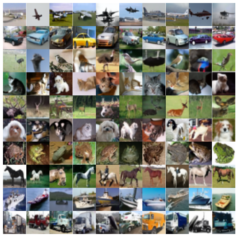
We used CFG to sample conditioned examples in Sec. 4.1 following (Ho & Salimans, 2022). We trained our own conditional models on the CIFAR-10 dataset, both for DDM and for CDM, and used label dropout of $0.1$. We selected the best parameter $w$ for each method using a grid search over $w=0.25,0.5,0.75,1$. In Fig. 9 we show samples from the conditional model. Each row corresponds to a different class.

B.5 The Addition of Timestep $T+1$

As outlined in Sec. 3, we introduce an additional timestep $x_{T+1}$ that is not present in DDMs. This inclusion is fundamental to our method formulation, as demonstrated in App. A.1. Importantly, this addition does not alter the number of sampling steps, as we continue initiating the reverse process from ${\textnormal{t}}=T$, following the approach in DDM. During training, we employ both MSE and CE losses for all timesteps, while the last timestep ${\textnormal{t}}=T+1$ is trained without MSE loss.

Figure 9: Samples from the conditional CIFAR-10 model. The figure depicts samples generated using CFG with a parameter of 0.5. Each row corresponds to a different class.

Appendix C Toy Example Log Likelihood

In Fig. 3 we validated our efficient likelihood computation by applying it to toy examples with known densities, allowing us to compute the analytical likelihood and verify that our computations align with theoretical expectations. We chose the uniform distributions $p_{\gamma}=U\left[-\frac{\gamma}{2},\frac{\gamma}{2}\right]^{3\times 32\times 32}$ for each $\gamma$ value in the set $\{0.25,0.5,1,2,3\}$. These distributions correspond to $32\times 32$ color images of iid uniform noise. The probability density function (pdf) of the uniform distribution $U\left[-\frac{\gamma}{2},\frac{\gamma}{2}\right]$ is given by

$$f(x;\gamma)=\begin{cases}\frac{1}{\gamma}&\text{if }-\frac{\gamma}{2}\leq x\leq\frac{\gamma}{2},\\ 0&\text{otherwise}.\end{cases}$$ (21)

The pdf $p_{\gamma}({\bm{x}})$ in the $d$-dimensional space is the product of the individual pdfs for each dimension. Since the dimensions are independent, the joint pdf is given by

$$p_{\gamma}({\bm{x}})=\prod_{i=1}^{d}f(x_{i};\gamma)=\left(\frac{1}{\gamma}\right)^{d}.$$ (22)

The logarithm of the pdf $p_{\gamma}({\bm{x}})$ is given by $-d\ln(\gamma)$. The log-likelihood is the expectation of $\ln p_{\gamma}({\bm{x}})$. Since $\ln p_{\gamma}({\bm{x}})$ is constant, its expectation is that constant. Therefore, the log-likelihood normalized by $d$ is $-\ln(\gamma)$.

References

- Bar-Tal et al. (2024) Bar-Tal, O., Chefer, H., Tov, O., Herrmann, C., Paiss, R., Zada, S., Ephrat, A., Hur, J., Li, Y., Michaeli, T., et al. Lumiere: A space-time diffusion model for video generation. arXiv preprint arXiv:2401.12945, 2024.
- Behrmann et al. (2019) Behrmann, J., Grathwohl, W., Chen, R. T., Duvenaud, D., and Jacobsen, J.-H. Invertible residual networks. In International conference on machine learning, pp. 573–582. PMLR, 2019.
- Brooks et al. (2023) Brooks, T., Holynski, A., and Efros, A. A. InstructPix2Pix: Learning to follow image editing instructions. In CVPR, 2023.
- Ceylan & Gutmann (2018) Ceylan, C. and Gutmann, M. U. Conditional noise-contrastive estimation of unnormalised models. In International Conference on Machine Learning, pp. 726–734. PMLR, 2018.
- Chen et al. (2021) Chen, N., Zhang, Y., Zen, H., Weiss, R. J., Norouzi, M., Dehak, N., and Chan, W. WaveGrad 2: Iterative refinement for text-to-speech synthesis. arXiv preprint arXiv:2106.09660, 2021.
- Chen et al. (2019) Chen, R. T., Behrmann, J., Duvenaud, D. K., and Jacobsen, J.-H. Residual flows for invertible generative modeling. Advances in Neural Information Processing Systems, 32, 2019.
- Choi et al. (2022) Choi, K., Meng, C., Song, Y., and Ermon, S. Density ratio estimation via infinitesimal classification. In International Conference on Artificial Intelligence and Statistics, pp. 2552–2573. PMLR, 2022.
- Chung & Ye (2022) Chung, H. and Ye, J. C. Score-based diffusion models for accelerated MRI. Medical Image Analysis, 80:102479, 2022.
- Dhariwal & Nichol (2021) Dhariwal, P. and Nichol, A. Diffusion models beat GANs on image synthesis. Advances in neural information processing systems, 34:8780–8794, 2021.
- Dinh et al. (2016) Dinh, L., Sohl-Dickstein, J., and Bengio, S. Density estimation using real NVP. arXiv preprint arXiv:1605.08803, 2016.
- Efron (2011) Efron, B. Tweedie’s formula and selection bias. Journal of the American Statistical Association, 106(496):1602, 2011.
- Girdhar et al. (2023) Girdhar, R., Singh, M., Brown, A., Duval, Q., Azadi, S., Rambhatla, S. S., Shah, A., Yin, X., Parikh, D., and Misra, I. Emu Video: Factorizing text-to-video generation by explicit image conditioning. arXiv preprint arXiv:2311.10709, 2023.
- Grathwohl et al. (2018) Grathwohl, W., Chen, R. T., Bettencourt, J., Sutskever, I., and Duvenaud, D. FFJORD: Free-form continuous dynamics for scalable reversible generative models. arXiv preprint arXiv:1810.01367, 2018.
- Grover & Ermon (2018) Grover, A. and Ermon, S. Boosted generative models. In Proceedings of the AAAI Conference on Artificial Intelligence, volume 32, 2018.
- Gutmann & Hyvärinen (2012) Gutmann, M. U. and Hyvärinen, A. Noise-contrastive estimation of unnormalized statistical models, with applications to natural image statistics. Journal of machine learning research, 13(2), 2012.
- Hertz et al. (2022) Hertz, A., Mokady, R., Tenenbaum, J., Aberman, K., Pritch, Y., and Cohen-Or, D. Prompt-to-prompt image editing with cross attention control. arXiv preprint arXiv:2208.01626, 2022.
- Heusel et al. (2017) Heusel, M., Ramsauer, H., Unterthiner, T., Nessler, B., and Hochreiter, S. GANs trained by a two time-scale update rule converge to a local nash equilibrium. In Advances in Neural Information Processing Systems, volume 30, 2017.
- Ho & Salimans (2022) Ho, J. and Salimans, T. Classifier-free diffusion guidance. arXiv preprint arXiv:2207.12598, 2022.
- Ho et al. (2020) Ho, J., Jain, A., and Abbeel, P. Denoising diffusion probabilistic models. Advances in neural information processing systems, 33:6840–6851, 2020.
- Huberman-Spiegelglas et al. (2023) Huberman-Spiegelglas, I., Kulikov, V., and Michaeli, T. An edit friendly DDPM noise space: Inversion and manipulations. arXiv preprint arXiv:2304.06140, 2023.
- Jeong et al. (2021) Jeong, M., Kim, H., Cheon, S. J., Choi, B. J., and Kim, N. S. Diff-TTS: A denoising diffusion model for text-to-speech. arXiv preprint arXiv:2104.01409, 2021.
- Kawar et al. (2022) Kawar, B., Elad, M., Ermon, S., and Song, J. Denoising diffusion restoration models. Advances in Neural Information Processing Systems, 35:23593–23606, 2022.
- Kingma et al. (2021) Kingma, D., Salimans, T., Poole, B., and Ho, J. Variational diffusion models. Advances in neural information processing systems, 34:21696–21707, 2021.
- Kingma & Cun (2010) Kingma, D. P. and Cun, Y. Regularized estimation of image statistics by score matching. Advances in neural information processing systems, 23, 2010.
- Kingma & Dhariwal (2018) Kingma, D. P. and Dhariwal, P. Glow: Generative flow with invertible 1x1 convolutions. Advances in neural information processing systems, 31, 2018.
- Kong et al. (2021) Kong, Z., Ping, W., Huang, J., Zhao, K., and Catanzaro, B. DiffWave: A versatile diffusion model for audio synthesis. In International Conference on Learning Representations, 2021.
- Krizhevsky et al. (2009) Krizhevsky, A., Hinton, G., et al. Learning multiple layers of features from tiny images. University of Toronto, 2009.
- Lazarow et al. (2017) Lazarow, J., Jin, L., and Tu, Z. Introspective neural networks for generative modeling. In Proceedings of the IEEE International Conference on Computer Vision, pp. 2774–2783, 2017.
- Lipman et al. (2022) Lipman, Y., Chen, R. T., Ben-Hamu, H., Nickel, M., and Le, M. Flow matching for generative modeling. arXiv preprint arXiv:2210.02747, 2022.
- Liu et al. (2015) Liu, Z., Luo, P., Wang, X., and Tang, X. Deep learning face attributes in the wild. In Proceedings of the IEEE International Conference on Computer Vision, pp. 3730–3738, 2015.
- Lu et al. (2022) Lu, C., Zhou, Y., Bao, F., Chen, J., Li, C., and Zhu, J. Dpm-solver: A fast ode solver for diffusion probabilistic model sampling in around 10 steps. Advances in Neural Information Processing Systems, 35:5775–5787, 2022.
- Meng et al. (2021) Meng, C., He, Y., Song, Y., Song, J., Wu, J., Zhu, J.-Y., and Ermon, S. SDEdit: Guided image synthesis and editing with stochastic differential equations. In International Conference on Learning Representations, 2021.
- Miyasawa et al. (1961) Miyasawa, K. et al. An empirical bayes estimator of the mean of a normal population. Bull. Inst. Internat. Statist, 38(181-188):1–2, 1961.
- Qiao et al. (2022) Qiao, Z., Nie, W., Vahdat, A., Miller III, T. F., and Anandkumar, A. Dynamic-backbone protein-ligand structure prediction with multiscale generative diffusion models. arXiv preprint arXiv:2209.15171, 2022.
- Rhodes et al. (2020) Rhodes, B., Xu, K., and Gutmann, M. U. Telescoping density-ratio estimation. Advances in neural information processing systems, 33:4905–4916, 2020.
- Rombach et al. (2022) Rombach, R., Blattmann, A., Lorenz, D., Esser, P., and Ommer, B. High-resolution image synthesis with latent diffusion models. In Proceedings of the IEEE/CVF conference on computer vision and pattern recognition, pp. 10684–10695, 2022.
- Ronneberger et al. (2015) Ronneberger, O., Fischer, P., and Brox, T. U-Net: Convolutional networks for biomedical image segmentation. In Medical Image Computing and Computer-Assisted Intervention–MICCAI 2015: 18th International Conference, Munich, Germany, October 5-9, 2015, Proceedings, Part III 18, pp. 234–241. Springer, 2015.
- Saharia et al. (2022) Saharia, C., Chan, W., Chang, H., Lee, C., Ho, J., Salimans, T., Fleet, D., and Norouzi, M. Palette: Image-to-image diffusion models. In ACM SIGGRAPH 2022 Conference Proceedings, pp. 1–10, 2022.
- Schneuing et al. (2022) Schneuing, A., Du, Y., Harris, C., Jamasb, A., Igashov, I., Du, W., Blundell, T., Lió, P., Gomes, C., Welling, M., Bronstein, M., and Correia, B. Structure-based drug design with equivariant diffusion models. arXiv preprint arXiv:2210.13695, 2022.
- Sohl-Dickstein et al. (2015) Sohl-Dickstein, J., Weiss, E., Maheswaranathan, N., and Ganguli, S. Deep unsupervised learning using nonequilibrium thermodynamics. In International conference on machine learning, pp. 2256–2265. PMLR, 2015.
- Song et al. (2020a) Song, J., Meng, C., and Ermon, S. Denoising diffusion implicit models. arXiv preprint arXiv:2010.02502, 2020a.
- Song & Ermon (2019) Song, Y. and Ermon, S. Generative modeling by estimating gradients of the data distribution. Advances in Neural Information Processing Systems, 32, 2019.
- Song et al. (2019) Song, Y., Meng, C., and Ermon, S. MintNet: Building invertible neural networks with masked convolutions. Advances in Neural Information Processing Systems, 32, 2019.
- Song et al. (2020b) Song, Y., Garg, S., Shi, J., and Ermon, S. Sliced score matching: A scalable approach to density and score estimation. In Uncertainty in Artificial Intelligence, pp. 574–584. PMLR, 2020b.
- Song et al. (2020c) Song, Y., Sohl-Dickstein, J., Kingma, D. P., Kumar, A., Ermon, S., and Poole, B. Score-based generative modeling through stochastic differential equations. arXiv preprint arXiv:2011.13456, 2020c.
- Song et al. (2023) Song, Y., Shen, L., Xing, L., and Ermon, S. Solving inverse problems in medical imaging with score-based generative models. In International Conference on Learning Representations, 2023.
- Stein (1981) Stein, C. M. Estimation of the mean of a multivariate normal distribution. The annals of Statistics, pp. 1135–1151, 1981.
- Sugiyama et al. (2012) Sugiyama, M., Suzuki, T., and Kanamori, T. Density ratio estimation in machine learning. Cambridge University Press, 2012.
- Watson et al. (2022) Watson, J. L., Juergens, D., Bennett, N. R., Trippe, B. L., Yim, J., Eisenach, H. E., Ahern, W., Borst, A. J., Ragotte, R. J., Milles, L. F., et al. Broadly applicable and accurate protein design by integrating structure prediction networks and diffusion generative models. bioRxiv, pp. 2022–12, 2022.
- Yair & Michaeli (2023) Yair, O. and Michaeli, T. Thinking fourth dimensionally: Treating time as a random variable in EBMs, 2023. URL https://openreview.net/forum?id=m0fEJ2bvwpw.