How Flawed is ECE?
An Analysis via Logit Smoothing

Abstract

Informally, a model is calibrated if its predictions are correct with a probability that matches the confidence of the prediction. By far the most common method in the literature for measuring calibration is the expected calibration error (ECE). Recent work, however, has pointed out drawbacks of ECE, such as the fact that it is discontinuous in the space of predictors. In this work, we ask: how fundamental are these issues, and what are their impacts on existing results? Towards this end, we completely characterize the discontinuities of ECE with respect to general probability measures on Polish spaces. We then use the nature of these discontinuities to motivate a novel continuous, easily estimated miscalibration metric, which we term Logit-Smoothed ECE (LS-ECE). By comparing the ECE and LS-ECE of pre-trained image classification models, we show in initial experiments that binned ECE closely tracks LS-ECE, indicating that the theoretical pathologies of ECE may be avoidable in practice.

1 Introduction

The prevalence of machine learning across domains has increased drastically over the past few years, spurred by significant breakthroughs in deep learning for computer vision (Ramesh et al., 2022) and language modeling (Brown et al., 2020; OpenAI, 2023; Touvron et al., 2023). Consequently, the underlying deep learning models are increasingly being evaluated for critical use cases such as predicting medical diagnoses (Elmarakeby et al., 2021; Nogales et al., 2021) and self-driving (Hu et al., 2023). In these latter cases, due to the risk associated with incorrect decision-making, it is crucial not only that the models be accurate, but also that they have proper predictive uncertainty.

This desideratum is formalized via the notion of calibration (Dawid, 1982; DeGroot & Fienberg, 1983), which codifies how well the model-predicted probabilities for events reflect their true frequencies conditional on the predictions. For example, in a medical context, a model that yields the correct diagnosis for a patient 95% of the time when it predicts a probability of $\approx 0.95$ for that diagnosis can be considered to be calibrated.

The analysis of whether modern deep learning models are calibrated can be traced back to the influential work of Guo et al. (2017), which showed that recent models exhibit calibration issues not present in earlier models; in particular, they are overconfident when they are incorrect. These findings have been corroborated by a large body of subsequent work in which several training and post-training modifications have been proposed in order to improve calibration (Lakshminarayanan et al., 2017; Kumar et al., 2018; Thulasidasan et al., 2019; Müller et al., 2020; Wang et al., 2021; Wang & Golebiowski, 2023).

However, the validity of these results depends on having an appropriate measure of calibration. The canonical measure of calibration in the machine learning literature has been the Expected Calibration Error (ECE) and its binned variants (Naeini et al., 2014; Nixon et al., 2019), and indeed all of the aforementioned works report ECE in some capacity.

Unfortunately, several works have pointed out (seemingly) significant drawbacks of ECE. First, it is discontinuous as a function of the model being considered. In other words, small changes to model predictions can cause large jumps in the ECE (Kakade & Foster, 2008; Foster & Hart, 2018; Błasiok et al., 2023; Błasiok & Nakkiran, 2023). Second, it is not possible to efficiently estimate from samples (Arrieta-Ibarra et al., 2022; Lee et al., 2022), and binned variants can be sensitive to the choice of bin width (Nixon et al., 2019; Kumar et al., 2019; Minderer et al., 2021).

As a result of these drawbacks, a number of authors have recently proposed alternatives to ECE that enjoy better theoretical properties (Arrieta-Ibarra et al., 2022; Lee et al., 2022; Błasiok & Nakkiran, 2023; Błasiok et al., 2023). Despite these proposals, as noted in Błasiok & Nakkiran (2023), ECE continues to be the main metric reported in very recent studies. Błasiok & Nakkiran (2023) hypothesize that the reason for this fact is that ECE can be easily visualized and interpreted via reliability diagrams.

In this work, we propose an alternative explanation that may serve to justify the continued predominance of ECE: besides the fact that ECE is historically established and well supported by standard codebases, the pathologies of ECE are not encountered in practice due to noise inherent to the data and model training process. This paper formalizes one simple variant of such a noise model. In this model, we show that the addition of noise makes ECE continuous and leads to an effective estimation scheme, which moreover does not appreciably differ from direct estimates of ECE performed via binning.

Informed by this perspective, we aim to answer the following questions in this work:

• Can we characterize the points of discontinuity of ECE?

• Can these discontinuities be eliminated by a simple modification of the miscalibration metric?

• Does the discontinuous behavior of ECE actually pose a problem for estimating the calibration of real-world deep learning models?

1.1 Summary of Main Contributions

Our main contributions towards answering the above questions are as follows.

1. In Section 3, we completely characterize the discontinuities of ECE in a very general setting. We illustrate in detail how these considerations apply in the case of discrete data distributions with finite support, and we show that in this case the discontinuities are a measure zero set. We also show how the intuition for discrete data distributions does not generalize to the continuous case via certain pathologies, but we nevertheless provide a necessary and sufficient condition for discontinuity in the case of arbitrary distributions of data taking values in a Polish space, and we show that in this setting the ECE is always a lower semicontinuous functional.

2. Building on the ideas of Section 3, we derive a modified ECE measure in Section 4 which we term Logit-Smoothed ECE (LS-ECE). We show that the LS-ECE is continuous in the space of predictors, for any data distribution. Our results rely on establishing strong connections between continuity of the underlying joint probability measures in total variation and continuity of the ECE functional, which may be of independent interest.

3. We further propose a consistent estimator of the LS-ECE in Section 5, and show that our estimator can both be efficiently estimated and implemented. As an additional consequence of our estimation result, we show that LS-ECE can be used to produce a consistent estimator of the true ECE when the predictive distribution satisfies mild regularity constraints, which to the best of our knowledge is a stronger result than any pre-existing consistency results for ECE.

4. Lastly, in Section 6, we verify empirically that LS-ECE is continuous even when ECE is not, and also show that for the standard image classification benchmarks of CIFAR-10, CIFAR-100, and ImageNet, both ECE and LS-ECE produce near identical results across various models — indicating that the theoretical pathologies of ECE may not pose an issue in practice.

We note that, in the process of analyzing ECE, we have proposed yet another competing notion in the form of LS-ECE. We wish to stress that we are not trying to claim that LS-ECE is a “better” measure of calibration than recently proposed alternatives, and in fact it shares much in common with the SmoothECE proposal of Błasiok & Nakkiran (2023). Rather, we view LS-ECE as a useful theoretical and empirical tool for sanity-checking ECE in a given setting — our experiments in Section 6.2 use it to suggest that reported ECE results may not be particularly brittle. Furthermore, we hope that the theoretical framework under which we formulate LS-ECE will prove useful in future analyses of calibration.

1.2 Related Work

Estimation of ECE. Perhaps the most common way to estimate ECE in the literature is by binning predictions into uniformly sized bins (Naeini et al., 2014). A similarly popular approach is to bin predictions using equal mass bins, which leads to Adaptive Calibration Error (Nixon et al., 2019). These binning approaches are, however, known not to be consistent (Vaicenavicius et al., 2019), and follow-up works have modified them further via debiasing schemes (Kumar et al., 2019; Roelofs et al., 2022). An alternative to binning is estimating ECE via kernel density/regression estimators (Bröcker, 2008; Zhang et al., 2020; Popordanoska et al., 2022), which trade off bin selection with bandwidth selection.

Alternatives to ECE. Recent work has pursued several different directions for developing alternatives to ECE. These include, but are not limited to, estimating miscalibration using splines (Gupta et al., 2021), isotonic regression (Dimitriadis et al., 2021), hypothesis tests for miscalibration (Lee et al., 2022), and cumulative plots comparing labels to predicted probabilities (Arrieta-Ibarra et al., 2022). Błasiok et al. (2023) detail several more alternatives to ECE, along with a theoretical framework based on distance to the nearest calibrated predictor that justifies the use of these alternatives in practice. Very recently, Błasiok & Nakkiran (2023) have proposed a kernel-smoothed ECE that satisfies the constraints of the framework of Błasiok et al. (2023) but still maintains the interpretability of ECE. The approach we take in this paper was developed independently and in parallel, and shares similarities with the approach of Błasiok et al. (2023) that we point out in Section 5.

2 Background

Notation. Given $n\in\mathbb{N}$, we use $[n]$ to denote the set $\{1,2,...,n\}$. For a function $g:\mathbb{R}^{n}\to\mathbb{R}^{m}$ we use $g^{i}(x)$ to denote the $i^{\text{th}}$ coordinate function of $g$. For a probability distribution $\pi$ we use $\mathrm{supp}(\pi)$ to denote its support. Additionally, if $\pi$ corresponds to the joint distribution of two random variables $X$ and $Y$ (e.g. data and label), we use $\pi_{X}$ and $\pi_{Y}$ to denote the respective marginals, and $\pi_{X\mid Y=y}$ and $\pi_{Y\mid X=x}$ to denote the conditional distributions. For a random variable $X$ that has a density with respect to the Lebesgue measure, we use $p_{X}(x)$ to denote its density. For a general random variable $X$, we use $d\mathbb{P}_{X}$ to denote its associated probability measure, and use $d\mathbb{P}_{X}/d\mathbb{P}_{Z}$ to denote the Radon-Nikodym derivative when $X\ll Z$ (i.e. $X$ is absolutely continuous with respect to $Z$). We use $d_{\mathrm{TV}}$ to denote the total variation distance between probability measures. Lastly, we use $\mathrm{Uni}([a,b])$ to denote the uniform distribution on $[a,b]$ and $\mathcal{N}(\mu,\sigma^{2})$ to denote the Gaussian distribution with mean $\mu$ and variance $\sigma^{2}$.

We first consider calibration in the context of binary classification and then discuss generalizations to multi-class classifications. For a data distribution $\pi$ on $\mathbb{R}^{d}\times\{0,1\}$, we say that a predictor $g:\mathbb{R}^{d}\to[0,1]$ is calibrated if it satisfies the regular conditional probability condition $\mathbb{E}_{(X,Y)\sim\pi}[Y\mid g(X)=p]=p$. This condition corresponds to the idea that for all instances on which our model $g$ predicts probability $p$, the correct label of those instances is actually 1 with probability $p$.

The Expected Calibration Error (ECE) with respect to the distribution $\pi$ is then defined to be the expected absolute deviation from this condition:

$$\mathrm{ECE}_{\pi}(g)\triangleq\mathbb{E}_{(X,Y)\sim\pi}\left[\absolutevalue{\mathbb{E}[Y\mid g(X)]-g(X)}\right].$$ (2.1)

Although there are several ways to generalize ECE to the multi-class setting, perhaps the most reported generalization in the literature is top-class ECE. Namely, for a $k$-class classification problem in which we have a predictor $g:\mathbb{R}^{d}\to\Delta_{k}$, where $\Delta_{k}$ denotes the simplex of probability measures on a set with $k$ elements, the top-class ECE simply corresponds to computing the ECE with respect to the highest probability prediction:

$$\mathbb{E} \bigg{[}\bigg{|}\mathbb{E}[Y\in\operatorname*{argmax}_{i}g^{i}(X)\big{|}\max_{i}g^{i}(X)]-\max_{i}g^{i}(X)\bigg{|}\bigg{]}.$$ (2.2)

This definition is equivalent to considering the binary ECE with respect to a modified predictor $f$ and a distribution $(X^{\prime},Y^{\prime})\sim\pi^{\prime}$ defined such that $Y^{\prime}=\mathbbm{1}_{Y\in\operatorname*{argmax}_{i}g^{i}(X)}$ and $f(X^{\prime})=\max_{i}g^{i}(X)$. As such, any modifications made to the binary version of ECE can be lifted to the multi-class setting via the top-class formulation of (2.2), so we will henceforth just work with the binary version as defined in (2.1).

In practice, $\mathrm{ECE}_{\pi}(g)$ is estimated via binning. Given a set of data points $\{(x_{1},y_{1}),...,(x_{n},y_{n})\}$, one specifies a partition $B_{1},B_{2},...,B_{m}$ of $[0,1]$ and then computes

$$\mathrm{ECE}_{\mathrm{BIN},\pi}(g)\triangleq\sum_{j=1}^{m}\frac{\absolutevalue{B_{j}}}{n}\absolutevalue{\bar{y}(B_{j})-\bar{g}(B_{j})},$$ (2.3)

where $\bar{g}(B_{j})$ corresponds to the average of all $g(x_{i})$ such that $g(x_{i})\in B_{j}$, and $\bar{y}(B_{j})$ denotes the average over corresponding labels. In the multi-class case, one simply replaces $\bar{y}(B_{j})$ with average accuracy and $\bar{g}(B_{j})$ with average top-class probability.

3 Continuity Properties of ECE

Having provided the necessary background regarding ECE, we now analyze its continuity properties. We begin first with the case where $\absolutevalue{\mathrm{supp}(\pi_{X})}=n<\infty$, i.e. discrete data distributions with finite support. In this case, we can provide a necessary and sufficient condition for $\mathrm{ECE}_{\pi}$ to be discontinuous at $g$, which implies that $g$ can only be a point of discontinuity if it predicts the same probability at multiple points in the support. We subsequently show, however, that this intuition does not extend to the case where $\pi_{X}$ is supported on a more general (infinite) set. Nevertheless, with careful analysis, we can still extend the necessary and sufficient condition from the discrete case to a much more general setting.

3.1 Discrete Distributions

To get a sense of the continuity issues that arise with $\mathrm{ECE}_{\pi}$, we introduce an example adapted from (Błasiok et al., 2023) that we will refer to multiple times throughout the rest of the paper.

Definition 3.1.

[2-Point Distribution] Let $\pi$ be the distribution on $\{-1/2,1/2\}\times\{0,1\}$ such that $\pi_{Y}(0)=\pi_{Y}(1)=1/2$ and $\pi_{X\mid Y=y}=y-1/2$.

It is straightforward to see that the predictor $g(x)=1/2$ satisfies $\mathrm{ECE}_{\pi}(g)=0$ for $\pi$ as in Definition 3.1. However, perturbing $g$ such that $g(-1/2)=1/2-\epsilon$ and $g(1/2)=1/2+\epsilon$ yields $\mathrm{ECE}_{\pi}(g)=1/2-\epsilon$. The important idea here is that we split the level sets of $g$ by making an arbitrarily small perturbation, which causes the conditional expectation $\mathbb{E}[Y\mid g(X)]$ to jump from $1/2$ to $1$.

In fact, we can show that all discontinuities of $\mathrm{ECE}_{\pi}$ for finitely supported $\pi$ occur at predictors that have non-singleton level sets. This is part of the following full characterization of the discontinuities of $\mathrm{ECE}_{\pi}$ for discrete $\pi$. (When we refer to discrete data distributions below, we always mean distributions with finite support.)

Theorem 3.2.

[Discontinuities for Discrete ECE] Let $\pi$ be any distribution such that $\mathrm{supp}(\pi_{X})=[n]$ for an arbitrary positive integer $n$, and let $g^{*}(x)=P(Y=1\mid X=x)$ denote the ground truth conditional distribution. Then the set of discontinuities of $\mathrm{ECE}_{\pi}$ (in the space of predictors $g:[n]\to[0,1]$ endowed with the $\ell^{\infty}$ norm) is exactly the set of $g$ such that there exists $m\in[n]$ with $P(X=m)\neq 0$ and

$$\big{|}g^{*}(m)-g(m)\big{|}\neq\big{|}\mathbb{E}[Y\,|\,g(X)=g(m)]-g(m)\big{|}.$$ (3.1)

Note that the choice of norm on the space of predictors makes no difference in this case, since when $\mathrm{supp}(\pi_{X})$ is finite $g$ is just an $n$-dimensional vector, and all norms on $\mathbb{R}^{n}$ are equivalent. As promised, the proof of Theorem 3.2 relies on the following lemma, which shows that a discontinuity can only occur if $g$ predicts identical probabilities for at least two distinct points in $\mathrm{supp}(\pi_{X})$.

Lemma 3.3.

Let $S(g,p)=\{j\in[n]:g(j)=p\textrm{ and }P(X=j)\neq 0\}$. If $P(X=m)\neq 0$ and (3.1) holds, then $|S(g,g(m))|>1$.

Proof.

Clearly $|S(g,g(m))|\geq 1$ since $m\in S(g,g(m))$, so it suffices to show that (3.1) fails if we assume $|S(g,g(m))|=1$. Under this assumption, we have

$$\mathbb{E}[Y\,|\,g(X)=g(m)] =\frac{\sum_{j\in S(g,g(m))}\pi(j)g^{*}(j)}{\sum_{j\in S(g,g(m))}\pi(j)}$$

$$=\frac{\pi(m)g^{*}(m)}{\pi(m)}=g^{*}(m),$$ (3.2)

so (3.1) indeed fails. ∎

A consequence of Lemma 3.3 is the following corollary, which shows that the set of discontinuities for $\mathrm{ECE}_{\pi}$ in the discrete case is negligible.

Corollary 3.4.

If $\absolutevalue{\mathrm{supp}(\pi)}=n$, then the set of predictors $g$ (identified with vectors in $\mathbb{R}^{n}$) at which $\mathrm{ECE}_{\pi}$ is discontinuous has measure zero with respect to the Lebesgue measure on $\mathbb{R}^{n}$.

Proof.

By Lemma 3.3, the set of discontinuities is a subset of the union of all sets $S_{i,j}=\{g:g(i)=g(j)\}$, where $i,j\in[n]$ and $i\neq j$. Since each $S_{i,j}$ has measure zero and we are considering a finite union of such sets, the set of discontinuities has measure zero. ∎

Proof of Theorem 3.2.

Write $p^{*}:[n]\to[0,1]$ for the probability mass function of $\pi_{X}$. Then we have:

$$\mathrm{ECE}_{\pi}(g)=\sum_{i=1}^{n}p^{*}_{i}\absolutevalue{\frac{\sum_{j\in S(g,g(i))}p^{*}_{j}g^{*}(j)}{\sum_{j\in S(g,g(i))}p^{*}_{j}}-g(i)}.$$ (3.3)

Suppose now that there exists an $m\in[n]$ such that $P(X=m)\neq 0$ and (3.1) holds. Consider a new predictor $\tilde{g}$ such that $\tilde{g}(i)=g(i)$ for $i\neq m$, and $\tilde{g}(m)=g(m)+\delta$ for $\absolutevalue{\delta}$ small enough that $\tilde{g}(m)\in[0,1]$ and $\absolutevalue{S(\tilde{g},\tilde{g}(m))}=1$. Then it follows that

$$\mathrm{ECE}_{\pi}(\tilde{g})=\mathrm{ECE}_{\pi}(g)-p^{*}_{m}\absolutevalue{\frac{\sum_{j\in S(g,g(m))}p^{*}_{j}g^{*}(j)}{\sum_{j\in S(g,g(m))}p^{*}_{j}}-g(m)}+p^{*}_{m}\absolutevalue{g^{*}(m)-\tilde{g}(m)},$$ (3.4)

which implies:

$$\absolutevalue{\mathrm{ECE}_{\pi}(g)-\mathrm{ECE}_{\pi}(\tilde{g})} =p^{*}_{m}\absolutevalue{\absolutevalue{\frac{\sum_{j\in S(g,g(m))}p^{*}_{j}g^{*}(j)}{\sum_{j\in S(g,g(m))}p^{*}_{j}}-g(m)}-\absolutevalue{g^{*}(m)-\tilde{g}(m)}}$$

$$=p_{m}^{*}\bigg{|}\big{|}\mathbb{E}[Y\,|\,g(X)=g(m)]-g(m)\big{|}-|g^{*}(m)-\tilde{g}(m)|\bigg{|}.$$ (3.5)

Thus we have $\lim_{\delta\to 0}\|g-\tilde{g}\|_{\infty}=0$, whereas

$$\lim_{\delta\to 0}\absolutevalue{\mathrm{ECE}_{\pi}(g)-\mathrm{ECE}_{\pi}(\tilde{g})}=p_{m}^{*}\bigg{|}\big{|}\mathbb{E}[Y\,|\,g(X)=g(m)]-g(m)\big{|}-|g^{*}(m)-g(m)|\bigg{|},$$

which is positive by (3.1). Therefore $\mathrm{ECE}_{\pi}$ is discontinuous at $g$.

For the other direction, we show that if (3.1) does not hold for any $m\in[n]$ with $P(X=m)\neq 0$, then $\mathrm{ECE}_{\pi}$ is continuous at $g$. For any such $g$ and $\pi$, we have:

$$\mathrm{ECE}_{\pi}(g)=\sum_{i=1}^{n}p^{*}_{i}\absolutevalue{g^{*}(i)-g(i)}.$$ (3.6)

Now set $\delta=\min\absolutevalue{g(i)-g(j)}/2$, where the minimum runs over pairs of distinct $i\neq j\in[n]$ with $P(X=i),P(x=j)>0$. By Lemma 3.3 we must have $|S(g,g(i))|=|S(g,g(j))|=1$ for any such $i,j$, so that $\delta>0$. Then any $\tilde{g}$ satisfying $\norm{\tilde{g}-g}_{\infty}<\delta$ must also satisfy the property $\tilde{g}(i)\neq\tilde{g}(j)$ for any $i\neq j\in[n]$ with $P(X=i),P(x=j)>0$. Therefore, again by Lemma 3.3, (3.1) cannot hold with $\tilde{g}$ in the place of $g$ for any $m\in[n]$ with $P(X=m)\neq 0$, so that $\mathrm{ECE}_{\pi}(\tilde{g})$ has the same form as 3.6. We thus find

$$\absolutevalue{\mathrm{ECE}_{\pi}(g)-\mathrm{ECE}_{\pi}(\tilde{g})}=\sum_{i=1}^{n}p^{*}_{i}\bigg{|}\absolutevalue{g^{*}(i)-g(i)}-\absolutevalue{g^{*}(i)-\tilde{g}(i)}\bigg{|}\leq\norm{\tilde{g}-g}_{\infty},$$

which shows that $\mathrm{ECE}_{\pi}$ is continuous at $g$. ∎

3.2 General Probability Measures

Unfortunately, a key piece of intuition from the discrete setting fails to extend to the continuous case, as the following proposition shows.

Proposition 3.5.

Take $\pi$ with $\mathrm{supp}(\pi_{X})=[0,1]^{2}$ such that $\pi_{X_{1}}=\mathrm{Uni}([0,1])$,

$$\pi_{X_{2}\mid X_{1}=x_{1}}=x_{1}\mathrm{Uni}([0.5,1])+(1-x_{1})\mathrm{Uni}([0,0.5)),$$

and $\mathbb{P}(Y=1\mid X_{2}=x_{2})=\mathbbm{1}_{x_{2}\geq 0.5}$. Then $\mathrm{ECE}_{\pi}$ is discontinuous at the predictor $g(x)=x_{1}$, despite the fact that $g$ has no level sets of positive measure.

Proof.

First, observe that the second assumption on $\pi$ implies

$$\mathbb{P}(Y=1\mid X_{1}=x_{1}) =\int_{0}^{1}\mathbb{P}(Y=1\mid X_{2}=x_{2},X_{1}=x_{1})\mathbb{P}(X_{2}=x_{2}\mid X_{1}=x_{1})\ dx_{2}$$

$$=\int_{0.5}^{1}2x_{1}\ dx_{2}=x_{1},$$ (3.7)

from which it follows that $\mathbb{E}[Y\mid g(X)]=g(X)$ and therefore $\mathrm{ECE}_{\pi}(g)=0$. Now the idea is to apply an $L^{\infty}$ perturbation of size $\delta$ to $g$ such that we can separate the points for which $x_{1}$ is the same but $x_{2}\geq 0.5$ or $x_{2}<0.5$, and in doing so obtain that the conditional probability (given $x_{1}$) of the label being 1 is either 0 or 1.

Taking $\delta=1/n$ for $n\in\mathbb{N}$ sufficiently large, we define the following two functions $g_{\delta,0}$ and $g_{\delta,1}$:

$$g_{\delta,0}(z) =\left(\bigg{\lfloor}\frac{z}{\delta}\bigg{\rfloor}+1-\frac{\delta}{4}\right)\delta,$$ (3.8)

$$g_{\delta,1}(z) =\left(\bigg{\lfloor}\frac{z}{\delta}\bigg{\rfloor}+\frac{\delta}{4}\right)\delta.$$ (3.9)

Clearly we have that $g_{\delta,0}(z)\neq g_{\delta,1}(z)$ for $z\in[0,1]$ and that both $\absolutevalue{g_{\delta,0}(z)-z}<\delta$ and $\absolutevalue{g_{\delta,1}(z)-z}<\delta$. Additionally, $1\geq g_{\delta,0}>g_{\delta,1}$ for $z\in[0,1)$. Now we can define a perturbation of $g(x)=x_{1}$ by:

$$g_{\delta}(x)=\begin{cases}g_{\delta,0}(x_{1})&\text{if }x_{2}<0.5\\ g_{\delta,1}(x_{1})&\text{if }x_{2}\geq 0.5.\end{cases}$$ (3.10)

We can then compute $\mathrm{ECE}_{\pi}(g_{\delta})$ as follows:

$$\mathrm{ECE}_{\pi}(g_{\delta}) =\int\absolutevalue{\mathbb{E}[Y\mid g_{\delta}(x)]-g_{\delta}(x)}\ d\pi_{X}(x)$$

$$=\int\absolutevalue{\mathbb{E}[Y\mid g_{\delta}(x)]-g_{\delta}(x)}\mathbbm{1}_{x_{2}<0.5}\ d\pi_{X}(x)+\int\absolutevalue{\mathbb{E}[Y\mid g_{\delta}(x)]-g_{\delta}(x)}\mathbbm{1}_{x_{2}\geq 0.5}\ d\pi_{X}(x)$$

$$\geq\int x_{1}\mathbbm{1}_{x_{2}<0.5}\ d\pi_{X}(x)+\int(1-x_{1})\mathbbm{1}_{x_{2}\geq 0.5}\ d\pi_{X}(x)-2\delta$$

$$=\int_{0}^{1}\int_{0}^{0.5}2x_{1}(1-x_{1})\ dx_{2}\ dx_{1}+\int_{0}^{1}\int_{0.5}^{1}2x_{1}(1-x_{1})\ dx_{2}\ dx_{1}$$

$$=\frac{1}{3}-2\delta.$$ (3.11)

Therefore $\mathrm{ECE}_{\pi}(g_{\delta})\not\to 0$ as $\delta\to 0$, and thus $\mathrm{ECE}_{\pi}$ is discontinuous at $g$. ∎

In order to tackle the additional subtleties that arise when dealing with continuously distributed data, we take a completely general perspective. For the remainder of this section, we allow the data variable $X$ to take values in an arbitrary Polish space $\Omega_{X}$, endowed with its Borel $\sigma$-algebra $\mathcal{B}(\Omega_{X})$. Recall that a Polish space is, by definition, a separable completely metrizable topological space, so that this setting subsumes the case of finite discrete distributions treated above and also includes the case of continuously distributed vector-valued data (corresponding to $\Omega_{X}=\mathbb{R}^{d}$). In this general setting, we show that $\mathrm{ECE}_{\pi}$ is always lower semicontinuous on $L^{p}(\Omega_{X};\pi_{X})$ for $1\leq p\leq\infty$, and we give a precise characterization of its points of discontinuity.

We start with two lemmas. The first is a straightforward and well-known result.

Lemma 3.6.

Let $(\Omega,\Sigma,\mathbb{P})$ be a probability space, and let $\mathcal{F}\subseteq\mathcal{G}\subseteq\Sigma$ be sub-$\sigma$-algebras. Then for any $f\in L^{1}(\Omega;\mathbb{P})$, $\|\mathbb{E}[f|\mathcal{F}]\|_{1}\leq\|\mathbb{E}[f|\mathcal{G}]\|_{1}$.

Proof.

By the conditional Jensen’s inequality and the tower property of conditional expectation,

$$\big{\|}\mathbb{E}[f|\mathcal{F}]\big{\|}_{1}=\int_{\Omega}\big{|}\mathbb{E}[f|\mathcal{F}]\big{|}\,d\mathbb{P}=\int_{\Omega}\big{|}\mathbb{E}[\,\mathbb{E}[f|\mathcal{G}]\,|\,\mathcal{F}]\big{|}\,d\mathbb{P}\leq\int_{\Omega}\mathbb{E}\big{[}\,|\mathbb{E}[f|\mathcal{G}]|\,\big{|}\,\mathcal{F}\big{]}\,d\mathbb{P}=\big{\|}\mathbb{E}[f|\mathcal{G}]\big{\|}_{1}.\qed$$

The second lemma is, to our knowledge, new. The proof relies on a construction due to Kudô (1974).

Lemma 3.7.

Let $(\Omega,\Sigma,\mathbb{P})$ be a probability space, let $f\in L^{1}(\Omega;\mathbb{P})$, and let $g,g_{1},g_{2},\ldots$ be real-valued random variables such that $g_{n}\to g$ in probability. Then $\liminf_{n\to\infty}||\mathbb{E}[f|g_{n}]||_{1}\geq||\mathbb{E}[f|g]||_{1}$.

Proof.

We write $\sigma(g)$ for the $\sigma$-algebra generated by preimages of Borel sets under $g$. The lower limit of the sequence of $\sigma$-algebras $\sigma(g_{1}),\sigma(g_{2}),\ldots$, defined by Kudô (1974), is the $\sigma$-algebra

$$\mathcal{G}=\Big{\{}A\in\Sigma\ \Big{|}\ \lim_{n\to\infty}\inf_{B\in\sigma(g_{n})}\mathbb{P}(A\Delta B)=0\Big{\}},$$

where $\Delta$ indicates the symmetric difference of sets. The lower limit satisfies the property that

$$\liminf_{n\to\infty}\int_{\Omega}\big{|}\mathbb{E}[h|g_{n}]\big{|}\,d\mathbb{P}\geq\int_{\Omega}\big{|}\mathbb{E}[h|\mathcal{G}]\big{|}\,d\mathbb{P}$$ (3.12)

for any bounded $\Sigma$-measurable function $h$, and if $\mathcal{F}$ is any $\sigma$-algebra such that (3.12) holds with $\mathcal{F}$ in the place of $\mathcal{G}$, then $\mathcal{F}\subset\mathcal{G}$.

By (3.12) and Lemma 3.6, to prove the desired result it suffices to show that $\sigma(g)\subset\mathcal{G}$, and thus it suffices to show that some generating set of $\sigma(g)$ is contained in $\mathcal{G}$. Let $C$ be the set of atoms of the pushforward distribution $g_{*}\mathbb{P}$ of $g$ on $\mathbb{R}$. Then $C$ is at most countable, and thus sets of the form

$$A=\{\omega\in\Omega\ |\ g(\omega)<x\},$$ (3.13)

for $x\in\mathbb{R}\setminus C$, generate $\sigma(g)$. We will show that $\lim_{n\to\infty}\inf_{B\in\sigma(g_{n})}\mathbb{P}(A\Delta B)=0$, so that $A\in\mathcal{G}$.

Fix a set $A$ of the form (3.13) and $\varepsilon>0$, and let $B_{n,\varepsilon}=\{\omega\in\Omega\ |\ g_{n}(\omega)<x+\varepsilon\}$. We then have

$$\mathbb{P}(|g_{n}-g|>\varepsilon)\geq\mathbb{P}(A\Delta B_{n,\varepsilon})-\mathbb{P}(x\leq g\leq x+2\varepsilon),$$

so that

$$\inf_{B\in\sigma(g_{n})}\mathbb{P}(A\Delta B)\leq\mathbb{P}(|g_{n}-g|>\varepsilon)+\mathbb{P}(x\leq g\leq x+2\varepsilon),$$

and since $g_{n}\to g$ in probability, we obtain

$$\lim_{n\to\infty}\inf_{B\in\sigma(g_{n})}\mathbb{P}(A\Delta B)\leq\mathbb{P}(x\leq g\leq x+2\varepsilon).$$

Since $x$ is not an atom of $g_{*}\mathbb{P}$, the right-hand side above can be made arbitrarily small. Therefore $\lim_{n\to\infty}\inf_{B\in\sigma(g_{n})}\mathbb{P}(A\Delta B)=0$, which completes the proof. ∎

We now can prove the first main result of this section.

Theorem 3.8.

The functional $\mathrm{ECE}_{\pi}$ is lower semicontinuous on $L^{p}(\Omega_{X};\pi_{X})$ for $1\leq p\leq\infty$.

Proof.

Let $g,g_{1},g_{2},\ldots\in L^{p}(\Omega_{X};\pi_{X})$ and suppose $g_{n}\to g$. We will show that $\liminf_{n\to\infty}\mathrm{ECE}_{\pi}(g_{n})\geq\mathrm{ECE}_{\pi}(g)$.

Since $g_{n}\to g$ in $L^{p}(\Omega_{X};\pi_{X})$, we have the convergence $g_{n}(X)\to g(X)$ of $L^{p}$ random variables on the background probability space, and in particular, $g_{n}(X)\to g(X)$ in probability. Then, by Lemma 3.7 and $L^{p}$-continuity of conditional expectation, we have

$$\liminf_{n\to\infty}\mathrm{ECE}_{\pi}(g_{n}) =\liminf_{n\to\infty}\big{\|}\mathbb{E}[Y-g_{n}(X)|g_{n}(X)]\big{\|}_{1}$$

$$=\liminf_{n\to\infty}\big{\|}\mathbb{E}[Y-g(X)|g_{n}(X)]+\mathbb{E}[g(X)-g_{n}(X)|g_{n}(X)]\big{\|}_{1}$$

$$=\liminf_{n\to\infty}\big{\|}\mathbb{E}[Y-g(X)|g_{n}(X)]\big{\|}_{1}$$

$$\geq\big{\|}\mathbb{E}[Y-g(X)|g(X)]\big{\|}_{1}=\mathrm{ECE}_{\pi}(g),$$

which is the desired result. ∎

Below we use Theorem 3.8 to prove the necessity direction of our general condition for $\mathrm{ECE}_{\pi}$ to be continuous at a point in $L^{p}$. To prove that this same condition is also sufficient, we will need the following lemma.

Lemma 3.9.

Let $(\Omega,\mathcal{B}(\Omega),\mathbb{P})$ be a probability space, where $\Omega$ is a Polish space and $\mathcal{B}(\Omega)$ is its Borel $\sigma$-algebra. For $1\leq p\leq\infty$ define

$$L^{p}_{\mathrm{inj}}(\Omega;\mathbb{P})=\big{\{}\ f\in L^{p}(\Omega;\mathbb{P})\ \big{|}\ f$$ is a measurable bijection onto a

$$\textrm{ countable union of points and open intervals}\ \big{\}}.$$

Then $L^{p}_{\mathrm{inj}}(\Omega;\mathbb{P})$ is dense in $L^{p}(\Omega;\mathbb{P})$.

Proof of Lemma 3.9.

Although the lemma holds for the full $L^{p}$ space of complex-valued functions, it is sufficient to show the result for real-valued functions in $L^{p}$, and we will only need to use this case below. Given a real-valued $f\in L^{p}(\Omega;\mathbb{P})$, we can choose simple functions

$$f_{n}=\sum_{j=1}^{n}a^{(n)}_{j}\mathbbm{1}_{A^{(n)}_{j}},$$

where $A^{(n)}_{1},\ldots,A^{(n)}_{n}\subset\Omega$ are pairwise disjoint Borel sets and $a^{(n)}_{n}\geq\ldots\geq a^{(n)}_{1}\in\mathbb{R}$, such that $f_{n}\to f$ in $L^{p}$. By the Kuratowski isomorphism theorem, there exist measurable bijections $\varphi^{(n)}_{j}:A^{(n)}_{j}\to B^{(n)}_{j}$, where each $B^{(n)}_{j}$ is one of $\mathbb{R}$, $\mathbb{Z}$, or a finite discrete space. In each of these three cases respectively, let $\iota^{(n)}_{j}$ be a measurable bijection from $B^{(n)}_{j}$ to $(0,1)$, to $\{\,1/n\ |\ n=2,3,\ldots\,\}$, or to a finite subset of $\{\,1/n\ |\ n=2,3,\ldots\,\}$, and define $h^{(n)}_{j}=\iota^{(n)}_{j}\circ\varphi^{(n)}_{j}$. Then $h^{(n)}_{j}$ is a measurable bijection from $A^{(n)}_{j}$ to $(0,1)$ or to a subset of $(0,1)$ containing at most countably many points. Finally, for $\varepsilon>0$, define

$$f_{n,\varepsilon}=\sum_{j=1}^{n}\big{[}a^{(n)}_{j}+\varepsilon(h^{(n)}_{j}+j-1)\big{]}\mathbbm{1}_{A^{(n)}_{j}}.$$

Observe that $f_{n,\varepsilon}$ maps each set $A^{(n)}_{j}$ injectively to the interval $(a^{(n)}_{j}+(j-1)\varepsilon,\,a^{(n)}_{j}+j\varepsilon)$, and for $\varepsilon<\frac{1}{n}\min\{|a_{j}^{(n)}-a_{k}^{(n)}|:|a_{j}^{(n)}-a_{k}^{(n)}|>0\}$, these latter intervals are pairwise disjoint for different values of $j$. Therefore, for all small enough $\varepsilon_{n}>0$, $f_{n,\varepsilon_{n}}$ is injective, and in fact, a measurable bijection onto a union of countably many points and open intervals. Moreover $\|f_{n}-f_{n,\varepsilon}\|_{L^{p}}\leq n\varepsilon$, so that additionally taking $\varepsilon_{n}$ small enough that $n\varepsilon_{n}\to 0$, we have that $f_{n,\varepsilon_{n}}$ is a sequence in $L^{p}_{\mathrm{inj}}(\Omega;\mathbb{P})$ that converges to $f$ in $L^{p}$. ∎

Putting everything together, we prove the second main result of this section, which gives a full characterization of the points of continuity of $\mathrm{ECE}_{\pi}$.

Theorem 3.10.

Let $1\leq p\leq\infty$, let $g\in L^{p}(\Omega_{X};\pi_{X})$, and set $g^{*}(x)=\mathbb{E}[Y\,|\,X=x]$ for $x\in\Omega_{X}.$ Then $\mathrm{ECE}_{\pi}$ is continuous at $g$ in the topology of $L^{p}$ if and only if

$$\mathrm{ECE}_{\pi}(g)=\|g^{*}-g\|_{L^{1}(\Omega_{X};\pi_{X})}.$$ (3.14)

Proof.

We first show that if (3.14) holds, then $\mathrm{ECE}_{\pi}$ is continuous at $g$. Suppose that $\mathrm{ECE}_{\pi}(g)=\|g^{*}-g\|_{L^{1}(\Omega_{X};\pi_{X})}$, and let $g_{1},g_{2},\ldots\in L^{p}(\Omega_{X};\pi_{X})$ be any sequence converging to $g$. By Theorem 3.8, $\liminf_{n\to\infty}\mathrm{ECE}_{\pi}(g_{n})\leq\mathrm{ECE}_{\pi}(g)$. Since $\sigma(g_{n}(X))\subset\sigma(X)$, by Lemma 3.6 we have

$$\limsup_{n\to\infty}\mathrm{ECE}_{\pi}(g_{n}) =\limsup_{n\to\infty}\big{\|}\mathbb{E}[Y-g_{n}|g_{n}(X)]\big{\|}_{1}$$

$$\leq\limsup_{n\to\infty}\big{\|}\mathbb{E}[Y-g_{n}|X]\big{\|}_{1}$$

$$=\limsup_{n\to\infty}\big{\|}g^{*}-g_{n}\big{\|}_{L^{1}(\Omega_{X};\pi_{X})}$$

$$=\big{\|}g^{*}-g\big{\|}_{L^{1}(\Omega_{X};\pi_{X})}=\mathrm{ECE}_{\pi}(g).$$

Therefore $\mathrm{ECE}_{\pi}(g_{n})\to\mathrm{ECE}_{\pi}(g)$, which shows that $\mathrm{ECE}_{\pi}$ is continuous at $g$.

For the opposite direction of implication, we show that if (3.14) does not hold, then $\mathrm{ECE}_{\pi}$ is discontinuous at $g$. Suppose that $\mathrm{ECE}_{\pi}(g)\neq\|g^{*}-g\|_{L^{1}(\Omega_{X};\pi_{X})}$. By Lemma 3.9, we can choose a sequence $g_{n}\to g$ in $L^{p}(\Omega_{X};\pi_{X})$ such that each $g_{n}$ is a measurable bijection onto a countable union of points and open intervals; in particular, the image of each $g_{n}$ is a standard Borel space. Since a measurable bijection between standard Borel spaces has a measurable inverse, this implies that $g_{n}^{-1}$ is a measurable bijection from the image of $g_{n}$ onto $\Omega_{X}$, which in turn implies that $\sigma(g_{n}(X))=\sigma(X)$. Thus

$$\mathbb{E}[Y\,|\,g_{n}(X)=g_{n}(x)]=\mathbb{E}[Y\,|\,X=x]=g^{*}(x),$$

so that

$$\mathrm{ECE}_{\pi}(g_{n})=\|g^{*}-g_{n}\|_{L^{1}(\Omega_{X};\pi_{X})}.$$

The right-hand side above is a continuous functional of $g_{n}$ in $L^{p}(\Omega_{X};\pi_{X})$, so that

$$\lim_{n\to\infty}\mathrm{ECE}_{\pi}(g_{n})=\|g^{*}-g\|_{L^{1}(\Omega_{X};\pi_{X})}\neq\mathrm{ECE}_{\pi}(g),$$

implying that $\mathrm{ECE}_{\pi}$ is discontinuous at $g$. ∎

We leave it as an exercise to verify that if $\Omega_{X}=[n]$ with the discrete topology, then the condition in Theorem 3.10 is equivalent to the condition in Theorem 3.2.

4 Logit Smoothed Calibration

We proved in Corollary 3.4 above that for finitely supported distributions, the discontinuities of ECE have measure zero. Although this statement only holds as written for discrete data, it nonetheless provides helpful intuition that we can use to mitigate the discontinuities of ECE in a more general setting: namely, we expect that predictors at which ECE is discontinuous should be, in some sense, rare. Therefore, if we add some independent continuously distributed random noise $\xi$ to $g(X)$ before taking the conditional expectation in (2.1), we can hope that the resulting functional of $g$ will be continuous. We show below that indeed this is the case.

However, in order to preserve the interpretation of $\mathrm{ECE}_{\pi}$, we need to ensure that $g(X)+\xi\in[0,1]$. To do so, we assume that $g$ can be decomposed as $\rho\circ h$ where $h:\mathbb{R}^{d}\to\mathbb{R}$ and $\rho:\mathbb{R}\to[0,1]$ is a strictly increasing function (e.g., $\rho$ can be the sigmoid function), observing that this is virtually always the case in practice. We can then add the noise $\xi$ to $h(X)$ rather than $g(X)$, which allows us to define the Logit-Smoothed ECE (LS-ECE) as follows:

$$\mathrm{LS}\text{-}\mathrm{ECE}_{\pi,\xi}(h)\triangleq\mathbb{E}_{X,\xi} \big{[}\big{|}\mathbb{E}[Y\mid\rho(h(X)+\xi)]-\rho(h(X)+\xi)\big{|}\big{]}.$$ (4.1)

Henceforth, we will always use $h(X)$ to denote the logit associated with $g(X)$, and $\rho:\mathbb{R}\to[0,1]$ to denote a strictly increasing function with inverse $\rho^{-1}$ differentiable everywhere on $(0,1)$.

Comparison to Błasiok & Nakkiran (2023). While the main proposal of smECE in Błasiok & Nakkiran (2023) does not exactly match up with our notion of $\mathrm{LS}\text{-}\mathrm{ECE}$ (as it corresponds to smoothing residuals of the predictions), we note that their notion of $\widetilde{\textsf{smECE}}$ shares more similarity to what we propose. Namely, $\widetilde{\textsf{smECE}}$ corresponds to smoothing the predictor $g$ and then projecting back to $[0,1]$. However, smoothing the logit function $h$ directly avoids issues related to thresholding/projecting and leads to a cleaner development of the theory in this section, allowing us to prove continuity, consistency, and convergence to the true ECE under reasonable assumptions.

4.1 Continuity of LS-ECE

We now verify that unlike $\mathrm{ECE}_{\pi}$, $\mathrm{LS}\text{-}\mathrm{ECE}_{\pi,\xi}(h)$ is continuous as a function of the logit $h$ in the topology of $L^{\infty}$ for any choice of $\pi$ so long as $\xi$ has a density with respect to the Lebesgue measure and satisfies very basic regularity conditions. The crux of our argument relies on analyzing how perturbations to the joint distribution of $(Y,\rho(h(X)+\xi))$ behave with respect to total variation, and then “pulling back” to continuity in the space of logit functions $h$.

We begin by showing with the next two propositions that the smoothed logits $h(X)+\xi$ are continuous in total variation with respect to the $L^{p}$ norm on $h$.

Proposition 4.1.

Let $Z_{n}$ denote a sequence of random variables converging to a random variable $Z$ in $L^{p}$ for $p\in[1,\infty]$, and let $\xi$ be an independent, real-valued random variable with density $p_{\xi}$ that is continuous Lebesgue almost everywhere. Suppose $Z_{n},Z$ are $X$-measurable for a random variable $X$. Then $(X,Z_{n}+\xi)\to(X,Z+\xi)$ in total variation.

Proof.

By assumption, $p_{\xi}(x-\epsilon)\to p_{\xi}(x)$ as $\epsilon\to 0$, almost everywhere. By Scheffé’s Lemma, $d_{\mathrm{TV}}(\xi,\xi+\epsilon)\to 0$ as $\epsilon\to 0$. Hence, for all $\epsilon>0$, there exists $\delta>0$ such that $d_{\mathrm{TV}}(\xi,\xi+\delta^{\prime})<\epsilon$ for all $|\delta^{\prime}|<\delta$.

Note we may assume $p=1$. Choosing $\delta$ based on $\epsilon$, we have

$$d_{\mathrm{TV}}((X,Z_{n}+\xi),(X,Z+\xi)) \leq\iint d_{\mathrm{TV}}(z_{n}+\xi,z+\xi)\,d\mathbb{P}_{Z_{n},Z|X=x}(z_{n},z)\,d\mathbb{P}_{X}(x)$$

$$\leq\iint d_{\mathrm{TV}}(\xi,z-z_{n}+\xi)\,d\mathbb{P}_{Z_{n},Z|X=x}(z_{n},z)\,d\mathbb{P}_{X}(x)$$

$$\leq\iint_{|z_{n}-z|<\delta}d_{\mathrm{TV}}(\xi,z-z_{n}+\xi)\,d\mathbb{P}_{Z_{n},Z|X=x}(z_{n},z)\,d\mathbb{P}_{X}(x)+\mathbb{P}(|Z_{n}-Z|\geq\delta)$$

$$\leq\epsilon+\mathbb{P}(|Z_{n}-Z|\geq\delta)$$

$$\leq\epsilon+\frac{\mathbb{E}|Z_{n}-Z|}{\delta}$$ (4.2)

where the last step follows from Markov’s inequality. Choose $N$ such that for $n\geq N$, $\mathbb{E}|Z_{n}-Z|\leq\delta\epsilon$. Then for $n\geq 2N$, we have $d_{\mathrm{TV}}((X,Z_{n}+\xi),(X,Z+\xi))\leq 2\epsilon$. ∎

Remark 4.2.

An example of a density that is not continuous Lebesgue almost everywhere is an indicator on a fat Cantor set, which is discontinuous on a set of positive Lebesgue measure. By the Lebesgue differentiation theorem, any equivalent density must agree almost everywhere, and hence still be discontinuous on a set of positive measure.

Proposition 4.3.

Let $\xi$ be as in Proposition 4.1 and let $(X,Y)\sim\pi$. Suppose that $h_{n}(X)\to h(X)$ in $L^{p}$ for some $p\in[1,\infty]$. Then $(Y,\rho(h_{n}(X)+\xi))\stackrel{{\scriptstyle\mathrm{TV}}}{{\to}}(Y,\rho(h(X)+\xi))$.

Proof.

Let $Z_{n}=h_{n}(X)$ and $Z=h(X)$. By Proposition 4.1, $(X,Z_{n}+\xi)\stackrel{{\scriptstyle\mathrm{TV}}}{{\to}}(X,Z+\xi)$. By the data processing inequality, applying the kernel $\pi_{Y|X}$ to the first argument and $\rho$ to the second argument, $(Y,\rho(Z_{n}+\xi))\stackrel{{\scriptstyle\mathrm{TV}}}{{\to}}(Y,\rho(Z+\xi))$. ∎

The final ingredient necessary for our proof of continuity is the connection between convergence in total variation of joint distributions to convergence of the associated ECEs. We provide this via the following general result, which may be of independent interest for future analysis of ECE.

Lemma 4.4.

Suppose that $(Y,T_{n})\to(Y,T)$ in total variation, where $T_{n}$, $T$ are random variables taking values in $[0,1]$. Define

$$\Delta_{n}=\big{|} \mathbb{E}_{T_{n}}\left[\absolutevalue{\mathbb{E}[Y\mid T_{n}=t]-t}\right]-\mathbb{E}_{T}\left[\absolutevalue{\mathbb{E}[Y\mid T=t]-t}\right]\big{|}.$$ (4.3)

Then $\lim_{n\to\infty}\Delta_{n}=0$.

Proof of Lemma 4.4.

Let $\epsilon_{1}>0$ be arbitrary. As a first step, we will apply a change of measure to write both expectations in (4.3) in terms of a single random variable. Let $S_{n}$ denote a random variable that is distributed as $T_{n}$ with probability $\frac{1}{2}$ and $T$ with probability $\frac{1}{2}$. Note that $\mathbb{P}_{S_{n}}$ is mutually absolutely continuous with both $\mathbb{P}_{T_{n}}$ and $\mathbb{P}_{T}$. Then by Markov’s inequality, for $U\in\{T_{n},T\}$,

$$\mathbb{P}_{S_{n}}\left(\left|\frac{d\mathbb{P}_{U}}{d\mathbb{P}_{S_{n}}}-1\right|\geq\epsilon_{1}\right)\leq\frac{\mathbb{E}_{S_{n}}\left|\frac{d\mathbb{P}_{U}}{d\mathbb{P}_{S_{n}}}-1\right|}{\epsilon_{1}}=\frac{d_{\mathrm{TV}}(T_{n},T)}{\epsilon_{1}}.$$

By Lemma 4.3, for any $\delta_{1}>0$, we can choose $n$ sufficiently large so that $d_{\mathrm{TV}}(T_{n},T)\leq\epsilon_{1}\delta_{1}$, so that

$$\mathbb{P}_{S_{n}}\left(\left|\frac{d\mathbb{P}_{X}}{d\mathbb{P}_{S_{n}}}-1\right|\geq\epsilon_{1}\right)\leq\delta_{1}.$$ (4.4)

We change the measure using $\mathbb{P}_{T_{n}},\mathbb{P}_{T}\ll\mathbb{P}_{S_{n}}$:

$$\Delta_{n} \leq\left|\mathbb{E}_{S_{n}}\left[\frac{d\mathbb{P}_{T_{n}}}{d\mathbb{P}_{S_{n}}}\left|\mathbb{E}[Y\mid T_{n}=t]-t\right|\right]\right|-\left|\mathbb{E}_{S_{n}}\left[\frac{d\mathbb{P}_{T}}{d\mathbb{P}_{S_{n}}}\left|\mathbb{E}[Y\mid T=t]-t\right|\right]\right|.$$ (4.5)

We compare each term to $\mathbb{E}_{S_{n}}\left[\left|\mathbb{E}[Y|U=t]-t\right|\right]$ for $U=T_{n},T$, respectively. By the triangle inequality,

$$\left|\mathbb{E}_{S_{n}}\left[\frac{d\mathbb{P}_{U}}{d\mathbb{P}_{S_{n}}}\left|\mathbb{E}[Y\mid U=t]-t\right|\right]\right|-\left|\mathbb{E}_{S_{n}}\left[\left|\mathbb{E}[Y\mid U=t]-t\right|\right]\right| \leq\left|\mathbb{E}_{S_{n}}\left[\left|\frac{d\mathbb{P}_{U}}{d\mathbb{P}_{S_{n}}}-1\right|\left|\mathbb{E}[Y\mid U=t]-t\right|\right]\right|$$

$$\leq\mathbb{P}\left(\left|\frac{d\mathbb{P}_{U}}{d\mathbb{P}_{S_{n}}}-1\right|\geq\epsilon_{1}\right)+\epsilon_{1}\leq\delta_{1}+\epsilon_{1}$$ (4.6)

where we split the expectation depending on whether $\left|\frac{d\mathbb{P}_{T_{n}}}{d\mathbb{P}_{S_{n}}}-\frac{d\mathbb{P}_{T}}{d\mathbb{P}_{S_{n}}}\right|\geq\epsilon_{1}$, note that $\frac{d\mathbb{P}_{U}}{d\mathbb{P}_{S_{n}}}\leq 2$ and $\left|\mathbb{E}[Y|U=t]-t\right|\leq 1$, and use Lemma 4.4. From (4.5) and (4.6),

$$\Delta_{n} \leq 2(\epsilon_{1}+\delta_{1})+\mathbb{E}_{S_{n}}\left[\left|\mathbb{E}[Y\mid T_{n}=t]-t\right|\right]-\mathbb{E}_{S_{n}}\left[\left|\mathbb{E}[Y\mid T=t]-t\right|\right]$$

$$\leq 2(\epsilon_{1}+\delta_{1})+\mathbb{E}_{S_{n}}\left[\left|\mathbb{E}[Y\mid T_{n}=t]-\mathbb{E}[Y\mid T=t]\right|\right],$$ (4.7)

where we used the triangle inequality. To simplify notation moving forward, we will use $d\mathbb{P}_{1,U}$ to denote the density of $(Y=1,U)$. Finally,

$$\mathbb{E}_{S_{n}}\left[\left|\mathbb{E}[Y\mid T_{n}=t]-\mathbb{E}[Y\mid T=t]\right|\right] =\mathbb{E}_{S_{n}}\left[\left|\frac{d\mathbb{P}_{1,T_{n}}}{d\mathbb{P}_{T_{n}}}-\frac{d\mathbb{P}_{1,T}}{d\mathbb{P}_{T}}\right|\right]$$

$$=\mathbb{E}_{S_{n}}\left[\left|\frac{d\mathbb{P}_{1,T_{n}}}{d\mathbb{P}_{S_{n}}}\frac{d\mathbb{P}_{S_{n}}}{d\mathbb{P}_{T_{n}}}-\frac{d\mathbb{P}_{1,T}}{d\mathbb{P}_{S_{n}}}\frac{d\mathbb{P}_{S_{n}}}{d\mathbb{P}_{T}}\right|\right]$$ (4.8)

For $U\in\{T_{n},T\}$, we know $\frac{d\mathbb{P}_{S_{n}}}{d\mathbb{P}_{U}}\in[1-O(\epsilon_{1}),1+O(\epsilon_{1})]$ with probability $\geq 1-\delta_{1}$ by (4.4). For the first factors, we have $\frac{d\mathbb{P}_{1,U}}{d\mathbb{P}_{S_{n}}}\approx\frac{d\mathbb{P}_{1,S_{n}}}{d\mathbb{P}_{S_{n}}}$ from the same logic as (4.4):

$$\mathbb{P}_{S_{n}}\left(\left|\frac{d\mathbb{P}_{1,U}}{d\mathbb{P}_{S_{n}}}-\frac{d\mathbb{P}_{1,S_{n}}}{d\mathbb{P}_{S_{n}}}\right|\geq\epsilon_{1}\right)\leq\frac{\mathbb{E}_{S_{n}}\left[\left|\frac{d\mathbb{P}_{1,U}}{d\mathbb{P}_{S_{n}}}-\frac{d\mathbb{P}_{1,S_{n}}}{d\mathbb{P}_{S_{n}}}\right|\right]}{\epsilon_{1}}=\frac{d_{\mathrm{TV}}((Y,T_{n}),(Y,T))}{\epsilon_{1}}\leq\delta_{1}$$

where we now use $(Y,T_{n})\stackrel{{\scriptstyle\mathrm{TV}}}{{\to}}(Y,T)$ and choose $n$ sufficiently large so that $d_{\mathrm{TV}}((Y,T_{n}),(Y,T))\leq\epsilon_{1}\delta_{1}$. By comparing both terms in (4.8) to $\frac{d\mathbb{P}_{1,S_{n}}}{d\mathbb{P}_{S_{n}}}$, we hence get that (4.8) is $O(\epsilon_{1}+\delta_{1})$. Together with (4.7), we have $\Delta_{n}=O(\delta_{1}+\epsilon_{1})$, and since $\delta_{1},\epsilon_{1}$ were arbitrary we have that $\lim_{n\to\infty}\Delta_{n}=0$, as desired. ∎

We can now prove the main result of this section.

Theorem 4.5.

Let $\xi$ satisfy the conditions of Proposition 4.1. Then $\mathrm{LS}\text{-}\mathrm{ECE}_{\pi,\xi}(h)$ is a continuous function of $h$ in the topology of $L^{\infty}$.

Proof of Theorem 4.5.

Let $h_{n}$ denote a sequence of functions converging to $h$ in $L^{\infty}$. Let $Z_{n}=h_{n}(X)$, $Z=h(X)$ and $T_{n}=\rho(Z_{n}+\xi)$, $T=\rho(Z+\xi)$. By Lemma 4.3, we have that $(Y,T_{n})\to(Y,T)$ in total variation. By Lemma 4.4, $\left|\mathrm{LS}\text{-}\mathrm{ECE}_{\pi,\xi}(h_{n})-\mathrm{LS}\text{-}\mathrm{ECE}_{\pi,\xi}(h)\right|=\Delta_{n}\to 0$ as $n\to\infty$. ∎

5 Estimation of LS-ECE

Having established the continuity of $\mathrm{LS}\text{-}\mathrm{ECE}_{\pi,\xi}$, we turn to its estimation in practice. Let $\{(x_{1},y_{1}),...,(x_{n},y_{n})\}$ denote $n$ points sampled from the data distribution $\pi$, and let $\hat{\pi}$ denote the empirical measure of the pairs $(x_{i},y_{i})$. Then we can naturally approximate $\mathrm{LS}\text{-}\mathrm{ECE}_{\pi,\xi}$ by $\mathrm{LS}\text{-}\mathrm{ECE}_{\hat{\pi},\xi}$, and then estimate $\mathrm{LS}\text{-}\mathrm{ECE}_{\hat{\pi},\xi}$ by estimating the outer expectation in the definition of $\mathrm{LS}\text{-}\mathrm{ECE}_{\hat{\pi},\xi}$ via sampling.

We first explicitly derive the form of $\mathbb{E}[Y\mid\rho(h(X)+\xi)]$ in the population case of $(X,Y)\sim\pi$, as this will make clear the form of $\mathrm{LS}\text{-}\mathrm{ECE}_{\hat{\pi},\xi}$. This requires the following elementary proposition.

Proposition 5.1.

Let $Z$ be an arbitrary real-valued random variable and let $\xi$ be a real-valued random variable with density $p_{\xi}$. Then $Z+\xi$ has the following density with respect to the Lebesgue measure:

$$p_{Z+\xi}(t)=\mathbb{E}_{Z}[p_{\xi}(t-Z)].$$ (5.1)

Proof.

We have that:

$$\mathbb{P}(Z+\xi\leq t) =\int_{-\infty}^{\infty}\mathbb{P}(\xi\leq t-z)\ d\mathbb{P}_{Z}(z)$$

$$=\int_{-\infty}^{\infty}\int_{-\infty}^{t-z}p_{\xi}(u)\ du\ d\mathbb{P}_{Z}(z)$$

$$=\int_{-\infty}^{t}\int_{-\infty}^{\infty}p_{\xi}(u-z)\ d\mathbb{P}_{Z}(z)\ du$$ (5.2)

from Fubini’s theorem and translation invariance of the Lebesgue measure. ∎

For brevity we now let $T=\rho(h(X)+\xi)$ with $(X,Y)\sim\pi$. Then we have from Proposition 5.1 that $\mathbb{E}[Y\mid T=t]=p_{T,Y=1}(t)/p_{T}(t)$, where the densities $p_{T,Y=1}$ and $p_{T}$ are:

$$p_{T,Y=1}(t) =\pi_{Y}(1)(\rho^{-1})^{\prime}(t)\mathbb{E}\big{[}p_{\xi}(\rho^{-1}(t)-h(X))\mid Y=1\big{]},$$ (5.3)

$$p_{T}(t) =(\rho^{-1})^{\prime}(t)\mathbb{E}\left[p_{\xi}(\rho^{-1}(t)-h(X))\right].$$ (5.4)

Now if we let $\hat{T}$ be analogous to $T$ except with $(X,Y)\sim\hat{\pi}$, then we can similarly obtain the expression $\mathbb{E}[Y\mid\hat{T}=t]=p_{\hat{T},Y=1}(t)/p_{\hat{T}}(t)$, with the densities:

$$p_{\hat{T},Y=1}(t) =\frac{1}{n}\sum_{i=1}^{n}(\rho^{-1})^{\prime}(t)p_{\xi}(\rho^{-1}(t)-h(x_{i}))\mathbbm{1}_{y_{i}=1},$$ (5.5)

$$p_{\hat{T}}(t) =\frac{1}{n}\sum_{i=1}^{n}(\rho^{-1})^{\prime}(t)p_{\xi}(\rho^{-1}(t)-h(x_{i})).$$ (5.6)

From here, it is straightforward to estimate $\mathrm{LS}\text{-}\mathrm{ECE}_{\hat{\pi},\xi}(h)$ by averaging over samples from $\hat{T}$, so long as we take $p_{\xi}$ to be easy to sample from. We also see that $\mathbb{E}[Y\mid\hat{T}=t]$ is just the Nadaraya–Watson kernel regression estimator (Nadaraya, 1964; Watson, 1964) evaluated at $t$ using $h$ and a kernel corresponding to the density of $\xi$, as we would expect. The form of $\mathbb{E}[Y\mid\hat{T}=t]$ also makes it trivial to implement estimation of $\mathrm{LS}\text{-}\mathrm{ECE}_{\hat{\pi},\xi}(h)$ in practice, as we illustrate in Figure 1.

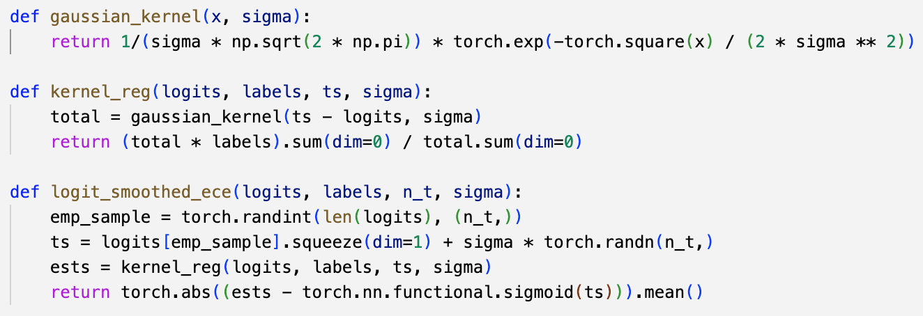
Figure 1: Implementation of $\mathrm{LS}\text{-}\mathrm{ECE}_{\hat{\pi},\xi}(h)$ in 10 lines of PyTorch (Paszke et al., 2019) using broadcast semantics.

We need only now prove that $\mathrm{LS}\text{-}\mathrm{ECE}_{\hat{\pi},\xi}(h)$ converges in probability to $\mathrm{LS}\text{-}\mathrm{ECE}_{\pi,\xi}(h)$, i.e. that estimating $\mathrm{LS}\text{-}\mathrm{ECE}_{\hat{\pi},\xi}$ allows us to consistently estimate $\mathrm{LS}\text{-}\mathrm{ECE}_{\pi,\xi}(h)$. We note that here $\mathrm{LS}\text{-}\mathrm{ECE}_{\pi,\xi}(h)$ is a non-random scalar quantity depending on the logit function $h$ while $\mathrm{LS}\text{-}\mathrm{ECE}_{\hat{\pi},\xi}(h)$ is a random variable depending on the pairs $(x_{i},y_{i})\sim\pi$.

It turns out that the only additional stipulation on $\xi$ necessary to achieve consistency is that $\xi$ be of the form $\xi=\sigma R$ for a random variable $R$ with bounded density (for example, $\xi\sim\mathcal{N}(0,\sigma^{2})$). So long as $\xi$ is of this type, we can prove that $p_{\hat{T}}\to p_{T}$ and $p_{\hat{T},Y=1}\to p_{T,Y=1}$ in $L^{1}$, which is all we need for consistency. This is encapsulated in the following lemma, which once again may be of independent interest.

Lemma 5.2.

If $\xi=\sigma R$ for a random variable $R$ with bounded density, then:

$$\mathbb{E}_{\pi}\left[\int_{0}^{1}\absolutevalue{p_{T,Y=1}(t)-p_{\hat{T},Y=1}(t)}\ dt\right] =O\left(\frac{1}{\sqrt{n\sigma}}\right),$$ (5.7)

$$\mathbb{E}_{\pi}\left[\int_{0}^{1}\absolutevalue{p_{T}(t)-p_{\hat{T}}(t)}\ dt\right] =O\left(\frac{1}{\sqrt{n\sigma}}\right).$$ (5.8)

Proof of Lemma 5.2.

We recall that $p_{T,Y=1}(t)$ has the following form, which is a result of Proposition 5.1:

$$p_{T,Y=1}(t)=(\rho^{-1})^{\prime}(t)\,\pi_{Y}(1)\,\mathbb{E}\left[p_{\xi}(\rho^{-1}(t)-h(X))\mid Y=1\right].$$ (5.9)

Now from Cauchy–Schwarz, Jensen’s inequality, Fubini’s theorem, and a change of variable (in that order), we obtain:

$$\mathbb{E}_{\pi}\bigg{[}\int_{0}^{1}\absolutevalue{p_{T,Y=1}(t)-p_{\hat{T},Y=1}(t)}\ dt\bigg{]} \leq\mathbb{E}_{\pi}\left[\sqrt{\int_{0}^{1}\absolutevalue{p_{T,Y=1}(t)-p_{\hat{T},Y=1}(t)}^{2}\ dt}\right]$$

$$\leq\sqrt{\int_{0}^{1}\mathbb{E}_{\pi}\left[\absolutevalue{p_{T,Y=1}(t)-p_{\hat{T},Y=1}(t)}^{2}\right]\ dt}$$

$$=\Bigg{(}\int_{0}^{1}\mathbb{E}_{\pi}\bigg{[}\bigg{|}(\rho^{-1})^{\prime}(t)\,\pi_{Y}(1)\,\mathbb{E}\left[p_{\xi}(\rho^{-1}(t)-h(X))\mid Y=1\right]$$

$$\quad\quad\quad-\frac{1}{n}\sum_{i=1}^{n}(\rho^{-1})^{\prime}(t)\,p_{\xi}(\rho^{-1}(t)-h(x_{i}))\,\mathbbm{1}_{y_{i}=1}\bigg{|}^{2}\bigg{]}\ dt\Bigg{)}^{1/2}$$

$$=\Bigg{(}\int_{-\infty}^{\infty}\mathbb{E}_{\pi}\bigg{[}\bigg{|}\pi_{Y}(1)\,\mathbb{E}\left[p_{\xi}(u-h(X))\mid Y=1\right]$$

$$\quad\quad\quad-\frac{1}{n}\sum_{i=1}^{n}p_{\xi}(u-h(x_{i}))\,\mathbbm{1}_{y_{i}=1}\bigg{|}^{2}\bigg{]}\ du\Bigg{)}^{1/2}.$$ (5.10)

For simplicity, let us make the following definitions before moving forward:

$$f(u) =\pi_{Y}(1)\,\mathbb{E}\left[p_{\xi}(u-h(X))\mid Y=1\right],$$ (5.11)

$$\hat{f}(u) =\frac{1}{n}\sum_{i=1}^{n}p_{\xi}(u-h(x_{i}))\,\mathbbm{1}_{y_{i}=1}.$$ (5.12)

We observe that $\mathbb{E}_{\pi}[\hat{f}(u)]=f(u)$ for every $u$, since the $(x_{i},y_{i})$ are i.i.d. according to $\pi$. Now we can continue from (5.10):

$$\mathbb{E}_{\pi}\bigg{[}\int_{0}^{1}\absolutevalue{p_{T,Y=1}(t)-p_{\hat{T},Y=1}(t)}\ dt\bigg{]} \leq\sqrt{\int_{-\infty}^{\infty}\mathbb{E}_{\pi}\left[\absolutevalue{f(u)-\hat{f}(u)}^{2}\right]\ du}$$

$$=\sqrt{\int_{-\infty}^{\infty}\mathrm{Var}_{\pi}(\hat{f}(u))\ du}$$

$$\leq\sqrt{\frac{\pi_{Y}(1)^{2}}{n}\int_{-\infty}^{\infty}\mathbb{E}\left[p_{\xi}(u-h(X))^{2}\mid Y=1\right]\ du}$$

$$=\sqrt{\frac{\pi_{Y}(1)^{2}}{n\sigma}\mathbb{E}\left[\int_{-\infty}^{\infty}\frac{M}{\sigma}p_{R}\left(\frac{u-h(X)}{\sigma}\right)\ du\mid Y=1\right]}$$

$$=O\left(\frac{1}{\sqrt{n\sigma}}\right)$$ (5.13)

where $M=\sup p_{R}$. The result for $\absolutevalue{p_{T}(t)-p_{\hat{T}}(t)}$ follows identically. ∎

With Lemma 5.2, we prove our main estimation result.

Theorem 5.3.

If $\xi=\sigma R$ for a random variable $R$ with bounded density, we have that

$$\mathbb{E}_{\pi}\big{[}\absolutevalue{\mathrm{LS}\text{-}\mathrm{ECE}_{\pi,\xi}(h)-\mathrm{LS}\text{-}\mathrm{ECE}_{\hat{\pi},\xi}(h)}\big{]}=O\big{(}1/\sqrt{n\sigma}\big{)},$$ (5.14)

which implies $\mathrm{LS}\text{-}\mathrm{ECE}_{\hat{\pi},\xi}(h)\to\mathrm{LS}\text{-}\mathrm{ECE}_{\pi,\xi}(h)$ in probability.

Proof.

Let $T$ be as in Lemma 5.2, i.e. the population form of $\hat{T}$. Then we have by the triangle inequality:

$$\mathbb{E}_{\pi}\big{[}\absolutevalue{\mathrm{LS}\text{-}\mathrm{ECE}_{\pi,\xi}(h)-\mathrm{LS}\text{-}\mathrm{ECE}_{\hat{\pi},\xi}(h)}\big{]}$$

$$=\mathbb{E}_{\pi}\Bigg{[}\bigg{|}\int_{0}^{1}\absolutevalue{\mathbb{E}[Y\mid T=t]-t}p_{T}(t)\ dt-\int_{0}^{1}\absolutevalue{\mathbb{E}[Y\mid\hat{T}=t]-t}p_{\hat{T}}(t)\ dt\bigg{|}\Bigg{]}$$

$$\leq\mathbb{E}_{\pi}\bigg{[}\int_{0}^{1}\absolutevalue{p_{T,Y=1}(t)-p_{\hat{T},Y=1}(t)}\ dt+\int_{0}^{1}t\absolutevalue{p_{T}(t)-p_{\hat{T}}(t)}\ dt\bigg{]}.$$ (5.15)

Noting that $t\leq 1$ and applying Lemma 5.2 shows that the final line of (5.15) is $O(1/\sqrt{n\sigma})$, which is the desired result. ∎

The quantitative bound in Theorem 5.3 shows that choosing $\sigma$ in practice is — as intuition would suggest from the discussion of kernel regression — similar to choosing the kernel bandwidth. In general, $\sigma$ can be thought of as a hyperparameter, but we will see in Section 6 that experiments are relatively insensitive to the choice of $\sigma$.

5.1 Consequences for Estimation of ECE

Nevertheless, for theoretical purposes, the scaling of $\sigma$ is important. The bound in Theorem 5.3 suggests that $\sigma$ should be at least $\omega(1/n)$ to prevent the estimation error from exploding.

It is then natural to ask what happens if we take $\sigma=\omega(1/n)$ but $\sigma\to 0$ as $n\to\infty$. By doing so — analogously, once again, to existing results in the kernel density estimation literature — we obtain that $\mathrm{LS}\text{-}\mathrm{ECE}_{\hat{\pi},\xi_{n}}(h)$ actually becomes a consistent estimator of the true ECE, under appropriate conditions on the logit distribution $h(X)$. This is a non-trivial estimation result that we effectively get for free as a result of our framework, as shown in the short proof below.

Theorem 5.4.

Suppose $\xi=\sigma R$ for a random variable $R$ with bounded, almost everywhere continuous density, and let $\xi_{n}=\sigma_{n}\xi$ with $\sigma_{n}$ satisfying $\lim_{n\to\infty}\sigma_{n}=0$ and $\sigma_{n}=\omega(1/n)$. If the conditional distribution of $h(X)$ conditioned on $Y=y$ has an almost everywhere continuous density for $y\in\{0,1\}$, then $\mathrm{LS}\text{-}\mathrm{ECE}_{\hat{\pi},\xi_{n}}(h)\to\mathrm{ECE}_{\pi}(\rho\circ h)$ in probability.

Proof.

First we claim that if $Z$ has an a.e. continuous density $p_{Z}$, then $Z+\xi_{n}\to Z$ in total variation. This follows by noting that $p_{\sigma\xi}(x)=\frac{1}{\sigma}p_{\xi}\left(\frac{x}{\sigma}\right)$ is a sequence of good kernels (i.e. an approximation to the identity) (Stein & Shakarchi, 2011), so that

$$p_{Z+\xi_{n}}(x)=(p_{Z}*p_{\xi_{n}})(x)\to p_{Z}(x)$$

at any continuity point of $p_{Z}$. Then $Z+\xi_{n}\stackrel{{\scriptstyle\mathrm{TV}}}{{\to}}Z$ by Scheffé’s Lemma.

Now for $y\in\{0,1\}$, by assumption and the above claim, conditioned on $Y=y$, $h(X)+\xi_{n}\stackrel{{\scriptstyle\mathrm{TV}}}{{\to}}h(X)$. Hence $(Y,h(X)+\xi_{n})\stackrel{{\scriptstyle\mathrm{TV}}}{{\to}}(Y,h(X))$.

By Lemma 4.4, $|\mathrm{LS}\text{-}\mathrm{ECE}_{\pi,\xi_{n}}(h)-\mathrm{ECE}_{\pi}(\rho\circ h)|\to 0$ as $n\to\infty$. The result then follows from the triangle inequality and Theorem 5.3. ∎

Comparison to existing estimation results. To our knowledge, the only existing consistency results for ECE (or, more specifically, the $L^{1}$ ECE) are the works of Zhang et al. (2020) and Popordanoska et al. (2022) that show consistency via adapting corresponding results for kernel density estimation. These results thus require assumptions such as Hölder-smooth and bounded or Lipschitz continuity of the density of $h(X)$ conditioned on $Y=y$, whereas we require only a.e. continuity.

6 Experiments

We now empirically verify that $\mathrm{LS}\text{-}\mathrm{ECE}_{\pi,\xi}$ behaves nicely even when $\mathrm{ECE}_{\pi}$ does not. We revisit the simple 2-point data distribution of Definition 3.1 in Section 6.1, and show that the discontinuity at $g(x)=1/2$ leads to oscillatory behavior in $\mathrm{ECE}_{\mathrm{BIN},\pi}$ (defined above in (2.3)) as we change the number of bins, whereas $\mathrm{LS}\text{-}\mathrm{ECE}_{\hat{\pi},\xi}$ remains effectively constant irrespective of the choice of variance for $\xi$. On the other hand, we also show that for image classification using a wide range of models, $\mathrm{ECE}_{\mathrm{BIN},\pi}$ changes smoothly as we vary the number of bins, and the resulting estimates match up closely with $\mathrm{LS}\text{-}\mathrm{ECE}_{\hat{\pi},\xi}$.

6.1 Synthetic Data

We consider data drawn from a distribution $\pi$ as in Definition 3.1, and the predictor $g(x)=\rho(\alpha x)$ where $\rho$ is the sigmoid function and $\alpha=10^{-3}$. We construct $g$ in this way so that $g(-0.5)=1/2-\epsilon$ and $g(0.5)=1/2+\epsilon$, i.e. $g$ matches our discussion in Section 3.1.

As we already know, $\mathrm{ECE}_{\pi}$ is discontinuous at the predictor which always predicts $1/2$. This immediately presents a problem for the estimation of $\mathrm{ECE}_{\pi}(g)$ via $\mathrm{ECE}_{\mathrm{BIN},\pi}(g)$; indeed, one can readily compute (as done in (Błasiok et al., 2023)) that $\mathrm{ECE}_{\mathrm{BIN},\pi}(g)$ jumps between $\approx 0$ and $\approx 1/2$ depending on the parity of the number of bins used. We visualize this behavior in Figure 2, where we plot $\mathrm{ECE}_{\mathrm{BIN},\pi}(g)$ evaluated on 1000 samples from $\pi$ with the number of bins ranging from $1$ to $100$.

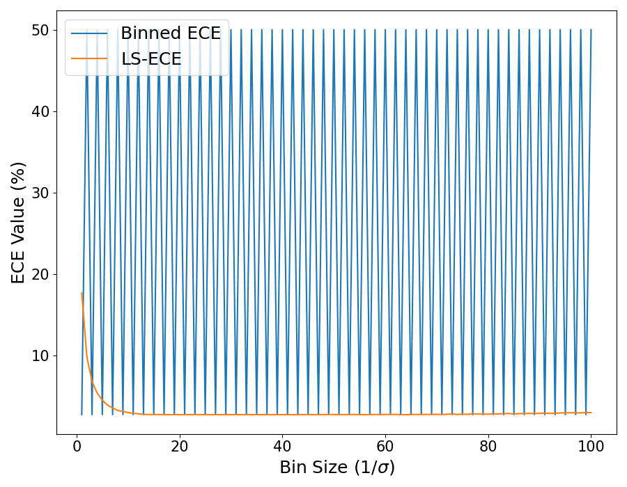
Figure 2: Comparison of $\mathrm{ECE}_{\mathrm{BIN},\pi}$ (blue) and $\mathrm{LS}\text{-}\mathrm{ECE}_{\pi,\xi}$ (orange) over bins (and correspondingly, inverse scalings for $\xi$) ranging from 1 to 100 on the model and data setup of Section 6.1.

Alongside $\mathrm{ECE}_{\mathrm{BIN},\pi}(g)$, we also plot $\mathrm{LS}\text{-}\mathrm{ECE}_{\hat{\pi},\xi}(h)$, where $h(x)=\alpha x$ and $\xi\sim\mathcal{N}(0,\sigma^{2})$. We let $\sigma$ be the inverse of the number of bins used for $\mathrm{ECE}_{\mathrm{BIN},\pi}(g)$. The motivation for this choice of $\sigma$ comes from considering a uniform kernel (i.e. $\xi\sim\sigma\mathrm{Uni}([-1/2,1/2])$), since in this case $\sigma$ corresponds to the bin size centered at each point. We estimate $\mathrm{LS}\text{-}\mathrm{ECE}_{\hat{\pi},\xi}(h)$ via 10000 independent samples drawn from the distribution of $h(X)+\xi$, as discussed in Section 5. We see that, outside the case of large $\sigma$ (i.e. $\sigma\gtrsim 1$), $\mathrm{LS}\text{-}\mathrm{ECE}_{\hat{\pi},\xi}(h)$ remains effectively constant near zero and entirely avoids the oscillatory behavior of $\mathrm{ECE}_{\mathrm{BIN},\pi}$.

6.2 Image Classification

More importantly, we now check whether this disparity between $\mathrm{ECE}_{\mathrm{BIN},\pi}(g)$ and $\mathrm{LS}\text{-}\mathrm{ECE}_{\hat{\pi},\xi}(h)$ appears in settings of practical interest. We consider CIFAR-10, CIFAR-100 (Krizhevsky, 2009), and ImageNet (Deng et al., 2009) and compare $\mathrm{ECE}_{\mathrm{BIN},\pi}(g)$ using the bin numbers $\{1,10,20,...,100\}$ to $\mathrm{LS}\text{-}\mathrm{ECE}_{\hat{\pi},\xi}(h)$ with inversely proportional $\sigma$ and $\xi\sim\mathcal{N}(0,\sigma^{2})$. As before, we estimate $\mathrm{LS}\text{-}\mathrm{ECE}_{\hat{\pi},\xi}(h)$ using 10000 independent samples drawn from the distribution of $h(X)+\xi$.

Since all of the experiments in this section deal with multi-class classification, we use the top-class formulations of ECE and LS-ECE (see (2.2)). For LS-ECE, we construct the logit function $h(x)$ as $h(x)=\rho^{-1}(\max_{i}g^{i}(x))$, i.e. we apply the inverse sigmoid function to the maximum predicted probability.

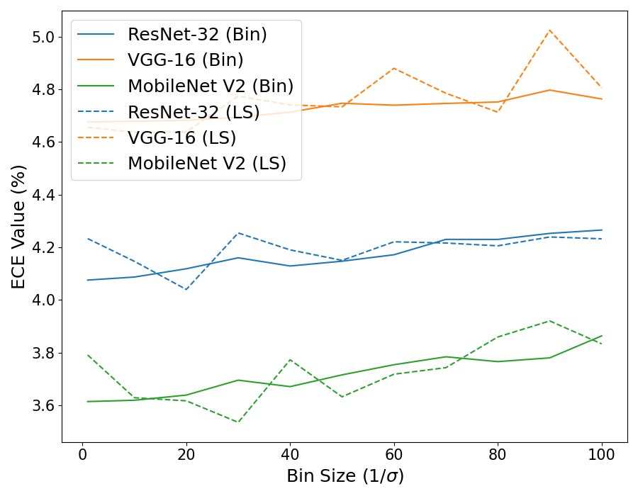
(a) CIFAR-10

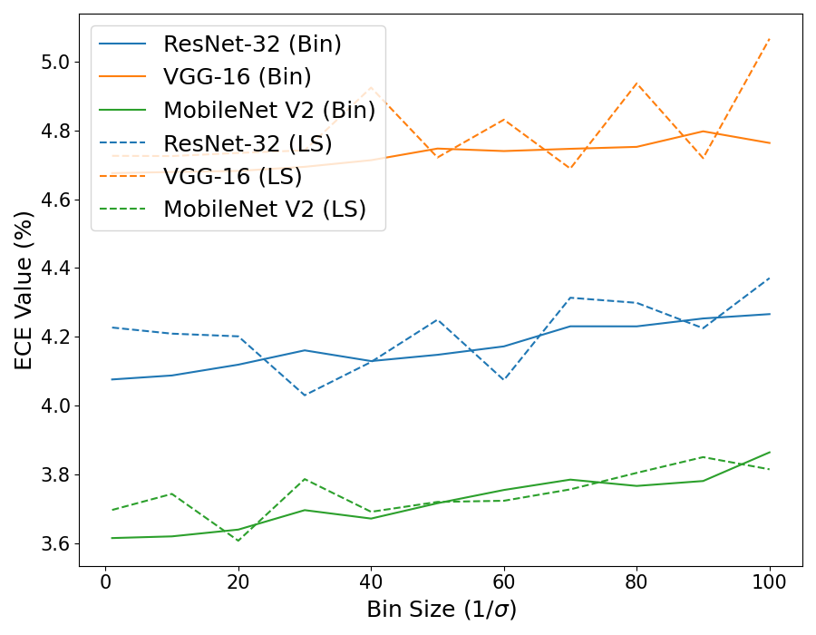
(b) CIFAR-100

Figure 3: Comparison of $\mathrm{ECE}_{\mathrm{BIN},\pi}$ and $\mathrm{LS}\text{-}\mathrm{ECE}_{\pi,\xi}$ for different models on CIFAR datasets over bins/variance scalings ranging from 1 to 100. Solid lines correspond to $\mathrm{ECE}_{\mathrm{BIN},\pi}$ and dashed lines correspond to $\mathrm{LS}\text{-}\mathrm{ECE}_{\pi,\xi}$.

6.2.1 CIFAR Experiments

For our CIFAR experiments, we use pretrained versions (due to Yaofo Chen) of ResNet-32 (He et al., 2015), VGG-16 (Simonyan & Zisserman, 2015), and MobileNetV2 (Sandler et al., 2019) available on TorchHub. Results for evaluating these models on the CIFAR-10 and CIFAR-100 test data are shown in Figure 3.

As can be seen, $\mathrm{ECE}_{\mathrm{BIN},\pi}(g)$ stays nearly the same as we change the number of bins, and $\mathrm{LS}\text{-}\mathrm{ECE}_{\pi,\xi}(h)$ tracks it quite closely. (Although $\mathrm{LS}\text{-}\mathrm{ECE}_{\pi,\xi}(h)$ visually appears to exhibit more variance, the scale of this variance is small.) Furthermore, we note that the conclusions drawn from both ECE and LS-ECE about which model is best calibrated stay consistent across the choice of bin number/variance scaling.

6.2.2 ImageNet Experiments

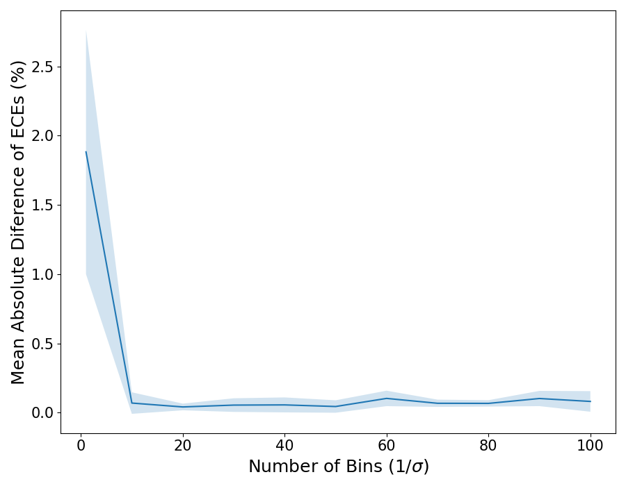
Figure 4: Mean absolute difference between ECE and LS-ECE on ImageNet-1K-val over all models considered in Section 6.2.2, with one standard deviation error bounds marked using the shaded region.

We repeat our CIFAR experimental setup for ImageNet, and consider a gamut of pretrained architectures: ResNet-18 and ResNet-50 (He et al., 2015; Wightman et al., 2021), EfficientNet (Tan & Le, 2019), MobileNetV3 (Howard et al., 2019), Vision Transformer (Dosovitskiy et al., 2021), RegNet (Radosavovic et al., 2020), and ConvNeXt (Liu et al., 2022). All of our models are obtained from the timm (Wightman, 2019) library and were pretrained using the techniques described by Wightman et al. (2021). We evaluate all models on the ImageNet-1K validation data, and in Figure 4 we report the mean absolute difference (over all models) between ECE and LS-ECE, across bin numbers and choices of $\sigma$ respectively, with one-standard-deviation error bounds.

The ImageNet results further corroborate our CIFAR findings: ECE and LS-ECE take near-identical values for all models considered, across the range of possible bin numbers and variances. Although this is by no means a comprehensive evaluation, the fact that the continuous LS-ECE so closely tracks ECE in these experiments suggests that the theoretical pathologies of ECE may not pose a problem for assessing the calibration of real-world models in practice.

7 Conclusion

In summary, we have entirely characterized the discontinuities of ECE in a very general setting. We further used these continuity results to motivate the construction of LS-ECE, a continuous analogue of ECE that tracks it closely, and which in fact can be used to obtain a consistent estimator of ECE. As the results in this work are largely theoretical, a natural direction for future work would be a large-scale empirical validation of ECE results in the literature using the ideas we have presented.

References

- Arrieta-Ibarra et al. (2022) Arrieta-Ibarra, I., Gujral, P., Tannen, J., Tygert, M., and Xu, C. Metrics of calibration for probabilistic predictions. arXiv preprint arXiv:2205.09680, 2022.
- Bröcker (2008) Bröcker, J. Some remarks on the reliability of categorical probability forecasts. Monthly weather review, 136(11):4488–4502, 2008.
- Brown et al. (2020) Brown, T., Mann, B., Ryder, N., Subbiah, M., Kaplan, J. D., Dhariwal, P., Neelakantan, A., Shyam, P., Sastry, G., Askell, A., Agarwal, S., Herbert-Voss, A., Krueger, G., Henighan, T., Child, R., Ramesh, A., Ziegler, D., Wu, J., Winter, C., …, and Amodei, D. Language models are few-shot learners. In Advances in Neural Information Processing Systems, volume 33, pp. 1877–1901. Curran Associates, Inc., 2020. URL https://proceedings.neurips.cc/paper/2020/file/1457c0d6bfcb4967418bfb8ac142f64a-Paper.pdf.
- Błasiok & Nakkiran (2023) Błasiok, J. and Nakkiran, P. Smooth ece: Principled reliability diagrams via kernel smoothing, 2023.
- Błasiok et al. (2023) Błasiok, J., Gopalan, P., Hu, L., and Nakkiran, P. A unifying theory of distance from calibration, 2023.
- Dawid (1982) Dawid, A. P. The well-calibrated bayesian. Journal of the American Statistical Association, 77(379):605–610, 1982.
- DeGroot & Fienberg (1983) DeGroot, M. H. and Fienberg, S. E. The comparison and evaluation of forecasters. Journal of the Royal Statistical Society: Series D (The Statistician), 32(1-2):12–22, 1983.
- Deng et al. (2009) Deng, J., Dong, W., Socher, R., Li, L.-J., Li, K., and Fei-Fei, L. Imagenet: A large-scale hierarchical image database. In 2009 IEEE Conference on Computer Vision and Pattern Recognition, pp. 248–255, 2009. doi: 10.1109/CVPR.2009.5206848.
- Dimitriadis et al. (2021) Dimitriadis, T., Gneiting, T., and Jordan, A. I. Stable reliability diagrams for probabilistic classifiers. Proceedings of the National Academy of Sciences, 118(8):e2016191118, 2021.
- Dosovitskiy et al. (2021) Dosovitskiy, A., Beyer, L., Kolesnikov, A., Weissenborn, D., Zhai, X., Unterthiner, T., Dehghani, M., Minderer, M., Heigold, G., Gelly, S., Uszkoreit, J., and Houlsby, N. An image is worth 16x16 words: Transformers for image recognition at scale. ICLR, 2021.
- Elmarakeby et al. (2021) Elmarakeby, H. A., Hwang, J., Arafeh, R., Crowdis, J., Gang, S., Liu, D., AlDubayan, S. H., Salari, K., Kregel, S., Richter, C., et al. Biologically informed deep neural network for prostate cancer discovery. Nature, 598(7880):348–352, 2021.
- Foster & Hart (2018) Foster, D. P. and Hart, S. Smooth calibration, leaky forecasts, finite recall, and nash dynamics. Games Econ. Behav., 109:271–293, 2018. URL https://doi.org/10.1016/j.geb.2017.12.022.
- Guo et al. (2017) Guo, C., Pleiss, G., Sun, Y., and Weinberger, K. Q. On calibration of modern neural networks. In International Conference on Machine Learning, pp. 1321–1330. PMLR, 2017.
- Gupta et al. (2021) Gupta, K., Rahimi, A., Ajanthan, T., Mensink, T., Sminchisescu, C., and Hartley, R. Calibration of neural networks using splines. In International Conference on Learning Representations, 2021.
- He et al. (2015) He, K., Zhang, X., Ren, S., and Sun, J. Deep residual learning for image recognition. CoRR, abs/1512.03385, 2015. URL http://arxiv.org/abs/1512.03385.
- Howard et al. (2019) Howard, A., Sandler, M., Chu, G., Chen, L.-C., Chen, B., Tan, M., Wang, W., Zhu, Y., Pang, R., Vasudevan, V., et al. Searching for mobilenetv3. In Proceedings of the IEEE/CVF international conference on computer vision, pp. 1314–1324, 2019.
- Hu et al. (2023) Hu, Y., Yang, J., Chen, L., Li, K., Sima, C., Zhu, X., Chai, S., Du, S., Lin, T., Wang, W., Lu, L., Jia, X., Liu, Q., Dai, J., Qiao, Y., and Li, H. Planning-oriented autonomous driving, 2023.
- Kakade & Foster (2008) Kakade, S. and Foster, D. Deterministic calibration and nash equilibrium. Journal of Computer and System Sciences, 74(1):115–130, 2008.
- Krizhevsky (2009) Krizhevsky, A. Learning multiple layers of features from tiny images. pp. 32–33, 2009. URL https://www.cs.toronto.edu/~kriz/learning-features-2009-TR.pdf.
- Kudô (1974) Kudô, H. A note on the strong convergence of -algebras. Annals of Probability, 2:76–83, 1974.
- Kumar et al. (2018) Kumar, A., Sarawagi, S., and Jain, U. Trainable calibration measures for neural networks from kernel mean embeddings. In International Conference on Machine Learning, pp. 2805–2814. PMLR, 2018.
- Kumar et al. (2019) Kumar, A., Liang, P. S., and Ma, T. Verified uncertainty calibration. In Advances in Neural Information Processing Systems, pp. 3792–3803, 2019.
- Lakshminarayanan et al. (2017) Lakshminarayanan, B., Pritzel, A., and Blundell, C. Simple and scalable predictive uncertainty estimation using deep ensembles. In Advances in neural information processing systems, pp. 6402–6413, 2017.
- Lee et al. (2022) Lee, D., Huang, X., Hassani, H., and Dobriban, E. T-cal: An optimal test for the calibration of predictive models. arXiv preprint arXiv:2203.01850, 2022.
- Liu et al. (2022) Liu, Z., Mao, H., Wu, C.-Y., Feichtenhofer, C., Darrell, T., and Xie, S. A convnet for the 2020s. Proceedings of the IEEE/CVF Conference on Computer Vision and Pattern Recognition (CVPR), 2022.
- Minderer et al. (2021) Minderer, M., Djolonga, J., Romijnders, R., Hubis, F., Zhai, X., Houlsby, N., Tran, D., and Lucic, M. Revisiting the calibration of modern neural networks. Advances in Neural Information Processing Systems, 34:15682–15694, 2021.
- Müller et al. (2020) Müller, R., Kornblith, S., and Hinton, G. When does label smoothing help?, 2020.
- Nadaraya (1964) Nadaraya, E. A. On estimating regression. Theory of Probability & Its Applications, 9(1):141–142, 1964. doi: 10.1137/1109020. URL https://doi.org/10.1137/1109020.
- Naeini et al. (2014) Naeini, M. P., Cooper, G. F., and Hauskrecht, M. Binary classifier calibration: Non-parametric approach. arXiv preprint arXiv:1401.3390, 2014.
- Nixon et al. (2019) Nixon, J., Dusenberry, M. W., Zhang, L., Jerfel, G., and Tran, D. Measuring calibration in deep learning. In CVPR Workshops, volume 2, 2019.
- Nogales et al. (2021) Nogales, A., Álvaro J. García-Tejedor, Monge, D., Vara, J. S., and Antón, C. A survey of deep learning models in medical therapeutic areas. Artificial Intelligence in Medicine, 112:102020, 2021. ISSN 0933-3657. doi: https://doi.org/10.1016/j.artmed.2021.102020. URL https://www.sciencedirect.com/science/article/pii/S0933365721000130.
- OpenAI (2023) OpenAI. Gpt-4 technical report, 2023.
- Paszke et al. (2019) Paszke, A., Gross, S., Massa, F., Lerer, A., Bradbury, J., Chanan, G., Killeen, T., Lin, Z., Gimelshein, N., Antiga, L., Desmaison, A., Köpf, A., Yang, E. Z., DeVito, Z., Raison, M., Tejani, A., Chilamkurthy, S., Steiner, B., Fang, L., Bai, J., and Chintala, S. Pytorch: An imperative style, high-performance deep learning library. CoRR, abs/1912.01703, 2019. URL http://arxiv.org/abs/1912.01703.
- Popordanoska et al. (2022) Popordanoska, T., Sayer, R., and Blaschko, M. A consistent and differentiable lp canonical calibration error estimator. Advances in Neural Information Processing Systems, 35:7933–7946, 2022.
- Radosavovic et al. (2020) Radosavovic, I., Kosaraju, R. P., Girshick, R., He, K., and Doll’ar, P. Designing network design spaces. In CVPR, 2020.
- Ramesh et al. (2022) Ramesh, A., Dhariwal, P., Nichol, A., Chu, C., and Chen, M. Hierarchical text-conditional image generation with clip latents, 2022. URL https://arxiv.org/abs/2204.06125.
- Roelofs et al. (2022) Roelofs, R., Cain, N., Shlens, J., and Mozer, M. C. Mitigating bias in calibration error estimation. In International Conference on Artificial Intelligence and Statistics, pp. 4036–4054. PMLR, 2022.
- Sandler et al. (2019) Sandler, M., Howard, A., Zhu, M., Zhmoginov, A., and Chen, L.-C. Mobilenetv2: Inverted residuals and linear bottlenecks, 2019.
- Simonyan & Zisserman (2015) Simonyan, K. and Zisserman, A. Very deep convolutional networks for large-scale image recognition, 2015.
- Stein & Shakarchi (2011) Stein, E. M. and Shakarchi, R. Fourier analysis: an introduction, volume 1. Princeton University Press, 2011.
- Tan & Le (2019) Tan, M. and Le, Q. Efficientnet: Rethinking model scaling for convolutional neural networks. In International conference on machine learning, pp. 6105–6114. PMLR, 2019.
- Thulasidasan et al. (2019) Thulasidasan, S., Chennupati, G., Bilmes, J. A., Bhattacharya, T., and Michalak, S. On mixup training: Improved calibration and predictive uncertainty for deep neural networks. Advances in Neural Information Processing Systems, 32:13888–13899, 2019.
- Touvron et al. (2023) Touvron, H., Lavril, T., Izacard, G., Martinet, X., Lachaux, M.-A., Lacroix, T., Rozière, B., Goyal, N., Hambro, E., Azhar, F., Rodriguez, A., Joulin, A., Grave, E., and Lample, G. Llama: Open and efficient foundation language models, 2023.
- Vaicenavicius et al. (2019) Vaicenavicius, J., Widmann, D., Andersson, C., Lindsten, F., Roll, J., and Schön, T. Evaluating model calibration in classification. In The 22nd International Conference on Artificial Intelligence and Statistics, pp. 3459–3467. PMLR, 2019.
- Wang & Golebiowski (2023) Wang, C. and Golebiowski, J. Meta-calibration regularized neural networks, 2023.
- Wang et al. (2021) Wang, D.-B., Feng, L., and Zhang, M.-L. Rethinking calibration of deep neural networks: Do not be afraid of overconfidence. In Ranzato, M., Beygelzimer, A., Dauphin, Y., Liang, P., and Vaughan, J. W. (eds.), Advances in Neural Information Processing Systems, volume 34, pp. 11809–11820. Curran Associates, Inc., 2021. URL https://proceedings.neurips.cc/paper_files/paper/2021/file/61f3a6dbc9120ea78ef75544826c814e-Paper.pdf.
- Watson (1964) Watson, G. S. Smooth regression analysis. Sankhyā: The Indian Journal of Statistics, Series A (1961-2002), 26(4):359–372, 1964. ISSN 0581572X. URL http://www.jstor.org/stable/25049340.
- Wightman (2019) Wightman, R. Pytorch image models. https://github.com/rwightman/pytorch-image-models, 2019.
- Wightman et al. (2021) Wightman, R., Touvron, H., and Jégou, H. Resnet strikes back: An improved training procedure in timm. CoRR, abs/2110.00476, 2021. URL https://arxiv.org/abs/2110.00476.
- Zhang et al. (2020) Zhang, J., Kailkhura, B., and Han, T. Y.-J. Mix-n-match: Ensemble and compositional methods for uncertainty calibration in deep learning. In International conference on machine learning, pp. 11117–11128. PMLR, 2020.