How to validate average calibration for machine learning regression tasks ?

Abstract

Average calibration of the uncertainties of machine learning regression tasks can be tested in two ways. One way is to estimate the calibration error (CE) as the difference between the mean absolute error (MSE) and the mean variance (MV) or mean squared uncertainty. The alternative is to compare the mean squared z-scores or scaled errors (ZMS) to 1. Both approaches might lead to different conclusion, as illustrated on an ensemble of datasets from the recent machine learning uncertainty quantification literature. It is shown here that the CE is very sensitive to the distribution of uncertainties, and notably to the presence of outlying uncertainties, and that it cannot be used reliably for average calibration testing. By contrast, the ZMS statistic does not present this sensitivity issue and offers the most reliable approach in this context. Implications for the validation of conditional calibration are discussed.

I Introduction

The assessment of prediction uncertainty calibration for machine learning (ML) regression tasks is based on two main statistics: (1) the calibration errors (CE: UCE, ENCE(Levi2022, )…) which are based on the comparison of the mean squared errors (MSE) to mean squared uncertainties or mean variance (MV); and (2) the Negative Log-Likelihood (NLL(Gneiting2007b, ; Tran2020, ; Rasmussen2023, )) which is based on the mean of squared z-scores or scaled errors (ZMS(Pernot2023d, )).

Average calibration has been shown to be insufficient to guarantee the reliability of uncertainties across data space(Kuleshov2018, ), but it remains a necessary condition that is too often overlooked in calibration studies.

The MSE = MV equation has been used to test or establish average calibration(Wellendorff2014, ; Pernot2017, ), but it mostly occurs in ML through a bin-based setup, meaning that it measures conditional calibration. As the binning variable is generally the uncertainty(Levi2022, ; Frenkel2023, ), the UCE and ENCE are typically used to measure consistency, as defined by Pernot(Pernot2023d, ). In post hoc calibration, scaling factors for the uncertainties can be derived from the ZMS ($\sigma$ scaling(Laves2020, ), BVS(Frenkel2023, ; Pernot2023c_arXiv, )) or from the UCE(Frenkel2023, ).

This short study focuses on the comparison of CE- and ZMS-based approaches to validate average calibration. The interest of these average calibration statistics is to have a predefined reference value, enabling direct statistical testing. This is not the case for bin-based statistics such as the UCE and ENCE, for which validation is much more complex(Pernot2023a_arXiv, ). De facto, the latter are practically used only in comparative studies, without validation.

The next section defines the calibration statistics and the validation approach. Sect. III illustrates the comparison of these statistics over an ensemble of datasets issued from the ML-UQ literature and proposes an analysis of the results. The main conclusions are reported in Sect. IV.

II Average calibration statistics

Let us consider a dataset composed of paired errors and uncertainties $\left\{E_{i},u_{E_{i}}\right\}_{i=1}^{M}$ to be tested for average calibration. The variance-based UQ validation statistics are built on a probabilistic model linking errors to uncertainties

$$E_{i}\sim u_{E_{i}}D(0,1)$$ (1)

where $D(\mu,\sigma)$ is an unspecified probability density function with mean $\mu$ and standard deviation $\sigma$. This model states that errors are expected to be unbiased ($\mu=0$) and that uncertainty quantifies the dispersion of errors, according to the metrological definition(GUM, ).

II.1 The calibration error and related statistics

Let us assume that the errors are drawn from a distribution $D(0,\sigma)$ with unknown scale parameter $\sigma$, itself distributed according to a distribution $G$. The distribution of errors is then a scale mixture distribution $H$, with probability density function

$$p_{H}(E)={\displaystyle\int_{0}^{\infty}p_{D}(E|\sigma)\,p_{G}(\sigma)\thinspace d\sigma}$$ (2)

and the variance of the compound distribution of errors is obtained by the law of total variance

$$\mathrm{Var}(E) =\left\langle\mathrm{Var}_{D}(E|\sigma)\right\rangle_{G}+\mathrm{Var}_{G}\left(\left\langle E|\sigma\right\rangle_{D}\right)$$ (3)

$$=<u_{E}^{2}>+\mathrm{Var}_{G}\left(\left\langle E|\sigma\right\rangle_{D}\right)$$ (4)

The first term of the RHS is the mean squared uncertainty $<u_{E}^{2}>$. This expression can be compared to the standard expression for the variance

$$\mathrm{Var}(E) =<E^{2}>-<E>^{2}$$ (5)

For an unbiased error distribution, one gets $\mathrm{Var}_{G}\left(\left\langle E|\sigma\right\rangle_{D}\right)=0$ and $<E>=0$, leading to

$$<E^{2}>=<u_{E}^{2}>$$ (6)

Based on this equation, the Relative Calibration Error is aimed to test average calibration, and is defined as

$$RCE=\frac{RMV-RMSE}{RMV}$$ (7)

where $RMSE$ is the root mean squared error $\sqrt{<E^{2}>}$ and $RMV$ is the root mean variance ($\sqrt{<u_{E}^{2}>}$). The RCE statistic does not depend on the shape of $D$ and its reference value is 0.

The RCE occurs in a bin-based statistic of conditional calibration,(Pernot2023d, ) the Expected Normalized Calibration Error(Levi2022, )

$$ENCE=\frac{1}{N}\sum_{i=1}^{N}|RCE_{i}|$$ (8)

where $RCE_{i}$ is estimated over the data in bin $i$. Depending on the variable chosen to design the bins, the ENCE might be used to test consistency (binning on $u_{E}$) or adaptivity (binning on input features).(Pernot2023d, ) The ENCE has no predefined reference value (it depends on the dataset and the binning scheme)(Pernot2023a_arXiv, ), which complicates its use for statistical testing of conditional calibration.

II.2 $ZMS$ and related statistics

Another approach to calibration based on Eq. 1 uses scaled errors or z-scores

$$Z_{i}=\frac{E_{i}}{u_{E_{i}}}\sim D(0,1)$$ (9)

with the property

$$Var(Z)=1$$ (10)

assessing average calibration for unbiased errors(Pernot2022a, ; Pernot2022b, ). If one accepts that the uncertainties have been tailored to cover biased errors, the calibration equation becomes

$$ZMS=<Z^{2}>=1$$ (11)

which is the preferred form for testing(Pernot2023d, ), notably when a dataset is split into subsets for the assessment of conditional calibration. The ZMS does not depend on the shape of $D$ and its target value is 1. Note that for homoscedastic datasets ($u_{E}=const.)$, one gets $RCE=1-ZMS$.

The negative log-likelihood (NLL) score for a normal likelihood is linked to the ZMS by(Busk2023, )

$$NLL =\frac{1}{2}\left(<Z^{2}>+<\ln u_{E}^{2}>+\ln 2\pi\right)$$ (12)

It combines the ZMS as an average calibration term(Zhang2023, ) to a sharpness term driving the uncertainties towards small values(Gneiting2007a, ) when the NLL is used as a loss function, hence preventing the minimization of $<Z^{2}>$ by arbitrary large uncertainties. For a given set of uncertainties, testing the NLL value is equivalent to testing the ZMS value.

II.3 Validation

For a given dataset $(E,u_{E})$ and a statistic $\vartheta$, one estimates the statistic over the dataset $\vartheta_{est}$, and a bootstrapped sample from which one gets the bias of the bootstrapped distribution $b_{BS}$ and a 95 % confidence interval $I_{BS}=\left[I_{BS}^{-},I_{BS}^{+}\right]$. Note that it is generally not recommended to correct $\vartheta_{est}$ from the bootstrapping bias $b_{BS}$, but it is important to check that the bias is negligible. Considering that errors and uncertainties have generally non-normal distributions, and that it is not reliable to invoke the Central Limit Theorem to use normality-based testing approaches (see Pernot(Pernot2022a, )), one has to infer confidence intervals on the statistics by bootstrapping (BS). The most reliable approach in these conditions is considered to be the Bias Corrected Accelerated (BC_a) method(DiCiccio1996, ), which is used throughout this study.

The most straightforward validation approach is then to check that the target value for the statistic, $\vartheta_{ref}$, lies within $I_{BS}$, i.e.

$$\vartheta_{ref}\in\left[I_{BS}^{-},I_{BS}^{+}\right]$$ (13)

To go beyond this binary result, it is interesting to have a continuous measure of agreement, and one can define a standardized score $\zeta$ as the ratio of the signed distance of the estimated value $\vartheta_{est}$ to its reference $\vartheta_{ref}$, over the absolute value of the distance between the $\vartheta_{est}$ and the limit of the confidence interval closest to $\vartheta_{ref}$. More concretely

$$\zeta(\vartheta_{est},\vartheta_{ref},I_{BS})=\begin{cases}\frac{\vartheta_{est}-\vartheta_{ref}}{I_{BS}^{+}-\vartheta_{est}}&if\,(\vartheta_{est}-\vartheta_{ref})\leq 0\\ \frac{\vartheta_{est}-\vartheta_{ref}}{\vartheta_{est}-I_{BS}^{-}}&if\,(\vartheta_{est}-\vartheta_{ref})>0\end{cases}$$ (14)

which considers explicitly the possible asymmetry of $I_{BS}$ around $\vartheta_{est}$. The compatibility of the statistic with its reference value can then be tested by

$$|\zeta|\leq 1$$ (15)

which is strictly equivalent to the interval test (Eq. 13). In addition to testing, $\zeta$ provides valuable information about the sign and amplitude of the mismatch between the statistic and its reference value.

III Experiments

The validation approach presented above is applied to nine datasets extracted from the ML-UQ literature, and the results are analyzed.

III.1 The datasets

Nine test sets, including errors and calibrated uncertainties, have been taken from the recent ML-UQ literature for the prediction of various physico-chemical properties by a diverse panel of ML methods. This selection rejected small datasets and those presenting duplicated properties. Note that for all the datasets, the uncertainties have been calibrated by a palette of methods with various levels of success. The datasets names, sizes and bibliographic references are gathered in Table 1, and the reader is referred to the original articles for further details. In the following, a short notation is used, e.g. ’Set 7’ corresponds to the QM9_E dataset.

Set #	Name	$M$	$\beta_{GM}(u_{E})$			Reference
1	Diffusion_RF	2040	0.	172		Palmer et al.(Palmer2022, )
2	Perovskite_RF	3834	0.	419		Palmer et al.(Palmer2022, )
3	Diffusion_LR	2040	0.	485		Palmer et al.(Palmer2022, )
4	Perovskite_LR	3836	0.	438		Palmer et al.(Palmer2022, )
5	Diffusion_GPR_Bayesian	2040	0.	113		Palmer et al.(Palmer2022, )
6	Perovskite_GPR_Bayesian	3818	-			Palmer et al.(Palmer2022, )
7	QM9_E	13885	0.	524		Busk et al.(Busk2022, )
8	logP_10k_a_LS-GCN	5000	0.	231		Rasmussen et al.(Rasmussen2023, )
9	logP_150k_LS-GCN	5000	0.	223		Rasmussen et al.(Rasmussen2023, )

Table 1: The nine datasets used in this study: number, name, size, skewness of uncertainties and reference.

As the shape of the uncertainty distribution plays a major role in the coming analysis, the uncertainty distributions were characterized by $\beta_{GM}$, a skewness statistic based on the scaled difference between the mean and median (Groeneveld1984, ; Pernot2021, ). $\beta_{GM}$ is robust to outliers, varies between -1 and 1 and is null for symmetric distributions. The values reported in Table 1 vary between 0.172 and 0.524. $\beta_{GM}$ is not reported for Set 6, as it has a strongly bimodal uncertainty distribution for which skewness is not a pertinent descriptor.

III.2 Comparison of validation results

The statistics and confidence intervals have been estimated for the RCE and ZMS for all datasets with $10^{4}$ bootstrap replicates. The reference values $\vartheta_{ref}$ are 0 for the RCE and 1 for the ZMS. The results are reported in Table 2. It is clear from these results that average calibration is satisfied by all datasets and, more problematically, that the diagnostic depends on the choice of statistic.

Set	RCE		bias		95 % CI	$\zeta_{RCE}$
1	0.	01860	6.	1e-04	[-0.0209, 0.0542]	0.	47
2	-0.	03870	5.	2e-04	[-0.107, 0.0193]	-0.	67
3	-0.	00748	-8.	2e-06	[-0.0524, 0.04]	-0.	16
4	0.	05450	-1.	2e-03	[0.000718, 0.126]	1.	01
5	0.	09860	4.	9e-04	[0.0574, 0.135]	2.	39
6	0.	09240	1.	2e-03	[0.00335, 0.16]	1.	04
7	-0.	26400	8.	6e-03	[-0.685, -0.0028]	-1.	01
8	0.	04590	1.	3e-04	[0.00676, 0.0777]	1.	17
9	-0.	01310	1.	2e-04	[-0.0715, 0.0263]	-0.	33

Set	ZMS	bias	95 % CI	$\zeta_{ZMS}$
1	0.960	-1.0e-03	[0.867, 1.1]	-0.28
2	0.885	-1.8e-05	[0.803, 0.995]	-1.05
3	1.120	-1.5e-04	[1.05, 1.2]	1.67
4	1.230	1.3e-04	[1.16, 1.3]	3.48
5	0.846	-6.3e-04	[0.777, 0.929]	-1.85
6	0.984	-2.0e-04	[0.857, 1.15]	-0.10
7	0.972	-1.9e-04	[0.936, 1.01]	-0.71
8	0.926	3.7e-05	[0.869, 0.993]	-1.10
9	0.971	1.7e-04	[0.901, 1.08]	-0.27

Table 2: RCE and ZMS statistics and their validation results. The bold characters signal sets where $|\zeta|\leq 1$.

Comparison of the absolute $\zeta$-scores for ZMS and RCE across the nine datasets shows a contrasted situation (Fig. 1):

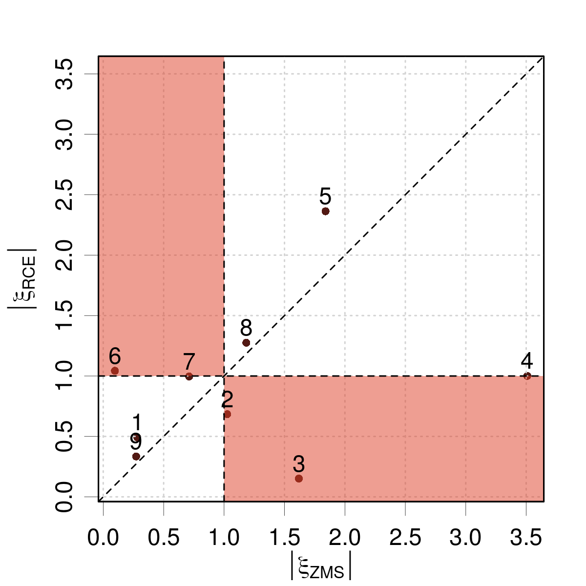
Figure 1: Comparison of the absolute $\zeta$-scores for ZMS and RCE. The symbols represent the set numbers in Table 2. The colored areas contain the disagreeing validation results.

• points close to the identity line and more globally in uncolored areas, are the datasets for which both statistics agree on the calibration diagnostic, i.e. positive for Sets 1and 9, and negative for Set 5 and 8.

• two sets have ambiguous validation results for RCE, as they lie on top or are very close to the validation limit (Sets 4 and 7). For Set 4 the RCE and ZMS values are very different, which is less marked for Set 7.

• Set 6 is validated by the ZMS and rejected by the RCE and both scores are very different,

• finally, Sets 2 and 3 are validated by RCE and rejected by ZMS.

It is remarkable that four of the five sets for which a disagreement between RCE and ZMS is observed (Sets 2, 3, 4 and 7) are those with the largest skewness values (Table 1), suggesting that the right tail of the uncertainty distribution plays a major role in this phenomenon. Set 6 cannot be reliably described by a skewness factor and its case will be elucidated below.

Globally, the statistics disagree on more than half of the datasets, which is somewhat surprising for two statistics deriving analytically from the same generative model (Eq. 1).

III.3 Analysis

In order to understand the discrepancy of the validation results by RCE and ZMS, one needs to consider the sensitivity of these statistics to the uncertainty distributions, and notably to the large, sometimes outlying, values, as suggested by the skewness analysis. In the z-scores, these values are likely to contribute to small absolute values of $Z$ having a small impact on the ZMS, while they are likely to affect significantly the estimation of the RMV. This hypothesis is tested on the nine datasets by a decimating experiment, where both statistics are evaluated on datasets iteratively pruned from their largest uncertainties, and by a simulation experiment with synthetic uncertainty sets of varying skewness.

III.3.1 Sensitivity to the upper tail of the uncertainty distributions

The deviations of the ZMS and RCE scores from their value for the full dataset are estimated for an iterative pruning of the datasets from their largest uncertainties, as performed in confidence curves(Pernot2022c, ). The values of $\Delta_{RCE}=RCE_{k}-RCE_{0}$ and $\Delta_{ZMS}=ZMS_{k}-ZMS_{0}$ for a percentage $k$ of discarded data varying between 0 and 10 % are shown in Fig. 2, where zero-centered bootstrapped 95 %CIs for both statistics are displayed as vertical bars to help to assess the amplitude of the deviations.

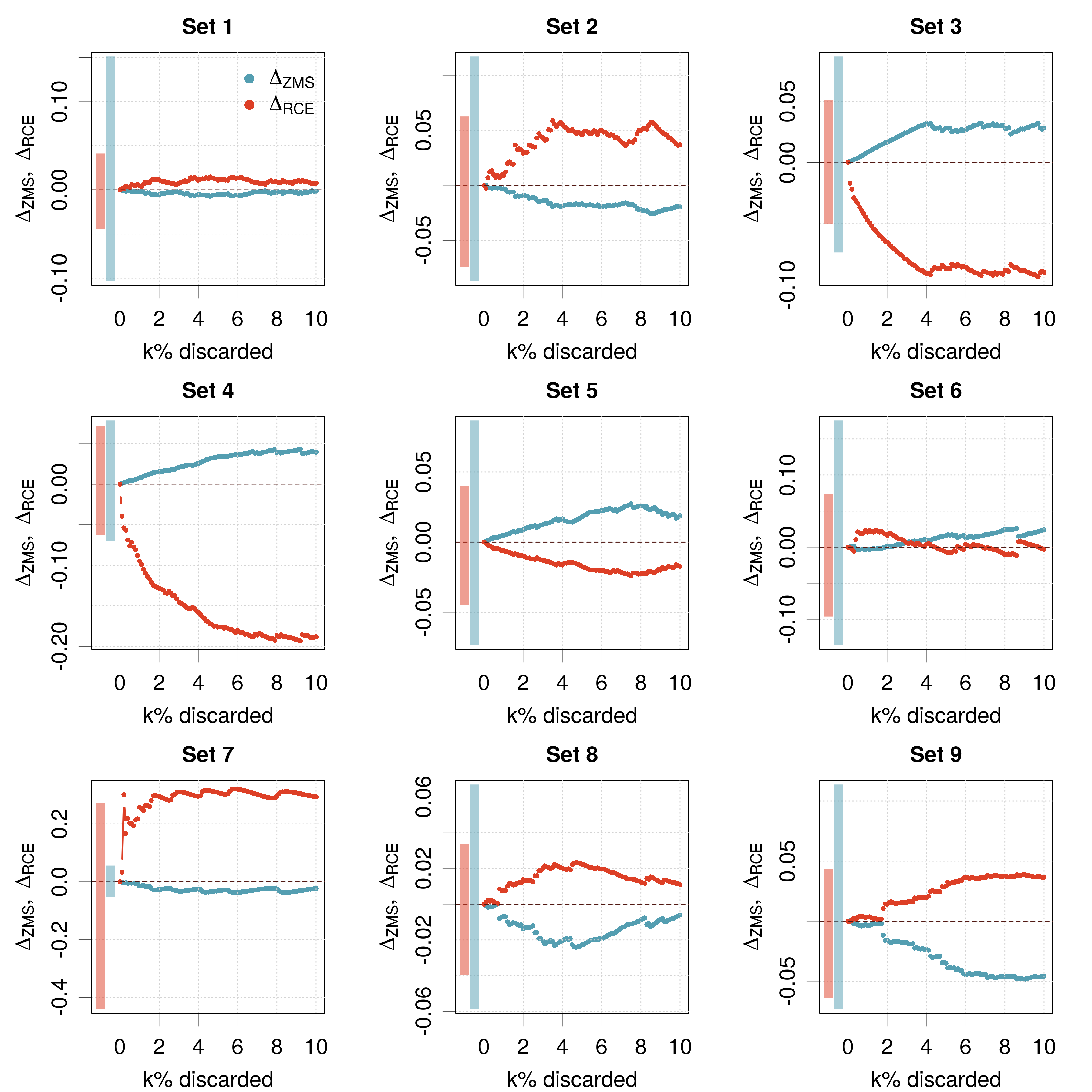
Figure 2: Variation of the RCE and ZMS statistics according to the percentage $k$ of largest uncertainties removed from the datasets. The vertical colored bars represent 95 % confidence intervals on the statistics for the full datasets.

It appears that in all cases the ZMS is less or as sensitive as the RCE and that its curve always strays within the limits of the corresponding CI. For the RCE, one can find cases where the RCE is more sensitive than the ZMS but lies within the limits of the CI (Sets 2 and 6) and cases where it strays beyond the limits of the CI (Sets 3, 4 and 7). The five latter cases are precisely those where the RCE diagnostic differs the most from the ZMS.

This sensitivity test by dataset decimation confirms the hypothesis that the RCE is more sensitive than the ZMS to the upper tail of the uncertainty distribution, to a point where its estimation might become unreliable.

III.3.2 Reliability for skewed uncertainty distributions

To characterize the impact of the sensitivity of the RCE and ZMS statistics to the upper tail of the uncertainty distribution in a validation context, a comparison of the rates of failure of validation tests for both statistics is also performed on synthetic datasets: $N_{MC}=10^{3}$ synthetic datasets of size $M=5000$ are generated using Eq. 1 with a normal generative distribution [$D=N(0,1)$] and Inverse Gamma distributions for $u_{E}^{2}$ [$u_{E}^{2}\sim IG(\nu/2,\nu/2)$], with degrees of freedom ($\nu$) varying between 2 and 20. The skewness of the $IG$ distribution decreases as $\nu$ increases, but is not defined for $\nu\leq 6$. This combination of probability density functions generates errors with a Student’s-t distribution with $\nu$ degrees of freedom ($E\sim t(\nu)$). $t(2)$ is a distribution with infinite variance, and it is assumed that $t(20)$ is close to a normal distribution. This is a sub-case of the NIG distribution used in evidential inference.(Amini2019, )

For each sample, the calibration was tested using $|\zeta|\leq 1$ and a probability of validity was estimated as

$$p_{val}=\frac{1}{N}\sum_{i=1}^{N}\boldsymbol{1}(|\zeta|_{i}\leq 1)$$ (16)

where $\boldsymbol{1}(x)$ is the indicator function with values 0 when $x$ is false, and 1 when $x$ is true. The values of $p_{val}$ with their 95% CIs obtained by a binomial model(Pernot2022a, ), are plotted in Fig. 3 for the RCE and ZMS statistics as a function of $\nu$. The upper axis provides the average $\beta_{GM}$ statistic for the generated $IG$ samples.

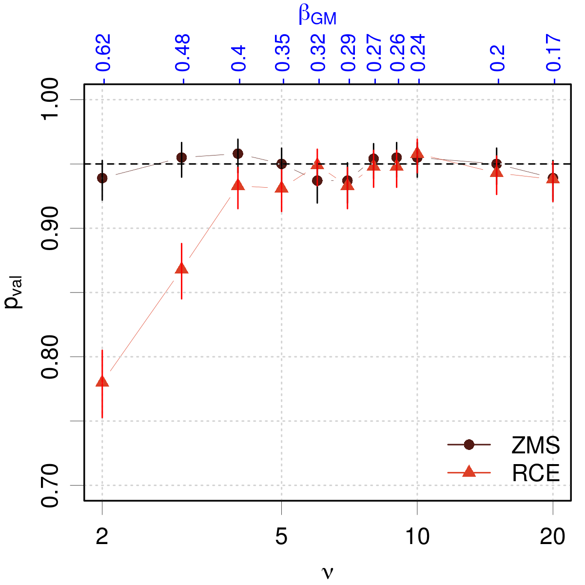
Figure 3: Validation probability of the ZMS and RCE statistics for calibrated datasets generated from the NIG model with $\nu$ degrees of freedom.

This test shows that the ZMS is not sensitive to $\nu$, even for extreme uncertainty distributions, and that it provides intervals that consistently validate 95 % of the calibrated synthetic datasets. For the RCE, the validation error is strongly sensitive to $\nu$ for values below 4, reaching more than 20 % for $\nu=2$. In terms of $\beta_{GM}$ the safety limit for the RCE seems to be below 0.4. These observations confirm the conclusions obtained on the literature datasets.

IV Conclusion

This study focused on the reliability of RCE and ZMS as average calibration statistics. Discrepancies of diagnostic between both statistics was observed for an ensemble of nine datasets extracted from the recent ML-UQ literature for regression tasks. This anomaly has been elucidated by showing that the RCE is much more sensitive than the ZMS to the upper tail of the uncertainty distribution, and notably to the presence of outliers. A consequence is that average calibration statistics based on the comparison of $MSE=<E^{2}>$ to $MV=<u_{E}^{2}>$ should not be relied upon for the kind of datasets found in ML-UQ regression problems. In contrast, the ZMS statistic, which deals globally with the better-behaved distributions of scaled errors ($Z=E/u_{E}$) has no reliability issue and should therefore be the statistic of choice for average calibration testing.

This finding has consequences for the validation of conditional calibration. The popular UCE and ENCE statistics implement the comparison of MV to MSE statistics, but, being bin-based, they are less susceptible to be affected by this sensitivity issue when the binning variable is $u_{E}$ (consistency testing(Pernot2023d, )). For a large enough number of bins, the problem of large outlying $u_{E}$ values should vanish, or at least be confined to a single bin. Unfortunately, this is not the case if the UCE or ENCE are based on another binning variable (such as an input feature), as is requested to test adaptivity.(Pernot2023d, ) In this case, each bin might contain a large range of uncertainty values, leading to the reliability problem. It might therefore be better to assess conditional calibration by binned ZMS statistics.

Author Declarations

Conflict of Interest

The author has no conflicts to disclose.

Code and data availability

The code and data to reproduce the results of this article are available at https://github.com/ppernot/2024_RCE/releases/tag/v1.0 and at Zenodo (https://doi.org/10.5281/zenodo.10666788).

References

- (1) D. Levi, L. Gispan, N. Giladi, and E. Fetaya. Evaluating and Calibrating Uncertainty Prediction in Regression Tasks. Sensors, 22:5540, 2022.
- (2) T. Gneiting and A. E. Raftery. Strictly Proper Scoring Rules, Prediction, and Estimation. J. Am. Stat. Assoc., pages 359–378, 2007.
- (3) K. Tran, W. Neiswanger, J. Yoon, Q. Zhang, E. Xing, and Z. W. Ulissi. Methods for comparing uncertainty quantifications for material property predictions. Mach. Learn.: Sci. Technol., 1:025006, 2020.
- (4) M. H. Rasmussen, C. Duan, H. J. Kulik, and J. H. Jensen. Uncertain of uncertainties? A comparison of uncertainty quantification metrics for chemical data sets. J. Cheminf., 15:1–17, December 2023.
- (5) P. Pernot. Calibration in machine learning uncertainty quantification: Beyond consistency to target adaptivity. APL Mach. Learn., 1:046121, 2023.
- (6) V. Kuleshov, N. Fenner, and S. Ermon. Accurate uncertainties for deep learning using calibrated regression. In J. Dy and A. Krause, editors, Proceedings of the 35th International Conference on Machine Learning, volume 80 of Proceedings of Machine Learning Research, pages 2796–2804. PMLR, 10–15 Jul 2018. URL: https://proceedings.mlr.press/v80/kuleshov18a.html.
- (7) J. Wellendorff, K. T. Lundgaard, K. W. Jacobsen, and T. Bligaard. mBEEF: An accurate semi-local bayesian error estimation density functional. J. Chem. Phys., 140:144107, 2014.
- (8) P. Pernot and F. Cailliez. A critical review of statistical calibration/prediction models handling data inconsistency and model inadequacy. AIChE J., 63:4642–4665, 2017.
- (9) L. Frenkel and J. Goldberger. Calibration of a regression network based on the predictive variance with applications to medical images. In 2023 IEEE 20th International Symposium on Biomedical Imaging (ISBI), pages 1–5. IEEE, 2023.
- (10) M.-H. Laves, S. Ihler, J. F. Fast, L. A. Kahrs, and T. Ortmaier. Well-calibrated regression uncertainty in medical imaging with deep learning. In T. Arbel, I. Ben Ayed, M. de Bruijne, M. Descoteaux, H. Lombaert, and C. Pal, editors, Proceedings of the Third Conference on Medical Imaging with Deep Learning, volume 121 of Proceedings of Machine Learning Research, pages 393–412. PMLR, 06–08 Jul 2020. URL: https://proceedings.mlr.press/v121/laves20a.html.
- (11) P. Pernot. Can bin-wise scaling improve consistency and adaptivity of prediction uncertainty for machine learning regression ? arXiv:2310.11978, October 2023.
- (12) P. Pernot. Properties of the ENCE and other MAD-based calibration metrics. arXiv:2305.11905, May 2023.
- (13) BIPM, IEC, IFCC, ILAC, ISO, IUPAC, IUPAP, and OIML. Evaluation of measurement data - Guide to the expression of uncertainty in measurement (GUM). Technical Report 100:2008, Joint Committee for Guides in Metrology, JCGM, 2008. URL: http://www.bipm.org/utils/common/documents/jcgm/JCGM_100_2008_F.pdf.
- (14) P. Pernot. The long road to calibrated prediction uncertainty in computational chemistry. J. Chem. Phys., 156:114109, 2022.
- (15) P. Pernot. Prediction uncertainty validation for computational chemists. J. Chem. Phys., 157:144103, 2022.
- (16) J. Busk, M. N. Schmidt, O. Winther, T. Vegge, and P. B. Jørgensen. Graph neural network interatomic potential ensembles with calibrated aleatoric and epistemic uncertainty on energy and forces. Phys. Chem. Chem. Phys., 25:25828–25837, 2023.
- (17) W. Zhang, Z. Ma, S. Das, T.-W. Weng, A. Megretski, L. Daniel, and L. M. Nguyen. One step closer to unbiased aleatoric uncertainty estimation. arXiv:2312.10469, December 2023.
- (18) T. Gneiting, F. Balabdaoui, and A. E. Raftery. Probabilistic forecasts, calibration and sharpness. J. R. Statist. Soc. B, 69:243–268, 2007.
- (19) T. J. DiCiccio and B. Efron. Bootstrap confidence intervals. Statist. Sci., 11:189–212, 1996. URL: https://www.jstor.org/stable/2246110.
- (20) G. Palmer, S. Du, A. Politowicz, J. P. Emory, X. Yang, A. Gautam, G. Gupta, Z. Li, R. Jacobs, and D. Morgan. Calibration after bootstrap for accurate uncertainty quantification in regression models. npj Comput. Mater., 8:115, 2022.
- (21) J. Busk, P. B. Jørgensen, A. Bhowmik, M. N. Schmidt, O. Winther, and T. Vegge. Calibrated uncertainty for molecular property prediction using ensembles of message passing neural networks. Mach. Learn.: Sci. Technol., 3:015012, 2022.
- (22) R. A. Groeneveld and G. Meeden. Measuring skewness and kurtosis. The Statistician, 33:391–399, 1984. URL: http://www.jstor.org/stable/2987742.
- (23) P. Pernot and A. Savin. Using the Gini coefficient to characterize the shape of computational chemistry error distributions. Theor. Chem. Acc., 140:24, 2021.
- (24) P. Pernot. Confidence curves for UQ validation: probabilistic reference vs. oracle. arXiv:2206.15272, June 2022.
- (25) A. Amini, W. Schwarting, A. Soleimany, and D. Rus. Deep Evidential Regression. arXiv:1910.02600, October 2019.