Diffusion Models Meet Contextual Bandits with Large Action Spaces

Abstract

Efficient exploration is a key challenge in contextual bandits due to the large size of their action space, where uninformed exploration can result in computational and statistical inefficiencies. Fortunately, the rewards of actions are often correlated and this can be leveraged to explore them efficiently. In this work, we capture such correlations using pre-trained diffusion models; upon which we design diffusion Thompson sampling (dTS). Both theoretical and algorithmic foundations are developed for dTS, and empirical evaluation also shows its favorable performance.

1 Introduction

A contextual bandit is a popular and practical framework for online learning under uncertainty (Li et al., 2010). In each round, an agent observes a context, takes an action, and receives a reward based on the context and action. The goal is to maximize the expected cumulative reward over $n$ rounds, striking a balance between exploiting actions with high estimated rewards from available data and exploring other actions to improve current estimates. This trade-off is often addressed using either upper confidence bound (UCB) (Auer et al., 2002) or Thompson sampling (TS) (Scott, 2010).

The action space in contextual bandits is often large, resulting in less-than-optimal performance with standard exploration strategies. Luckily, actions often exhibit correlations, making efficient exploration possible as one action may inform the agent about other actions. In particular, Thompson sampling offers remarkable flexibility, allowing its integration with informative prior distributions (Hong et al., 2022b) that can capture these correlations. Inspired by the achievements of diffusion models (Sohl-Dickstein et al., 2015; Ho et al., 2020), which effectively approximate complex distributions (Dhariwal & Nichol, 2021; Rombach et al., 2022), this work captures action correlations by employing diffusion models as priors in contextual Thompson sampling.

We illustrate the idea using a video streaming scenario. The objective is to optimize watch time for a user $j$ by selecting a video $i$ from a catalog of $K$ videos. Users $j$ and videos $i$ are associated with context vectors $x_{j}$ and unknown video parameters $\theta_{i}$, respectively. User $j$’s expected watch time for video $i$ is linear as $x_{j}^{\top}\theta_{i}$. Then, a natural strategy would be to independently learn video parameters $\theta_{i}$ using LinTS or LinUCB (Agrawal & Goyal, 2013a; Abbasi-Yadkori et al., 2011), but this proves statistically inefficient for larger $K$. Luckily, videos exhibit correlations and can provide informative insights into one another. To capture this, we leverage offline estimates of video parameters denoted by $\hat{\theta}_{i}$ and build a diffusion model on them. This diffusion model approximates the video parameter distribution, capturing their dependencies. This model enriches contextual Thompson sampling as a prior, effectively capturing complex video dependencies while ensuring computational efficiency.

Formally, we present a unified contextual bandit framework represented by diffusion models. On this basis, we design a computationally and statistically efficient diffusion Thompson sampling (dTS). We then specialize dTS on linear instances, for which we provide closed-form solutions and establish an upper bound for its Bayes regret. The regret bound reflects the structure of the problem and the quality of the priors, demonstrating the benefits of using diffusion models as priors (dTS) over the standard methods. Beyond enabling theoretical analysis, these linear instances motivate an efficient approximation for general non-linear ones. Finally, our empirical evaluations validate our theory and demonstrate the strong performance of dTS with closed-form solutions as well as dTS with approximations.

Diffusion models have been used for offline decision-making (Ajay et al., 2022; Janner et al., 2022; Wang et al., 2022). However, their use in online learning was only recently explored by Hsieh et al. (2023), who focused on multi-armed bandits without theoretical guarantees. Our work extends Hsieh et al. (2023) in two ways. First, we extend the idea to the broader contextual bandit framework. This allows us to consider problems where the rewards depend on the context, which is more realistic. Second, we show that when the diffusion model is parametrized by linear score functions, we can derive recursive closed-form posteriors without the need for approximations. Closed-form posteriors are particularly interesting because they facilitate theoretical analysis and motivate more computationally efficient approximations for the case with non-linear score functions; making dTS more scalable. Finally, we provide a theoretical analysis of dTS, which effectively captures the benefits of employing linear diffusion models as priors within contextual Thompson sampling. An extended comparison to related works is provided in Appendix A, where we discuss the broader topics of diffusion models and decision-making, hierarchical, structured and low-rank bandits, approximate posteriors, etc.

2 Setting

The agent interacts with a contextual bandit over $n$ rounds. In round $t\in[n]$, the agent observes a context $X_{t}\in\mathcal{X}$, where $\mathcal{X}\subseteq\mathbb{R}^{d}$ is a $d$-dimensional context space, it takes an action $A_{t}\in[K]$, and then receives a stochastic reward $Y_{t}\in\mathbb{R}$ that depends on both the context $X_{t}$ and the taken action $A_{t}$. Each action $i\in[K]$ is associated with an unknown action parameter $\theta_{*,i}\in^{d}$, so that the reward received in round $t$ is $Y_{t}\sim P(\cdot\mid X_{t};\theta_{*,A_{t}})$, where $P(\cdot\mid x;\theta_{*,a})$ is the reward distribution of action $a$ in context $x$. We consider the Bayesian bandit setting (Russo & Van Roy, 2014; Hong et al., 2022b), where the action parameters $\theta_{*,i}$ are assumed to be sampled from a known prior distribution. We proceed to define this prior distribution using a diffusion model.

The correlations between the action parameters $\theta_{*,i}$ are captured through a diffusion model, where they share a set of $L$ consecutive unknown latent parameters $\psi_{*,\ell}$ for $\ell\in[L]$. Precisely, the action parameter $\theta_{*,i}$ depends on the $L$-th latent parameter $\psi_{*,L}$ as $\theta_{*,i}\mid\psi_{*,1}\sim\mathcal{N}(f_{1}(\psi_{*,1}),\Sigma_{1})$, where the score function $f_{1}:^{d}\rightarrow^{d}$ is known. Also, the $\ell-1$-th latent parameter $\psi_{*,\ell-1}$ depends on the $\ell$-th latent parameter $\psi_{*,\ell}$ as $\psi_{*,\ell-1}\mid\psi_{*,\ell}\sim\mathcal{N}(f_{\ell}(\psi_{*,\ell}),\Sigma_{\ell})$, where the score function $f_{\ell}:^{d}\rightarrow^{d}$ is known. Finally, the $L$-th latent parameter $\psi_{*,L}$ is sampled as $\psi_{*,L}\sim\mathcal{N}(0,\Sigma_{L+1})$. We summarize this model in (1) and its graph in Figure 1.

$$\psi_{*,L} \sim\mathcal{N}(0,\Sigma_{L+1})\,,$$ (1)

$$\psi_{*,\ell-1}\mid\psi_{*,\ell} \sim\mathcal{N}(f_{\ell}(\psi_{*,\ell}),\Sigma_{\ell})\,, \forall\ell\in[L]/\{1\}\,,$$

$$\theta_{*,i}\mid\psi_{*,1} \sim\mathcal{N}(f_{1}(\psi_{*,1}),\Sigma_{1})\,, \forall i\in[K]\,,$$

$$Y_{t}\mid X_{t},\theta_{*,A_{t}} \sim P(\cdot\mid X_{t};\theta_{*,A_{t}})\,, \forall t\in[n]\,.$$

The model in (1) represents a Bayesian bandit. The agent interacts with a bandit instance defined by the action parameters $\theta_{*,i}$ over $n$ rounds (4-th line in (1)). These action parameters $\theta_{*,i}$ are drawn from the generative process in the first 3 lines of (1). Note that (1) can be built by pre-training a diffusion model on offline estimates of the action parameters $\theta_{*,i}$ (Hsieh et al., 2023).

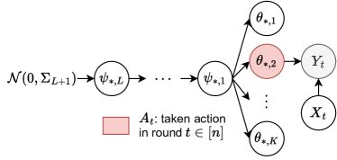
Figure 1: Graphical model induced by (1).

A natural goal for the agent in this Bayesian framework is to minimize its Bayes regret (Russo & Van Roy, 2014) that measures the expected performance across multiple bandit instances $\theta_{*}=(\theta_{*,i})_{i\in[K]}$,

$$\mathcal{B}\mathcal{R}(n)=\mathbb{E}\left[\sum_{t=1}^{n}r(X_{t},A_{t,*};\theta_{*})-r(X_{t},A_{t};\theta_{*})\right]\,,$$ (2)

where the expectation in (2) is taken over all random variables in (1). Here $r(x,i;\theta_{*})=\mathbb{E}_{Y\sim P(\cdot\mid x;\theta_{*,i})}\left[Y\right]$ is the expected reward of action $i$ in context $x$ and $A_{t,*}=\operatorname*{arg\,max}_{i\in[K]}r(X_{t},i;\theta_{*})$ is the optimal action in round $t$. The Bayes regret is known to capture the benefits of using informative priors, and hence it is suitable for our problem.

3 Algorithm

We design Thompson sampling that samples the latent and action parameters hierarchically (Lindley & Smith, 1972). Precisely, let $H_{t}=(X_{k},A_{k},Y_{k})_{k\in[t-1]}$ be the history of all interactions up to round $t$ and let $H_{t,i}=(X_{k},A_{k},Y_{k})_{\{k\in[t-1];A_{k}=i\}}$ be the history of interactions with action $i$ up to round $t$. To motivate our algorithm, we decompose the posterior $\mathbb{P}\left(\theta_{*,i}=\theta\,\middle|\,H_{t}\right)$ recursively as

$$\textstyle\mathbb{P}\left(\theta_{*,i}=\theta\,\middle|\,H_{t}\right)= \textstyle\int_{\psi_{1:L}}Q_{t,L}(\psi_{L})\prod_{\ell=2}^{L}Q_{t,\ell-1}(\psi_{\ell-1}\mid\psi_{\ell})$$

$$\textstyle\qquad\,\,P_{t,i}(\theta\mid\psi_{1})\mathop{}\!\mathrm{d}\psi_{1:L}\,,\quad\text{where}$$ (3)

$Q_{t,L}(\psi_{L})=\mathbb{P}\left(\psi_{*,L}=\psi_{L}\,\middle|\,H_{t}\right)$ is the latent-posterior density of $\psi_{*,L}\mid H_{t}$. Moreover, for any $\ell\in[L]/\{1\}$, $Q_{t,\ell-1}(\psi_{\ell-1}\mid\psi_{\ell})=\mathbb{P}\left(\psi_{*,\ell-1}=\psi_{\ell-1}\,\middle|\,H_{t},\psi_{*,\ell}=\psi_{\ell}\right)$ is the conditional latent-posterior density of $\psi_{*,\ell-1}\mid H_{t},\psi_{*,\ell}=\psi_{\ell}$. Finally, for any action $i\in[K]$, $P_{t,i}(\theta\mid\psi_{1})=\mathbb{P}\left(\theta_{*,i}=\theta\,\middle|\,H_{t,i},\psi_{*,1}=\psi_{1}\right)$ is the conditional action-posterior density of $\theta_{*,i}\mid H_{t,i},\psi_{*,1}=\psi_{1}$.

The decomposition in (3) inspires hierarchical sampling. In round $t$, we initially sample the $L$-th latent parameter as $\psi_{t,L}\sim Q_{t,L}(\cdot)$. Then, for $\ell\in[L]/\{1\}$, we sample the $\ell-1$-th latent parameter given that $\psi_{*,\ell}=\psi_{t,\ell}$, as $\psi_{t,\ell-1}\sim Q_{t,\ell-1}(\cdot\mid\psi_{t,\ell})$. Lastly, given that $\psi_{*,1}=\psi_{t,1}$, each action parameter is sampled individually as $\theta_{t,i}\sim P_{t,i}(\theta\mid\psi_{t,1})$. This is possible because action parameters $\theta_{*,i}$ are conditionally independent given $\psi_{*,1}$. This leads to Algorithm 1, named diffusion Thompson Sampling (dTS). dTS requires sampling from the $K+L$ posteriors $P_{t,i}$ and $Q_{t,\ell}$. Thus we start by providing an efficient recursive scheme to express these posteriors using known quantities. We note that these expressions do not necessarily lead to closed-form posteriors and approximation might be needed. First, the conditional action-posterior $P_{t,i}(\cdot\mid\psi_{1})$ writes

$$\textstyle P_{t,i}(\theta\mid\psi_{1})\propto\prod_{k\in S_{t,i}}P(Y_{k}\mid X_{k};\theta)\mathcal{N}(\theta;f_{1}(\psi_{1}),\Sigma_{1})\,,$$

where $S_{t,i}=\{\ell\in[t-1],A_{\ell}=i\}$ are the rounds where the agent takes action $i$ up to round $t$. Moreover, let $\mathcal{L}_{\ell}(\psi_{\ell})=\mathbb{P}\left(H_{t}\,\middle|\,\psi_{*,\ell}=\psi_{\ell}\right)$ be the likelihood of all observations up to round $t$ given that $\psi_{*,\ell}=\psi_{\ell}$. Then, for any $\ell\in[L]/\{1\}$, the $\ell-1$-th conditional latent-posterior $Q_{t,\ell-1}(\cdot\mid\psi_{\ell})$ writes

$$\textstyle Q_{t,\ell-1}(\psi_{\ell-1}\mid\psi_{\ell}) \textstyle\propto\mathcal{L}_{\ell-1}(\psi_{\ell-1})\mathcal{N}(\psi_{\ell-1},f_{\ell}(\psi_{\ell}),\Sigma_{\ell})\,,$$

and $Q_{t,L}(\psi_{L})\propto\mathcal{L}_{L}(\psi_{L})\mathcal{N}(\psi_{L},0,\Sigma_{L+1})$. All the terms above are known, except the likelihoods $\mathcal{L}_{\ell}(\psi_{\ell})$ for $\ell\in[L]$. These are computed recursively as follows. First, the basis of the recursion writes

$$\mathcal{L}_{1}(\psi_{1})=\prod_{i=1}^{K}\int_{\theta_{i}}\prod_{k\in S_{t,i}}P(Y_{k}\mid X_{k};\theta_{i})\mathcal{N}(\theta_{i};f_{1}(\psi_{1}),\Sigma_{1})\mathop{}\!\mathrm{d}\theta_{i}.$$

Then for any $\ell\in[L]/\{1\}$, the recursive step follows as

$$\mathcal{L}_{\ell}(\psi_{\ell})=\int_{\psi_{\ell-1}}\mathcal{L}_{\ell-1}(\psi_{\ell-1})\mathcal{N}(\psi_{\ell-1};f_{\ell}(\psi_{\ell}),\Sigma_{\ell})\mathop{}\!\mathrm{d}\psi_{\ell-1}\,.$$

Input: Prior: $f_{\ell},\ell\in[L]$, $\Sigma_{\ell},\ell\in[L+1]$, and $P$.

for $t=1,\dots,n$ do

      Sample $\psi_{t,L}\sim Q_{t,L}$

       for $\ell=L,\ldots,2$ do

            Sample $\psi_{t,\ell-1}\sim Q_{t,\ell-1}(\cdot\mid\psi_{t,\ell})$

      for $i=1,\ldots,K$ do

            Sample $\theta_{t,i}\sim P_{t,i}(\cdot\mid\psi_{t,1})$

      Set $\theta_{t}=(\theta_{t,i})_{i\in[K]}$

       Take action $A_{t}={\rm argmax}_{i\in[K]}r(X_{t},i;\theta_{t})$

       Receive reward $Y_{t}\sim P(\cdot\mid X_{t};\theta_{*,A_{t}})$

       Update posteriors $Q_{t+1,\ell}$ and $P_{t+1,i}$.

Algorithm 1 dTS: diffusion Thompson Sampling

All posterior expressions above use known quantities $(f_{\ell}$, $\Sigma_{\ell}$ and $P(y\mid x;\theta))$. However, these expressions either lead to closed-form solutions or should be approximated, depending on the form of score functions $f_{\ell}$ and reward distribution $P(\cdot\mid x;\theta)$. Specifically, for linear score functions $f_{\ell}$ (Section 3.1), we can directly derive closed-form posteriors when rewards are also linear (Section 3.1.1). When dealing with non-linear rewards, we can use an efficient approximation based on the closed-form expressions derived for linear rewards (Section 3.1.2). These posterior derivations are beneficial both for theoretical understanding and for creating efficient approximations in situations with non-linear score functions $f_{\ell}$ as we show in Section 3.2.

3.1 Linear Diffusion Models

Assume the score functions $f_{\ell}$ are linear such as $f_{\ell}(\psi_{*,\ell})=\mathrm{W}_{\ell}\psi_{*,\ell}$ for $\ell\in[L]$, where $\mathrm{W}_{\ell}\in^{d\times d}$ are the mixing matrices and they are known. Then, the model (1) becomes a linear Gaussian system (LGS) (Bishop, 2006) that writes

$$\textstyle\psi_{*,L} \textstyle\sim\mathcal{N}(0,\Sigma_{L+1})\,,$$ (4)

$$\textstyle\psi_{*,\ell-1}\mid\psi_{*,\ell} \textstyle\sim\mathcal{N}(\mathrm{W}_{\ell}\psi_{*,\ell},\Sigma_{\ell})\,, \textstyle\forall\ell\in[L]/\{1\}\,,$$

$$\textstyle\theta_{*,i}\mid\psi_{*,1} \textstyle\sim\mathcal{N}(\mathrm{W}_{1}\psi_{*,1},\Sigma_{1})\,, \textstyle\forall i\in[K]\,,$$

$$\textstyle Y_{t}\mid X_{t},\theta_{*,A_{t}} \textstyle\sim P(\cdot\mid X_{t};\theta_{*,A_{t}})\,, \textstyle\forall t\in[n]\,.$$

This model is important, both in theory and practice. For theory, (4) leads to closed-form posteriors that allow bounding the regret of dTS. For practice, these closed-form expressions could be used to motivate efficient approximations for the general case in (1) as we show in Section 3.2.

3.1.1 Linear Diffusion and rewards

We start with linear-Gaussian reward distributions $P(\cdot\mid x;\theta_{*,a})=\mathcal{N}(\cdot;x^{\top}\theta_{*,a},\sigma^{2})$ where $\sigma>0$ is the observation noise. Then, we can derive closed-form posteriors for this model, and they are computed recursively. First, let

$$\textstyle\hat{G}_{t,i}=\sigma^{-2}\sum_{k\in S_{t,i}}X_{k}X_{k}^{\top}\,, \textstyle\hat{B}_{t,i}=\sigma^{-2}\sum_{k\in S_{t,i}}Y_{k}X_{k}\,,$$

where $S_{t,i}=\{\ell\in[t-1]:A_{\ell}=i\}$ are the rounds where the agent takes action $i$ up to round $t$. Then, the conditional action-posterior reads $P_{t,i}(\cdot\mid\psi_{1})=\mathcal{N}(\cdot;\hat{\mu}_{t,i},\hat{\Sigma}_{t,i})$, with

$$\hat{\Sigma}_{t,i}^{-1}=\Sigma_{1}^{-1}+\hat{G}_{t,i},\,\,\hat{\mu}_{t,i}=\hat{\Sigma}_{t,i}\big{(}\Sigma_{1}^{-1}\mathrm{W}_{1}\psi_{1}+\hat{B}_{t,i}\big{)}.$$ (5)

For $\ell\in[L]/\{1\}$, the $\ell-1$-th conditional latent-posterior writes $Q_{t,\ell-1}(\cdot\mid\psi_{\ell})=\mathcal{N}(\bar{\mu}_{t,\ell-1},\bar{\Sigma}_{t,\ell-1})$, where

$$\bar{\Sigma}_{t,\ell-1}^{-1} =\Sigma_{\ell}^{-1}+\bar{G}_{t,\ell-1}\,,$$

$$\bar{\mu}_{t,\ell-1} =\bar{\Sigma}_{t,\ell-1}\big{(}\Sigma_{\ell}^{-1}\mathrm{W}_{\ell}\psi_{\ell}+\bar{B}_{t,\ell-1}\big{)}\,,$$ (6)

and the $L$-th latent-posterior is $Q_{t,L}(\cdot)=\mathcal{N}(\bar{\mu}_{t,L},\bar{\Sigma}_{t,L})$,

$$\textstyle\bar{\Sigma}_{t,L}^{-1}=\Sigma_{L+1}^{-1}+\bar{G}_{t,L}\,, \textstyle\bar{\mu}_{t,L}=\bar{\Sigma}_{t,L}\bar{B}_{t,L}\,.$$ (7)

Finally, $\bar{G}_{t,\ell}$ and $\bar{B}_{t,\ell}$ for $\ell\in[L]$ are computed recursively. The basis of the recursion are $\bar{G}_{t,1}$ and $\bar{B}_{t,1}$, which read

$$\textstyle\bar{G}_{t,1} \textstyle=\mathrm{W}_{1}^{\top}\sum_{i=1}^{K}\big{(}\Sigma_{1}^{-1}-\Sigma_{1}^{-1}\hat{\Sigma}_{t,i}\Sigma_{1}^{-1}\big{)}\mathrm{W}_{1}\,,$$

$$\textstyle\bar{B}_{t,1} \textstyle=\mathrm{W}_{1}^{\top}\Sigma_{1}^{-1}\sum_{i=1}^{K}\hat{\Sigma}_{t,i}\hat{B}_{t,i}\,.$$ (8)

Then, the recursive step for $\ell\in[L]/\{1\}$ is,

$$\bar{G}_{t,\ell} =\mathrm{W}_{\ell}^{\top}\big{(}\Sigma_{\ell}^{-1}-\Sigma_{\ell}^{-1}\bar{\Sigma}_{t,\ell-1}\Sigma_{\ell}^{-1}\big{)}\mathrm{W}_{\ell}\,,$$

$$\bar{B}_{t,\ell} =\mathrm{W}_{\ell}^{\top}\Sigma_{\ell}^{-1}\bar{\Sigma}_{t,\ell-1}\bar{B}_{t,\ell-1}\,.$$ (9)

3.1.2 Linear diffusion and non-linear rewards

After presenting the closed-form posteriors when both the score functions and rewards are linear, we now consider the case where the score functions are linear but the rewards are non-linear. Precisely, we assume that the reward distribution is parametrized as a generalized linear model (GLM) (McCullagh & Nelder, 1989). That is, for any $x\in\mathcal{X}$, $P(\cdot\mid x;\theta)$ is an exponential-family distribution with mean $g(x^{\top}\theta)$, where $g$ is the mean function. For example, we recover logistic bandits (Filippi et al., 2010) if we let $g(u)=(1+\exp(-u))^{-1}$ and $P(\cdot\mid x;\theta)=\mathrm{Ber}(g(x^{\top}\theta))$, where $\mathrm{Ber}(p)$ be the Bernoulli distribution with mean $p$. Despite the linearity in score functions in (4), we cannot derive closed-form posteriors due to the non-linearity of the rewards. However, since non-linearity only comes from the reward distribution, we will approximate it by a Gaussian distribution which will enable us to use the closed-form solutions in Section 3.1.1. This is achieved as follows.

We approximate the likelihoods $\mathbb{P}\left(H_{t,i}\,\middle|\,\theta_{*,i}=\theta\right)$ by multivariate Gaussian densities as follows. Precisely, the reward distribution $P(\cdot\mid x;\theta)$ is an exponential-family distribution. Therefore, the log-likelihoods write $\log\mathbb{P}\left(H_{t,i}\,\middle|\,\theta_{*,i}=\theta\right)=\sum_{k\in S_{t,i}}Y_{k}X_{k}^{\top}\theta-A(X_{k}^{\top}\theta)+C(Y_{k})$, where $C$ is a real function, and $A$ is a twice continuously differentiable function whose derivative is the mean function, $\dot{A}=g$. Now we let $\hat{\theta}_{t,i}^{\textsc{GLM}}$ and $\hat{G}_{t,i}^{\textsc{GLM}}$ be the maximum likelihood estimate (MLE) and the Hessian of the negative log-likelihood, respectively, defined as

$$\textstyle\hat{\theta}_{t,i}^{\textsc{GLM}} \textstyle=\operatorname*{arg\,max}_{\theta\in^{d}}\log\mathbb{P}\left(H_{t,i}\,\middle|\,\theta_{*,i}=\theta\right)\,,$$ (10)

$$\textstyle\hat{G}_{t,i}^{\textsc{GLM}} \textstyle=\sum_{k\in S_{t,i}}\dot{g}\big{(}X_{k}^{\top}\hat{\theta}_{t,i}^{\textsc{GLM}}\big{)}X_{k}X_{k}^{\top}\,.$$ (11)

Then we let $\mathbb{P}\left(H_{t,i}\,\middle|\,\theta_{*,i}=\theta\right)\approx\mathcal{N}\big{(}\theta;\hat{\theta}_{t,i}^{\textsc{GLM}},\big{(}\hat{G}_{t,i}^{\textsc{GLM}}\big{)}^{-1}\big{)}$. This approximation allows us to recover the posterior expressions in Section 3.1.1, except that we replace $\hat{B}_{t,i}$ and $\hat{G}_{t,i}$ in Section 3.1.1 by $\hat{G}_{t,i}^{\textsc{GLM}}\hat{\theta}_{t,i}^{\textsc{GLM}}$ and $\hat{G}_{t,i}^{\textsc{GLM}}$, respectively. A question that may arise is why this Laplace approximation is applied to the likelihoods $\mathbb{P}\left(H_{t,i}\,\middle|\,\theta_{*,i}=\theta\right)$ instead of the posteriors $\mathbb{P}\left(\theta_{*,i}=\theta\,\middle|\,H_{t,i}\right)$, as is common in Bayesian inference. The reason is that it allows us to use the expressions for linear rewards (Section 3.1.1) with slight adaptations.

3.2 Non-Linear Diffusion Models

After deriving the posteriors for linear score functions $f_{\ell}$, we now get back to the general case in (1), where the score functions are potentially non-linear. We start with the case of non-linear score functions and linear rewards.

3.2.1 Non-linear diffusion and linear rewards

Assume that the reward distribution is linear-Gaussian and writes $P(\cdot\mid x;\theta_{*,a})=\mathcal{N}(\cdot;x^{\top}\theta_{*,a},\sigma^{2})$ where $\sigma>0$ is the observation noise. Then, despite the non-linearity in functions $f_{\ell}$, the conditional action-posteriors $P_{t,i}$ can be computed in closed form thanks to linearity in rewards. Precisely, it has the form in (5) where the term $\mathrm{W}_{1}\psi_{1}$ is replaced by $f_{1}(\psi_{1})$. However, approximation is needed for the latent-posteriors $Q_{t,\ell}$ since the functions $f_{\ell}$ are non-linear. To avoid any computational challenges, we use a simple and intuitive approximation, where all posteriors $Q_{t,\ell}$ are approximated by the Gaussian distributions in Section 3.1.1, with few changes. First, the terms $\mathrm{W}_{\ell}\psi_{\ell}$ in (3.1.1) are replaced by $f_{\ell}(\psi_{\ell})$. This accounts for the fact that the prior mean is now $f_{\ell}(\psi_{\ell})$ rather than $\mathrm{W}_{\ell}\psi_{\ell}$. Second, the matrix multiplications that involve the matrices $\mathrm{W}_{\ell}$ in (3.1.1) and (3.1.1) are simply removed.

This approximation, despite being simple, is efficient and avoids the computational burden of heavy approximate sampling algorithms required for each latent parameter. This is why deriving the exact posterior for linear score functions was key beyond enabling theoretical analyses. Moreover, this approximation retains some key attributes of exact posteriors. Specifically, in the absence of data, it recovers precisely the prior in (1), and as more data is accumulated, the influence of the prior diminishes.

3.2.2 Non-linear diffusion and rewards

After providing approximate posteriors when the score functions are non-linear but the rewards are linear, we now consider the more general case where both the score functions and rewards are non-linear. Precisely, we assume that the reward distribution is parametrized as a generalized linear model (GLM) as in Section 3.1.2. Thus approximation is needed for both $P_{t,i}$ and $Q_{t,\ell}$. To achieve this, we combine the approximation ideas in Section 3.1.2 and Section 3.2.1. From Section 3.1.2, we use the Laplace approximation that allowed us to use the posteriors in Section 3.1.1 where we only replace $\hat{B}_{t,i}$ and $\hat{G}_{t,i}$ in Section 3.1.1 by $\hat{G}_{t,i}^{\textsc{GLM}}\hat{\theta}_{t,i}^{\textsc{GLM}}$ and $\hat{G}_{t,i}^{\textsc{GLM}}$ in (10), respectively. Then, from Section 3.2.1, we borrow the idea of replacing the terms $\mathrm{W}_{\ell}\psi_{\ell}$ in (3.1.1) by $f_{\ell}(\psi_{\ell})$, and removing the matrix multiplications that involve $\mathrm{W}_{\ell}$ in (3.1.1) and (3.1.1). To summarize, the posteriors are approximated here by using the expressions in Section 3.1.1, with three changes. First, $\hat{B}_{t,i}$ and $\hat{G}_{t,i}$ are replaced by $\hat{G}_{t,i}^{\textsc{GLM}}\hat{\theta}_{t,i}^{\textsc{GLM}}$ and $\hat{G}_{t,i}^{\textsc{GLM}}$. Second, $\mathrm{W}_{\ell}\psi_{\ell}$ are replaced by $f_{\ell}(\psi_{\ell})$. Third, the matrices $\mathrm{W}_{\ell}$ in (3.1.1) and (3.1.1) are removed.

4 Analysis

We will analyze dTS under the linear diffusion model in (4) with linear rewards (Section 3.1.1). Although our result holds for milder assumptions, we make some simplifications for the sake of clarity and interpretability. We assume that (A1) Contexts satisfy $\|X_{t}\|_{2}^{2}=1$ for any $t\in[n]$. (A2) Mixing matrices and covariances satisfy $\lambda_{1}(\mathrm{W}_{\ell}^{\top}\mathrm{W}_{\ell})=1$ for any $\ell\in[L]$ and $\Sigma_{\ell}=\sigma_{\ell}^{2}I_{d}$ for any $\ell\in[L+1]$. Note that (A1) can be relaxed to any contexts $X_{t}$ with bounded norms $\|X_{t}\|_{2}$. Also, (A2) can be relaxed to positive definite covariances $\Sigma_{\ell}$ and arbitrary mixing matrices $\mathrm{W}_{\ell}$. In this section, we write $\tilde{\mathcal{O}}$ for the big-O notation up to polylogarithmic factors. We start by stating our bound for dTS.

Theorem 4.1.

For any $\delta\in(0,1)$, the Bayes regret of dTS under (4) with linear rewards, (A1) and (A2) is bounded as

$$\textstyle\mathcal{B}\mathcal{R}(n)\leq\sqrt{2n\big{(}\mathcal{R}^{\textsc{act}}(n)+\sum_{\ell=1}^{L}\mathcal{R}_{\ell}^{\textsc{lat}}\big{)}\log(1/\delta)\Big{)}}+cn\delta\,,$$

with $$c>0 \sigma_{\textsc{max}}^{2}=\max_{\ell\in[L+1]}1+\frac{\sigma_{\ell}^{2}}{\sigma^{2}}$$ is constant, , (12)

$$\textstyle\mathcal{R}^{\textsc{act}}(n)=c_{0}dK\log\big{(}1+\frac{n\sigma_{1}^{2}}{d}\big{)},\ c_{0}=\frac{\sigma_{1}^{2}}{\log\left(1+\sigma_{1}^{2}\right)}\,,$$

$$\textstyle\mathcal{R}_{\ell}^{\textsc{lat}}=c_{\ell}d\log\big{(}1+\frac{\sigma_{\ell+1}^{2}}{\sigma_{\ell}^{2}}\big{)},c_{\ell}=\frac{\sigma_{\ell+1}^{2}\sigma_{\textsc{max}}^{2\ell}}{\log\left(1+\sigma_{\ell+1}^{2}\right)},$$

(4.1) holds for any $\delta\in(0,1)$. In particular, the term $cn\delta$ is constant when $\delta=1/n$. Then, the bound is $\tilde{\mathcal{O}}(\sqrt{n})$, and this dependence on the horizon $n$ aligns with prior Bayes regret bounds. The bound comprises $L+1$ main terms, $\mathcal{R}^{\textsc{act}}(n)$ and $\mathcal{R}_{\ell}^{\textsc{lat}}$ for $\ell\in[L]$. First, $\mathcal{R}^{\textsc{act}}(n)$ relates to action parameters learning, conforming to a standard form (Lu & Van Roy, 2019). Similarly, $\mathcal{R}_{\ell}^{\textsc{lat}}$ is associated with learning the $\ell$-th latent parameter. Roughly speaking, our bound captures that our problem can be seen as $L+1$ sequential linear bandit instances stacked upon each other.

Technical contributions. dTS uses hierarchical sampling. Thus the marginal posterior distribution of $\theta_{*,i}\mid H_{t}$ is not explicitly defined. The first contribution is deriving $\theta_{*,i}\mid H_{t}$ using the total covariance decomposition combined with an induction proof, as our posteriors in Section 3.1 were derived recursively. Unlike standard analyses where the posterior distribution of $\theta_{*,i}\mid H_{t}$ is predetermined due to the absence of latent parameters, our method necessitates this recursive total covariance decomposition. Moreover, in standard proofs, we need to quantify the increase in posterior precision for the action taken $A_{t}$ in each round $t\in[n]$. However, in dTS, our analysis extends beyond this. We not only quantify the posterior information gain for the taken action but also for every latent parameter, since they are also learned. To elaborate, we use the recursive formulas in Section 3.1 that connect the posterior covariance of each latent parameter $\psi_{*,\ell}$ with the covariance of the posterior action parameters $\theta_{*,i}$. This allows us to propagate the information gain associated with the action taken in round $A_{t}$ to all latent parameters $\psi_{*,\ell},$ for $\ell\in[L]$ by induction. Finally, we carefully bound the resulting terms so that the constants reflect the parameters of the linear diffusion model. More technical details are provided in Appendix C.

To include more structure, we propose the sparsity assumption (A3) $\mathrm{W}_{\ell}=(\bar{\mathrm{W}}_{\ell},0_{d,d-d_{\ell}})$, where $\bar{\mathrm{W}}_{\ell}\in^{d\times d_{\ell}}$ for any $\ell\in[L]$. Note that (A3) is not an assumption when $d_{\ell}=d$ for any $\ell\in[L]$. Notably, (A3) incorporates a plausible structural characteristic that could be captured by a diffusion model. Next we present Theorem 4.1 under (A3).

Proposition 4.2 (Sparsity).

For any $\delta\in(0,1)$, the Bayes regret of dTS under (4) with linear rewards, (A1), (A2) and (A3) is bounded as

$$\textstyle\mathcal{B}\mathcal{R}(n)\leq\sqrt{2n\big{(}\mathcal{R}^{\textsc{act}}(n)+\sum_{\ell=1}^{L}\tilde{\mathcal{R}}_{\ell}^{\textsc{lat}}\big{)}\log(1/\delta)\Big{)}}+cn\delta\,,$$

with $$c>0 \sigma_{\textsc{max}}^{2}=\max_{\ell\in[L+1]}1+\frac{\sigma_{\ell}^{2}}{\sigma^{2}}$$ is constant, , (13)

$$\textstyle\mathcal{R}^{\textsc{act}}(n)=c_{0}dK\log\big{(}1+\frac{n\sigma_{1}^{2}}{d}\big{)},c_{0}=\frac{\sigma_{1}^{2}}{\log\left(1+\sigma_{1}^{2}\right)}\,,$$

$$\textstyle\tilde{\mathcal{R}}_{\ell}^{\textsc{lat}}=c_{\ell}d_{\ell}\log\big{(}1+\frac{\sigma_{\ell+1}^{2}}{\sigma_{\ell}^{2}}\big{)},c_{\ell}=\frac{\sigma_{\ell+1}^{2}\sigma_{\textsc{max}}^{2\ell}}{\log\left(1+\sigma_{\ell+1}^{2}\right)}.$$

From Proposition 4.2, our bounds writes

$$\textstyle\mathcal{B}\mathcal{R}(n)=\tilde{\mathcal{O}}\Big{(}\sqrt{n(dK\sigma_{1}^{2}+\sum_{\ell=1}^{L}d_{\ell}\sigma_{\ell+1}^{2}\sigma_{\textsc{max}}^{2\ell})}\Big{)}\,,$$ (14)

since $\mathcal{R}^{\textsc{act}}(n)=\tilde{\mathcal{O}}(dK\sigma_{1}^{2})$ and $\mathcal{R}^{\textsc{lat}}_{\ell}=\tilde{\mathcal{O}}(d_{\ell}\sigma_{\ell+1}^{2}\sigma_{\textsc{max}}^{2\ell})$. Then, smaller values of $K$, $L$, $d$ or $d_{\ell}$ translate to fewer parameters to learn, leading to lower regret. The regret also decreases when the initial variances $\sigma_{\ell}^{2}$ decrease. These dependencies are common in Bayesian analysis, and empirical results match them. They arise from the assumption that true parameters are sampled from a known distribution that matches our prior. When the prior is more informative (such as low variance), the problem is easier, resulting in lower Bayes regret. The reader might question the dependence of our bound on both $L$ and $K$, wondering why $K$ is present. This arises due to our conditional learning of $\theta_{*,i}$ given $\psi_{*,1}$. Rather than assuming deterministic linearity, $\theta_{*,i}=\mathrm{W}_{1}\psi_{*,1}$, we account for stochasticity by modeling $\theta_{*,i}\sim\mathcal{N}(\mathrm{W}_{1}\psi_{*,1},\sigma_{1}^{2}I_{d})$. This makes dTS robust to misspecification scenarios where $\theta_{*,i}$ is not perfectly linear with respect to $\psi_{*,1}$, at the cost of additional learning of $\theta_{*,i}\mid\psi_{*,1}$. If we were to assume deterministic linearity ($\sigma_{1}=0$), our regret bound would scale with $L$ only.

4.1 Discussion

4.1.1 Computational benefits

Action correlations prompt an intuitive approach: marginalize all latent parameters and maintain a joint posterior of $(\theta_{*,i})_{i\in[K]}\mid H_{t}$. Unfortunately, this is computationally inefficient for large action spaces. To illustrate, suppose that all posteriors are multivariate Gaussians (Section 3.1). Then maintaining the joint posterior $(\theta_{*,i})_{i\in[K]}\mid H_{t}$ necessitates converting and storing its $dK\times dK$-dimensional covariance matrix. Then the time and space complexities are $\mathcal{O}(K^{3}d^{3})$ and $\mathcal{O}(K^{2}d^{2})$. In contrast, the time and space complexities of dTS are $\mathcal{O}\big{(}\big{(}L+K\big{)}d^{3}\big{)}$ and $\mathcal{O}\big{(}\big{(}L+K\big{)}d^{2}\big{)}$. This is because dTS requires converting and storing $L+K$ covariance matrices, each being $d\times d$-dimensional. The improvement is huge when $K\gg L$, which is common in practice. Certainly, a more straightforward way to enhance computational efficiency is to discard latent parameters and maintain $K$ individual posteriors, each relating to an action parameter $\theta_{*,i}\in\mathbb{R}^{d}$ (LinTS). This improves time and space complexity to $\mathcal{O}\big{(}Kd^{3}\big{)}$ and $\mathcal{O}\big{(}Kd^{2}\big{)}$, respectively. However, LinTS maintains independent posteriors and fails to capture the correlations among actions; it only models $\theta_{*,i}\mid H_{t,i}$ rather than $\theta_{*,i}\mid H_{t}$ as done by dTS. Consequently, LinTS incurs higher regret due to the information loss caused by unused interactions of similar actions. Our regret bound and empirical results reflect this aspect.

4.1.2 Statistical benefits

The linear diffusion model in (4) can be transformed into a Bayesian linear model (LinTS) by marginalizing out the latent parameters; in which case the prior on action parameters becomes $\theta_{*,i}\sim\mathcal{N}(0,\,\Sigma)$, with the $\theta_{*,i}$ being not necessarily independent, and $\Sigma$ is the marginal initial covariance of action parameters and it writes $\Sigma=\sigma_{1}^{2}I_{d}+\sum_{\ell=1}^{L}\sigma_{\ell+1}^{2}\mathrm{B}_{\ell}\mathrm{B}_{\ell}^{\top}$ with $\mathrm{B}_{\ell}=\prod_{k=1}^{\ell}\mathrm{W}_{k}$. Then, it is tempting to directly apply LinTS to solve our problem. This approach will induce higher regret because the additional uncertainty of the latent parameters is accounted for in $\Sigma$ despite integrating them. This causes the marginal action uncertainty $\Sigma$ to be much higher than the conditional action uncertainty $\sigma_{1}^{2}I_{d}$ in (4), since we have $\Sigma=\sigma_{1}^{2}I_{d}+\sum_{\ell=1}^{L}\sigma_{\ell+1}^{2}\mathrm{B}_{\ell}\mathrm{B}_{\ell}^{\top}\succcurlyeq\sigma_{1}^{2}I_{d}$. This discrepancy leads to higher regret, especially when $K$ is large. This is due to LinTS needing to learn $K$ independent $d$-dimensional parameters, each with a considerably higher initial covariance $\Sigma$. This is also reflected by our regret bound. To simply comparisons, suppose that $\sigma\geq\max_{\ell\in[L+1]}\sigma_{\ell}$ so that $\sigma_{\textsc{max}}^{2}\leq 2$. Then the regret bounds of dTS (where we bound $\sigma_{\textsc{max}}^{2\ell}$ by $2^{\ell}$) and LinTS read

$$\textstyle\texttt{dTS}:\tilde{\mathcal{O}}\big{(}\sqrt{n(dK\sigma_{1}^{2}+\sum_{\ell=1}^{L}d_{\ell}\sigma_{\ell+1}^{2}2^{\ell})}\big{)}\,,$$

$$\textstyle\texttt{LinTS}:\tilde{\mathcal{O}}\big{(}\sqrt{ndK(\sigma_{1}^{2}+\sum_{\ell=1}^{L}\sigma_{\ell+1}^{2})}\big{)}\,.$$

Then regret improvements are captured by the variances $\sigma_{\ell}$ and the sparsity dimensions $d_{\ell}$, and we proceed to illustrate this through the following scenarios.

(I) Decreasing variances. Assume that $\sigma_{\ell}=2^{\ell}$ for any $\ell\in[L+1]$. Then, the regrets become

$$\textstyle\texttt{dTS}:\tilde{\mathcal{O}}\big{(}\sqrt{n(dK+\sum_{\ell=1}^{L}d_{\ell}4^{\ell}))}\big{)}\,,$$

$$\textstyle\texttt{LinTS}:\tilde{\mathcal{O}}\big{(}\sqrt{ndK2^{L})}\big{)}$$

Now to see the order of gain, assume the problem is high-dimensional ($d\gg 1$), and set $L=\log_{2}(d)$ and $d_{\ell}=\lfloor\frac{d}{2^{\ell}}\rfloor$. Then the regret of dTS becomes $\tilde{\mathcal{O}}\big{(}\sqrt{nd(K+L))}\big{)}$, and hence the multiplicative factor $2^{L}$ in LinTS is removed and replaced with a smaller additive factor $L$.

(II) Constant variances. Assume that $\sigma_{\ell}=1$ for any $\ell\in[L+1]$. Then, the regrets become

$$\textstyle\texttt{dTS}:\tilde{\mathcal{O}}\big{(}\sqrt{n(dK+\sum_{\ell=1}^{L}d_{\ell}2^{\ell}))}\big{)}\,,$$

$$\textstyle\texttt{LinTS}:\tilde{\mathcal{O}}\big{(}\sqrt{ndKL)}\big{)}$$

Similarly, let $L=\log_{2}(d)$, and $d_{\ell}=\lfloor\frac{d}{2^{\ell}}\rfloor$. Then dTS’s regret is $\tilde{\mathcal{O}}\big{(}\sqrt{nd(K+L)}\big{)}$. Thus the multiplicative factor $L$ in LinTS is removed and replaced with the additive factor $L$. By comparing this to (I), the gain with decreasing variances is greater than with constant ones. In general, diffusion models use decreasing variances (Ho et al., 2020) and hence we expect great gains in practice. All observed improvements in this section could become even more pronounced when employing non-linear diffusion models. In our current analysis, we used linear diffusion models, and yet we can already discern substantial differences. Moreover, under non-linear diffusion (1), the latent parameters cannot be analytically marginalized, making LinTS with exact marginalization inapplicable.

Large action space aspect. dTS’s regret bound scales with $K\sigma_{1}^{2}$ instead of $K\sum_{\ell}\sigma_{\ell}^{2}$, particularly beneficial when $\sigma_{1}$ is small, as often seen in diffusion models. Our regret bound and experiments show that dTS outperforms LinTS more distinctly when the action space becomes larger. Prior studies (Foster et al., 2020; Xu & Zeevi, 2020; Zhu et al., 2022) proposed bandit algorithms that do not scale with $K$. However, our setting differs significantly from theirs, explaining our inherent dependency on $K$ when $\sigma_{1}>0$. Precisely, they assume a reward function of $r(x,i;\theta_{*})=\phi(x,i)^{\top}\theta_{*}$, with a shared $\theta_{*}\in\mathbb{R}^{d}$ and a known mapping $\phi$. In contrast, we consider $r(x,i;\theta_{*})=x^{\top}\theta_{*,i}$, with $\theta_{*}=(\theta_{*,i})_{i\in[K]}\in^{dK}$, requiring the learning of $K$ separate $d$-dimensional action parameters. In their setting, with the availability of $\phi$, the regret of dTS would similarly be independent of $K$. However, obtaining such a mapping $\phi$ can be challenging as it needs to encapsulate complex context-action dependencies. Notably, our setting reflects a common practical scenario, such as in recommendation systems where each product is often represented by its unique embedding.

4.1.3 Link to two-level hierarchies

The linear diffusion (4) can be marginalized into a 2-level hierarchy using two different strategies. The first one yields,

$$\psi_{*,L} \sim\mathcal{N}(0,\sigma_{L+1}^{2}\mathrm{B}_{L}\mathrm{B}_{L}^{\top})\,,$$ (15)

$$\theta_{*,i}\mid\psi_{*,L} \sim\mathcal{N}(\psi_{*,L},\,\Omega_{1})\,, \forall i\in[K]\,,$$

with $\Omega_{1}=\sigma_{1}^{2}I_{d}+\sum_{\ell=1}^{L-1}\sigma_{\ell+1}^{2}\mathrm{B}_{\ell}\mathrm{B}_{\ell}^{\top}$ and $\mathrm{B}_{\ell}=\prod_{k=1}^{\ell}\mathrm{W}_{k}$.

The second strategy yields,

$$\psi_{*,1} \sim\mathcal{N}(0,\Omega_{2})\,,$$ (16)

$$\theta_{*,i}\mid\psi_{*,1} \sim\mathcal{N}(\psi_{*,1},\,\sigma_{1}^{2}I_{d})\,, \forall i\in[K]\,,$$

where $\Omega_{2}=\sum_{\ell=1}^{L}\sigma_{\ell+1}^{2}\mathrm{B}_{\ell}\mathrm{B}_{\ell}^{\top}$. Recently, HierTS (Hong et al., 2022b) was developed for such two-level graphical models, and we call HierTS under (15) by HierTS-1 and HierTS under (16) by HierTS-2. Then, we start by highlighting the differences between these two variants of HierTS. First, their regret bounds scale as

$$\textstyle\texttt{HierTS-1}:\tilde{\mathcal{O}}\big{(}\sqrt{nd(K\sum_{\ell=1}^{L}\sigma_{\ell}^{2}+L\sigma_{L+1}^{2}}\big{)}\,,$$

$$\textstyle\texttt{HierTS-2}:\tilde{\mathcal{O}}\big{(}\sqrt{nd(K\sigma_{1}^{2}+\sum_{\ell=1}^{L}\sigma_{\ell+1}^{2})}\big{)}\,.$$

When $K\approx L$, the regret bounds of HierTS-1 and HierTS-2 are similar. However, when $K>L$, HierTS-2 outperforms HierTS-1. This is because HierTS-2 puts more uncertainty on a single $d$-dimensional latent parameter $\psi_{*,1}$, rather than $K$ individual $d$-dimensional action parameters $\theta_{*,i}$. More importantly, HierTS-1 implicitly assumes that action parameters $\theta_{*,i}$ are conditionally independent given $\psi_{*,L}$, which is not true. Consequently, HierTS-2 outperforms HierTS-1. Note that, under the linear diffusion model (4), dTS and HierTS-2 have roughly similar regret bounds. Specifically, their regret bounds dependency on $K$ is identical, where both methods involve multiplying $K$ by $\sigma_{1}^{2}$, and both enjoy improved performance compared to HierTS-1. That said, note that Theorems 4.1 and 4.2 provide an understanding of how dTS’s regret scales under linear score functions $f_{\ell}$, and do not say that using dTS is better than using HierTS when the score functions $f_{\ell}$ are linear since the latter can be obtained by a proper marginalization of latent parameters (i.e., HierTS-2 instead of HierTS-1). While such a comparison is not the goal of this work, we still provide it for completeness next.

When the mixing matrices $\mathrm{W}_{\ell}$ are dense (i.e., assumption (A3) is not applicable), dTS and HierTS-2 have comparable regret bounds and computational efficiency. However, under the sparsity assumption (A3) and with mixing matrices that allow for conditional independence of $\psi_{*,1}$ coordinates given $\psi_{*,2}$, dTS enjoys a computational advantage over HierTS-2. This advantage explains why works focusing on multi-level hierarchies typically benchmark their algorithms against two-level structures akin to HierTS-1, rather than the more competitive HierTS-2. This is also consistent with prior works in Bayesian bandits using multi-level hierarchies, such as Tree-based priors (Hong et al., 2022a), which compared their method to HierTS-1. In line with this, we also compared dTS with HierTS-1 in our experiments. But this is only given for completeness as this is not the aim of Theorems 4.1 and 4.2. More importantly, HierTS is inapplicable in the general case in (1) with non-linear score functions since the latent parameters cannot be analytically marginalized.

5 Experiments

We evaluate dTS using synthetic data, to validate our theory and test dTS in large action spaces. We omit simulations derived from classification data (Riquelme et al., 2018) since they typically result in smaller action spaces. This choice is further justified by the fact that Hsieh et al. (2023) has already demonstrated the advantages of diffusion models in multi-armed bandit using such data, without theoretical guarantees. In all experiments, we run 50 random simulations and plot the average regret with its standard error.

Linear diffusion. We consider the settings in Sections 3.1.1 and 3.1.2. The linear rewards (Section 3.1.1) are generated as $\mathcal{N}(x^{\top}\theta,\sigma^{2})$ with $\sigma=1$, and the non-linear rewards (Section 3.1.2) are binary and generated as $\mathrm{Ber}(g(x^{\top}\theta)))$, where $g$ is the sigmoid function. For both settings, the covariances are $\Sigma_{\ell}=I_{d}$, and the context $X_{t}$ is uniformly drawn from $[-1,1]^{d}$. We set $d=20$, $L=4$ and $K=10^{4}$. The score functions are linear as $f_{\ell}(\psi)=\mathrm{W}_{\ell}\psi$ where $\mathrm{W}_{\ell}$ are uniformly drawn from $[-1,1]^{d\times d}$. To introduce sparsity, we zero out the last $d_{\ell}$ columns of $\mathrm{W}_{\ell}$, resulting in $\mathrm{W}_{\ell}=(\bar{\mathrm{W}}_{\ell},0_{d,d-d_{\ell}})$, where $(d_{1},d_{2},d_{3},d_{4})=(20,10,,2)$.

Non-linear diffusion. We use the same setting above, except that the score functions $f_{\ell}$ are now parametrized by two-layer neural networks with random weights in $[-1,1]$, ReLU activation, and a hidden layer dimension of 60. Similarly, we consider both linear rewards (Section 3.2.1) and non-linear ones (Section 3.2.2).

Baselines. When the rewards are linear, we use LinUCB (Abbasi-Yadkori et al., 2011), LinTS (Agrawal & Goyal, 2013a), and HierTS (Hong et al., 2022b) that marginalizes out all latent parameters except $\psi_{*,L}$. This corresponds to HierTS-1 in Section 4.1. When the rewards are non-linear, we include UCB-GLM (Li et al., 2017), and GLM-TS (Chapelle & Li, 2012). GLM-UCB (Filippi et al., 2010) induced high regret while HierTS was designed for the Gaussian case only and thus both are not included. Finally, we name dTS for each setting as dTS-dr, where the suffix d represents the type of diffusion; L for linear and N for non-linear. The suffix r indicates the nature of rewards; L for linear and N for non-linear rewards. For instance, dTS-LL signifies dTS in linear diffusion with linear rewards (Section 3.1.1).

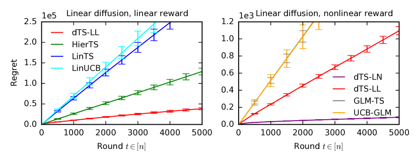
Figure 2: Regret of dTS-LL (Section 3.1.1) and dTS-LN (Section 3.1.2) when $d=20$, $K=10^{4}$ and $n=5000$.

Results for linear diffusion (Figure 2). We begin by examining the case of linear rewards in Figure 2. First, dTS-LL consistently outperforms all baselines that either disregard the latent structure (LinTS and LinUCB) or incorporate it only partially (HierTS). Specifically, the baselines that disregard the structure (LinTS and LinUCB) fail to converge in $n=5000$ rounds since our problem involves a high-dimensional setting with $d=20$ and a large action space of $K=10^{4}$. These baselines appear to require a more extended horizon $n$ for convergence. Meanwhile, HierTS, which partially leverages the structure, manages to converge within the considered horizon but still incurs a significantly higher regret compared to dTS-LL. In contrast, dTS-LL enjoys rapid convergence and maintains low regret.

In the case of non-linear rewards in Figure 2, dTS-LN also surpasses all baselines. Moreover, dTS-LN outperforms dTS-LL in this setting, underscoring the advantages of our approximation in Section 3.1.2. While dTS-LN lacks theoretical guarantees, the results suggest that it is preferable to use dTS-LN when dealing with non-linear rewards, emphasizing the generality and adaptability of dTS and the general posterior derivations in Section 3. However, despite the misspecification of the reward model in dTS-LL, it still outperforms models that use the correct reward model but neglect the latent structure, such as GLM-TS and UCB-GLM. This highlights the importance of accounting for the latent structure, which can outweigh the correctness of the reward model itself in some cases. Finally, we also conduct an additional experiment to verify the impact of the number of actions $K$, the context dimension $d$, and the diffusion depth $L$ on the regret of dTS. The results are in Appendix D and they match Theorem 4.1.

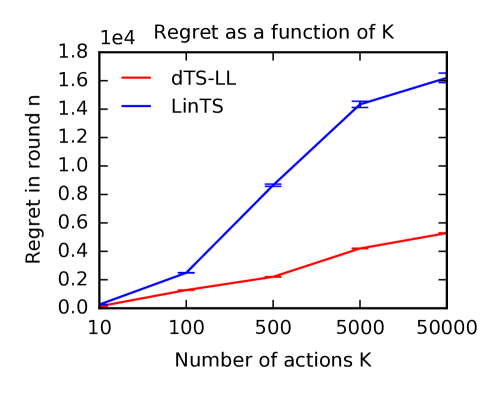
Figure 3: Regret of dTS-LL and LinTS with varying $K$.

Large action spaces (Figure 3). To showcase dTS’s improved scalability to larger action spaces, we examine its performance across a range of $K$ values, from $10$ to $50,000$, in our setting with linear diffusion and rewards (Section 3.1.1). Figure 3 reports the final cumulative regret for varying values of $K$ for both dTS-LL (Section 3.1.1) and LinTS, observing that the gap in the performance becomes larger as $K$ increases.

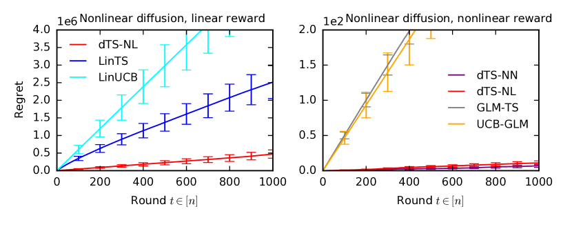
Figure 4: Regret of dTS-NL (Section 3.2.1) and dTS-NN (Section 3.2.2) when $d=20$ and $K=10^{4}$.

Results for non-linear diffusion (Figure 4). We also evaluate our proposed approximation for non-linear diffusion models, with both linear rewards (Section 3.2.1) and non-linear ones (Section 3.2.2). In the linear reward setting, dTS-NL demonstrates significant performance gains compared to both LinTS and LinUCB baselines. With non-linear rewards, dTS-NN surpasses both GLM-TS and UCB-GLM. Furthermore, dTS-NN outperforms dTS-NL in this setting due to its combined use of the correct reward model and the correct latent structure. Similarly to the linear diffusion case previously discussed, dTS-NL surpasses algorithms that employ the correct reward model but neglect the latent structure (GLM-TS and UCB-GLM). The performance gap between dTS-NL and these algorithms is even more pronounced in this non-linear diffusion setting compared to the linear diffusion setting, potentially due to the increased complexity of the latent structure overshadowing the impact of the reward model itself.

6 Conclusion

Grappling with large action spaces in contextual bandits is challenging. Recognizing this, we focused on structured problems where action parameters are sampled from a diffusion model; upon which we built diffusion Thompson sampling (dTS). We developed both theoretical and algorithmic foundations for dTS in numerous practical settings.

We identified several directions for future work. Notably, exploring other approximations for non-linear diffusion models, both empirically and theoretically. From a theoretical perspective, future research could explore the advantages of non-linear diffusion models by deriving their Bayes regret bounds, akin to our analysis in Section 4. Empirically, investigating other approximations and assessing their performance in complex tasks would be interesting. Additionally, exploring the extension of this work to offline (or off-policy) learning in contextual bandits represents a promising avenue for future research.

Broader Impact

This work contributes to the development and analysis of practical algorithms for online learning to act under uncertainty. While our generic setting and algorithms have broad potential applications, the specific downstream social impacts are inherently dependent on the chosen application domain. Nevertheless, we acknowledge the crucial need to consider potential biases that may be present in pre-trained diffusion models, given that our method relies on them.

Supplementary Materials

Notation. For any positive integer $n$, we define $[n]=\{1,2,...,n\}$. Let $v_{1},\ldots,v_{n}\in^{d}$ be $n$ vectors, $(v_{i})_{i\in[n]}\in^{nd}$ is the $nd$-dimensional vector obtained by concatenating $v_{1},\ldots,v_{n}$. For any matrix $\mathrm{A}\in\mathbb{R}^{d\times d}$, $\lambda_{1}(\mathrm{A})$ and $\lambda_{d}(\mathrm{A})$ denote the maximum and minimum eigenvalues of $\mathrm{A}$, respectively. Finally, we write $\tilde{\mathcal{O}}$ for the big-O notation up to polylogarithmic factors.

Appendix A Extended Related Work

Thompson sampling (TS) operates within the Bayesian framework and it involves specifying a prior/likelihood model. In each round, the agent samples unknown model parameters from the current posterior distribution. The chosen action is the one that maximizes the resulting reward. TS is naturally randomized, particularly simple to implement, and has highly competitive empirical performance in both simulated and real-world problems (Russo & Van Roy, 2014; Chapelle & Li, 2012). Regret guarantees for the TS heuristic remained open for decades even for simple models. Recently, however, significant progress has been made. For standard multi-armed bandits, TS is optimal in the Beta-Bernoulli model (Kaufmann et al., 2012; Agrawal & Goyal, 2013b), Gaussian-Gaussian model (Agrawal & Goyal, 2013b), and in the exponential family using Jeffrey’s prior (Korda et al., 2013). For linear bandits, TS is nearly-optimal (Russo & Van Roy, 2014; Agrawal & Goyal, 2017; Abeille & Lazaric, 2017). In this work, we build TS upon complex diffusion priors and analyze the resulting Bayes regret (Russo & Van Roy, 2014) in the linear contextual bandit setting.

Decision-making with diffusion models gained attention recently, especially in offline learning (Ajay et al., 2022; Janner et al., 2022; Wang et al., 2022). However, their application in online learning was only examined by Hsieh et al. (2023), which focused on meta-learning in multi-armed bandits without theoretical guarantees. In this work, we expand the scope of Hsieh et al. (2023) to encompass the broader contextual bandit framework. In particular, we provide theoretical analysis for linear instances, effectively capturing the advantages of using diffusion models as priors in contextual Thompson sampling. These linear cases are particularly captivating due to closed-form posteriors, enabling both theoretical analysis and computational efficiency; an important practical consideration.

Hierarchical Bayesian bandits (Bastani et al., 2019; Kveton et al., 2021; Basu et al., 2021; Simchowitz et al., 2021; Wan et al., 2021; Hong et al., 2022b; Peleg et al., 2022; Wan et al., 2022; Aouali et al., 2023b) applied TS to simple graphical models, wherein action parameters are generally sampled from a Gaussian distribution centered at a single latent parameter. These works mostly span meta- and multi-task learning for multi-armed bandits, except in cases such as Aouali et al. (2023b); Hong et al. (2022a) that consider the contextual bandit setting. Precisely, Aouali et al. (2023b) assume that action parameters are sampled from a Gaussian distribution centered at a linear mixture of multiple latent parameters. On the other hand, Hong et al. (2022a) applied TS to a graphical model represented by a tree. Our work can be seen as an extension of all these works to much more complex graphical models, for which both theoretical and algorithmic foundations are developed. Note that the settings in most of these works can be recovered with specific choices of the diffusion depth $L$ and functions $f_{\ell}$. This attests to the modeling power of dTS.

Approximate Thompson sampling is a major problem in the Bayesian inference literature. This is because most posterior distributions are intractable, and thus practitioners must resort to sophisticated computational techniques such as Markov chain Monte Carlo (Kruschke, 2010). Prior works (Riquelme et al., 2018; Chapelle & Li, 2012; Kveton et al., 2020) highlight the favorable empirical performance of approximate Thompson sampling. Particularly, (Kveton et al., 2020) provide theoretical guarantees for Thompson sampling when using the Laplace approximation in generalized linear bandits (GLB). In our context, we incorporate approximate sampling when the reward exhibits non-linearity. While our approximation does not come with formal guarantees, it enjoys strong practical performance. An in-depth analysis of this approximation is left as a direction for future works. Similarly, approximating the posterior distribution when the diffusion model is non-linear as well as analyzing it is an interesting direction of future works.

Bandits with underlying structure also align with our work, where we assume a structured relationship among actions, captured by a diffusion model. In latent bandits (Maillard & Mannor, 2014; Hong et al., 2020), a single latent variable indexes multiple candidate models. Within structured finite-armed bandits (Lattimore & Munos, 2014; Gupta et al., 2018), each action is linked to a known mean function parameterized by a common latent parameter. This latent parameter is learned. TS was also applied to complex structures (Yu et al., 2020; Gopalan et al., 2014). However, simultaneous computational and statistical efficiencies aren’t guaranteed. Meta- and multi-task learning with upper confidence bound (UCB) approaches have a long history in bandits (Azar et al., 2013; Gentile et al., 2014; Deshmukh et al., 2017; Cella et al., 2020). These, however, often adopt a frequentist perspective, analyze a stronger form of regret, and sometimes result in conservative algorithms. In contrast, our approach is Bayesian, with analysis centered on Bayes regret. Remarkably, our algorithm, dTS, performs well as analyzed without necessitating additional tuning. Finally, Low-rank bandits (Hu et al., 2021; Cella et al., 2022; Yang et al., 2020) also relate to our linear diffusion model when $L=1$. Broadly, there exist two key distinctions between these prior works and the special case of our model (linear diffusion model with $L=1$). First, they assume $\theta_{*,i}=\mathrm{W}_{1}\psi_{*,1}$, whereas we incorporate additional uncertainty in the covariance $\Sigma_{1}$ to account for possible misspecification as $\theta_{*,i}=\mathcal{N}(\mathrm{W}_{1}\psi_{*,1},\Sigma_{1})$. Consequently, these algorithms might suffer linear regret due to model misalignment. Second, we assume that the mixing matrix $\mathrm{W}_{1}$ is available and pre-learned offline, whereas they learn it online. While this is more general, it leads to computationally expensive methods that are difficult to employ in a real-world online setting.

Large action spaces. Roughly speaking, the regret bound of dTS scales with $K\sigma_{1}^{2}$ rather than $K\sum_{\ell}\sigma_{\ell}^{2}$. This is particularly beneficial when $\sigma_{1}$ is small, a common scenario in diffusion models with decreasing variances. A notable case is when $\sigma_{1}=0$, where the regret becomes independent of $K$. Also, our analysis (Section 4.1) indicates that the gap in performance between dTS and LinTS becomes more pronounced when the number of action increases, highlighting dTS’s suitability for large action spaces. Note that some prior works (Foster et al., 2020; Xu & Zeevi, 2020; Zhu et al., 2022) proposed bandit algorithms that do not scale with $K$. However, our setting differs significantly from theirs, explaining our inherent dependency on $K$ when $\sigma_{1}>0$. Precisely, they assume a reward function of $r(x,i)=\phi(x,i)^{\top}\theta_{*}$, with a shared $\theta_{*}\in\mathbb{R}^{d}$ across actions and a known mapping $\phi$. In contrast, we consider $r(x,i)=x^{\top}\theta_{*,i}$, requiring the learning of $K$ separate $d$-dimensional action parameters. In their setting, with the availability of $\phi$, the regret of dTS would similarly be independent of $K$. However, obtaining such a mapping $\phi$ can be challenging as it needs to encapsulate complex context-action dependencies. Notably, our setting reflects a common practical scenario, such as in recommendation systems where each product is often represented by its embedding. In summary, the dependency on $K$ is more related to our setting than the method itself, and dTS would scale with $d$ only in their setting. Note that dTS is both computationally and statistically efficient (Section 4.1). This becomes particularly notable in large action spaces. Our empirical results in Figure 2, notably with $K=10^{4}$, demonstrate that dTS significantly outperforms the baselines. More importantly, the performance gap between dTS and these baselines is larger when the number of actions ($K$) increases, highlighting the improved scalability of dTS to large action spaces.

Bayesian analyses in contextual bandits. Traditionally, contextual bandit algorithms are evaluated using frequentist regret, which measures the performance against a fixed but unknown environment parameter $\theta_{*}$. This approach assumes no prior knowledge about $\theta_{*}$. In contrast, Bayesian regret (Russo & Van Roy, 2014) assumes that $\theta_{*}$ is drawn from a known prior distribution. The Bayesian regret then calculates the average regret across all possible values of $\theta_{*}$ sampled from the prior. This work employs Bayesian regret because it allows us to leverage informative priors (Hong et al., 2022b; Aouali et al., 2023b). Interestingly, PAC-Bayesian theory also offers a Bayesian perspective and has seen success in capturing the benefits of prior information, as it was demonstrated in offline contextual bandits (London & Sandler, 2019; Sakhi et al., 2023; Aouali et al., 2023a). However, this work does not employ PAC-Bayesian analysis, and a connection between PAC-Bayesian theory and Bayesian regret remains unclear.

Appendix B Derivation of Closed-Form Posteriors for Linear Diffusion Models

In this section, we derive the $K+L$ posteriors $P_{t,i}$ and $Q_{t,\ell}$, for which we provide the expressions in Section 3.1. In our proofs, $p(x)\propto f(x)$ means that the probability density $p$ satisfies $p(x)=\frac{f(x)}{Z}$ for any $x\in^{d}$, where $Z$ is a normalization constant. In particular, we extensively use that if $p(x)\propto\exp[-\frac{1}{2}x^{\top}\Lambda x+x^{\top}m]$, where $\Lambda$ is positive definite. Then $p$ is the multivariate Gaussian density with covariance $\Sigma=\Lambda^{-1}$ and mean $\mu=\Sigma m$. These are standard notations and techniques to manipulate Gaussian distributions (Koller & Friedman, 2009, Chapter 7). We note that the posterior derivations in this section are similar to those used in linear Gaussian systems (Bishop, 2006).

B.1 Derivation of Action-Posteriors for Linear Diffusion Models

Proposition B.1.

Consider the following model, which corresponds to the last two layers in (4)

$$\theta_{*,i}\mid\psi_{*,1} \sim\mathcal{N}\left(\mathrm{W}_{1}\psi_{*,1},\Sigma_{1}\right)\,,$$

$$Y_{t}\mid X_{t},\theta_{*,A_{t}} \sim\mathcal{N}\left(X_{t}^{\top}\theta_{*,A_{t}},\sigma^{2}\right)\,, \forall t\in[n]\,.$$

Then we have that for any $t\in[n]$ and $i\in[K]$, $P_{t,i}(\theta\mid\psi_{1})=\mathbb{P}\left(\theta_{*,i}=\theta\,\middle|\,\psi_{*,1}=\psi_{1},H_{t,i}\right)=\mathcal{N}(\theta;\hat{\mu}_{t,i},\hat{\Sigma}_{t,i})$, where

$$\hat{\Sigma}^{-1}_{t,i}=\hat{G}_{t,i}+\Sigma_{1}^{-1}\,, \hat{\mu}_{t,i} =\hat{\Sigma}_{t,i}\left(\hat{B}_{t,i}+\Sigma_{1}^{-1}\mathrm{W}_{1}\psi_{1}\right)\,.$$

Proof.

Let $v=\sigma^{-2}\,,\quad\Lambda_{1}=\Sigma_{1}^{-1}\,.$ Then the action-posterior decomposes as

$$P_{t,i}(\theta\mid\psi_{1}) =\mathbb{P}\left(\theta_{*,i}=\theta\,\middle|\,\psi_{*,1}=\psi_{1},H_{t,i}\right)\,,$$

$$\propto\mathbb{P}\left(H_{t,i}\,\middle|\,\psi_{*,1}=\psi_{1},\theta_{*,i}=\theta\right)\mathbb{P}\left(\theta_{*,i}=\theta\,\middle|\,\psi_{*,1}=\psi_{1}\right)\,,\quad(\text{Bayes rule})$$

$$=\mathbb{P}\left(H_{t,i}\,\middle|\,\theta_{*,i}=\theta\right)\mathbb{P}\left(\theta_{*,i}=\theta\,\middle|\,\psi_{*,1}=\psi_{1}\right)\,,(\text{given $\theta_{*,i}$, $H_{t,i}$ is independent of $\psi_{*,1}$})$$

$$=\prod_{k\in S_{t,i}}\mathcal{N}(Y_{k};X_{k}^{\top}\theta,\sigma^{2})\mathcal{N}(\theta;\mathrm{W}_{1}\psi_{1},\Sigma_{1})\,,$$

$$=\exp\Big{[}-\frac{1}{2}\Big{(}v\sum_{k\in S_{t,i}}(Y_{k}^{2}-2Y_{k}X_{k}^{\top}\theta+(X_{k}^{\top}\theta)^{2})+\theta^{\top}\Lambda_{1}\theta-2\theta^{\top}\Lambda_{1}\mathrm{W}_{1}\psi_{1}$$

$$\qquad\qquad+\big{(}\mathrm{W}_{1}\psi_{1}\big{)}^{\top}\Lambda_{1}\big{(}\mathrm{W}_{1}\psi_{1}\big{)}\Big{)}\Big{]}\,,$$

$$\propto\exp\Big{[}-\frac{1}{2}\Big{(}\theta^{\top}(v\sum_{k\in S_{t,i}}X_{k}X_{k}^{\top}+\Lambda_{1})\theta-2\theta^{\top}\Big{(}v\sum_{k\in S_{t,i}}X_{k}Y_{k}+\Lambda_{1}\mathrm{W}_{1}\psi_{1}\Big{)}\Big{)}\Big{]}\,,$$

$$\propto\mathcal{N}\big{(}\theta;\hat{\mu}_{t,i},\hat{\Lambda}_{t,i}^{-1}\big{)}\,,$$

where $\hat{\Lambda}_{t,i}=v\sum_{k\in S_{t,i}}X_{k}X_{k}^{\top}+\Lambda_{1}\,,$ and $\hat{\Lambda}_{t,i}\hat{\mu}_{t,i}=v\sum_{k\in S_{t,i}}X_{k}Y_{k}+\Lambda_{1}\mathrm{W}_{1}\psi_{1}$. Using that $\hat{B}_{t,i}=v\sum_{k\in S_{t,i}}X_{k}Y_{k}$ and $\hat{G}_{t,i}=v\sum_{k\in S_{t,i}}X_{k}X_{k}^{\top}$ concludes the proof. ∎

B.2 Derivation of Recursive Latent-Posteriors for Linear Diffusion Models

Proposition B.2.

For any $\ell\in[L]/\{1\}$, the $\ell-1$-th conditional latent-posterior reads $Q_{t,\ell-1}(\cdot\mid\psi_{\ell})=\mathcal{N}(\bar{\mu}_{t,\ell-1},\bar{\Sigma}_{t,\ell-1})$, with

$$\bar{\Sigma}_{t,\ell-1}^{-1}=\Sigma_{\ell}^{-1}+\bar{G}_{t,\ell-1}\,, \bar{\mu}_{t,\ell-1}=\bar{\Sigma}_{t,\ell-1}\big{(}\Sigma_{\ell}^{-1}\mathrm{W}_{\ell}\psi_{\ell}+\bar{B}_{t,\ell-1}\big{)}\,,$$ (17)

and the $L$-th latent-posterior reads $Q_{t,L}(\cdot)=\mathcal{N}(\bar{\mu}_{t,L},\bar{\Sigma}_{t,L})$, with

$$\bar{\Sigma}_{t,L}^{-1}=\Sigma_{L+1}^{-1}+\bar{G}_{t,L}\,, \bar{\mu}_{t,L}=\bar{\Sigma}_{t,L}\bar{B}_{t,L}\,.$$ (18)

Proof.

Let $\ell\in[L]/\{1\}$. Then, Bayes rule yields that

$$Q_{t,\ell-1}(\psi_{\ell-1}\mid\psi_{\ell}) \propto\mathbb{P}\left(H_{t}\,\middle|\,\psi_{*,\ell-1}=\psi_{\ell-1}\right)\mathcal{N}(\psi_{\ell-1},\mathrm{W}_{\ell}\psi_{\ell},\Sigma_{\ell})\,,$$

But from Lemma B.3, we know that

$$\mathbb{P}\left(H_{t}\,\middle|\,\psi_{*,\ell-1}=\psi_{\ell-1}\right)\propto\exp\Big{[}-\frac{1}{2}\psi_{\ell-1}^{\top}\bar{G}_{t,\ell-1}\psi_{\ell-1}+\psi_{\ell-1}^{\top}\bar{B}_{t,\ell-1}\Big{]}\,.$$

Therefore,

$$Q_{t,\ell-1}(\psi_{\ell-1}\mid\psi_{\ell}) \propto\exp\Big{[}-\frac{1}{2}\psi_{\ell-1}^{\top}\bar{G}_{t,\ell-1}\psi_{\ell-1}+\psi_{\ell-1}^{\top}\bar{B}_{t,\ell-1}\Big{]}\mathcal{N}(\psi_{\ell-1},\mathrm{W}_{\ell}\psi_{\ell},\Sigma_{\ell})\,,$$

$$\propto\exp\Big{[}-\frac{1}{2}\psi_{\ell-1}^{\top}\bar{G}_{t,\ell-1}\psi_{\ell-1}+\psi_{\ell-1}^{\top}\bar{B}_{t,\ell-1}$$

$$\qquad\qquad-\frac{1}{2}(\psi_{\ell-1}-\mathrm{W}_{\ell}\psi_{\ell})^{\top}\Sigma_{\ell}^{-1}(\psi_{\ell-1}-\mathrm{W}_{\ell}\psi_{\ell}))\Big{]}\,,$$

$$\stackrel{{\scriptstyle(i)}}{{\propto}}\exp\Big{[}-\frac{1}{2}\psi_{\ell-1}^{\top}(\bar{G}_{t,\ell-1}+\Sigma_{\ell}^{-1})\psi_{\ell-1}+\psi_{\ell-1}^{\top}(\bar{B}_{t,\ell-1}+\Sigma_{\ell}^{-1}\mathrm{W}_{\ell}\psi_{\ell})\Big{]}\,,$$

$$\stackrel{{\scriptstyle(ii)}}{{\propto}}\mathcal{N}(\psi_{\ell-1};\bar{\mu}_{t,\ell-1},\bar{\Sigma}_{t,\ell-1})\,,$$

with $\bar{\Sigma}_{t,\ell-1}^{-1}=\Sigma_{\ell}^{-1}+\bar{G}_{t,\ell-1}$ and $\bar{\mu}_{t,\ell-1}=\bar{\Sigma}_{t,\ell-1}\big{(}\Sigma_{\ell}^{-1}\mathrm{W}_{\ell}\psi_{\ell}+\bar{B}_{t,\ell-1}\big{)}$. In $(i)$, we omit terms that are constant in $\psi_{\ell-1}$. In $(ii)$, we complete the square. This concludes the proof for $\ell\in[L]/\{1\}$. For $Q_{t,L}$, we use Bayes rule to get

$$Q_{t,L}(\psi_{L}) \propto\mathbb{P}\left(H_{t}\,\middle|\,\psi_{*,L}=\psi_{L}\right)\mathcal{N}(\psi_{L},0,\Sigma_{L+1})\,.$$

Then from Lemma B.3, we know that

$$\mathbb{P}\left(H_{t}\,\middle|\,\psi_{*,L}=\psi_{L}\right)\propto\exp\Big{[}-\frac{1}{2}\psi_{L}^{\top}\bar{G}_{t,L}\psi_{L}+\psi_{L}^{\top}\bar{B}_{t,L}\Big{]}\,,$$

We then use the same derivations above to compute the product $\exp\Big{[}-\frac{1}{2}\psi_{L}^{\top}\bar{G}_{t,L}\psi_{L}+\psi_{L}^{\top}\bar{B}_{t,L}\Big{]}\times\mathcal{N}(\psi_{L},0,\Sigma_{L+1})$, which concludes the proof. ∎

Lemma B.3.

The following holds for any $t\in[n]$ and $\ell\in[L]$,

$$\mathbb{P}\left(H_{t}\,\middle|\,\psi_{*,\ell}=\psi_{\ell}\right)\propto\exp\Big{[}-\frac{1}{2}\psi_{\ell}^{\top}\bar{G}_{t,\ell}\psi_{\ell}+\psi_{\ell}^{\top}\bar{B}_{t,\ell}\Big{]}\,,$$

where $\bar{G}_{t,\ell}$ and $\bar{B}_{t,\ell}$ are defined by recursion in Section 3.1.

Proof.

We prove this result by induction. To reduce clutter, we let $v=\sigma^{-2}$, and $\Lambda_{1}=\Sigma_{1}^{-1}$. We start with the base case of the induction when $\ell=1$.

(I) Base case. Here we want to show that $\mathbb{P}\left(H_{t}\,\middle|\,\psi_{*,1}=\psi_{1}\right)\propto\exp\Big{[}-\frac{1}{2}\psi_{1}^{\top}\bar{G}_{t,1}\psi_{1}+\psi_{1}^{\top}\bar{B}_{t,1}\big{)}\Big{]}$, where $\bar{G}_{t,1}$ and $\bar{B}_{t,1}$ are given in (3.1.1). First, we have that

$$\mathbb{P}\left(H_{t}\,\middle|\,\psi_{*,1}=\psi_{1}\right) \stackrel{{\scriptstyle(i)}}{{=}}\prod_{i\in[K]}\mathbb{P}\left(H_{t,i}\,\middle|\,\psi_{*,1}=\psi_{1}\right)=\prod_{i\in[K]}\int_{\theta}\mathbb{P}\left(H_{t,i},\theta_{*,i}=\theta\,\middle|\,\psi_{*,1}=\psi_{1}\right)\mathop{}\!\mathrm{d}\theta\,,$$

$$=\prod_{i\in[K]}\int_{\theta}\mathbb{P}\left(H_{t,i}\,\middle|\,\theta_{*,i}=\theta\right)\mathcal{N}\left(\theta;\mathrm{W}_{1}\psi_{1},\Sigma_{1}\right)\mathop{}\!\mathrm{d}\theta\,,$$

$$=\prod_{i\in[K]}\underbrace{\int_{\theta}\Big{(}\prod_{k\in S_{t,i}}\mathcal{N}(Y_{k};X_{k}^{\top}\theta,\sigma^{2})\Big{)}\mathcal{N}\left(\theta;\mathrm{W}_{1}\psi_{1},\Sigma_{1}\right)\mathop{}\!\mathrm{d}\theta}_{h_{i}(\psi_{1})}\,,$$

$$=\prod_{i\in[K]}h_{i}(\psi_{1})\,,$$ (19)

where $(i)$ follows from the fact that $\theta_{*,i}$ for $i\in[K]$ are conditionally independent given $\psi_{*,1}=\psi_{1}$ and that given $\theta_{*,i}$, $H_{t,i}$ is independent of $\psi_{*,1}$. Now we compute $h_{i}(\psi_{1})=\int_{\theta}\left(\prod_{k\in S_{t,i}}\mathcal{N}(Y_{k};X_{k}^{\top}\theta,\sigma^{2})\right)\mathcal{N}\left(\theta;\mathrm{W}_{1}\psi_{1},\Sigma_{1}\right)\mathop{}\!\mathrm{d}\theta$ as

$$h_{i}(\psi_{1})=\int_{\theta}\Big{(}\prod_{k\in S_{t,i}}\mathcal{N}(Y_{k};X_{k}^{\top}\theta,\sigma^{2})\Big{)}\mathcal{N}(\theta;\mathrm{W}_{1}\psi_{1},\Sigma_{1})\mathop{}\!\mathrm{d}\theta\,,$$

$$\propto\int_{\theta}\exp\Big{[}-\frac{1}{2}v\sum_{k\in S_{t,i}}(Y_{k}-X_{k}^{\top}\theta)^{2}-\frac{1}{2}(\theta-\mathrm{W}_{1}\psi_{1})^{\top}\Lambda_{1}(\theta-\mathrm{W}_{1}\psi_{1})\Big{]}\mathop{}\!\mathrm{d}\theta\,,$$

$$=\int_{\theta}\exp\Big{[}-\frac{1}{2}\Big{(}v\sum_{k\in S_{t,i}}(Y_{k}^{2}-2Y_{k}\theta^{\top}X_{k}+(\theta^{\top}X_{k})^{2})+\theta^{\top}\Lambda_{1}\theta-2\theta^{\top}\Lambda_{1}\mathrm{W}_{1}\psi_{1}$$

$$\qquad\qquad+(\mathrm{W}_{1}\psi_{1})^{\top}\Lambda_{1}(\mathrm{W}_{1}\psi_{1})\Big{)}\Big{]}\mathop{}\!\mathrm{d}\theta\,,$$

$$\propto\int_{\theta}\exp\Big{[}-\frac{1}{2}\Big{(}\theta^{\top}\Big{(}v\sum_{k\in S_{t,i}}X_{k}X_{k}^{\top}+\Lambda_{1}\Big{)}\theta-2\theta^{\top}\Big{(}v\sum_{k\in S_{t,i}}Y_{k}X_{k}$$

$$\qquad\qquad+\Lambda_{1}\mathrm{W}_{1}\psi_{1}\Big{)}+(\mathrm{W}_{1}\psi_{1})^{\top}\Lambda_{1}(\mathrm{W}_{1}\psi_{1})\Big{)}\Big{]}\mathop{}\!\mathrm{d}\theta\,.$$

But we know that $\hat{G}_{t,i}=v\sum_{k\in S_{t,i}}X_{k}X_{k}^{\top}$, and $\hat{B}_{t,i}=v\sum_{k\in S_{t,i}}Y_{k}X_{k}$. To further simplify expressions, we also let

$$V=\big{(}\hat{G}_{t,i}+\Lambda_{1}\big{)}^{-1}\,,\quad U=V^{-1}\,,\quad\beta=V\big{(}\hat{B}_{t,i}+\Lambda_{1}\mathrm{W}_{1}\psi_{1}\big{)}\,.$$

We have that $UV=VU=I_{d}\,,$ and thus

$$h_{i}(\psi_{1}) \propto\int_{\theta}\exp\left[-\frac{1}{2}\left(\theta^{\top}U\theta-2\theta^{\top}UV\left(\hat{B}_{t,i}+\Lambda_{1}\mathrm{W}_{1}\psi_{1}\right)+(\mathrm{W}_{1}\psi_{1})^{\top}\Lambda_{1}(\mathrm{W}_{1}\psi_{1})\right)\right]\mathop{}\!\mathrm{d}\theta\,,$$

$$=\int_{\theta}\exp\left[-\frac{1}{2}\left(\theta^{\top}U\theta-2\theta^{\top}U\beta+(\mathrm{W}_{1}\psi_{1})^{\top}\Lambda_{1}(\mathrm{W}_{1}\psi_{1})\right)\right]\mathop{}\!\mathrm{d}\theta\,,$$

$$=\int_{\theta}\exp\left[-\frac{1}{2}\left((\theta-\beta)^{\top}U(\theta-\beta)-\beta^{\top}U\beta+(\mathrm{W}_{1}\psi_{1})^{\top}\Lambda_{1}(\mathrm{W}_{1}\psi_{1})\right)\right]\mathop{}\!\mathrm{d}\theta\,,$$

$$\propto\exp\left[-\frac{1}{2}\left(-\beta^{\top}U\beta+(\mathrm{W}_{1}\psi_{1})^{\top}\Lambda_{1}(\mathrm{W}_{1}\psi_{1})\right)\right]\,,$$

$$=\exp\left[-\frac{1}{2}\left(-\left(\hat{B}_{t,i}+\Lambda_{1}\mathrm{W}_{1}\psi_{1}\right)^{\top}V\left(\hat{B}_{t,i}+\Lambda_{1}\mathrm{W}_{1}\psi_{1}\right)+(\mathrm{W}_{1}\psi_{1})^{\top}\Lambda_{1}(\mathrm{W}_{1}\psi_{1})\right)\right]\,,$$

$$\propto\exp\left[-\frac{1}{2}\left(\psi_{1}^{\top}\mathrm{W}_{1}^{\top}\left(\Lambda_{1}-\Lambda_{1}V\Lambda_{1}\right)\mathrm{W}_{1}\psi_{1}-2\psi_{1}^{\top}\left(\mathrm{W}_{1}^{\top}\Lambda_{1}V\hat{B}_{t,i}\right)\right)\right]\,,$$

$$=\exp\left[-\frac{1}{2}\psi_{1}^{\top}\Omega_{i}\psi_{1}+\psi_{1}^{\top}m_{i}\right]\,,$$

where

$$\Omega_{i} =\mathrm{W}_{1}^{\top}\left(\Lambda_{1}-\Lambda_{1}V\Lambda_{1}\right)\mathrm{W}_{1}=\mathrm{W}_{1}^{\top}\left(\Lambda_{1}-\Lambda_{1}(\hat{G}_{t,i}+\Lambda_{1})^{-1}\Lambda_{1}\right)\mathrm{W}_{1}\,,$$

$$m_{i} =\mathrm{W}_{1}^{\top}\Lambda_{1}V\hat{B}_{t,i}=\mathrm{W}_{1}^{\top}\Lambda_{1}(\hat{G}_{t,i}+\Lambda_{1})^{-1}\hat{B}_{t,i}\,.$$ (20)

But notice that $V=(\hat{G}_{t,i}+\Lambda_{1})^{-1}=\hat{\Sigma}_{t,i}$ and thus

$$\Omega_{i}=\mathrm{W}_{1}^{\top}\big{(}\Lambda_{1}-\Lambda_{1}\hat{\Sigma}_{t,i}\Lambda_{1}\big{)}\mathrm{W}_{1}\,, m_{i} =\mathrm{W}_{1}^{\top}\Lambda_{1}\hat{\Sigma}_{t,i}\hat{B}_{t,i}\,.$$ (21)

Finally, we plug this result in (B.2) to get

$$\mathbb{P}\left(H_{t}\,\middle|\,\psi_{*,1}=\psi_{1}\right)=\prod_{i\in[K]}h_{i}(\psi_{1}) \propto\prod_{i\in[K]}\exp\left[-\frac{1}{2}\psi_{1}^{\top}\Omega_{i}\psi_{1}+\psi_{1}^{\top}m_{i}\right]\,,$$

$$=\exp\left[-\frac{1}{2}\psi_{1}^{\top}\sum_{i\in[K]}\Omega_{i}\psi_{1}+\psi_{1}^{\top}\sum_{i\in[K]}m_{i}\right]\,,$$

$$=\exp\left[-\frac{1}{2}\psi_{1}^{\top}\bar{G}_{t,1}\psi_{1}+\psi_{1}^{\top}\bar{B}_{t,1}\right]\,,$$

where

$$\bar{G}_{t,1} =\sum_{i=1}^{K}\Omega_{i}=\sum_{i=1}^{K}\mathrm{W}_{1}^{\top}\big{(}\Lambda_{1}-\Lambda_{1}\hat{\Sigma}_{t,i}\Lambda_{1}\big{)}\mathrm{W}_{1}=\mathrm{W}_{1}^{\top}\sum_{i=1}^{K}\big{(}\Sigma_{1}^{-1}-\Sigma_{1}^{-1}\hat{\Sigma}_{t,i}\Sigma_{1}^{-1}\big{)}\mathrm{W}_{1}\,,$$

$$\bar{B}_{t,1} =\sum_{i=1}^{K}m_{i}=\sum_{i=1}^{K}\hat{\Sigma}_{t,i}\hat{B}_{t,i}=\mathrm{W}_{1}^{\top}\Sigma_{1}^{-1}\sum_{i=1}^{K}\hat{\Sigma}_{t,i}\hat{B}_{t,i}\,.$$

This concludes the proof of the base case.

(II) Induction step. Let $\ell\in[L]/\{1\}$. Suppose that

$$\mathbb{P}\left(H_{t}\,\middle|\,\psi_{*,\ell-1}=\psi_{\ell-1}\right)\propto\exp\left[-\frac{1}{2}\psi_{\ell-1}^{\top}\bar{G}_{t,\ell-1}\psi_{\ell-1}+\psi_{\ell-1}^{\top}\bar{B}_{t,\ell-1}\right]\,.$$ (22)

Then we want to show that

$$\mathbb{P}\left(H_{t}\,\middle|\,\psi_{*,\ell}=\psi_{\ell}\right)\propto\exp\left[-\frac{1}{2}\psi_{\ell}^{\top}\bar{G}_{t,\ell}\psi_{\ell}+\psi_{\ell}^{\top}\bar{B}_{t,\ell}\right]\,,$$

where

$$\bar{G}_{t,\ell} =\mathrm{W}_{\ell}^{\top}\big{(}\Sigma_{\ell}^{-1}-\Sigma_{\ell}^{-1}\bar{\Sigma}_{t,\ell-1}\Sigma_{\ell}^{-1}\big{)}\mathrm{W}_{\ell}=\mathrm{W}_{\ell}^{\top}\big{(}\Sigma_{\ell}^{-1}-\Sigma_{\ell}^{-1}(\Sigma_{\ell}^{-1}+\bar{G}_{t,\ell-1})^{-1}\Sigma_{\ell}^{-1}\big{)}\mathrm{W}_{\ell}\,,$$

$$\bar{B}_{t,\ell} =\mathrm{W}_{\ell}^{\top}\Sigma_{\ell}^{-1}\bar{\Sigma}_{t,\ell-1}\bar{B}_{t,\ell-1}=\mathrm{W}_{\ell}^{\top}\Sigma_{\ell}^{-1}(\Sigma_{\ell}^{-1}+\bar{G}_{t,\ell-1})^{-1}\bar{B}_{t,\ell-1}\,.$$

To achieve this, we start by expressing $\mathbb{P}\left(H_{t}\,\middle|\,\psi_{*,\ell}=\psi_{\ell}\right)$ in terms of $\mathbb{P}\left(H_{t}\,\middle|\,\psi_{*,\ell-1}=\psi_{\ell-1}\right)$ as

$$\mathbb{P}\left(H_{t}\,\middle|\,\psi_{*,\ell}=\psi_{\ell}\right)=\int_{\psi_{\ell-1}}\mathbb{P}\left(H_{t},\psi_{*,\ell-1}=\psi_{\ell-1}\,\middle|\,\psi_{*,\ell}=\psi_{\ell}\right)\mathop{}\!\mathrm{d}\psi_{\ell-1}\,,$$

$$=\int_{\psi_{\ell-1}}\mathbb{P}\left(H_{t}\,\middle|\,\psi_{*,\ell-1}=\psi_{\ell-1},\psi_{*,\ell}=\psi_{\ell}\right)\mathcal{N}(\psi_{\ell-1};\mathrm{W}_{\ell}\psi_{\ell},\Sigma_{\ell})\mathop{}\!\mathrm{d}\psi_{\ell-1}\,,$$

$$=\int_{\psi_{\ell-1}}\mathbb{P}\left(H_{t}\,\middle|\,\psi_{*,\ell-1}=\psi_{\ell-1}\right)\mathcal{N}(\psi_{\ell-1};\mathrm{W}_{\ell}\psi_{\ell},\Sigma_{\ell})\mathop{}\!\mathrm{d}\psi_{\ell-1}\,,$$

$$\propto\int_{\psi_{\ell-1}}\exp\Big{[}-\frac{1}{2}\psi_{\ell-1}^{\top}\bar{G}_{t,\ell-1}\psi_{\ell-1}+\psi_{\ell-1}^{\top}\bar{B}_{t,\ell-1}\Big{]}\mathcal{N}(\psi_{\ell-1};\mathrm{W}_{\ell}\psi_{\ell},\Sigma_{\ell})\mathop{}\!\mathrm{d}\psi_{\ell-1}\,,$$

$$\propto\int_{\psi_{\ell-1}}\exp\Big{[}-\frac{1}{2}\psi_{\ell-1}^{\top}\bar{G}_{t,\ell-1}\psi_{\ell-1}+\psi_{\ell-1}^{\top}\bar{B}_{t,\ell-1}$$

$$\qquad\qquad+(\psi_{\ell-1}-\mathrm{W}_{\ell}\psi_{\ell})^{\top}\Lambda_{\ell}(\psi_{\ell-1}-\mathrm{W}_{\ell}\psi_{\ell})\Big{)}\Big{]}\mathop{}\!\mathrm{d}\psi_{\ell-1}\,.$$

Now let $S=\bar{G}_{t,\ell-1}+\Lambda_{\ell}$ and $V=\bar{B}_{t,\ell-1}+\Lambda_{\ell}\mathrm{W}_{\ell}\psi_{\ell}$. Then we have that,

$$\mathbb{P}\left(H_{t}\,\middle|\,\psi_{*,\ell}=\psi_{\ell}\right)$$

$$\propto\int_{\psi_{\ell-1}}\exp\Big{[}-\frac{1}{2}\psi_{\ell-1}^{\top}\bar{G}_{t,\ell-1}\psi_{\ell-1}+\psi_{\ell-1}^{\top}\bar{B}_{t,\ell-1}$$

$$\qquad\qquad+(\psi_{\ell-1}-\mathrm{W}_{\ell}\psi_{\ell})^{\top}\Lambda_{\ell}(\psi_{\ell-1}-\mathrm{W}_{\ell}\psi_{\ell})\Big{)}\Big{]}\mathop{}\!\mathrm{d}\psi_{\ell-1}\,,$$

$$\propto\int_{\psi_{\ell-1}}\exp\Big{[}-\frac{1}{2}\Big{(}\psi_{\ell-1}^{\top}S\psi_{\ell-1}-2\psi_{\ell-1}^{\top}\left(\bar{B}_{t,\ell-1}+\Lambda_{\ell}\mathrm{W}_{\ell}\psi_{\ell}\right)+\psi_{\ell}^{\top}\mathrm{W}_{\ell}^{\top}\Lambda_{\ell}\mathrm{W}_{\ell}\psi_{\ell}\Big{)}\Big{]}\mathop{}\!\mathrm{d}\psi_{\ell-1}\,,$$

$$=\int_{\psi_{\ell-1}}\exp\Big{[}-\frac{1}{2}\Big{(}\psi_{\ell-1}^{\top}S(\psi_{\ell-1}-2S^{-1}V)+\psi_{\ell}^{\top}\mathrm{W}_{\ell}^{\top}\Lambda_{\ell}\mathrm{W}_{\ell}\psi_{\ell}\Big{)}\Big{]}\mathop{}\!\mathrm{d}\psi_{\ell-1}\,,$$

$$=\int_{\psi_{\ell-1}}\exp\Big{[}-\frac{1}{2}\Big{(}(\psi_{\ell-1}-S^{-1}V)^{\top}S(\psi_{\ell-1}-S^{-1}V)$$

$$\qquad\qquad+\psi_{\ell}^{\top}\mathrm{W}_{\ell}^{\top}\Lambda_{\ell}\mathrm{W}_{\ell}\psi_{\ell}-V^{\top}S^{-1}V\Big{)}\Big{]}\mathop{}\!\mathrm{d}\psi_{\ell-1}.$$

In the second step, we omit constants in $\psi_{\ell}$ and $\psi_{\ell-1}$. Thus

$$\mathbb{P}\left(H_{t}\,\middle|\,\psi_{*,\ell}=\psi_{\ell}\right)$$

$$\propto\int_{\psi_{\ell-1}}\exp\left[-\frac{1}{2}\left((\psi_{\ell-1}-S^{-1}V)^{\top}S(\psi_{\ell-1}-S^{-1}V)+\psi_{\ell}^{\top}\mathrm{W}_{\ell}^{\top}\Lambda_{\ell}\mathrm{W}_{\ell}\psi_{\ell}-V^{\top}S^{-1}V\right)\right]\mathop{}\!\mathrm{d}\psi_{\ell-1},$$

$$\propto\exp\left[-\frac{1}{2}\left(\psi_{\ell}^{\top}\mathrm{W}_{\ell}^{\top}\Lambda_{\ell}\mathrm{W}_{\ell}\psi_{\ell}-V^{\top}S^{-1}V\right)\right]\,.$$

It follows that

$$\mathbb{P}\left(H_{t}\,\middle|\,\psi_{*,\ell}=\psi_{\ell}\right)$$

$$\propto\exp\left[-\frac{1}{2}\left(\psi_{\ell}^{\top}\mathrm{W}_{\ell}^{\top}\Lambda_{\ell}\mathrm{W}_{\ell}\psi_{\ell}-V^{\top}S^{-1}V\right)\right]\,,$$

$$=\exp\left[-\frac{1}{2}\left(\psi_{\ell}^{\top}\mathrm{W}_{\ell}^{\top}\Lambda_{\ell}\mathrm{W}_{\ell}\psi_{\ell}-\left(\bar{B}_{t,\ell-1}+\Lambda_{\ell}\mathrm{W}_{\ell}\psi_{\ell}\right)^{\top}S^{-1}\left(\bar{B}_{t,\ell-1}+\Lambda_{\ell}\mathrm{W}_{\ell}\psi_{\ell}\right)\right)\right]$$

$$\propto\exp\left[-\frac{1}{2}\left(\psi_{\ell}^{\top}\left(\mathrm{W}_{\ell}^{\top}\Lambda_{\ell}\mathrm{W}_{\ell}-\mathrm{W}_{\ell}^{\top}\Lambda_{\ell}S^{-1}\Lambda_{\ell}\mathrm{W}_{\ell}\right)\psi_{\ell}-2\psi_{\ell}^{\top}\mathrm{W}_{\ell}^{\top}\Lambda_{\ell}S^{-1}\bar{B}_{t,\ell-1}\right)\right]\,,$$

$$=\exp\left[-\frac{1}{2}\psi_{\ell}^{\top}\bar{G}_{t,\ell}\psi_{\ell}+\psi_{\ell}^{\top}\bar{B}_{t,\ell}\right]\,.$$

In the last step, we omit constants in $\psi_{\ell}$ and we set

$$\bar{G}_{t,\ell} =\mathrm{W}_{\ell}^{\top}\left(\Lambda_{\ell}-\Lambda_{\ell}S^{-1}\Lambda_{\ell}\right)\mathrm{W}_{\ell}=\mathrm{W}_{\ell}^{\top}\left(\Lambda_{\ell}-\Lambda_{\ell}(\Lambda_{\ell}+\bar{G}_{t,\ell-1})^{-1}\Sigma_{\ell}^{-1}\Lambda_{\ell}\right)\mathrm{W}_{\ell}\,,$$

$$\bar{B}_{t,\ell} =\mathrm{W}_{\ell}^{\top}\Lambda_{\ell}S^{-1}\bar{B}_{t,\ell-1}=\mathrm{W}_{\ell}^{\top}\Lambda_{\ell}(\Lambda_{\ell}+\bar{G}_{t,\ell-1})^{-1}\bar{B}_{t,\ell-1}\,.$$

This completes the proof. ∎

Appendix C Regret Proof and Discussion

C.1 Sketch of the Proof

We start with the following standard lemma upon which we build our analysis (Hong et al., 2022a; Aouali et al., 2023b).

Lemma C.1.

Assume that $\mathbb{P}\left(\theta_{*,i}=\theta\,\middle|\,H_{t}\right)=\mathcal{N}(\theta;\check{\mu}_{t,i},\check{\Sigma}_{t,i})$ for any $i\in[K]$, then for any $\delta\in(0,1)$,

$$\textstyle\mathcal{B}\mathcal{R}(n) \textstyle\leq\sqrt{2n\log(1/\delta)}\sqrt{\mathbb{E}\left[\sum_{t=1}^{n}\|X_{t}\|_{\check{\Sigma}_{t,A_{t}}}^{2}\right]}+cn\delta\,,\qquad\text{where $c>0$ is a constant}\,.$$ (23)

Applying Lemma C.1 requires proving that the marginal action-posteriors $\mathbb{P}\left(\theta_{*,i}=\theta\,\middle|\,H_{t}\right)$ in (3) are Gaussian and computing their covariances, while we only know the conditional action-posteriors $P_{t,i}$ and latent-posteriors $Q_{t,\ell}$. This is achieved by leveraging the preservation properties of the family of Gaussian distributions (Koller & Friedman, 2009) and the total covariance decomposition (Weiss, 2005) which leads to the next lemma.

Lemma C.2.

Let $t\in[n]$ and $i\in[K]$, then the marginal covariance matrix $\check{\Sigma}_{t,i}$ reads

$$\textstyle\check{\Sigma}_{t,i}=\hat{\Sigma}_{t,i}+\sum_{\ell\in[L]}\mathrm{P}_{i,\ell}\bar{\Sigma}_{t,\ell}\mathrm{P}_{i,\ell}^{\top}\,, \,\mathrm{P}_{i,\ell}=\hat{\Sigma}_{t,i}\Sigma_{1}^{-1}\mathrm{W}_{1}\prod_{k=1}^{\ell-1}\bar{\Sigma}_{t,k}\Sigma_{k+1}^{-1}\mathrm{W}_{k+1}$$ where . (24)

The marginal covariance matrix $\check{\Sigma}_{t,i}$ in (24) decomposes into $L+1$ terms. The first term corresponds to the posterior uncertainty of $\theta_{*,i}\mid\psi_{*,1}$. The remaining $L$ terms capture the posterior uncertainties of $\psi_{*,L}$ and $\psi_{*,\ell-1}\mid\psi_{*,\ell}$ for $\ell\in[L]/\{1\}$. These are then used to quantify the posterior information gain of latent parameters after one round as follows.

Lemma C.3 (Posterior information gain).

Let $t\in[n]$ and $\ell\in[L]$, then

$$\textstyle\bar{\Sigma}_{t+1,\ell}^{-1}-\bar{\Sigma}_{t,\ell}^{-1}\succeq\sigma^{-2}\sigma_{\textsc{max}}^{-2\ell}\mathrm{P}_{A_{t},\ell}^{\top}X_{t}X_{t}^{\top}\mathrm{P}_{A_{t},\ell}\,, \textstyle\text{where }\,\sigma_{\textsc{max}}^{2}=\max_{\ell\in[L+1]}1+\frac{\sigma_{\ell}^{2}}{\sigma^{2}}\,.$$ (25)

Finally, Lemma C.2 is used to decompose $\|X_{t}\|_{\check{\Sigma}_{t,A_{t}}}^{2}$ in Equation 23 into $L+1$ terms. Each term is bounded thanks to Lemma C.3. This results in the Bayes regret bound in Theorem 4.1.

C.2 Technical Contributions

Our main technical contributions are the following.

Lemma C.2. In dTS, sampling is done hierarchically, meaning the marginal posterior distribution of $\theta_{*,i}|H_{t}$ is not explicitly defined. Instead, we use the conditional posterior distribution of $\theta_{*,i}|H_{t},\psi_{*,1}$. The first contribution was deriving $\theta_{*,i}|H_{t}$ using the total covariance decomposition combined with an induction proof, as our posteriors in Section 3.1 were derived recursively. Unlike in Bayes regret analysis for standard Thompson sampling, where the posterior distribution of $\theta_{*,i}|H_{t}$ is predetermined due to the absence of latent parameters, our method necessitates this recursive total covariance decomposition, marking a first difference from the standard Bayesian proofs of Thompson sampling. Note that HierTS, which is developed for multi-task linear bandits, also employs total covariance decomposition, but it does so under the assumption of a single latent parameter; on which action parameters are centered. Our extension significantly differs as it is tailored for contextual bandits with multiple, successive levels of latent parameters, moving away from HierTS’s assumption of a 1-level structure. Roughly speaking, HierTS when applied to contextual would consider a single-level hierarchy, where $\theta_{*,i}|\psi_{*,1}\sim\mathcal{N}(\psi_{*,1},\Sigma_{1})$ with $L=1$. In contrast, our model proposes a multi-level hierarchy, where the first level is $\theta_{*,i}|\psi_{*,1}\sim\mathcal{N}(W_{1}\psi_{*,1},\Sigma_{1})$. This also introduces a new aspect to our approach – the use of a linear function $W_{1}\psi_{*,1}$, as opposed to HierTS’s assumption where action parameters are centered directly on the latent parameter. Thus, while HierTS also uses the total covariance decomposition, our generalize it to multi-level hierarchies under $L$ linear functions $W_{\ell}\psi_{*,\ell}$, instead of a single-level hierarchy under a single identity function $\psi_{*,1}$.

Lemma C.3. In Bayes regret proofs for standard Thompson sampling, we often quantify the posterior information gain. This is achieved by monitoring the increase in posterior precision for the action taken $A_{t}$ in each round $t\in[n]$. However, in dTS, our analysis extends beyond this. We not only quantify the posterior information gain for the taken action but also for every latent parameter, since they are also learned. This lemma addresses this aspect. To elaborate, we use the recursive formulas in Section 3.1 that connect the posterior covariance of each latent parameter $\psi_{*,\ell}$ with the covariance of the posterior action parameters $\theta_{*,i}$. This allows us to propagate the information gain associated with the action taken in round $A_{t}$ to all latent parameters $\psi_{*,\ell},$ for $\ell\in[L]$ by induction. This is a novel contribution, as it is not a feature of Bayes regret analyses in standard Thompson sampling.

Proposition 4.2. Building upon the insights of Theorem 4.1, we introduce the sparsity assumption (A3). Under this assumption, we demonstrate that the Bayes regret outlined in Theorem 4.1 can be significantly refined. Specifically, the regret becomes contingent on dimensions $d_{\ell}\leq d$, as opposed to relying on the entire dimension $d$. This sparsity assumption is both a novel and a key technical contribution to our work. Its underlying principle is straightforward: the Bayes regret is influenced by the quantity of parameters that require learning. With the sparsity assumption, this number is reduced to less than $d$ for each latent parameter. To substantiate this claim, we revisit the proof of Theorem 4.1 and modify a crucial equality. This adjustment results in a more precise representation by partitioning the covariance matrix of each latent parameter $\psi_{*,\ell}$ into blocks. These blocks comprise a $d_{\ell}\times d_{\ell}$ segment corresponding to the learnable $d_{\ell}$ parameters of $\psi_{*,\ell}$, and another block of size $(d-d_{\ell})\times(d-d_{\ell})$ that does not necessitate learning. This decomposition allows us to conclude that the final regret is solely dependent on $d_{\ell}$, marking a significant refinement from the original theorem.

C.3 Proof of Lemma C.2

In this proof, we heavily rely on the total covariance decomposition (Weiss, 2005). Also, refer to (Hong et al., 2022b, Section 5.2) for a brief introduction to this decomposition. Now, from (5), we have that

$$\mathrm{cov}\left[\theta_{*,i}\,\middle|\,H_{t},\psi_{*,1}\right] =\hat{\Sigma}_{t,i}=\left(\hat{G}_{t,i}+\Sigma_{1}^{-1}\right)^{-1}\,,$$

$$\mathbb{E}\left[\theta_{*,i}\,\middle|\,H_{t},\psi_{*,1}\right] =\hat{\mu}_{t,i}=\hat{\Sigma}_{t,i}\left(\hat{B}_{t,i}+\Sigma_{1}^{-1}\mathrm{W}_{1}\psi_{*,1}\right)\,.$$

First, given $H_{t}$, $\mathrm{cov}\left[\theta_{*,i}\,\middle|\,H_{t},\psi_{*,1}\right]=\left(\hat{G}_{t,i}+\Sigma_{1}^{-1}\right)^{-1}$ is constant. Thus

$$\mathbb{E}\left[\mathrm{cov}\left[\theta_{*,i}\,\middle|\,H_{t},\psi_{*,1}\right]\,\middle|\,H_{t}\right]=\mathrm{cov}\left[\theta_{*,i}\,\middle|\,H_{t},\psi_{*,1}\right]=\left(\hat{G}_{t,i}+\Sigma_{1}^{-1}\right)^{-1}=\hat{\Sigma}_{t,i}\,.$$

In addition, given $H_{t}$, both $\hat{\Sigma}_{t,i}$ and $\hat{B}_{t,i}$ are constant. Thus

$$\mathrm{cov}\left[\mathbb{E}\left[\theta_{*,i}\,\middle|\,H_{t},\psi_{*,1}\right]\,\middle|\,H_{t}\right] =\mathrm{cov}\left[\hat{\Sigma}_{t,i}\left(\hat{B}_{t,i}+\Sigma_{1}^{-1}\mathrm{W}_{1}\psi_{*,1}\right)\,\middle|\,H_{t}\right]\,,$$

$$=\mathrm{cov}\left[\hat{\Sigma}_{t,i}\Sigma_{1}^{-1}\mathrm{W}_{1}\psi_{*,1}\,\middle|\,H_{t}\right]\,,$$

$$=\hat{\Sigma}_{t,i}\Sigma_{1}^{-1}\mathrm{W}_{1}\mathrm{cov}\left[\psi_{*,1}\,\middle|\,H_{t}\right]\mathrm{W}_{1}^{\top}\Sigma_{1}^{-1}\hat{\Sigma}_{t,i}\,,$$

$$=\hat{\Sigma}_{t,i}\Sigma_{1}^{-1}\mathrm{W}_{1}\bar{\bar{\Sigma}}_{t,1}\mathrm{W}_{1}^{\top}\Sigma_{1}^{-1}\hat{\Sigma}_{t,i}\,,$$

where $\bar{\bar{\Sigma}}_{t,1}=\mathrm{cov}\left[\psi_{*,1}\,\middle|\,H_{t}\right]$ is the marginal posterior covariance of $\psi_{*,1}$. Finally, the total covariance decomposition (Weiss, 2005; Hong et al., 2022b) yields that

$$\check{\Sigma}_{t,i}=\mathrm{cov}\left[\theta_{*,i}\,\middle|\,H_{t}\right] =\mathbb{E}\left[\mathrm{cov}\left[\theta_{*,i}\,\middle|\,H_{t},\psi_{*,1}\right]\,\middle|\,H_{t}\right]+\mathrm{cov}\left[\mathbb{E}\left[\theta_{*,i}\,\middle|\,H_{t},\psi_{*,1}\right]\,\middle|\,H_{t}\right]\,,$$

$$=\hat{\Sigma}_{t,i}+\hat{\Sigma}_{t,i}\Sigma_{1}^{-1}\mathrm{W}_{1}\bar{\bar{\Sigma}}_{t,1}\mathrm{W}_{1}^{\top}\Sigma_{1}^{-1}\hat{\Sigma}_{t,i}\,,$$ (26)

However, $\bar{\bar{\Sigma}}_{t,1}=\mathrm{cov}\left[\psi_{*,1}\,\middle|\,H_{t}\right]$ is different from $\bar{\Sigma}_{t,1}=\mathrm{cov}\left[\psi_{*,1}\,\middle|\,H_{t},\psi_{*,2}\right]$ that we already derived in (3.1.1). Thus we do not know the expression of $\bar{\bar{\Sigma}}_{t,1}$. But we can use the same total covariance decomposition trick to find it. Precisely, let $\bar{\bar{\Sigma}}_{t,\ell}=\mathrm{cov}\left[\psi_{*,\ell}\,\middle|\,H_{t}\right]$ for any $\ell\in[L]$. Then we have that

$$\bar{\Sigma}_{t,1}=\mathrm{cov}\left[\psi_{*,1}\,\middle|\,H_{t},\psi_{*,2}\right] =\big{(}\Sigma_{2}^{-1}+\bar{G}_{t,1}\big{)}^{-1}\,,$$

$$\bar{\mu}_{t,1}=\mathbb{E}\left[\psi_{*,1}\,\middle|\,H_{t},\psi_{*,2}\right] =\bar{\Sigma}_{t,1}\Big{(}\Sigma_{2}^{-1}\mathrm{W}_{2}\psi_{*,2}+\bar{B}_{t,1}\Big{)}\,.$$

First, given $H_{t}$, $\mathrm{cov}\left[\psi_{*,1}\,\middle|\,H_{t},\psi_{*,2}\right]=\big{(}\Sigma_{2}^{-1}+\bar{G}_{t,1}\big{)}^{-1}$ is constant. Thus

$$\mathbb{E}\left[\mathrm{cov}\left[\psi_{*,1}\,\middle|\,H_{t},\psi_{*,2}\right]\,\middle|\,H_{t}\right]=\mathrm{cov}\left[\psi_{*,1}\,\middle|\,H_{t},\psi_{*,2}\right]=\bar{\Sigma}_{t,1}\,.$$

In addition, given $H_{t}$, $\bar{\Sigma}_{t,1}$, $\tilde{\Sigma}_{t,1}$ and $\bar{B}_{t,1}$ are constant. Thus

$$\mathrm{cov}\left[\mathbb{E}\left[\psi_{*,1}\,\middle|\,H_{t},\psi_{*,2}\right]\,\middle|\,H_{t}\right] =\mathrm{cov}\left[\bar{\Sigma}_{t,1}\Big{(}\Sigma_{2}^{-1}\mathrm{W}_{2}\psi_{*,2}+\bar{B}_{t,1}\Big{)}\,\middle|\,H_{t}\right]\,,$$

$$=\mathrm{cov}\left[\bar{\Sigma}_{t,1}\Sigma_{2}^{-1}\mathrm{W}_{2}\psi_{*,2}\,\middle|\,H_{t}\right]\,,$$

$$=\bar{\Sigma}_{t,1}\Sigma_{2}^{-1}\mathrm{W}_{2}\mathrm{cov}\left[\psi_{*,2}\,\middle|\,H_{t}\right]\mathrm{W}_{2}^{\top}\Sigma_{2}^{-1}\bar{\Sigma}_{t,1}\,,$$

$$=\bar{\Sigma}_{t,1}\Sigma_{2}^{-1}\mathrm{W}_{2}\bar{\bar{\Sigma}}_{t,2}\mathrm{W}_{2}^{\top}\Sigma_{2}^{-1}\bar{\Sigma}_{t,1}\,.$$

Finally, total covariance decomposition (Weiss, 2005; Hong et al., 2022b) leads to

$$\bar{\bar{\Sigma}}_{t,1}=\mathrm{cov}\left[\psi_{*,1}\,\middle|\,H_{t}\right] =\mathbb{E}\left[\mathrm{cov}\left[\psi_{*,1}\,\middle|\,H_{t},\psi_{*,2}\right]\,\middle|\,H_{t}\right]+\mathrm{cov}\left[\mathbb{E}\left[\psi_{*,1}\,\middle|\,H_{t},\psi_{*,2}\right]\,\middle|\,H_{t}\right]\,,$$

$$=\bar{\Sigma}_{t,1}+\bar{\Sigma}_{t,1}\Sigma_{2}^{-1}\mathrm{W}_{2}\bar{\bar{\Sigma}}_{t,2}\mathrm{W}_{2}^{\top}\Sigma_{2}^{-1}\bar{\Sigma}_{t,1}\,.$$

Now using the techniques, this can be generalized using the same technique as above to

$$\bar{\bar{\Sigma}}_{t,\ell}=\bar{\Sigma}_{t,\ell}+\bar{\Sigma}_{t,\ell}\Sigma_{\ell+1}^{-1}\mathrm{W}_{\ell+1}\bar{\bar{\Sigma}}_{t,\ell+1}\mathrm{W}_{\ell+1}^{\top}\Sigma_{\ell+1}^{-1}\bar{\Sigma}_{t,\ell}\,, \forall\ell\in[L-1]\,.$$

Then, by induction, we get that

$$\bar{\bar{\Sigma}}_{t,1}=\sum_{\ell\in[L]}\bar{\mathrm{P}}_{\ell}\bar{\Sigma}_{t,\ell}\bar{\mathrm{P}}_{\ell}^{\top}\,, \forall\ell\in[L-1]\,,$$

where we use that by definition $\bar{\bar{\Sigma}}_{t,L}=\mathrm{cov}\left[\psi_{*,L}\,\middle|\,H_{t}\right]=\bar{\Sigma}_{t,L}$ and set $\bar{\mathrm{P}}_{1}=I_{d}$ and $\bar{\mathrm{P}}_{\ell}=\prod_{k=1}^{\ell-1}\bar{\Sigma}_{t,k}\Sigma_{k+1}^{-1}\mathrm{W}_{k+1}$ for any $\ell\in[L]/\{1\}$. Plugging this in (C.3) leads to

$$\check{\Sigma}_{t,i} =\hat{\Sigma}_{t,i}+\sum_{\ell\in[L]}\hat{\Sigma}_{t,i}\Sigma_{1}^{-1}\mathrm{W}_{1}\bar{\mathrm{P}}_{\ell}\bar{\Sigma}_{t,\ell}\bar{\mathrm{P}}_{\ell}^{\top}\mathrm{W}_{1}^{\top}\Sigma_{1}^{-1}\hat{\Sigma}_{t,i}\,,$$

$$=\hat{\Sigma}_{t,i}+\sum_{\ell\in[L]}\hat{\Sigma}_{t,i}\Sigma_{1}^{-1}\mathrm{W}_{1}\bar{\mathrm{P}}_{\ell}\bar{\Sigma}_{t,\ell}(\hat{\Sigma}_{t,i}\Sigma_{1}^{-1}\mathrm{W}_{1})^{\top}\,,$$

$$=\hat{\Sigma}_{t,i}+\sum_{\ell\in[L]}\mathrm{P}_{i,\ell}\bar{\Sigma}_{t,\ell}\mathrm{P}_{i,\ell}^{\top}\,,$$

where $\mathrm{P}_{i,\ell}=\hat{\Sigma}_{t,i}\Sigma_{1}^{-1}\mathrm{W}_{1}\bar{\mathrm{P}}_{\ell}=\hat{\Sigma}_{t,i}\Sigma_{1}^{-1}\mathrm{W}_{1}\prod_{k=1}^{\ell-1}\bar{\Sigma}_{t,k}\Sigma_{k+1}^{-1}\mathrm{W}_{k+1}$.

C.4 Proof of Lemma C.3

We prove this result by induction. We start with the base case when $\ell=1$.

(I) Base case. Let $u=\sigma^{-1}\hat{\Sigma}_{t,A_{t}}^{\frac{1}{2}}X_{t}$ From the expression of $\bar{\Sigma}_{t,1}$ in (3.1.1), we have that

$$\bar{\Sigma}_{t+1,1}^{-1}-\bar{\Sigma}_{t,1}^{-1} =\mathrm{W}_{1}^{\top}\left(\Sigma_{1}^{-1}-\Sigma_{1}^{-1}(\hat{\Sigma}_{t,A_{t}}^{-1}+\sigma^{-2}X_{t}X_{t}^{\top})^{-1}\Sigma_{1}^{-1}-(\Sigma_{1}^{-1}-\Sigma_{1}^{-1}\hat{\Sigma}_{t,A_{t}}\Sigma_{1}^{-1})\right)\mathrm{W}_{1}\,,$$

$$=\mathrm{W}_{1}^{\top}\left(\Sigma_{1}^{-1}(\hat{\Sigma}_{t,A_{t}}-(\hat{\Sigma}_{t,A_{t}}^{-1}+\sigma^{-2}X_{t}X_{t}^{\top})^{-1})\Sigma_{1}^{-1}\right)\mathrm{W}_{1}\,,$$

$$=\mathrm{W}_{1}^{\top}\left(\Sigma_{1}^{-1}\hat{\Sigma}_{t,A_{t}}^{\frac{1}{2}}(I_{d}-(I_{d}+\sigma^{-2}\hat{\Sigma}_{t,A_{t}}^{\frac{1}{2}}X_{t}X_{t}^{\top}\hat{\Sigma}_{t,A_{t}}^{\frac{1}{2}})^{-1})\hat{\Sigma}_{t,A_{t}}^{\frac{1}{2}}\Sigma_{1}^{-1}\right)\mathrm{W}_{1}\,,$$

$$=\mathrm{W}_{1}^{\top}\left(\Sigma_{1}^{-1}\hat{\Sigma}_{t,A_{t}}^{\frac{1}{2}}(I_{d}-(I_{d}+uu^{\top})^{-1})\hat{\Sigma}_{t,A_{t}}^{\frac{1}{2}}\Sigma_{1}^{-1}\right)\mathrm{W}_{1}\,,$$

$$\stackrel{{\scriptstyle(i)}}{{=}}\mathrm{W}_{1}^{\top}\left(\Sigma_{1}^{-1}\hat{\Sigma}_{t,A_{t}}^{\frac{1}{2}}\frac{uu^{\top}}{1+u^{\top}u}\hat{\Sigma}_{t,A_{t}}^{\frac{1}{2}}\Sigma_{1}^{-1}\right)\mathrm{W}_{1}\,,$$

$$\stackrel{{\scriptstyle(ii)}}{{=}}\sigma^{-2}\mathrm{W}_{1}^{\top}\Sigma_{1}^{-1}\hat{\Sigma}_{t,A_{t}}\frac{X_{t}X_{t}^{\top}}{1+u^{\top}u}\hat{\Sigma}_{t,A_{t}}\Sigma_{1}^{-1}\mathrm{W}_{1}\,.$$ (27)

In $(i)$ we use the Sherman-Morrison formula. Note that $(ii)$ says that $\bar{\Sigma}_{t+1,1}^{-1}-\bar{\Sigma}_{t,1}^{-1}$ is one-rank which we will also need in induction step. Now, we have that $\|X_{t}\|^{2}=1$. Therefore,

$$1+u^{\top}u=1+\sigma^{-2}X_{t}^{\top}\hat{\Sigma}_{t,A_{t}}X_{t}\leq 1+\sigma^{-2}\lambda_{1}(\Sigma_{1})\|X_{t}\|^{2}=1+\sigma^{-2}\sigma_{1}^{2}\leq\sigma_{\textsc{max}}^{2}\,,$$

where we use that by definition of $\sigma_{\textsc{max}}^{2}$ in Lemma C.3, we have that $\sigma_{\textsc{max}}^{2}\geq 1+\sigma^{-2}\sigma_{1}^{2}$. Therefore, by taking the inverse, we get that $\frac{1}{1+u^{\top}u}\geq\sigma_{\textsc{max}}^{-2}$. Combining this with (27) leads to

$$\bar{\Sigma}_{t+1,1}^{-1}-\bar{\Sigma}_{t,1}^{-1}\succeq\sigma^{-2}\sigma_{\textsc{max}}^{-2}\mathrm{W}_{1}^{\top}\Sigma_{1}^{-1}\hat{\Sigma}_{t,A_{t}}X_{t}X_{t}^{\top}\hat{\Sigma}_{t,A_{t}}\Sigma_{1}^{-1}\mathrm{W}_{1}$$

Noticing that $\mathrm{P}_{A_{t},1}=\hat{\Sigma}_{t,A_{t}}\Sigma_{1}^{-1}\mathrm{W}_{1}$ concludes the proof of the base case when $\ell=1$.

(II) Induction step. Let $\ell\in[L]/\{1\}$ and suppose that $\bar{\Sigma}_{t+1,\ell-1}^{-1}-\bar{\Sigma}_{t,\ell-1}^{-1}$ is one-rank and that it holds for $\ell-1$ that

$$\bar{\Sigma}_{t+1,\ell-1}^{-1}-\bar{\Sigma}_{t,\ell-1}^{-1}\succeq\sigma^{-2}\sigma_{\textsc{max}}^{-2(\ell-1)}\mathrm{P}_{A_{t},\ell-1}^{\top}X_{t}X_{t}^{\top}\mathrm{P}_{A_{t},\ell-1}\,, \text{where }\,\sigma_{\textsc{max}}^{-2}=\max_{\ell\in[L]}1+\sigma^{-2}\sigma_{\ell}^{2}.$$

Then, we want to show that $\bar{\Sigma}_{t+1,\ell}^{-1}-\bar{\Sigma}_{t,\ell}^{-1}$ is also one-rank and that it holds that

$$\bar{\Sigma}_{t+1,\ell}^{-1}-\bar{\Sigma}_{t,\ell}^{-1}\succeq\sigma^{-2}\sigma_{\textsc{max}}^{-2\ell}\mathrm{P}_{A_{t},\ell}^{\top}X_{t}X_{t}^{\top}\mathrm{P}_{A_{t},\ell}\,, \text{where }\,\sigma_{\textsc{max}}^{-2}=\max_{\ell\in[L]}1+\sigma^{-2}\sigma_{\ell}^{2}.$$

This is achieved as follows. First, we notice that by the induction hypothesis, we have that $\tilde{\Sigma}_{t+1,\ell-1}^{-1}-\bar{G}_{t,\ell-1}=\bar{\Sigma}_{t+1,\ell-1}^{-1}-\bar{\Sigma}_{t,\ell-1}^{-1}$ is one-rank. In addition, the matrix is positive semi-definite. Thus we can write it as $\tilde{\Sigma}_{t+1,\ell-1}^{-1}-\bar{G}_{t,\ell-1}=uu^{\top}$ where $u\in^{d}$. Then, similarly to the base case, we have

$$\bar{\Sigma}_{t+1,\ell}^{-1}- \bar{\Sigma}_{t,\ell}^{-1}=\tilde{\Sigma}_{t+1,\ell}^{-1}-\tilde{\Sigma}_{t,\ell}^{-1}\,,$$

$$=\mathrm{W}_{\ell}^{\top}\big{(}\Sigma_{\ell}+\tilde{\Sigma}_{t+1,\ell-1}\big{)}^{-1}\mathrm{W}_{\ell}-\mathrm{W}_{\ell}^{\top}\big{(}\Sigma_{\ell}+\tilde{\Sigma}_{t,\ell-1}\big{)}^{-1}\mathrm{W}_{\ell}\,,$$

$$=\mathrm{W}_{\ell}^{\top}\Big{[}\big{(}\Sigma_{\ell}+\tilde{\Sigma}_{t+1,\ell-1}\big{)}^{-1}-\big{(}\Sigma_{\ell}+\tilde{\Sigma}_{t,\ell-1}\big{)}^{-1}\Big{]}\mathrm{W}_{\ell}\,,$$

$$=\mathrm{W}_{\ell}^{\top}\Sigma_{\ell}^{-1}\Big{[}\big{(}\Sigma_{\ell}^{-1}+\bar{G}_{t,\ell-1}\big{)}^{-1}-\big{(}\Sigma_{\ell}^{-1}+\tilde{\Sigma}_{t+1,\ell-1}^{-1}\big{)}^{-1}\Big{]}\Sigma_{\ell}^{-1}\mathrm{W}_{\ell}\,,$$

$$=\mathrm{W}_{\ell}^{\top}\Sigma_{\ell}^{-1}\Big{[}\big{(}\Sigma_{\ell}^{-1}+\bar{G}_{t,\ell-1}\big{)}^{-1}-\big{(}\Sigma_{\ell}^{-1}+\bar{G}_{t,\ell-1}+\tilde{\Sigma}_{t+1,\ell-1}^{-1}-\bar{G}_{t,\ell-1}\big{)}^{-1}\Big{]}\Sigma_{\ell}^{-1}\mathrm{W}_{\ell}\,,$$

$$=\mathrm{W}_{\ell}^{\top}\Sigma_{\ell}^{-1}\Big{[}\big{(}\Sigma_{\ell}^{-1}+\bar{G}_{t,\ell-1}\big{)}^{-1}-\big{(}\Sigma_{\ell}^{-1}+\bar{G}_{t,\ell-1}+uu^{\top}\big{)}^{-1}\Big{]}\Sigma_{\ell}^{-1}\mathrm{W}_{\ell}\,,$$

$$=\mathrm{W}_{\ell}^{\top}\Sigma_{\ell}^{-1}\Big{[}\bar{\Sigma}_{t,\ell-1}-\big{(}\bar{\Sigma}_{t,\ell-1}^{-1}+uu^{\top}\big{)}^{-1}\Big{]}\Sigma_{\ell}^{-1}\mathrm{W}_{\ell}\,,$$

$$=\mathrm{W}_{\ell}^{\top}\Sigma_{\ell}^{-1}\Big{[}\bar{\Sigma}_{t,\ell-1}\frac{uu^{\top}}{1+u^{\top}\bar{\Sigma}_{t,\ell-1}u}\bar{\Sigma}_{t,\ell-1}\Big{]}\Sigma_{\ell}^{-1}\mathrm{W}_{\ell}\,,$$

$$=\mathrm{W}_{\ell}^{\top}\Sigma_{\ell}^{-1}\bar{\Sigma}_{t,\ell-1}\frac{uu^{\top}}{1+u^{\top}\bar{\Sigma}_{t,\ell-1}u}\bar{\Sigma}_{t,\ell-1}\Sigma_{\ell}^{-1}\mathrm{W}_{\ell}$$

However, we it follows from the induction hypothesis that $uu^{\top}=\tilde{\Sigma}_{t+1,\ell-1}^{-1}-\bar{G}_{t,\ell-1}=\bar{\Sigma}_{t+1,\ell-1}^{-1}-\bar{\Sigma}_{t,\ell-1}^{-1}\succeq\sigma^{-2}\sigma_{\textsc{max}}^{-2(\ell-1)}\mathrm{P}_{A_{t},\ell-1}^{\top}X_{t}X_{t}^{\top}\mathrm{P}_{A_{t},\ell-1}$. Therefore,

$$\bar{\Sigma}_{t+1,\ell}^{-1}-\bar{\Sigma}_{t,\ell}^{-1} =\mathrm{W}_{\ell}^{\top}\Sigma_{\ell}^{-1}\bar{\Sigma}_{t,\ell-1}\frac{uu^{\top}}{1+u^{\top}\bar{\Sigma}_{t,\ell-1}u}\bar{\Sigma}_{t,\ell-1}\Sigma_{\ell}^{-1}\mathrm{W}_{\ell}\,,$$

$$\succeq\mathrm{W}_{\ell}^{\top}\Sigma_{\ell}^{-1}\bar{\Sigma}_{t,\ell-1}\frac{\sigma^{-2}\sigma_{\textsc{max}}^{-2(\ell-1)}\mathrm{P}_{A_{t},\ell-1}^{\top}X_{t}X_{t}^{\top}\mathrm{P}_{A_{t},\ell-1}}{1+u^{\top}\bar{\Sigma}_{t,\ell-1}u}\bar{\Sigma}_{t,\ell-1}\Sigma_{\ell}^{-1}\mathrm{W}_{\ell}\,,$$

$$=\frac{\sigma^{-2}\sigma_{\textsc{max}}^{-2(\ell-1)}}{1+u^{\top}\bar{\Sigma}_{t,\ell-1}u}\mathrm{W}_{\ell}^{\top}\Sigma_{\ell}^{-1}\bar{\Sigma}_{t,\ell-1}\mathrm{P}_{A_{t},\ell-1}^{\top}X_{t}X_{t}^{\top}\mathrm{P}_{A_{t},\ell-1}\bar{\Sigma}_{t,\ell-1}\Sigma_{\ell}^{-1}\mathrm{W}_{\ell}\,,$$

$$=\frac{\sigma^{-2}\sigma_{\textsc{max}}^{-2(\ell-1)}}{1+u^{\top}\bar{\Sigma}_{t,\ell-1}u}\mathrm{P}_{A_{t},\ell}^{\top}X_{t}X_{t}^{\top}\mathrm{P}_{A_{t},\ell}\,.$$

Finally, we use that $1+u^{\top}\bar{\Sigma}_{t,\ell-1}u\leq 1+\|u\|_{2}\lambda_{1}(\bar{\Sigma}_{t,\ell-1})\leq 1+\sigma^{-2}\sigma_{\ell}^{2}$. Here we use that $\|u\|_{2}\leq\sigma^{-2}$, which can also be proven by induction, and that $\lambda_{1}(\bar{\Sigma}_{t,\ell-1})\leq\sigma_{\ell}^{2}$, which follows from the expression of $\bar{\Sigma}_{t,\ell-1}$ in Section 3.1. Therefore, we have that

$$\bar{\Sigma}_{t+1,\ell}^{-1}-\bar{\Sigma}_{t,\ell}^{-1} \succeq\frac{\sigma^{-2}\sigma_{\textsc{max}}^{-2(\ell-1)}}{1+u^{\top}\bar{\Sigma}_{t,\ell-1}u}\mathrm{P}_{A_{t},\ell}^{\top}X_{t}X_{t}^{\top}\mathrm{P}_{A_{t},\ell}\,,$$

$$\succeq\frac{\sigma^{-2}\sigma_{\textsc{max}}^{-2(\ell-1)}}{1+\sigma^{-2}\sigma_{\ell}^{2}}\mathrm{P}_{A_{t},\ell}^{\top}X_{t}X_{t}^{\top}\mathrm{P}_{A_{t},\ell}\,,$$

$$\succeq\sigma^{-2}\sigma_{\textsc{max}}^{-2\ell}\mathrm{P}_{A_{t},\ell}^{\top}X_{t}X_{t}^{\top}\mathrm{P}_{A_{t},\ell}\,,$$

where the last inequality follows from the definition of $\sigma_{\textsc{max}}^{2}=\max_{\ell\in[L]}1+\sigma^{-2}\sigma_{\ell}^{2}$. This concludes the proof.

C.5 Proof of Theorem 4.1

We start with the following standard result which we borrow from (Hong et al., 2022a; Aouali et al., 2023b),

$$\mathcal{B}\mathcal{R}(n) \leq\sqrt{2n\log(1/\delta)}\sqrt{\mathbb{E}\left[\sum_{t=1}^{n}\|X_{t}\|_{\check{\Sigma}_{t,A_{t}}}^{2}\right]}+cn\delta\,,\qquad\text{where $c>0$ is a constant}\,.$$ (28)

Then we use Lemma C.2 and express the marginal covariance $\check{\Sigma}_{t,A_{t}}$ as

$$\check{\Sigma}_{t,i}=\hat{\Sigma}_{t,i}+\sum_{\ell\in[L]}\mathrm{P}_{i,\ell}\bar{\Sigma}_{t,\ell}\mathrm{P}_{i,\ell}^{\top}\,, \,\mathrm{P}_{i,\ell}=\hat{\Sigma}_{t,i}\Sigma_{1}^{-1}\mathrm{W}_{1}\prod_{k=1}^{\ell-1}\bar{\Sigma}_{t,k}\Sigma_{k+1}^{-1}\mathrm{W}_{k+1}$$ where . (29)

Therefore, we can decompose $\|X_{t}\|_{\check{\Sigma}_{t,A_{t}}}^{2}$ as

$$\|X_{t}\|_{\check{\Sigma}_{t,A_{t}}}^{2}=\sigma^{2}\frac{X_{t}^{\top}\check{\Sigma}_{t,A_{t}}X_{t}}{\sigma^{2}}\stackrel{{\scriptstyle(i)}}{{=}}\sigma^{2}\big{(}\sigma^{-2}X_{t}^{\top}\hat{\Sigma}_{t,A_{t}}X_{t}+\sigma^{-2}\sum_{\ell\in[L]}X_{t}^{\top}\mathrm{P}_{A_{t},\ell}\bar{\Sigma}_{t,\ell}\mathrm{P}_{A_{t},\ell}^{\top}X_{t}\big{)}\,,$$

$$\stackrel{{\scriptstyle(ii)}}{{\leq}}c_{0}\log(1+\sigma^{-2}X_{t}^{\top}\hat{\Sigma}_{t,A_{t}}X_{t})+\sum_{\ell\in[L]}c_{\ell}\log(1+\sigma^{-2}X_{t}^{\top}\mathrm{P}_{A_{t},\ell}\bar{\Sigma}_{t,\ell}\mathrm{P}_{A_{t},\ell}^{\top}X_{t})\,,$$ (30)

where $(i)$ follows from (29), and we use the following inequality in $(ii)$

$$x=\frac{x}{\log(1+x)}\log(1+x)\leq\left(\max_{x\in[0,u]}\frac{x}{\log(1+x)}\right)\log(1+x)=\frac{u}{\log(1+u)}\log(1+x)\,,$$

which holds for any $x\in[0,u]$, where constants $c_{0}$ and $c_{\ell}$ are derived as

$$c_{0}=\frac{\sigma_{1}^{2}}{\log(1+\frac{\sigma_{1}^{2}}{\sigma^{2}})}\,,\quad c_{\ell}=\frac{\sigma_{\ell+1}^{2}}{\log(1+\frac{\sigma_{\ell+1}^{2}}{\sigma^{2}})}\,,\text{with the convention that }\sigma_{L+1}=1\,.$$

The derivation of $c_{0}$ uses that

$$X_{t}^{\top}\hat{\Sigma}_{t,A_{t}}X_{t}\leq\lambda_{1}(\hat{\Sigma}_{t,A_{t}})\|X_{t}\|^{2}\leq\lambda_{d}^{-1}(\Sigma_{1}^{-1}+G_{t,A_{t}})\leq\lambda_{d}^{-1}(\Sigma_{1}^{-1})=\lambda_{1}(\Sigma_{1})=\sigma_{1}^{2}\,.$$

The derivation of $c_{\ell}$ follows from

$$X_{t}^{\top}\mathrm{P}_{A_{t},\ell}\bar{\Sigma}_{t,\ell}\mathrm{P}_{A_{t},\ell}^{\top}X_{t}\leq\lambda_{1}(\mathrm{P}_{A_{t},\ell}\mathrm{P}_{A_{t},\ell}^{\top})\lambda_{1}(\bar{\Sigma}_{t,\ell})\|X_{t}\|^{2} \leq\sigma_{\ell+1}^{2}\,.$$

Therefore, from (C.5) and (28), we get that

$$\mathcal{B}\mathcal{R}(n) \leq\sqrt{2n\log(1/\delta)}\Big{(}\mathbb{E}\Big{[}c_{0}\sum_{t=1}^{n}\log(1+\sigma^{-2}X_{t}^{\top}\hat{\Sigma}_{t,A_{t}}X_{t})$$

$$+\sum_{\ell\in[L]}c_{\ell}\sum_{t=1}^{n}\log(1+\sigma^{-2}X_{t}^{\top}\mathrm{P}_{A_{t},\ell}\bar{\Sigma}_{t,\ell}\mathrm{P}_{A_{t},\ell}^{\top}X_{t})\Big{]}\Big{)}^{\frac{1}{2}}+cn\delta$$ (31)

Now we focus on bounding the logarithmic terms in (C.5).

(I) First term in (C.5) We first rewrite this term as

$$\log(1 +\sigma^{-2}X_{t}^{\top}\hat{\Sigma}_{t,A_{t}}X_{t})\stackrel{{\scriptstyle(i)}}{{=}}\log\det(I_{d}+\sigma^{-2}\hat{\Sigma}_{t,A_{t}}^{\frac{1}{2}}X_{t}X_{t}^{\top}\hat{\Sigma}_{t,A_{t}}^{\frac{1}{2}})\,,$$

$$=\log\det(\hat{\Sigma}_{t,A_{t}}^{-1}+\sigma^{-2}X_{t}X_{t}^{\top})-\log\det(\hat{\Sigma}_{t,A_{t}}^{-1})=\log\det(\hat{\Sigma}_{t+1,A_{t}}^{-1})-\log\det(\hat{\Sigma}_{t,A_{t}}^{-1})\,,$$

where $(i)$ follows from the Weinstein–Aronszajn identity. Then we sum over all rounds $t\in[n]$, and get a telescoping

$$\sum_{t=1}^{n} \log\det(I_{d}+\sigma^{-2}\hat{\Sigma}_{t,A_{t}}^{\frac{1}{2}}X_{t}X_{t}^{\top}\hat{\Sigma}_{t,A_{t}}^{\frac{1}{2}})=\sum_{t=1}^{n}\log\det(\hat{\Sigma}_{t+1,A_{t}}^{-1})-\log\det(\hat{\Sigma}_{t,A_{t}}^{-1})\,,$$

$$=\sum_{t=1}^{n}\sum_{i=1}^{K}\log\det(\hat{\Sigma}_{t+1,i}^{-1})-\log\det(\hat{\Sigma}_{t,i}^{-1})=\sum_{i=1}^{K}\sum_{t=1}^{n}\log\det(\hat{\Sigma}_{t+1,i}^{-1})-\log\det(\hat{\Sigma}_{t,i}^{-1})\,,$$

$$=\sum_{i=1}^{K}\log\det(\hat{\Sigma}_{n+1,i}^{-1})-\log\det(\hat{\Sigma}_{1,i}^{-1})\stackrel{{\scriptstyle(i)}}{{=}}\sum_{i=1}^{K}\log\det(\Sigma_{1}^{\frac{1}{2}}\hat{\Sigma}_{n+1,i}^{-1}\Sigma_{1}^{\frac{1}{2}})\,,$$

where $(i)$ follows from the fact that $\hat{\Sigma}_{1,i}=\Sigma_{1}$. Now we use the inequality of arithmetic and geometric means and get

$$\sum_{t=1}^{n}\log\det(I_{d}+\sigma^{-2}\hat{\Sigma}_{t,A_{t}}^{\frac{1}{2}}X_{t}X_{t}^{\top}\hat{\Sigma}_{t,A_{t}}^{\frac{1}{2}}) =\sum_{i=1}^{K}\log\det(\Sigma_{1}^{\frac{1}{2}}\hat{\Sigma}_{n+1,i}^{-1}\Sigma_{1}^{\frac{1}{2}})\,,$$

$$\leq\sum_{i=1}^{K}d\log\left(\frac{1}{d}\operatorname{Tr}(\Sigma_{1}^{\frac{1}{2}}\hat{\Sigma}_{n+1,i}^{-1}\Sigma_{1}^{\frac{1}{2}})\right)\,,$$ (32)

$$\leq\sum_{i=1}^{K}d\log\left(1+\frac{n}{d}\frac{\sigma_{1}^{2}}{\sigma^{2}}\right)=Kd\log\left(1+\frac{n}{d}\frac{\sigma_{1}^{2}}{\sigma^{2}}\right)\,.$$

(II) Remaining terms in (C.5) Let $\ell\in[L]$. Then we have that

$$\log(1 +\sigma^{-2}X_{t}^{\top}\mathrm{P}_{A_{t},\ell}\bar{\Sigma}_{t,\ell}\mathrm{P}_{A_{t},\ell}^{\top}X_{t})=\sigma_{\textsc{max}}^{2\ell}\sigma_{\textsc{max}}^{-2\ell}\log(1+\sigma^{-2}X_{t}^{\top}\mathrm{P}_{A_{t},\ell}\bar{\Sigma}_{t,\ell}\mathrm{P}_{A_{t},\ell}^{\top}X_{t})\,,$$

$$\leq\sigma_{\textsc{max}}^{2\ell}\log(1+\sigma^{-2}\sigma_{\textsc{max}}^{-2\ell}X_{t}^{\top}\mathrm{P}_{A_{t},\ell}\bar{\Sigma}_{t,\ell}\mathrm{P}_{A_{t},\ell}^{\top}X_{t})\,,$$

$$\stackrel{{\scriptstyle(i)}}{{=}}\sigma_{\textsc{max}}^{2\ell}\log\det(I_{d}+\sigma^{-2}\sigma_{\textsc{max}}^{-2\ell}\bar{\Sigma}_{t,\ell}^{\frac{1}{2}}\mathrm{P}_{A_{t},\ell}^{\top}X_{t}X_{t}^{\top}\mathrm{P}_{A_{t},\ell}\bar{\Sigma}_{t,\ell}^{\frac{1}{2}})\,,$$

$$=\sigma_{\textsc{max}}^{2\ell}\Big{(}\log\det(\bar{\Sigma}_{t,\ell}^{-1}+\sigma^{-2}\sigma_{\textsc{max}}^{-2\ell}\mathrm{P}_{A_{t},\ell}^{\top}X_{t}X_{t}^{\top}\mathrm{P}_{A_{t},\ell})-\log\det(\bar{\Sigma}_{t,\ell}^{-1})\Big{)}\,,$$

where we use the Weinstein–Aronszajn identity in $(i)$. Now we know from Lemma C.3 that the following inequality holds $\sigma^{-2}\sigma_{\textsc{max}}^{-2\ell}\mathrm{P}_{A_{t},\ell}^{\top}X_{t}X_{t}^{\top}\mathrm{P}_{A_{t},\ell}\preceq\bar{\Sigma}_{t+1,\ell}^{-1}-\bar{\Sigma}_{t,\ell}^{-1}$. As a result, we get that $\bar{\Sigma}_{t,\ell}^{-1}+\sigma^{-2}\sigma_{\textsc{max}}^{-2\ell}\mathrm{P}_{A_{t},\ell}^{\top}X_{t}X_{t}^{\top}\mathrm{P}_{A_{t},\ell}\preceq\bar{\Sigma}_{t+1,\ell}^{-1}$. Thus,

$$\log(1+\sigma^{-2}X_{t}^{\top}\mathrm{P}_{A_{t},\ell}\bar{\Sigma}_{t,\ell}\mathrm{P}_{A_{t},\ell}^{\top}X_{t}) \leq\sigma_{\textsc{max}}^{2\ell}\Big{(}\log\det(\bar{\Sigma}_{t+1,\ell}^{-1})-\log\det(\bar{\Sigma}_{t,\ell}^{-1})\Big{)}\,,$$

Then we sum over all rounds $t\in[n]$, and get a telescoping

$$\sum_{t=1}^{n}\log(1+\sigma^{-2}X_{t}^{\top}\mathrm{P}_{A_{t},\ell}\bar{\Sigma}_{t,\ell}\mathrm{P}_{A_{t},\ell}^{\top}X_{t}) \leq\sigma_{\textsc{max}}^{2\ell}\sum_{t=1}^{n}\log\det(\bar{\Sigma}_{t+1,\ell}^{-1})-\log\det(\bar{\Sigma}_{t,\ell}^{-1})\,,$$

$$=\sigma_{\textsc{max}}^{2\ell}\Big{(}\log\det(\bar{\Sigma}_{n+1,\ell}^{-1})-\log\det(\bar{\Sigma}_{1,\ell}^{-1})\Big{)}\,,$$

$$\stackrel{{\scriptstyle(i)}}{{=}}\sigma_{\textsc{max}}^{2\ell}\Big{(}\log\det(\bar{\Sigma}_{n+1,\ell}^{-1})-\log\det(\Sigma_{\ell+1}^{-1})\Big{)}\,,$$

$$=\sigma_{\textsc{max}}^{2\ell}\Big{(}\log\det(\Sigma_{\ell+1}^{\frac{1}{2}}\bar{\Sigma}_{n+1,\ell}^{-1}\Sigma_{\ell+1}^{\frac{1}{2}})\Big{)}\,,$$

where we use that $\bar{\Sigma}_{1,\ell}=\Sigma_{\ell+1}$ in $(i)$. Finally, we use the inequality of arithmetic and geometric means and get that

$$\sum_{t=1}^{n}\log(1+\sigma^{-2}X_{t}^{\top}\mathrm{P}_{A_{t},\ell}\bar{\Sigma}_{t,\ell}\mathrm{P}_{A_{t},\ell}^{\top}X_{t}) \leq\sigma_{\textsc{max}}^{2\ell}\Big{(}\log\det(\Sigma_{\ell+1}^{\frac{1}{2}}\bar{\Sigma}_{n+1,\ell}^{-1}\Sigma_{\ell+1}^{\frac{1}{2}})\Big{)}\,,$$

$$\leq d\sigma_{\textsc{max}}^{2\ell}\log\left(\frac{1}{d}\operatorname{Tr}(\Sigma_{\ell+1}^{\frac{1}{2}}\bar{\Sigma}_{n+1,\ell}^{-1}\Sigma_{\ell+1}^{\frac{1}{2}})\right)\,,$$ (33)

$$\leq d\sigma_{\textsc{max}}^{2\ell}\log\left(1+\frac{\sigma_{\ell+1}^{2}}{\sigma_{\ell}^{2}}\right)\,,$$

The last inequality follows from the expression of $\bar{\Sigma}_{n+1,\ell}^{-1}$ in (3.1.1) that leads to

$$\Sigma_{\ell+1}^{\frac{1}{2}}\bar{\Sigma}_{n+1,\ell}^{-1}\Sigma_{\ell+1}^{\frac{1}{2}} =I_{d}+\Sigma_{\ell+1}^{\frac{1}{2}}\bar{G}_{t,\ell}\Sigma_{\ell+1}^{\frac{1}{2}}\,,$$

$$=I_{d}+\Sigma_{\ell+1}^{\frac{1}{2}}\mathrm{W}_{\ell}^{\top}\big{(}\Sigma_{\ell}^{-1}-\Sigma_{\ell}^{-1}\bar{\Sigma}_{t,\ell-1}\Sigma_{\ell}^{-1}\big{)}\mathrm{W}_{\ell}\Sigma_{\ell+1}^{\frac{1}{2}}\,,$$ (34)

since $\bar{G}_{t,\ell}=\mathrm{W}_{\ell}^{\top}\big{(}\Sigma_{\ell}^{-1}-\Sigma_{\ell}^{-1}\bar{\Sigma}_{t,\ell-1}\Sigma_{\ell}^{-1}\big{)}\mathrm{W}_{\ell}$. This allows us to bound $\frac{1}{d}\operatorname{Tr}(\Sigma_{\ell+1}^{\frac{1}{2}}\bar{\Sigma}_{n+1,\ell}^{-1}\Sigma_{\ell+1}^{\frac{1}{2}})$ as

$$\frac{1}{d}\operatorname{Tr}(\Sigma_{\ell+1}^{\frac{1}{2}}\bar{\Sigma}_{n+1,\ell}^{-1}\Sigma_{\ell+1}^{\frac{1}{2}}) =\frac{1}{d}\operatorname{Tr}(I_{d}+\Sigma_{\ell+1}^{\frac{1}{2}}\mathrm{W}_{\ell}^{\top}\big{(}\Sigma_{\ell}^{-1}-\Sigma_{\ell}^{-1}\bar{\Sigma}_{t,\ell-1}\Sigma_{\ell}^{-1}\big{)}\mathrm{W}_{\ell}\Sigma_{\ell+1}^{\frac{1}{2}})\,,$$

$$=\frac{1}{d}(d+\operatorname{Tr}(\Sigma_{\ell+1}^{\frac{1}{2}}\mathrm{W}_{\ell}^{\top}\big{(}\Sigma_{\ell}^{-1}-\Sigma_{\ell}^{-1}\bar{\Sigma}_{t,\ell-1}\Sigma_{\ell}^{-1}\big{)}\mathrm{W}_{\ell}\Sigma_{\ell+1}^{\frac{1}{2}})\,,$$

$$\leq 1+\frac{1}{d}\sum_{k=1}^{d}\lambda_{1}(\Sigma_{\ell+1}^{\frac{1}{2}}\mathrm{W}_{\ell}^{\top}\big{(}\Sigma_{\ell}^{-1}-\Sigma_{\ell}^{-1}\bar{\Sigma}_{t,\ell-1}\Sigma_{\ell}^{-1}\big{)}\mathrm{W}_{\ell}\Sigma_{\ell+1}^{\frac{1}{2}}\,,$$

$$\leq 1+\frac{1}{d}\sum_{k=1}^{d}\lambda_{1}(\Sigma_{\ell+1})\lambda_{1}(\mathrm{W}_{\ell}^{\top}\mathrm{W}_{\ell})\lambda_{1}\big{(}\Sigma_{\ell}^{-1}-\Sigma_{\ell}^{-1}\bar{\Sigma}_{t,\ell-1}\Sigma_{\ell}^{-1}\big{)}\,,$$

$$\leq 1+\frac{1}{d}\sum_{k=1}^{d}\lambda_{1}(\Sigma_{\ell+1})\lambda_{1}(\mathrm{W}_{\ell}^{\top}\mathrm{W}_{\ell})\lambda_{1}\big{(}\Sigma_{\ell}^{-1}\big{)}\,,$$

$$\leq 1+\frac{1}{d}\sum_{k=1}^{d}\frac{\sigma_{\ell+1}^{2}}{\sigma_{\ell}^{2}}=1+\frac{\sigma_{\ell+1}^{2}}{\sigma_{\ell}^{2}}\,,$$ (35)

where we use the assumption that $\lambda_{1}(\mathrm{W}_{\ell}^{\top}\mathrm{W}_{\ell})=1$ (A2) and that $\lambda_{1}(\Sigma_{\ell+1})=\sigma_{\ell+1}^{2}$ and $\lambda_{1}(\Sigma_{\ell}^{-1})=1/\sigma_{\ell}^{2}$. This is because $\Sigma_{\ell}=\sigma_{\ell}^{2}I_{d}$ for any $\ell\in[L+1]$. Finally, plugging (C.5) and (C.5) in (C.5) concludes the proof.

C.6 Proof of Proposition 4.2

We use exactly the same proof in Section C.5, with one change to account for the sparsity assumption (A3). The change corresponds to (C.5). First, recall that (C.5) writes

$$\sum_{t=1}^{n}\log(1+\sigma^{-2}X_{t}^{\top}\mathrm{P}_{A_{t},\ell}\bar{\Sigma}_{t,\ell}\mathrm{P}_{A_{t},\ell}^{\top}X_{t}) \leq\sigma_{\textsc{max}}^{2\ell}\Big{(}\log\det(\Sigma_{\ell+1}^{\frac{1}{2}}\bar{\Sigma}_{n+1,\ell}^{-1}\Sigma_{\ell+1}^{\frac{1}{2}})\Big{)}\,,$$

where

$$\Sigma_{\ell+1}^{\frac{1}{2}}\bar{\Sigma}_{n+1,\ell}^{-1}\Sigma_{\ell+1}^{\frac{1}{2}} =I_{d}+\Sigma_{\ell+1}^{\frac{1}{2}}\mathrm{W}_{\ell}^{\top}\big{(}\Sigma_{\ell}^{-1}-\Sigma_{\ell}^{-1}\bar{\Sigma}_{t,\ell-1}\Sigma_{\ell}^{-1}\big{)}\mathrm{W}_{\ell}\Sigma_{\ell+1}^{\frac{1}{2}}\,,$$

$$=I_{d}+\sigma_{\ell+1}^{2}\mathrm{W}_{\ell}^{\top}\big{(}\Sigma_{\ell}^{-1}-\Sigma_{\ell}^{-1}\bar{\Sigma}_{t,\ell-1}\Sigma_{\ell}^{-1}\big{)}\mathrm{W}_{\ell}\,,$$ (36)

where the second equality follows from the assumption that $\Sigma_{\ell+1}=\sigma_{\ell+1}^{2}I_{d}$. But notice that in our assumption, (A3), we assume that $\mathrm{W}_{\ell}=(\bar{\mathrm{W}}_{\ell},0_{d,d-d_{\ell}})$, where $\bar{\mathrm{W}}_{\ell}\in^{d\times d_{\ell}}$ for any $\ell\in[L]$. Therefore, we have that for any $d\times d$ matrix $\mathrm{B}\in^{dd\times d}$, the following holds, $\mathrm{W}_{\ell}^{\top}\mathrm{B}\mathrm{W}_{\ell}={\begin{pmatrix}\bar{\mathrm{W}}_{\ell}^{\top}\mathrm{B}\bar{\mathrm{W}}_{\ell}&0_{d_{\ell},d-d_{\ell}}\\ 0_{d-d_{\ell},d_{\ell}}&0_{d-d_{\ell},d-d_{\ell}}\end{pmatrix}}$. In particular, we have that

$$\mathrm{W}_{\ell}^{\top}\big{(}\Sigma_{\ell}^{-1}-\Sigma_{\ell}^{-1}\bar{\Sigma}_{t,\ell-1}\Sigma_{\ell}^{-1}\big{)}\mathrm{W}_{\ell}={\begin{pmatrix}\bar{\mathrm{W}}_{\ell}^{\top}\big{(}\Sigma_{\ell}^{-1}-\Sigma_{\ell}^{-1}\bar{\Sigma}_{t,\ell-1}\Sigma_{\ell}^{-1}\big{)}\bar{\mathrm{W}}_{\ell}&0_{d_{\ell},d-d_{\ell}}\\ 0_{d-d_{\ell},d_{\ell}}&0_{d-d_{\ell},d-d_{\ell}}\end{pmatrix}}\,.$$ (37)

Therefore, plugging this in (C.6) yields that

$$\Sigma_{\ell+1}^{\frac{1}{2}}\bar{\Sigma}_{n+1,\ell}^{-1}\Sigma_{\ell+1}^{\frac{1}{2}}={\begin{pmatrix}I_{d_{\ell}}+\sigma_{\ell+1}^{2}\bar{\mathrm{W}}_{\ell}^{\top}\big{(}\Sigma_{\ell}^{-1}-\Sigma_{\ell}^{-1}\bar{\Sigma}_{t,\ell-1}\Sigma_{\ell}^{-1}\big{)}\bar{\mathrm{W}}_{\ell}&0_{d_{\ell},d-d_{\ell}}\\ 0_{d-d_{\ell},d_{\ell}}&I_{d-d_{\ell}}\end{pmatrix}}\,.$$ (38)

As a result, $\det(\Sigma_{\ell+1}^{\frac{1}{2}}\bar{\Sigma}_{n+1,\ell}^{-1}\Sigma_{\ell+1}^{\frac{1}{2}})=\det(I_{d_{\ell}}+\sigma_{\ell+1}^{2}\bar{\mathrm{W}}_{\ell}^{\top}\big{(}\Sigma_{\ell}^{-1}-\Sigma_{\ell}^{-1}\bar{\Sigma}_{t,\ell-1}\Sigma_{\ell}^{-1}\big{)}\bar{\mathrm{W}}_{\ell})$. This allows us to move the problem from a $d$-dimensional one to a $d_{\ell}$-dimensional one. Then we use the inequality of arithmetic and geometric means and get that

$$\sum_{t=1}^{n}\log(1 +\sigma^{-2}X_{t}^{\top}\mathrm{P}_{A_{t},\ell}\bar{\Sigma}_{t,\ell}\mathrm{P}_{A_{t},\ell}^{\top}X_{t})\leq\sigma_{\textsc{max}}^{2\ell}\Big{(}\log\det(\Sigma_{\ell+1}^{\frac{1}{2}}\bar{\Sigma}_{n+1,\ell}^{-1}\Sigma_{\ell+1}^{\frac{1}{2}})\Big{)}\,,$$

$$=\sigma_{\textsc{max}}^{2\ell}\log\det(I_{d_{\ell}}+\sigma_{\ell+1}^{2}\bar{\mathrm{W}}_{\ell}^{\top}\big{(}\Sigma_{\ell}^{-1}-\Sigma_{\ell}^{-1}\bar{\Sigma}_{t,\ell-1}\Sigma_{\ell}^{-1}\big{)}\bar{\mathrm{W}}_{\ell})\,,$$

$$\leq d_{\ell}\sigma_{\textsc{max}}^{2\ell}\log\left(\frac{1}{d_{\ell}}\operatorname{Tr}(I_{d_{\ell}}+\sigma_{\ell+1}^{2}\bar{\mathrm{W}}_{\ell}^{\top}\big{(}\Sigma_{\ell}^{-1}-\Sigma_{\ell}^{-1}\bar{\Sigma}_{t,\ell-1}\Sigma_{\ell}^{-1}\big{)}\bar{\mathrm{W}}_{\ell})\right)\,,$$

$$\leq d_{\ell}\sigma_{\textsc{max}}^{2\ell}\log\left(1+\frac{\sigma_{\ell+1}^{2}}{\sigma_{\ell}^{2}}\right)\,.$$ (39)

To get the last inequality, we use derivations similar to the ones we used in (C.5). Finally, the desired result in obtained by replacing (C.5) by (C.6) in the previous proof in Section C.5.

Appendix D Additional Experiment

Regret scaling with $K$, $L$, $d$. In this experiment, we aim to empirically verify the relationships outlined in Theorem 4.1 between the regret of dTS and several key factors: the number of actions $K$, the context dimension $d$, and the diffusion depth $L$. We maintain the same experimental setup with linear rewards, for which we have derived a Bayes regret. In Figure 5, we plot the regret of dTS-LL across varying values of these parameters: $K\in\left\{10,100,500,1000\right\}$, $d\in\left\{5,10,15,20\right\}$, and $L\in\left\{2,4,5,6\right\}$. As anticipated and aligned with our theory, the empirical regret increases as the values of $K$, $d$, or $L$ grow. This trend arises because larger values of $K$, $d$, or $L$ result in problem instances that are more challenging to learn, consequently leading to higher regret. Interestingly, the empirical regret of dTS-LL increases as the number of actions increases, which is consistent with the regret bound outlined in Theorem 4.1. This observation may appear counterintuitive, as one might expect the regret to depend solely on the diffusion depth $L$ in our setting. However, as discussed in Section 4, this behavior is caused by the fact that action parameters are not deterministic given the latent parameters.

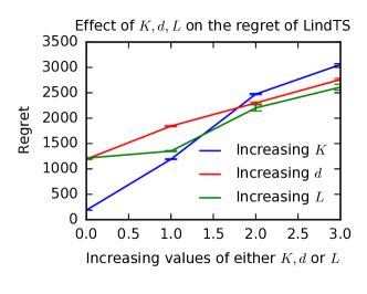
Figure 5: Regret of dTS-LL w.r.t. $K,d,L$.

References

- Abbasi-Yadkori et al. (2011) Abbasi-Yadkori, Y., Pal, D., and Szepesvari, C. Improved algorithms for linear stochastic bandits. In Advances in Neural Information Processing Systems 24, pp. 2312–2320, 2011.
- Abeille & Lazaric (2017) Abeille, M. and Lazaric, A. Linear Thompson sampling revisited. In Proceedings of the 20th International Conference on Artificial Intelligence and Statistics, 2017.
- Agrawal & Goyal (2013a) Agrawal, S. and Goyal, N. Thompson sampling for contextual bandits with linear payoffs. In Proceedings of the 30th International Conference on Machine Learning, pp. 127–135, 2013a.
- Agrawal & Goyal (2013b) Agrawal, S. and Goyal, N. Further optimal regret bounds for thompson sampling. In Proceedings of the Sixteenth International Conference on Artificial Intelligence and Statistics, pp. 99–107, 2013b.
- Agrawal & Goyal (2017) Agrawal, S. and Goyal, N. Near-optimal regret bounds for thompson sampling. Journal of the ACM (JACM), 64(5):1–24, 2017.
- Ajay et al. (2022) Ajay, A., Du, Y., Gupta, A., Tenenbaum, J., Jaakkola, T., and Agrawal, P. Is conditional generative modeling all you need for decision-making? arXiv preprint arXiv:2211.15657, 2022.
- Aouali (2023) Aouali, I. Linear diffusion models meet contextual bandits with large action spaces. In NeurIPS 2023 Foundation Models for Decision Making Workshop, 2023.
- Aouali et al. (2023a) Aouali, I., Brunel, V.-E., Rohde, D., and Korba, A. Exponential smoothing for off-policy learning. In Proceedings of the 40th International Conference on Machine Learning, pp. 984–1017. PMLR, 2023a.
- Aouali et al. (2023b) Aouali, I., Kveton, B., and Katariya, S. Mixed-effect thompson sampling. In International Conference on Artificial Intelligence and Statistics, pp. 2087–2115. PMLR, 2023b.
- Auer et al. (2002) Auer, P., Cesa-Bianchi, N., and Fischer, P. Finite-time analysis of the multiarmed bandit problem. Machine Learning, 47:235–256, 2002.
- Azar et al. (2013) Azar, M. G., Lazaric, A., and Brunskill, E. Sequential transfer in multi-armed bandit with finite set of models. In Advances in Neural Information Processing Systems 26, pp. 2220–2228, 2013.
- Bastani et al. (2019) Bastani, H., Simchi-Levi, D., and Zhu, R. Meta dynamic pricing: Transfer learning across experiments. CoRR, abs/1902.10918, 2019. URL https://arxiv.org/abs/1902.10918.
- Basu et al. (2021) Basu, S., Kveton, B., Zaheer, M., and Szepesvari, C. No regrets for learning the prior in bandits. In Advances in Neural Information Processing Systems 34, 2021.
- Bishop (2006) Bishop, C. M. Pattern Recognition and Machine Learning, volume 4 of Information science and statistics. Springer, 2006.
- Cella et al. (2020) Cella, L., Lazaric, A., and Pontil, M. Meta-learning with stochastic linear bandits. In Proceedings of the 37th International Conference on Machine Learning, 2020.
- Cella et al. (2022) Cella, L., Lounici, K., and Pontil, M. Multi-task representation learning with stochastic linear bandits. arXiv preprint arXiv:2202.10066, 2022.
- Chapelle & Li (2012) Chapelle, O. and Li, L. An empirical evaluation of Thompson sampling. In Advances in Neural Information Processing Systems 24, pp. 2249–2257, 2012.
- Deshmukh et al. (2017) Deshmukh, A. A., Dogan, U., and Scott, C. Multi-task learning for contextual bandits. In Advances in Neural Information Processing Systems 30, pp. 4848–4856, 2017.
- Dhariwal & Nichol (2021) Dhariwal, P. and Nichol, A. Diffusion models beat gans on image synthesis. Advances in neural information processing systems, 34:8780–8794, 2021.
- Filippi et al. (2010) Filippi, S., Cappe, O., Garivier, A., and Szepesvari, C. Parametric bandits: The generalized linear case. In Advances in Neural Information Processing Systems 23, pp. 586–594, 2010.
- Foster et al. (2020) Foster, D. J., Gentile, C., Mohri, M., and Zimmert, J. Adapting to misspecification in contextual bandits. Advances in Neural Information Processing Systems, 33:11478–11489, 2020.
- Gentile et al. (2014) Gentile, C., Li, S., and Zappella, G. Online clustering of bandits. In Proceedings of the 31st International Conference on Machine Learning, pp. 757–765, 2014.
- Gopalan et al. (2014) Gopalan, A., Mannor, S., and Mansour, Y. Thompson sampling for complex online problems. In Proceedings of the 31st International Conference on Machine Learning, pp. 100–108, 2014.
- Gupta et al. (2018) Gupta, S., Chaudhari, S., Mukherjee, S., Joshi, G., and Yagan, O. A unified approach to translate classical bandit algorithms to the structured bandit setting. CoRR, abs/1810.08164, 2018. URL https://arxiv.org/abs/1810.08164.
- Ho et al. (2020) Ho, J., Jain, A., and Abbeel, P. Denoising diffusion probabilistic models. Advances in neural information processing systems, 33:6840–6851, 2020.
- Hong et al. (2020) Hong, J., Kveton, B., Zaheer, M., Chow, Y., Ahmed, A., and Boutilier, C. Latent bandits revisited. In Advances in Neural Information Processing Systems 33, 2020.
- Hong et al. (2022a) Hong, J., Kveton, B., Katariya, S., Zaheer, M., and Ghavamzadeh, M. Deep hierarchy in bandits. In International Conference on Machine Learning, pp. 8833–8851. PMLR, 2022a.
- Hong et al. (2022b) Hong, J., Kveton, B., Zaheer, M., and Ghavamzadeh, M. Hierarchical Bayesian bandits. In Proceedings of the 25th International Conference on Artificial Intelligence and Statistics, 2022b.
- Hsieh et al. (2023) Hsieh, Y.-G., Kasiviswanathan, S. P., Kveton, B., and Blöbaum, P. Thompson sampling with diffusion generative prior. arXiv preprint arXiv:2301.05182, 2023.
- Hu et al. (2021) Hu, J., Chen, X., Jin, C., Li, L., and Wang, L. Near-optimal representation learning for linear bandits and linear rl. In International Conference on Machine Learning, pp. 4349–4358. PMLR, 2021.
- Janner et al. (2022) Janner, M., Du, Y., Tenenbaum, J. B., and Levine, S. Planning with diffusion for flexible behavior synthesis. arXiv preprint arXiv:2205.09991, 2022.
- Kaufmann et al. (2012) Kaufmann, E., Korda, N., and Munos, R. Thompson sampling: An asymptotically optimal finite-time analysis. In International conference on algorithmic learning theory, pp. 199–213. Springer, 2012.
- Koller & Friedman (2009) Koller, D. and Friedman, N. Probabilistic Graphical Models: Principles and Techniques. MIT Press, Cambridge, MA, 2009.
- Korda et al. (2013) Korda, N., Kaufmann, E., and Munos, R. Thompson sampling for 1-dimensional exponential family bandits. Advances in neural information processing systems, 26, 2013.
- Kruschke (2010) Kruschke, J. K. Bayesian data analysis. Wiley Interdisciplinary Reviews: Cognitive Science, 1(5):658–676, 2010.
- Kveton et al. (2020) Kveton, B., Zaheer, M., Szepesvari, C., Li, L., Ghavamzadeh, M., and Boutilier, C. Randomized exploration in generalized linear bandits. In International Conference on Artificial Intelligence and Statistics, pp. 2066–2076. PMLR, 2020.
- Kveton et al. (2021) Kveton, B., Konobeev, M., Zaheer, M., Hsu, C.-W., Mladenov, M., Boutilier, C., and Szepesvari, C. Meta-Thompson sampling. In Proceedings of the 38th International Conference on Machine Learning, 2021.
- Lattimore & Munos (2014) Lattimore, T. and Munos, R. Bounded regret for finite-armed structured bandits. In Advances in Neural Information Processing Systems 27, pp. 550–558, 2014.
- Li et al. (2010) Li, L., Chu, W., Langford, J., and Schapire, R. A contextual-bandit approach to personalized news article recommendation. In Proceedings of the 19th International Conference on World Wide Web, 2010.
- Li et al. (2017) Li, L., Lu, Y., and Zhou, D. Provably optimal algorithms for generalized linear contextual bandits. In Proceedings of the 34th International Conference on Machine Learning, pp. 2071–2080, 2017.
- Lindley & Smith (1972) Lindley, D. and Smith, A. Bayes estimates for the linear model. Journal of the Royal Statistical Society: Series B (Methodological), 34(1):1–18, 1972.
- London & Sandler (2019) London, B. and Sandler, T. Bayesian counterfactual risk minimization. In International Conference on Machine Learning, pp. 4125–4133. PMLR, 2019.
- Lu & Van Roy (2019) Lu, X. and Van Roy, B. Information-theoretic confidence bounds for reinforcement learning. In Advances in Neural Information Processing Systems 32, 2019.
- Maillard & Mannor (2014) Maillard, O.-A. and Mannor, S. Latent bandits. In Proceedings of the 31st International Conference on Machine Learning, pp. 136–144, 2014.
- McCullagh & Nelder (1989) McCullagh, P. and Nelder, J. A. Generalized Linear Models. Chapman & Hall, 1989.
- Peleg et al. (2022) Peleg, A., Pearl, N., and Meirr, R. Metalearning linear bandits by prior update. In Proceedings of the 25th International Conference on Artificial Intelligence and Statistics, 2022.
- Riquelme et al. (2018) Riquelme, C., Tucker, G., and Snoek, J. Deep bayesian bandits showdown: An empirical comparison of bayesian deep networks for thompson sampling. arXiv preprint arXiv:1802.09127, 2018.
- Rombach et al. (2022) Rombach, R., Blattmann, A., Lorenz, D., Esser, P., and Ommer, B. High-resolution image synthesis with latent diffusion models. In Proceedings of the IEEE/CVF conference on computer vision and pattern recognition, pp. 10684–10695, 2022.
- Russo & Van Roy (2014) Russo, D. and Van Roy, B. Learning to optimize via posterior sampling. Mathematics of Operations Research, 39(4):1221–1243, 2014.
- Sakhi et al. (2023) Sakhi, O., Alquier, P., and Chopin, N. Pac-bayesian offline contextual bandits with guarantees. In International Conference on Machine Learning, pp. 29777–29799. PMLR, 2023.
- Scott (2010) Scott, S. A modern bayesian look at the multi‐armed bandit. Applied Stochastic Models in Business and Industry, 26:639 – 658, 2010.
- Simchowitz et al. (2021) Simchowitz, M., Tosh, C., Krishnamurthy, A., Hsu, D., Lykouris, T., Dudik, M., and Schapire, R. Bayesian decision-making under misspecified priors with applications to meta-learning. In Advances in Neural Information Processing Systems 34, 2021.
- Sohl-Dickstein et al. (2015) Sohl-Dickstein, J., Weiss, E., Maheswaranathan, N., and Ganguli, S. Deep unsupervised learning using nonequilibrium thermodynamics. In International conference on machine learning, pp. 2256–2265. PMLR, 2015.
- Wan et al. (2021) Wan, R., Ge, L., and Song, R. Metadata-based multi-task bandits with Bayesian hierarchical models. In Advances in Neural Information Processing Systems 34, 2021.
- Wan et al. (2022) Wan, R., Ge, L., and Song, R. Towards scalable and robust structured bandits: A meta-learning framework. CoRR, abs/2202.13227, 2022. URL https://arxiv.org/abs/2202.13227.
- Wang et al. (2022) Wang, Z., Hunt, J. J., and Zhou, M. Diffusion policies as an expressive policy class for offline reinforcement learning. arXiv preprint arXiv:2208.06193, 2022.
- Weiss (2005) Weiss, N. A Course in Probability. Addison-Wesley, 2005.
- Xu & Zeevi (2020) Xu, Y. and Zeevi, A. Upper counterfactual confidence bounds: a new optimism principle for contextual bandits. arXiv preprint arXiv:2007.07876, 2020.
- Yang et al. (2020) Yang, J., Hu, W., Lee, J. D., and Du, S. S. Impact of representation learning in linear bandits. arXiv preprint arXiv:2010.06531, 2020.
- Yu et al. (2020) Yu, T., Kveton, B., Wen, Z., Zhang, R., and Mengshoel, O. Graphical models meet bandits: A variational Thompson sampling approach. In Proceedings of the 37th International Conference on Machine Learning, 2020.
- Zhu et al. (2022) Zhu, Y., Foster, D. J., Langford, J., and Mineiro, P. Contextual bandits with large action spaces: Made practical. In International Conference on Machine Learning, pp. 27428–27453. PMLR, 2022.