An Étude on the Regularization and Renormalization of Divergences in Primordial Observables

Abstract

Many cosmological observables of interest derive from primordial vacuum fluctuations evolved to late times. These observables represent statistical draws from some underlying quantum or statistical field theoretic framework where infinities arise and require regularization. After subtracting divergences, renormalization conditions must be imposed by measurements or observations at some scale, mindful of scheme and background dependence. We review this process on backgrounds that transition from finite duration inflation to radiation domination, and show how in spite of the ubiquity of scaleless integrals, UV divergences can still be meaningfully extracted from quantities that nominally vanish when dimensionally regularized. In this way, one can contextualize calculations with hard cutoffs, distinguishing between UV and IR scales corresponding to the beginning and end of inflation from UV and IR scales corresponding the unknown completion of the theory and its observables. This distinction has significance as observable quantities cannot depend on the latter although they will certainly depend on the former. One can also explicitly show the scheme independence of the coefficients of UV divergent logarithms. Furthermore, certain IR divergences can be shown to be an artifact of the de Sitter limit and are cured for finite duration inflation. For gravitational wave observables, we stress the need to regularize stress tensors that do not presume a prior scale separation in their construction (as with the standard Isaacson form), deriving an improved stress tensor fit to purpose. We conclude by highlighting the inextricable connection between inferring $N_{\rm eff}$ bounds from vacuum tensor perturbations and the process of background renormalization.

I Introductory remarks

Infinities often arise when computing physical observables in any quantum or statistical field theoretic framework. A well defined prescription to regularize and renormalize these divergences has been developed on flat backgrounds, and a transposition of this formalism to curved backgrounds is also possible, albeit with numerous caveats and subtleties that one must be mindful of depending on the context [3, 4, 5].

Divergences can generically be classed into two categories with distinct physical interpretations. Short distance, or ultra-violet (UV) divergences are unambiguously interpreted as an artifact of admitting arbitrarily high energies or momenta in any given calculational setup as a mathematical idealization. Once these infinities have been appropriately subtracted, causality and locality conspire through decoupling [8, 9] to limit the consequences of this idealization to a handful of relevant and marginal operators in a parametrically controlled derivative expansion (see e.g. [1, 2, 10]).

Long wavelength, or infra-red (IR) divergences on the other hand require additional care in their interpretation, as their implications can range from the harmless to the severe. At the very least, they indicate that one has additional work to do in order to arrive at a physical quantity. For instance, IR divergences often feature in intermediate expressions in theories with gapless excitations, and are rendered benign through cancellations when computing physical observables (as is the case in QED). IR divergences could also be signaling the breakdown of a particular perturbative scheme, which can nevertheless be tamed through resummation, as is the case when one studies thermalization in an out of equilibrium context [12, 13, 14], or in QCD scattering via the factorization properties of its soft and collinear limits [15, 16]. In their most problematic incarnation, IR divergences are a harbinger of the instability of the putative background one is attempting perturbation theory around. Precisely which of the latter two possibilities are signaled by certain IR divergences encountered on de Sitter (dS) or quasi de Sitter backgrounds remains an open question (see e.g. [17, 18, 19, 20, 21, 22, 23, 24, 25, 26, 27, 29, 28, 30, 31]).

In operational terms, a class of IR divergences in cosmology trace to complications that arise on time dependent backgrounds when standard background field quantization methods can no longer be taken for granted. Large quantum corrections to the background could invalidate any purported classical background/fluctuation split, which is a limiting case of the general complication of doing perturbation theory around a time evolving background that must satisfy the tadpole condition at any given order in $\hbar$. Although addressing these issues may seem to necessitate the full regalia of non-equilibrium techniques, notable efforts within the context of stochastic inflation and its background statistical field theory limit can be found in [32, 33, 34, 35, 36, 37, 38, 39, 40, 41, 42, 43, 44, 45, 46, 47, 48, 49, 50, 51, 52, 53], as well as within the dynamical renormalization group and open effective field theory approaches [54, 55, 56].

Nevertheless, in situations where one can presume the validity of background field quantization, dealing with divergences in a variety of cosmological applications is a well understood prescription. So much so, that it is often taken for granted and elided in many practical applications in the literature where the ability to meaningfully extract physically observables quantities is taken as a given once divergences have purportedly been tamed. However, as the adage goes, just because something is infinite, does not mean it is zero. The purpose of this article is to review the details of subtracting and renormalizing divergent quantities on backgrounds that should be of practical interest to all cosmologists – one that transitions from an arbitrary but finite duration of inflation through to a phase of radiation domination. Doing so throws up qualitative differences and novelties relative to the analogous procedure on backgrounds corresponding to a single epoch (whether the inflationary, radiation, or matter dominated backgrounds) that warrants a discussion even for the simplest possible scenario of non-interacting, minimally coupled test scalar fields.

Foremost, we note the ubiquity of scaleless integrals for sufficiently light (though not necessarily massless) fields even when one transitions between epochs at a particular energy scale. Nevertheless, despite the fact that scaleless integrals nominally vanish in mass independent regularization schemes, it is still possible to cleanly separate UV and IR divergent contributions (using techniques borrowed from matching calculations in non-relativistic QCD and QED [2, 59]), and compare these to the contributions one would have calculated in mass dependent regularization schemes, such as through imposing hard cutoffs in physical momenta. This is useful, as UV and IR divergences have distinct physical interpretations – whereas UV divergences are to be subtracted with local counterterms, IR divergences cancel among themselves once physical observables are computed. Moreover, even as one finds the expected scheme dependence for the coefficients of nominal power law divergences, one finds identical coefficients for UV divergent logarithms whether one dimensionally regularizes, point splits, or uses hard cutoffs in physical momenta.

Furthermore, one can demonstrate that certain IR divergences encountered in inflationary cosmology are an artifact of the idealization of a past infinite dS geometry and are absent in computations on backgrounds that transition in and out of inflation, whereas unsurprisingly, UV divergences persist. Specifically, we show how the end of inflation does not regulate UV divergences, but instead parameterizes the coefficients of divergent quantities through the ratio of the scales corresponding to the beginning and end of inflation and must still be subtracted in the prescribed way. The implications of this for vacuum contributions to measurable quantities with blue spectra is discussed, as one must be cautious against including contributions that could be nothing more than the Fourier transform of a UV divergence that is to be subtracted on the way to computing observable quantities.

We conclude with a discussion on following through on renormalizing divergences after having subtracted them in the context of calculations that attempt to compute quantum corrections to a given (tree level) background in some form. In simple terms, it is to be stressed that all physical observations are necessarily of fully dressed quantities, and the putative classical background one performs background field quantization around is only to be viewed as a calculational fiction that serves as bootstrap into computing physical observables. Calculations of quantum corrections tell us nothing of their absolute values. Once renormalization conditions are fixed by measurements at a particular scale, all one can compute is how these quantities change with scale. We discuss the implications of this point for the interpretation of $N_{\rm eff}$ bounds from vacuum tensor perturbations in the early universe, which can be boiled down to attempting to calculate a corrected background (i.e. shifted tadpole condition) from an appropriately derived stress tensor for gravitational waves. A definition of the latter that is fit for the purposes of regularization forces us to work with a form that does not assume a prior (time dependent) scale separation in its definition, as is the case with the commonly used Isaacson form. We retrace the derivation of the stress tensor for gravitational waves and derive an improved version suitable for regularization. We comment in closing how can one in principle compute the stress tensor for gravitational waves in a fully covariant formalism, bypassing entirely the need to compute it via correlation functions through Hadamard regularization techniques.

I.1 Outline and scope

The outline of this article is as follows, we first fix conventions and recap how UV and IR divergences arise in computations of standard cosmological observables, stressing that tracers corresponding to energy densities must be extractable from regularized stress tensors or derivatives of two point functions and their convolutions. For sufficiently light degrees of freedom, we show the ubiquity of scaleless integrals, taking care to address the order of various limits when one looks to extract divergences. Taking a cue from non-relativistic QED and QCD, we then show how to split scaleless integrals into UV and IR contributions that otherwise cancel in dimensional regularization. Focusing only on the UV log-divergent parts, one can make sense of calculations in the literature that impose hard cutoffs in physical momenta, finding identical coefficients for the UV divergent logs no matter the scheme. We then consider the process of regularization on backgrounds that transition in and out of inflation to radiation domination. Although scales corresponding to the beginning and end of inflation can be shown to merely parameterize rather than regulate UV divergences, one finds that nominally IR divergent contributions on a dS background are cured in the examples we consider. In attempting to repeat this process for divergences associated with vacuum tensor perturbations, one immediately encounters the need to work with a form of the stress tensor that does not assume a prior scale separation in its construction if one is to integrate over all momenta in intermediate steps. We derive an improved stress tensor for gravitational waves, highlighting its advantages relative to the Isaacson form for applications to primordial observables, and address the relevance of our observations for extracting various cosmological bounds, before offering our concluding remarks. Various details are deferred to the appendices.

This article is intended as a practical tour for the regularization and renormalization of nominally divergent quantities on backgrounds of cosmological interest using well established techniques, although applied to a context where following through on the details is informative to the point of novelty. For this reason, we focus on the simplest possible applications one could think of given the richness of the problems already encountered there – that of minimally coupled non-interacting test scalar fields, and vacuum tensor perturbations sourced by the background expansion. Moreover, we work in a formalism that should be familiar to most practicing cosmologists: two-point functions, power spectra, and spectral densities, all constructed through the intermediary of mode functions derived on a Friedmann-Robertson-Lemaître-Walker (FRLW) slicing, as opposed to working in a fully covariant formalism (see e.g. [3, 4] and references therein). The reason for this is as practical as it is editorial – although the classic references exert a great deal of effort in the study of the regularization of divergences, they are notably sparse in detail when it comes to the process of following through on renormalization though imposing renormalization conditions, which are typically imposed on observables that convolve Fourier space quantities. In the interests of accessibility for the target audience, full covariance is sacrificed for clarity.

II Preliminaries – regularization of stress tensors and correlation functions

All physical observations consist of some sort of energy or momentum transfer between propagating degrees of freedom and some form of detector or tracer, whether directly or indirectly. Although correlation functions serve as a convenient calculational intermediary between any given (effective) description valid during the primordial epoch and observables at late times, they are not necessarily directly observable by themselves. They can, however, be related to observations at later times by acting upon them with the appropriate derivatives to extract energy and momentum, and subsequently convolving them with transfer functions that encapsulate how they are processed by the intervening cosmological evolution (see e.g. [60] for a review). Correlation functions are typically computed in Fourier space, whereas the observations they relate to are made at some fixed temporal and spatial location and involve the coincident limits of bilinear or higher point functions, necessitating subtraction of UV divergences associated with this limit. Well defined coincident limits also implicitly depend on the IR behavior of correlation functions in that any divergences encountered in the latter must cancel between all contributions in convolution with the transfer function for well defined physical observables in any self-consistent calculational setup. In what follows, we elaborate on the process of extracting and subtracting these divergences as appropriate on backgrounds that transition through different epochs. We first focus upon the divergences associated with vacuum two point correlation functions and the associated energy momentum tensors of scalar fields, after which we shift our attention to gravitational waves. In order to do this, we need to establish some preliminary facts and conventions for the discussion that follows.

The energy momentum tensor for a non-interacting, minimally coupled test scalar field $\phi$ on an FRLW background is given by

$$T^{\mu}_{\leavevmode\nobreak\ \nu}=\partial^{\mu}\phi\partial_{\nu}\phi-\frac{1}{2}\delta^{\mu}_{\nu}\left(g^{\lambda\beta}\partial_{\lambda}\phi\partial_{\beta}\phi+m^{2}\phi^{2}\right),$$ (1)

from which we can extract

$$-T^{0}{}_{0}:=\rho=\frac{\phi^{\prime 2}}{2a^{2}}+\frac{(\nabla\phi)^{2}}{2a^{2}}+\frac{m^{2}}{2}\phi^{2},$$ (2)

where we work in conformal time, and primes denote derivatives with respect to conformal time. The above is a local density that we can rewrite as the coincident limit of a bilinear form as

$$\rho:=\lim_{y\to x}\rho(\tau;x,y),$$ (3)

where

$$\rho(\tau;x,y):=\frac{1}{2a^{2}}\left[\phi^{\prime}(\tau,x)\phi^{\prime}(\tau,y)+\nabla_{x}\phi(\tau,x)\cdot\nabla_{y}\phi(\tau,y)+m^{2}a^{2}\phi(\tau,x)\phi(\tau,y)\right].$$ (4)

Given the Fourier transform convention for the corresponding field operator $\hat{\phi}$

$$\hat{\phi}(\tau,x)=\int\frac{d^{3}k}{(2\pi)^{3}}\hat{\phi}(\tau,k)e^{ik\cdot x},$$ (5)

where the argument distinguishes the field operator in position space from its Fourier component, and the definition

$$\frac{k^{3}}{2\pi^{2}}\langle\hat{\phi}(\tau,k)\hat{\phi}(\tau,k^{\prime})\rangle:=(2\pi)^{3}\delta^{3}(k+k^{\prime})\mathcal{P}_{\phi}(\tau,k),$$ (6)

we can express the two point correlation function as

$$\langle\hat{\phi}(\tau,x)\hat{\phi}(\tau,y)\rangle = \int\frac{d^{3}k}{4\pi}\frac{\mathcal{P}_{\phi}(\tau,k)}{k^{3}}e^{ik\cdot(x-y)},$$

$$= \int\frac{dk}{k}\mathcal{P}_{\phi}(\tau,k)\frac{\sin(kr)}{kr},$$

where we have assumed statistical isotropy to perform the angular integrals, and $r:=|x-y|$, and will work with the adiabatic vacuum associated with a given background in what follows. For inflationary spacetimes, this will be the usual Bunch Davies vacuum state. The coincident limit of Eq. II can be expressed as

$$\langle\hat{\phi}(\tau,x)\hat{\phi}(\tau,x)\rangle=\int_{0}^{\infty}\frac{dk}{k}\mathcal{P}_{\phi}(\tau,k),$$ (8)

and the coincident limit of Eq. 4 can similarly be expressed as

$$\lim_{y\to x}\rho(\tau;x,y)=\frac{1}{2a^{2}}\int_{0}^{\infty}\frac{dk}{k}\left[\left(k^{2}+a^{2}m^{2}\right)\mathcal{P}_{\phi}(\tau,k)+\mathcal{P}_{\phi^{\prime}}(\tau,k)\right],$$ (9)

where we have used the shorthand

$$\frac{k^{3}}{2\pi^{2}}\langle\hat{\phi}^{\prime}(\tau,k)\hat{\phi}^{\prime}(\tau,k^{\prime})\rangle:=(2\pi)^{3}\delta^{3}(k+k^{\prime})\mathcal{P}_{\phi^{\prime}}(\tau,k).$$ (10)

In terms of canonically normalized mode functions $\phi_{k}(\tau)$ of the appropriate adiabatic vacuum, the free field operator admits the expansion

$$\hat{\phi}(\tau,k)=\hat{a}_{k}\phi_{k}(\tau)+\hat{a}^{\dagger}_{-k}\phi_{k}^{*}(\tau),$$ (11)

where $[\hat{a}_{k},\hat{a}^{\dagger}_{-k^{\prime}}]=(2\pi)^{3}\delta^{3}(k+k^{\prime})$, so that

$$\mathcal{P}_{\phi}(\tau,k)=\frac{k^{3}}{2\pi^{2}}|\phi_{k}(\tau)|^{2},$$ (12)

and so that Eq. 9 can be expressed as

$$\lim_{y\to x}\rho(\tau;x,y)=\frac{1}{4\pi^{2}a^{2}}\int_{0}^{\infty}k^{2}\,dk\left[(k^{2}+a^{2}m^{2})|\phi_{k}(\tau)|^{2}+|\phi^{\prime}_{k}(\tau)|^{2}\right].$$ (13)

On a purely dS background, the mode functions for a massless field are given by

$$|\phi_{k}(\tau)|^{2}=\frac{H^{2}}{2k^{3}}(1+k^{2}\tau^{2}),\leavevmode\nobreak\ \leavevmode\nobreak\ \leavevmode\nobreak\ \leavevmode\nobreak\ |\phi^{\prime}_{k}(\tau)|^{2}=\frac{H^{2}}{2k^{3}}k^{4}\tau^{2},$$ (14)

so that the late time power spectrum for a massless test scalar is exactly scale invariant with amplitude determined from the Bunch Davies vacuum as $\mathcal{P}_{\phi}=\left(\frac{H}{2\pi}\right)^{2}$, where $H$ is the Hubble factor that defines the dS background, so that Eq. 8 reduces to

$$\lim_{\tau\to 0}\langle\hat{\phi}(\tau,x)\hat{\phi}(\tau,x)\rangle=\left(\frac{H}{2\pi}\right)^{2}\int_{0}^{\infty}\frac{dk}{k}.$$ (15)

This above is evidently divergent in both the UV and IR. Qualitatively similar divergences are encountered when one constructs the corresponding energy momentum tensor, as we attend to in the next section, warranting a detour on the different approaches one might adopt to regularize expressions like the above where important caveats immediately arise.

II.1 Regularization scheme (in)dependence

Given the absence of any scale in the integrand in Eq. 15, the integral vanishes in mass independent regularization schemes such as dimensional or zeta function regularization (see e.g. the relevant chapters of [1, 2]). One might perhaps be wary of this and imagine instead regulating such an expression by imposing hard cutoffs in both the UV and the IR. However, one is immediately presented with a choice as to precisely how. For instance, [55] adopts cutoffs in terms of physical momenta on the basis that since IR divergences must cancel in all physical processes, the IR scales associated with these must be expressed in terms of physical scales. On the other hand, [61] argues that it is more practical to adopt cutoffs in terms of comoving momenta for IR divergences given that the existence of a pre-inflationary phase ought to serve as a natural regulator where the distinction becomes less relevant (in the sense that it leads to only sub-leading corrections). Although we explicitly demonstrate the nature of a pre-inflationary phase as an IR regulator in subsequent sections, we wish to stress that aside from the expected scheme dependence that will drop out of physical quantities once renormalization conditions are imposed consistently, using hard cutoffs in physical momenta works particularly straightfowardly for matching with the logarithmic UV divergences one can extract from scaleless integrals, and moreover leads to straightforward identification of the requisite counterterms. Simply put, one can arrive at the same expressions for the logarithmic running of physical quantities regardless of regularization scheme with sufficient care, as is to be expected. The fact that UV and IR divergences can be extracted and separated from scaleless integrals may come as a surprise to those used to discarding them, so it behooves us to elaborate on this in detail.

II.2 UV and IR divergences in mass (in)dependent schemes

Reconsider the scaleless integral Eq. 15, which can formally be rewritten as

$$\int_{0}^{\infty}\frac{dk}{k}=\int_{0}^{\infty}\frac{k^{3}dk}{k^{4}}=\frac{1}{2\pi^{2}}\int_{-\infty}^{\infty}\frac{d^{4}k}{k^{4}},$$ (16)

where the formal manipulations that result in the above render this integral to be Euclidean by default. We see that Eq.16 is a specific case of the more general form [2]

$$I_{D}(m^{2})=\int\frac{d^{D}k}{(2\pi)^{D}}\frac{k^{2A}}{(k^{2}+m^{2})^{B}}.$$ (17)

Formally, Eq. 17 evaluates to

$$I_{D}(m^{2})=\frac{\Gamma\left(A+\frac{D}{2}\right)\Gamma\left(B-A-\frac{D}{2}\right)}{(4\pi)^{D/2}\Gamma\left(\frac{D}{2}\right)\Gamma(B)}\left(m^{2}\right)^{A-B+D/2},$$ (18)

which permits analytic continuation to non-integer values of $D$. Re-expressing the two point function Eq. 15 via Eq. 16 as

$$\lim_{\tau\to 0}\langle\hat{\phi}(\tau,x)\hat{\phi}(\tau,x)\rangle=\frac{H^{2}}{8\pi^{4}}\int_{-\infty}^{\infty}\frac{d^{4}k}{k^{4}}=\frac{H^{2}}{8\pi^{4}}\int_{-\infty}^{\infty}d^{4}k\left[\frac{1}{k^{2}(k^{2}+m^{2})}+\frac{m^{2}}{k^{4}(k^{2}+m^{2})}\right],$$ (19)

we see via Eq. 18 that this evaluates in $D=4-\delta$ dimensions to two equal and opposite contributions of the form

$$\pm\frac{H^{2}}{4\pi^{2}}\left[\frac{1}{\delta}-\frac{1}{2}\left(\log\frac{m^{2}}{4\pi\mu^{2}}+\gamma_{E}-1\right)\right],$$ (20)

where $\gamma_{E}$ is the Euler-Mascheroni constant, and $\mu$ is some arbitrary mass scale necessitated by dimensional deformation. The sum of the two contributions can be written as

$$\lim_{\tau\to 0}\langle\hat{\phi}(\tau,x)\hat{\phi}(\tau,x)\rangle=\left(\frac{H}{2\pi}\right)^{2}\left[\frac{1}{\delta_{\rm UV}}-\frac{1}{\delta_{\rm IR}}+\log\frac{\mu_{\rm UV}}{\mu_{\rm IR}}\right],$$ (21)

where we have artificially given a separate label to the dimensional deformation parameters $\delta$ and $\mu$ from the two terms to distinguish the UV and IR divergent contributions in Eq. 19, illustrating the anatomy of how dimensional regularization works in canceling two separately divergent contributions by default.

It is informative to compare this result with the outcome of imposing hard cutoffs. Whether we chose to do so in Eq. 15 in terms of physical momenta (where $\Lambda_{\rm UV/IR}=a\,k_{\rm UV/IR}$) or in terms of comoving momenta (where $\Lambda_{\rm UV/IR}=k_{\rm UV/IR}$) is immaterial in the context of logarithmic divergences which only sees ratios of these scales:

$$\lim_{\tau\to 0}\langle\hat{\phi}(\tau,x)\hat{\phi}(\tau,x)\rangle=\left(\frac{H}{2\pi}\right)^{2}\log\left(\frac{k_{\rm UV}}{k_{\rm{IR}}}\right).$$ (22)

From this, we see that in spite of the fact that scaleless integrals vanish under dimensional regularization, factorizing them into a sum of scaleful integrals allows one to match the coefficients of the UV divergent logarithms in Eq. 21 with those in Eq. 22 obtained by imposing hard cutoffs in physical momenta. As we show in subsequent sections, this will also be true no matter the background.

III Non-interacting test scalar fields

In this section, we examine divergences in the two point correlation function and energy momentum tensor for non-interacting, minimally coupled massless test scalar fields on dS and quasi dS backgrounds, as well as that for sufficiently light massive scalar fields on a dS background. All divergent integrals turn out to be scaleless, a feature that persists even when one considers a background that transitions from a pre-inflationary epoch through to inflation and exiting to a terminal phase of radiation domination. Nevertheless, one can extract UV divergences via the techniques elaborated in section II.2 and compare with what one would have obtained with a hard cutoff in physical momenta, recovering identical coefficients for the logarithmic divergences.

III.1 Divergences – (quasi) dS backgrounds

On backgrounds that deviate from dS, one has to be careful to factor in the difference in the scale factor from the pure dS form of $a(\tau)=-1/(H\tau)$. For constant but non-zero $\epsilon:=-\dot{H}/H^{2}$, as is the case during power law inflation for instance, one has $a(\tau)=1/[-\tau H_{0}]^{\nu-1/2}$, where $\nu=\frac{3-\epsilon}{2(1-\epsilon)}$ (and where the integration constant $H_{0}$ corresponds to the value of $H$ at $t=0$ in cosmological time – cf. [60]). The net result for the coincident limit of the two point function for a massless scalar field on a background corresponding to constant $\epsilon$ is given by

$$\lim_{\tau\to 0}\langle\hat{\phi}(\tau,x)\hat{\phi}(\tau,x)\rangle=\left(\frac{H_{0}}{2\pi}\right)^{2}\frac{\Gamma^{2}(\nu)}{\pi}2^{2\nu-1}\int_{0}^{\infty}\frac{dk}{k}\left(\frac{k}{H_{0}}\right)^{3-2\nu}\left[1+\frac{k^{2}\tau^{2}}{2(\nu-1)}+...\right],$$ (23)

or more generally,

$$\lim_{\tau\to 0}\langle\hat{\phi}(\tau,x)\hat{\phi}(\tau,x)\rangle\sim\left(\frac{H_{0}}{2\pi}\right)^{2}\int_{0}^{\infty}\frac{dk}{k}\left(\frac{k}{H_{0}}\right)^{n_{s}-1}\left[1+\left(\frac{k}{aH_{0}}\right)^{2}\frac{a^{n_{s}-1}}{2-n_{s}}+...\right]$$ (24)

where the ellipses denote terms that vanish in the $\tau\to 0$ limit and the $\sim$ indicates a numerical pre-factor that is close to unity for $n_{s}-1\approx 1$ (and tends to it in the dS limit). In the dS limit, we find the relatively simple expression

$$\lim_{\tau\to 0}\langle\hat{\phi}(\tau,x)\hat{\phi}(\tau,x)\rangle=\left(\frac{H_{0}}{2\pi}\right)^{2}\int_{0}^{\infty}\frac{dk}{k}\left[1+\left(\frac{k}{aH_{0}}\right)^{2}\right],$$ (25)

which supplements Eq. 15 with a sub-leading correction in the late time limit, notable relative to the analogous expression on quasi dS Eq. 24 in that is Eq. 25 exact for all times. The scaleless nature of Eq. 24 implies that it vanishes when regularized in any mass independent scheme. Instead, one might contemplate imposing a hard UV or IR cutoff in physical momenta by setting $k_{\rm UV/IR}=a\Lambda_{\rm UV/IR}$, and subtracting the UV divergence with the necessary counterterm. Doing so for the expression Eq. 25, one finds (see e.g. [55])

$$\lim_{\tau\to 0}\langle\hat{\phi}(\tau,x)\hat{\phi}(\tau,x)\rangle = \left(\frac{H_{0}}{2\pi}\right)^{2}\left\{\int_{a\Lambda_{\rm IR}}^{a\Lambda_{\rm UV}}\frac{dk}{k}\left[1+\left(\frac{k}{aH_{0}}\right)^{2}\right]-\int_{a\mu}^{a\Lambda_{\rm UV}}\frac{dk}{k}\left[1+\left(\frac{k}{aH_{0}}\right)^{2}\right]\right\},$$

$$= \left(\frac{H_{0}}{2\pi}\right)^{2}\left\{\log\left(\frac{\mu}{\Lambda_{\rm IR}}\right)+\frac{1}{2H_{0}^{2}}\left(\mu^{2}-\Lambda_{\rm IR}^{2}\right)\right\},\leavevmode\nobreak\ \leavevmode\nobreak\ \leavevmode\nobreak\ \leavevmode\nobreak\ \leavevmode\nobreak\ \leavevmode\nobreak\ \leavevmode\nobreak\ \leavevmode\nobreak\ \leavevmode\nobreak\ \leavevmode\nobreak\ \leavevmode\nobreak\ \leavevmode\nobreak\ \leavevmode\nobreak\ \leavevmode\nobreak\ \leavevmode\nobreak\ \leavevmode\nobreak\ \leavevmode\nobreak\ \leavevmode\nobreak\ \leavevmode\nobreak\ \leavevmode\nobreak\ (n_{s}=1)$$

where $\mu$ is some arbitrary renormalization scale. We note that the counterterm that subtracts the UV divergence in Eq. III.1 is given by

$${\rm c.t.}=\left(\frac{H_{0}}{2\pi}\right)^{2}\left\{\log\left(\frac{\mu}{\Lambda_{\rm UV}}\right)+\frac{1}{2H_{0}^{2}}\left(\mu^{2}-\Lambda_{\rm UV}^{2}\right)\right\},$$ (27)

corresponding to a scheme dependent renormalization of the cosmological constant. That these expressions are independent of time is a consequence of having imposed a physical cutoff on a dS invariant background. The remaining IR divergence is indicative of the fact that we have not yet arrived at something that can be processed into an observable quantity. It could end up being canceled by other contributions when we compute a well defined observable, or it could herald the need for resummation in which case it will also eventually get canceled. It could also indicate that the background we are attempting quantization around is not what it seems [66], and additional physical inputs are required in order to proceed. As we will show explicitly in what follows, were we to abandon the assumption that inflation was past dS eternal, then all IR divergences cancel among themselves and are in effect regulated by the scale corresponding to the beginning of inflation.

It is informative to compare what we would have obtained if we had dimensionally regularized Eq. 25 instead. We first note that the scaleless nature of the integral permits us to change variables to $q:=k/(aH_{0})$ for any fixed time. Hence the integral we need to evaluate can be factorized as in Eq. 19 as:

$$\frac{H^{2}_{0}}{8\pi^{4}}\int_{-\infty}^{\infty}\frac{d^{4}q}{q^{4}}(1+q^{2}) = \frac{H_{0}^{2}}{8\pi^{4}}\int_{-\infty}^{\infty}d^{4}q\left[\frac{1}{(q^{2}+\widetilde{m}^{2})}+\frac{1+\widetilde{m}^{2}}{q^{2}(q^{2}+\widetilde{m}^{2})}+\frac{\widetilde{m}^{2}}{q^{4}(q^{2}+\widetilde{m}^{2})}\right]$$ (28)

where $\widetilde{m}:=\mu/H_{0}$ is some auxiliary dimensionless mass scale. The first and second terms above are power law and log divergent in the UV, respectively, whereas the third term is IR divergent. The UV divergences must of course, be subtracted by an appropriate counterterm. One finds after cancellations between the contributions from the first and second terms of Eq. 28, a remaining UV divergence

$${\rm c.t.}=\left(\frac{H_{0}}{2\pi}\right)^{2}\left\{\log\left(\frac{\mu}{H_{0}}\right)-\frac{1}{\delta_{\rm UV}}+\frac{1}{2}\left(\gamma_{E}-1-\log 4\pi\right)\right\},$$ (29)

which is to be compared to Eq. 27.

The situation for quasi dS is more complicated if one were to regularize it in a mass dependent scheme, as is evident from Eq. 24. Nevertheless, it is still worth elaborating upon provided we simplify matters by further specifying that the background corresponds to that of eternal power-law inflation, defined by a constant but non-zero $\epsilon$, so that $n_{s}-1=-2\epsilon-2\epsilon^{2}+...$. We will address the more realistic case of finite duration inflation next. One finds from inspection of the integrand of Eq. 24:

$$\int_{0}^{\infty}\frac{dk}{k}\left(\frac{k}{H_{0}}\right)^{n_{s}-1}\left[1+\left(\frac{k}{aH_{0}}\right)^{2}\frac{a^{n_{s}-1}}{2-n_{s}}\right]$$ (30)

that for $n_{s}-1<0$, an IR divergent contribution results from the first term:

$$\int_{0}^{\infty}\frac{dk}{k}\left(\frac{k}{H_{0}}\right)^{n_{s}-1}=\frac{1}{|n_{s}-1|}\left(\frac{a\Lambda_{\rm IR}}{H_{0}}\right)^{n_{s}-1},$$ (31)

and a UV divergent contribution results from the second

$$\int_{0}^{\infty}\frac{dk}{k}\left(\frac{k}{aH_{0}}\right)^{n_{s}+1}\frac{a^{2(n_{s}-1)}}{2-n_{s}}=\frac{a^{2(n_{s}-1)}}{(2-n_{s})(n_{s}-1)}\left(\frac{\Lambda_{\rm UV}}{H_{0}}\right)^{n_{s}+1}.$$ (32)

The interpretation of the IR divergences is as discussed above. The UV divergence must be subtracted with a local counterterm if we are to obtain physically meaningful quantities, and is given by

$${\rm c.t.}=\lim_{\tau\to 0}\left(\frac{H_{0}}{2\pi}\right)^{2}\frac{a^{2(n_{s}-1)}}{(2-n_{s})(n_{s}-1)}\left[\left(\frac{\mu}{H_{0}}\right)^{n_{s}+1}-\left(\frac{\Lambda_{\rm UV}}{H_{0}}\right)^{n_{s}+1}\right],$$ (33)

where again $\mu$ is some renormalization scale. We first note that the required counterterm is time dependent, which should not come as a surprise given that the background is no longer maximally symmetric. It behooves us to elaborate on the specific form of the local counterterm that could possibly have this particular time dependence. Noting that on the specified power law inflating background, $\dot{H},H^{2}\sim a^{n_{s}-1}$, so that curvature squared invariants evaluated on this background have the required secular dependence. That is, Eq. 33 derives from

$${\rm c.t.}\subset\int d^{4}x\sqrt{-g}\left[c_{1}(\mu)R^{2}+c_{2}(\mu)R_{\mu\nu}R^{\mu\nu}\right],$$ (34)

which are the usual leading curvature squared counterterms encountered in the effective field theory treatment of gravity [67, 68, 69, 70]. In the limit that $\epsilon\to 0$, so that $n_{s}\to 1^{-}$, the counterterm Eq. 33 simplifies to

$${\rm c.t.}=\lim_{\epsilon\to 0}\frac{a^{-4\epsilon}\Lambda^{2}_{\rm UV}}{4\pi^{2}}\left\{\frac{1}{2\epsilon}-\log\frac{\Lambda_{\rm UV}}{H_{0}}+...\right\},$$ (35)

where given that $\Lambda_{\rm UV}\gg\mu$, we have neglected the sub-leading dependence on $\mu$.

As before, we can retrace the same computation using dimensional regularization. We first consider the separate contributions to the integrand Eq. 30. The IR divergent contribution Eq. 31 can be re-expressed as

$$\int_{0}^{\infty}\frac{dk}{k}\left(\frac{k}{H_{0}}\right)^{n_{s}-1}=\frac{1}{2\pi^{2}}\int_{-\infty}^{\infty}\frac{d^{4}q}{q^{4}}q^{n_{\rm s}-1}=\frac{1}{2\pi^{2}}\int_{-\infty}^{\infty}d^{4}q\left[\frac{q^{n_{\rm s}-1}}{q^{2}(q^{2}+\widetilde{m}^{2})}+\frac{\widetilde{m}^{2}q^{n_{s}-1}}{q^{4}(q^{2}+\widetilde{m}^{2})}\right],$$ (36)

where we have switched to the dimensionless variable $q:=k/H_{0}$, and similarly for $\widetilde{m}:=\mu_{\rm IR}/H_{0}$. The presence of the non-integer exponents eliminates the $\delta$ poles, and one finds equal and opposite contributions from the two constituent integrals, with the nominally IR divergent contribution coming from the second term of the form

$$\lim_{n_{s}\to 1^{-}}-\left\{\frac{1}{n_{s}-1}+\log\frac{\mu_{\rm IR}}{H_{0}}+(n_{\rm s}-1)\left(\frac{\pi^{2}}{24}+\frac{1}{2}\log^{2}\frac{\mu_{\rm IR}}{H_{0}}\right)+...\right\},$$ (37)

whose interpretation is as in the previous examples. Turning to the UV divergent term Eq. 32:

$$\frac{a^{2(n_{s}-1)}}{2-n_{s}}\int_{0}^{\infty}\frac{dk}{k}\left(\frac{k}{aH_{0}}\right)^{n_{s}+1},$$ (38)

we see that we can again factor the scaleless integrand into the sum of two terms as

$$\int_{0}^{\infty}\frac{dk}{k}\left(\frac{k}{aH_{0}}\right)^{n_{s}+1}=\frac{1}{2\pi^{2}}\int_{-\infty}^{\infty}\frac{d^{4}q}{q^{4}}q^{n_{\rm s}+1}=\frac{1}{2\pi^{2}}\int_{-\infty}^{\infty}d^{4}q\left[\frac{q^{n_{\rm s}+1}}{q^{2}(q^{2}+\widetilde{m}^{2})}+\frac{\widetilde{m}^{2}q^{n_{s}+1}}{q^{4}(q^{2}+\widetilde{m}^{2})}\right],$$ (39)

where just as we did on dS space, we work with dimensionless variables $q:=k/aH_{0}$ and $\widetilde{m}:=\mu/H_{0}$. The first term above is UV divergent, and necessitates the counterterm

$${\rm c.t.} = \lim_{\epsilon\to 0}-\frac{a^{2(n_{s}-1)}}{2-n_{s}}\left(\frac{H_{0}}{2\pi}\right)^{2}\frac{\mu^{2}}{H_{0}^{2}}\left\{\frac{1}{n_{s}-1}+\log\frac{\mu}{H_{0}}\right\}$$

$$= \lim_{\epsilon\to 0}\frac{a^{-4\epsilon}\mu^{2}}{4\pi^{2}}\left\{\frac{1}{2\epsilon}-\log\frac{\mu}{H_{0}}+...\right\}$$

which is to be compared to Eq. 35.

The generalization to massive fields is straightforward on dS backgrounds, where analytic expressions for the mode functions can be obtained:

$$|\phi_{k}(\tau)|^{2}=\frac{\pi}{4}H_{0}^{2}(-\tau)^{3}|H^{(1)}_{\nu_{m}}(-k\tau)|^{2},$$ (41)

where

$$\nu^{2}_{m}:=\frac{9}{4}-\frac{m^{2}}{H_{0}^{2}},$$ (42)

and where $H^{(1)}_{\nu_{m}}$ is the corresponding Hankel function with degree $\nu_{m}$. Presuming $0<m^{2}\leq 9H_{0}^{2}/4$ so that $\nu_{m}$ is still real, the coincident limit of the two point function at late times can then be computed as

$$\lim_{\tau\to 0}\langle\hat{\phi}(\tau,x)\hat{\phi}(\tau,x)\rangle=\frac{H_{0}^{2}}{8\pi^{3}}2^{2\nu_{m}}\Gamma^{2}(\nu_{m})\int_{0}^{\infty}\frac{dk}{k}\left[\left(\frac{k}{aH_{0}}\right)^{3-2\nu_{m}}+\frac{1}{2\left(\nu_{m}-1\right)}\left(\frac{k}{aH_{0}}\right)^{5-2\nu_{m}}\right].$$ (43)

It is notable that in spite of the presence of the additional mass scale $m$, the integral remains scaleless. Here also, we can make the change of variable to $q=k/(aH)$, so that the above can be recast as

$$\lim_{\tau\to 0}\langle\hat{\phi}(\tau,x)\hat{\phi}(\tau,x)\rangle = \frac{H_{0}^{2}}{16\pi^{5}}2^{2\nu_{m}}\Gamma^{2}(\nu_{m})\int_{-\infty}^{\infty}\frac{d^{4}q}{q^{4}}q^{3-2\nu_{m}}\left[1+\frac{q^{2}}{2(\nu_{m}-1)}\right],$$ (44)

where the first thing to note is that the IR divergence encountered for a non-interacting massless scalar on dS is eliminated given that $\nu_{m}<3/2$. Proceeding exactly as before, we can compare the UV divergence obtained from imposing a hard cutoff in physical momenta to that obtained by factorizing the scaleless integral in dimensional regularization. In the limit $m^{2}/H_{0}^{2}\ll 1$, one finds that the required counterterms are given by

$${\rm c.t.}=\frac{H_{0}^{2}}{8\pi^{2}}\frac{2^{2\nu_{m}}\Gamma^{2}(\nu_{m})}{\pi}\left[\frac{3H_{0}^{2}}{m^{2}}+\log\frac{\Lambda_{\rm UV}}{H_{0}}+...\right]\leavevmode\nobreak\ \leavevmode\nobreak\ {(\rm physical\leavevmode\nobreak\ cutoff)}$$ (45)

and

$${\rm c.t.}=\frac{H_{0}^{2}}{8\pi^{2}}\frac{2^{2\nu_{m}}\Gamma^{2}(\nu_{m})}{\pi}\left[\frac{3H_{0}^{2}}{m^{2}}+\log\frac{\mu}{H_{0}}+...\right]\leavevmode\nobreak\ \leavevmode\nobreak\ \leavevmode\nobreak\ \leavevmode\nobreak\ \leavevmode\nobreak\ \leavevmode\nobreak\ \leavevmode\nobreak\ \leavevmode\nobreak\ \leavevmode\nobreak\ {(\rm dim\leavevmode\nobreak\ reg)}$$ (46)

where again, one takes the limit $\delta\to 0$ to regularize the integrals before taking the limit $m^{2}/H_{0}^{2}\to 0$. In both cases, the required counterterm corresponds to a renormalization of the cosmological constant.

Having labored over the details of regularizing and renormalizing divergences for the two point function of test scalar fields, repeating the exercise for the associated stress tensor may seem a straightforward extension. However, we immediately encounter a difficulty: it is not always possible to construct a counterterm that subtracts the UV divergences encountered from background geometric invariants if the regularization scheme itself does not respect this symmetry. This is not to a concern to be casually dismissed, as persisting with this regularization scheme could lead us to the erroneous conclusion that the background we attempted to quantize around is transmuting into something else under renormalization if not worked through to the end. It is here that dimensional and related zeta function regularization techniques distinguish themselves in theories with general covariance, as they effortlessly preserve the symmetries of the background even if the precise mechanism by which this occurs can seem non-trivial. For this reason, it is worth explicitly tracing through this process in detail.

Consider a minimally coupled non-interacting test scalar field on dS space in the Bunch Davies vacuum. The rotational invariance of the vacuum state allow us to write the non-vanishing components as

$$\rho=\frac{1}{4\pi^{2}a^{2}}\int_{0}^{\infty}k^{2}\,dk\left[\left(k^{2}+a^{2}m^{2}\right)|\phi_{k}(\tau)|^{2}+|\phi^{\prime}_{k}(\tau)|^{2}\right],$$ (47)

and

$$p=\frac{1}{4\pi^{2}a^{2}}\int_{0}^{\infty}k^{2}\,dk\left[-\left(\frac{k^{2}}{3}+a^{2}m^{2}\right)|\phi_{k}(\tau)|^{2}+|\phi^{\prime}_{k}(\tau)|^{2}\right],$$ (48)

with all other components of the energy momentum tensor vanishing. From the asymptotic forms of Eq. 41, one can infer that both integrals are UV divergent. The energy density in the massless limit is straightforwardly computed via Eq. 14, and found to be

$$\rho=\frac{H^{4}}{8\pi^{2}}\int^{\infty}_{0}\frac{dk}{k}\left[\left(\frac{k}{aH}\right)^{2}+2\left(\frac{k}{aH}\right)^{4}\right],$$ (49)

and the corresponding pressure is found to be

$$p=\frac{H^{4}}{8\pi^{2}}\int^{\infty}_{0}\frac{dk}{k}\left[-\frac{1}{3}\left(\frac{k}{aH}\right)^{2}+2\left(\frac{k}{aH}\right)^{4}\right],$$ (50)

Although one can regularize both components through imposing physical cutoffs, one is immediately confronted by the fact that the required counterterm for the leading divergences will not be proportional to the metric nor the Ricci tensor on the presumed dS background (which would correspond either to renormalizations of the cosmological and Newton’s constants). This is not the case when one implements dimensional regularization, which may seem rather non-trivial considering the forms that Eqs. 47 and 48 take. Although a fully covariant formalism to regularize stress tensors using mass independent schemes is the industry standard (as elaborated upon in [3, 4]), it is nevertheless informative to trace through this process for the foliation specific forms Eq. 47 and 48, as we do in Appendix A.

The important lesson to draw from this is that regularizing the divergence of just one particular component of the stress tensor (such as the energy density) is not enough. Computing physically sensible quantities derived from the energy momentum tensor in a reliable manner necessitates constructing the appropriate counterterm, without which renormalization conditions cannot be consistently imposed. If the required counterterm cannot be constructed from background quantities in a particular regularization scheme, then all subsequent conclusions will necessarily be scheme dependent, and therefore unphysical. For this reason, regularization schemes that preserve general covariance such as dimensional or zeta function regularization are preferred in this context. In spite of this caveat, however, one can still be forgiven for using hard cutoffs in physical momenta when restricted to calculating logarithmic divergences, as one can show the result to be identical to what would have been obtained in a mass independent scheme. We will return to this point in regards the regularization of the stress tensor for gravitational waves in the next section.

III.2 Divergences – scalar fields and finite duration inflation

Having acquainted ourselves with the basics of regularizing and renormalizing divergences for familiar quantities, one would like to generalize this to backgrounds that realistically model the universe we inhabit. In particular, one might wonder if the fact that we only obtained scaleless integrals in the previous subsections is an artifact of considering the unrealistic scenario of infinite duration inflation. We show that this situation persists even when we consider a cosmology that transitions between different epochs.

In order for inflation to have finite duration by definition, we must be considering an epoch before and after inflation, which we choose to be radiation domination in both cases. We consider the scale factor to evolve as

$$a(\tau) = a_{\rm R}\left(2-\frac{\tau}{\tau_{\rm I}}\right)e^{-\mathcal{N}_{\rm tot}}\leavevmode\nobreak\ \leavevmode\nobreak\ \leavevmode\nobreak\ \leavevmode\nobreak\ \tau<\tau_{\rm I}$$

$$= a_{\rm R}\left(\frac{\tau_{\rm I}}{\tau}\right)e^{-\mathcal{N}_{\rm tot}}\leavevmode\nobreak\ \leavevmode\nobreak\ \leavevmode\nobreak\ \leavevmode\nobreak\ \tau_{\rm I}<\tau<\tau_{\rm R}$$

$$= a_{\rm R}\left(2-\frac{\tau}{\tau_{\rm R}}\right)\leavevmode\nobreak\ \leavevmode\nobreak\ \leavevmode\nobreak\ \leavevmode\nobreak\ \leavevmode\nobreak\ \leavevmode\nobreak\ \tau_{\rm R}<\tau$$

where $a_{\rm R}$ is the scale factor at reheating, and $\tau_{\rm I}$ and $\tau_{\rm R}$ correspond to the (negative) conformal time at the start and end of inflation respectively, and

$$\mathcal{N}_{\rm tot}=\log(a_{\rm R}/a_{\rm I})=\log(\tau_{\rm I}/\tau_{\rm R})$$ (52)

is the total amount e-folds of inflation. The domain of $\tau$ is $(-\infty,\infty)$ with inflation occurring during negative conformal time. With these definitions, the Hubble rate during inflation is given by

$$H=-\frac{1}{a_{\rm R}\tau_{\rm R}}.$$ (53)

In what follows, we keep the normalization $a_{\rm R}$ arbitrary, although one can readily set $a_{\rm R}\equiv 1$ for convenience in what follows. Here again, we focus on a massless, minimally coupled non-interacting scalar field for illustrative purposes. The mode functions during the terminal stage of radiation domination can be rewritten for the purposes of a matching to the end of inflation as

$$\phi^{\rm RD}_{k} = \frac{1}{a}\frac{1}{\sqrt{2k}}\left[\alpha_{k}^{\rm R}e^{-ik\tau_{\rm R}\left(2-\frac{a}{a_{\rm R}}\right)}+\beta_{k}^{\rm R}e^{ik\tau_{\rm R}\left(2-\frac{a}{a_{\rm R}}\right)}\right]$$ (54)

$$\phi^{\prime\rm RD}_{k} = \frac{a_{\rm R}}{a^{2}\tau_{\rm R}}\frac{1}{\sqrt{2k}}\left[\alpha_{k}^{\rm R}e^{-ik\tau_{\rm R}\left(2-\frac{a}{a_{\rm R}}\right)}\left(1-ik\tau_{\rm R}\frac{a}{a_{\rm R}}\right)+\beta_{k}^{\rm R}e^{ik\tau_{\rm R}\left(2-\frac{a}{a_{\rm R}}\right)}\left(1+ik\tau_{\rm R}\frac{a}{a_{\rm R}}\right)\right].$$

The mode functions during inflation are given by

$$\phi_{k}^{\rm I} = \frac{H}{\sqrt{2k^{3}}}\left[\alpha_{k}^{\rm I}e^{i\frac{k}{aH}}\left(1-\frac{ik}{aH}\right)+\beta_{k}^{\rm I}e^{-i\frac{k}{aH}}\left(1+\frac{ik}{aH}\right)\right]$$ (55)

$$\phi^{\prime\rm I}_{k} = -\frac{H}{\sqrt{2k^{3}}}\left[\alpha_{k}^{\rm I}e^{i\frac{k}{aH}}\frac{k^{2}}{aH}+\beta_{k}^{\rm I}e^{-i\frac{k}{aH}}\frac{k^{2}}{aH}\right],$$

where the presence of non-trivial Bogoliubov coefficients come from having matched to a radiation dominated pre-inflationary phase initiated in the adiabatic vacuum, where the mode functions are given by

$$\phi^{\rm PI}_{k} = \frac{1}{a}\frac{1}{\sqrt{2k}}e^{-ik\tau_{\rm I}\left(2-\frac{a}{a_{\rm R}}e^{\mathcal{N}_{\rm tot}}\right)}$$ (56)

$$\phi^{\prime\rm PI}_{k} = -\frac{1}{a^{2}\sqrt{2k}}\frac{a_{\rm I}}{\tau_{\rm I}}e^{-ik\tau_{\rm I}\left(2-\frac{a}{a_{\rm R}}e^{\mathcal{N}_{\rm tot}}\right)}\left(-1+ik\tau_{\rm I}\frac{a}{a_{\rm I}}\right).$$

One first obtains $\alpha^{\rm I}_{k}$ and $\beta_{k}^{\rm I}$ by matching to the pre-inflationary radiation dominated epoch, so that

$$\alpha_{k}^{\rm I} = \left(i-i\frac{a_{\rm I}^{2}H^{2}}{2k^{2}}+\frac{a_{\rm I}H}{k}\right)$$ (57)

$$\noindent\beta_{k}^{\rm I} = i\frac{a_{\rm I}^{2}H^{2}}{2k^{2}}e^{2i\frac{k}{a_{\rm I}H}}.$$

Similarly, after the matching between inflation and radiation dominated era, one finds that $\alpha^{\rm R}_{k}$ and $\beta_{k}^{\rm R}$ are given by

$$\alpha_{k}^{\rm R} = \alpha_{k}^{\rm I}\left(-i+\frac{a_{\rm R}H}{k}+i\frac{a_{\rm R}^{2}H^{2}}{2k^{2}}\right)+i\beta_{k}^{\rm I}\frac{a_{\rm R}^{2}H^{2}}{2k^{2}}e^{-2i\frac{k}{a_{\rm R}H}}$$

$$\beta_{k}^{\rm R} = -i\alpha_{k}^{\rm I}\frac{a_{\rm R}^{2}H^{2}}{2k^{2}}e^{2i\frac{k}{a_{\rm R}H}}+\beta_{k}^{\rm I}\left(i+\frac{a_{\rm R}H}{k}-i\frac{a_{\rm R}^{2}H^{2}}{2k^{2}}\right).$$ (58)

We now use these results to find expressions for the coincident limits of the two point function and $\rho$ during the terminal stage of radiation domination. The two point correlation function coincidence limit can be expressed as

$$\lim_{x\to y}\langle\hat{\phi}(\tau,x)\hat{\phi}(\tau,y)\rangle = \frac{1}{2\pi^{2}a^{2}}\int_{0}^{\infty}\frac{dk}{k}\>\frac{k^{2}}{2}\left[1+2|\beta_{k}^{\rm R}|^{2}+\alpha^{\rm R}_{k}\beta^{\rm R*}_{k}e^{\frac{2ik}{a_{\rm R}H}\left(2-\frac{a}{a_{\rm R}}\right)}+\alpha^{\rm R*}_{k}\beta^{\rm R}_{k}e^{-\frac{2ik}{a_{\rm R}H}\left(2-\frac{a}{a_{\rm R}}\right)}\right]$$ (59)

$$= \frac{1}{2\pi^{2}a^{2}}\int_{0}^{\infty}\frac{dk}{k}\>\frac{k^{2}}{2}\left[1+2|\beta_{k}^{\rm R}|_{\rm power}^{2}+\{{\rm osc}\}\right]$$

where the first line has used $|\alpha_{k}^{\rm I}|^{2}-|\beta_{k}^{\rm I}|^{2}=|\alpha_{k}^{\rm R}|^{2}-|\beta_{k}^{\rm R}|^{2}=1$, and the second line splits the integrand into strictly power law contributions and oscillatory contributions. From Eqs. 57 and III.2, we find that

$$|\beta^{\rm R}_{k}|_{\rm power}^{2}=\frac{a_{\rm R}^{4}H^{4}+a_{\rm I}^{4}H^{4}}{4k^{4}}+\frac{a_{\rm I}^{4}a_{\rm R}^{4}H^{8}}{8k^{8}},$$ (60)

which nominally appears to have aggravated the IR divergence of the two point function. However, as we demonstrate in Appendix B, although the oscillatory terms can indeed be neglected for the purposes of extracting UV divergences, the oscillations freeze in the IR and exactly cancel the contributions from $|\beta^{\rm R}_{k}|_{\rm power}^{2}$. Specifically, one finds that

$$\lim_{k\to 0}\{{\rm osc}\}=-\frac{a_{\rm R}^{4}H^{4}+a_{\rm I}^{4}H^{4}}{2k^{4}}-\frac{a_{\rm I}^{4}a_{\rm R}^{4}H^{8}}{4k^{8}}-1+\frac{(3a_{\rm I}^{3}a_{\rm R}+2a(a_{\rm R}^{3}-a_{\rm I}^{3}))^{2}}{9a_{\rm I}^{2}a_{\rm R}^{6}},$$ (61)

which cancels the contributions from $1+2|\beta^{\rm R}_{k}|_{\rm power}^{2}$, leaving only the UV divergence resulting from the final term of Eq. 61 to reckon with:

$$\lim_{x\to y}\langle\hat{\phi}(\tau,x)\hat{\phi}(\tau,y)\rangle_{\rm div} = e^{-4N_{\rm tot}}\left(3+\frac{2a}{a_{\rm R}}\left[e^{3\mathcal{N}_{\rm tot}-1}\right]\right)^{2}\frac{1}{36\pi^{2}a^{2}}\int_{0}^{\infty}dk\>k,$$ (62)

where as before, $e^{-\mathcal{N}_{\rm tot}}=a_{\rm I}/a_{\rm R}$. Two things are to be immediately noted. Firstly, that the physical UV and IR scales $k_{\rm IR/UV}=a_{\rm I/R}H$ associated with the beginning and end of inflation do not by themselves regulate the UV divergences. Instead, they merely parameterize the divergence through their ratio $k_{\rm IR}/k_{\rm UV}=e^{-\mathcal{N}_{\rm tot}}$ in the pre-factor above. Furthermore, the pre-factor itself diverges as $\mathcal{N}_{\rm tot}\to\infty$, indicative of the restoration of the pathologies of a past infinite dS space in that limit, where moreover, a logarithmic IR divergence reappears. This is perhaps best illustrated by Fig. 1, where we plot all contributions of the power spectrum for finite duration inflation (identified through the logarithmic integrand of Eq. 59) along with what would have resulted for a past-infinite dS cosmology matched to a terminal phase of radiation domination.

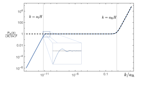
(a) Power spectra evaluated at reheating $a=a_{\rm R}$, where $a_{\rm I}=10^{-12}a_{\rm R}$ in units where $H$ is set to $2\pi$.

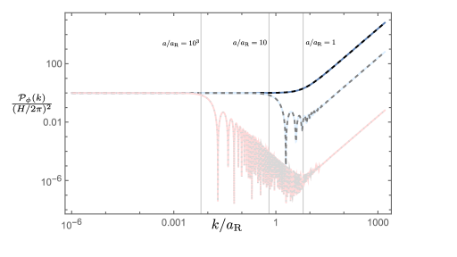
(b) Power spectra evaluated at different times during radiation domination.

Figure 1: Power spectrum comparison for a massless test scalar field with past infinite vs finite duration dS inflation (dashed and bold lines, respectively) matched to a terminal stage of radiation domination. Finite duration inflation cures the would be IR divergences, leaving only UV divergences to attend to.

The UV divergence is unsurprisingly unchanged, and can be subtracted with a cosmological constant counterterm were one to impose a cutoff in physical momenta.

In computing the energy density $\rho$, we begin with

$$\lim_{y\to x}\rho(\tau;x,y)=\frac{1}{4\pi^{2}a^{2}}\int_{0}^{\infty}k^{2}\,dk\left[k^{2}\mathcal{|}\phi^{\rm RD}_{k}(\tau)|^{2}+|\phi^{\rm RD\prime}_{k}(\tau)|^{2}\right]$$ (63)

and use Eq. 54 to express the energy density during radiation domination as

$$\rho = \frac{1}{8\pi^{2}a^{4}}\int_{0}^{\infty}\,\frac{dk}{k}\left[k^{4}\left(2+\frac{a_{\rm R}^{4}H^{2}}{a^{2}k^{2}}\right)\left(1+2|\beta^{\rm R}_{k}|^{2}_{\rm power}\right)+\{{\rm osc}\}\right],$$

$$:= \int_{0}^{\infty}\,\frac{dk}{k}\left[\Omega^{\phi}_{\rm power}(k)+\Omega^{\phi}_{\rm osc}(k)\right]$$

where the integrated contribution of $\Omega^{\phi}_{\rm osc}$, defined as $\rho_{\rm osc}$ is given in Eq. B, where it is explicitly shown not to contribute to any UV divergences. As was the case with the two point function, the contributions form Eq. 60 that nominally appear to aggravate IR divergences in the context of Eq. III.2 are canceled by contributions from the oscillatory terms that freeze out in the IR. One can expand the sum of all contributions in the IR to find the IR safe scaling $\Omega^{\phi}_{\rm tot}\propto k^{4}$, to be compared to what would have been obtained had there been no pre-inflationary phase, where $\Omega^{\phi}_{\rm tot}\propto k^{2}$. We illustrate this behavior, and the processing of the logarithmic spectra power density as we go deeper into the radiation dominated regime in Fig. 2, where the sub-horizon decay compensates for the $k^{2}$ scaling for the modes that exited the Hubble horizon during inflation to produce a scale invariant spectral density during radiation domination. We further note the additional long wavelength suppression of the spectral density for a pre-inflationary phase relative to past eternal dS.

(a)

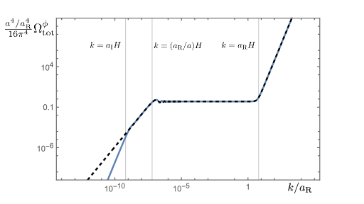
(b)

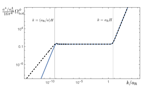
(c)

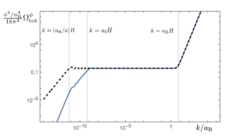
(d)

Figure 2: Power spectral energy density for a massless test scalar field comparing past infinite vs finite duration de Sitter inflation (dashed and bold lines, respectively) matched to a terminal stage of radiation domination. The panels are evaluated at subsequent times during radiation domination, with $a_{\rm I}=10^{-10}a_{\rm R}$, and with $a/a_{\rm R}=1,10^{-8},10^{-10},$ and $10^{-12}$, respectively, in units where $H=2\pi$.

Returning to Eq. III.2, we see that upon inserting Eq. 60, the only divergences that need to be regulated are given by the contributions

$$\rho_{\rm div}=\frac{1}{8\pi^{4}a^{4}}\int_{-\infty}^{\infty}d^{4}k\left(1+\frac{H^{4}a_{\rm R}^{4}+H^{4}a_{\rm I}^{4}}{2k^{4}}\right)+\frac{1}{8\pi^{4}a^{6}}\int_{-\infty}^{\infty}d^{4}k\frac{a_{\rm R}^{4}H^{2}}{2k^{2}},$$ (65)

where again we recast the logarithmic integration into the formally equivalent 4D Euclidean form as per Eq. 16, and change integration variables to physical momenta $q=k/(a_{\rm R}H)$. We stress that all factors of $H$ in the expressions above correspond to the Hubble parameter during the intermediate phase on inflation, which is presumed dS and therefore fixed as per Eq. 53.

One can proceed from here as we did in the previous subsection in comparing the results from imposing cutoffs in physical momenta with that of dimensionally regularizing factorized scaleless integrals for the energy density, with the caveat that the counterterms are strictly speaking only to be identified only through a scheme that preserves diffeomorphism invariance as per the discussion at the end of the previous subsection. By imposing cutoffs in physical momenta: $k=a\Lambda_{\rm UV}$, we see that the first term in Eq. 65 corresponds to a divergence of the form

$$\frac{1}{8\pi^{4}a^{4}}\int_{-\infty}^{\infty}\,d^{4}k=\frac{1}{4\pi^{2}a^{4}}\int_{0}^{a\Lambda_{\rm UV}}\,k^{3}dk=\frac{\Lambda_{\rm UV}^{4}}{16\pi^{2}},$$ (66)

and the third term corresponds to a divergence of the form

$$\frac{1}{8\pi^{4}a^{6}}\int_{-\infty}^{\infty}\,d^{4}k\frac{a_{\rm R}^{4}H^{2}}{2k^{2}}=\frac{a_{\rm R}^{4}H^{2}}{8\pi^{2}a^{6}}\int_{0}^{a\Lambda_{\rm UV}}\,kdk=\frac{\Lambda_{\rm UV}^{2}}{16\pi^{2}}\frac{H^{2}}{(a/a_{\rm R})^{4}},$$ (67)

which would nominally be subtracted by a counterterm proportional to $R$ were we to insist on hard cutoff cutoff regularization. The former, when varied with respect to the metric yields the contribution $R_{\mu\nu}\sim 1/a^{4}$ and thus corresponds to a renormalization of Newton’s constant. Finally, the second term in Eq. 65 result in a divergence of the form

$$\frac{1}{8\pi^{4}a^{4}}\int_{-\infty}^{\infty}\,d^{4}k\>\left(\frac{a_{\rm R}^{4}H^{4}+a_{\rm I}^{4}H^{4}}{2k^{4}}\right)=\frac{1}{8\pi^{2}a^{4}}\int_{a\Lambda_{\rm IR}}^{a\Lambda_{\rm UV}}\,\frac{dk}{k}\left(a_{\rm R}^{4}H^{4}+a_{\rm I}^{4}H^{4}\right)=\frac{H^{4}(1+e^{-4\mathcal{N}_{\rm tot}})}{8\pi^{2}(a/a_{\rm R})^{4}}\log\frac{\Lambda_{\rm UV}}{\Lambda_{\rm IR}},$$ (68)

where the scale $\Lambda_{\rm IR}$ does not have the same significance as before given the IR safe behavior of the spectral density, and where the above also corresponds to a renormalization of Newton’s constant. We note that the scales corresponding to the beginning and end of inflation appear in the coefficient of the logarithm, whereas the UV scale corresponding to the unknown completion the theory appears inside the logarithm.

Were we to now dimensionally regularize the divergences as advised, we can perform a similar factorization of the scaleless integrals as in the previous subsection. The nominally power law divergent parts can be isolated as

$$\rho^{\rm UV}_{\rm div} = \frac{1}{8\pi^{4}a^{4}}\int_{-\infty}^{\infty}\,d^{4}k\left(1+\frac{a_{\rm R}^{4}H^{2}}{2a^{2}k^{2}}\right)$$

$$= \frac{1}{8\pi^{4}a^{4}}\int_{-\infty}^{\infty}\,d^{4}k\left[\frac{k^{2}}{(k^{2}+m^{2})}+\frac{m^{2}}{(k^{2}+m^{2})}+\frac{a_{\rm R}^{4}H^{2}}{2a^{2}}\left(\frac{1}{(k^{2}+m^{2})}+\frac{m^{2}}{k^{2}(k^{2}+m^{2})}\right)\right],$$

where we see that power law UV divergences cancel among themselves, and so do not necessitate any counterterms. On the other hand, the UV divergent logarithmic term can be isolated and factorized as

$$\rho^{\rm log}_{\rm div} = \frac{1}{8\pi^{4}a^{4}}\int_{-\infty}^{\infty}\,d^{4}k\>\left(\frac{a_{\rm R}^{4}H^{4}+a_{\rm I}^{4}H^{4}}{2k^{4}}\right)$$

$$= \frac{1}{8\pi^{4}a^{4}}\int_{-\infty}^{\infty}\,d^{4}k\left(\frac{a_{\rm R}^{4}H^{4}+a_{\rm I}^{4}H^{4}}{2}\right)\left(\frac{1}{k^{2}(k^{2}+m^{2})}+\frac{m^{2}}{k^{4}(k^{2}+m^{2})}\right)$$

By isolating the logarithmic UV poles, we find

$$\rho^{\rm log}_{\rm div}=\frac{H^{4}(1+e^{-4\mathcal{N}_{\rm tot}})}{8\pi^{2}(a/a_{\rm R})^{4}}\left[\frac{1}{\delta_{\rm UV}}+1-\gamma_{E}+\log\left(\frac{\mu}{H}\right)\right]$$ (71)

from which we read off an identical coefficient as computed in Eq. 68. For completeness, we show in Appendix C that the coefficient of the logarithmic divergence obtained from point split regularization in the FRLW slicing is also identical, with the same power law divergences identified in physical cutoff regularization up to the expected scheme dependence in the coefficients of the latter.

To summarize our findings in this subsection: the scales corresponding to the beginning and end of inflation must in principle be separated from any UV and IR scales parameterizing the unknown completion of our theory and well defined observable quantities. Although physical quantities cannot depend on the latter, they may certainly depend on the former. We found that all IR divergences encountered in the simplified settings we worked in were regulated by the existence of a pre-inflationary phase, and therefore an artifact of the approximation of a past infinite dS phase. A highly pertinent question is whether this persists once we move to incorporate higher point interactions and couplings with other test fields. Unsurprisingly, UV divergences persist for backgrounds corresponding to finite duration inflation, and the scale corresponding to the end of inflation parameterizes their coefficients rather than regulating them. Upon subtraction of these divergences with local counterterms and the imposition of renormalization conditions, one is able to draw meaningful physical conclusions. However, the two point function and stress tensor of a test scalar field are of relatively academic interest given the assumed negligibility of the scalar field background, and therefore inability to fix renormalization conditions from observation. The analogous set of questions for vacuum tensor perturbations presents a far more interesting application given the assumption of an evolving background gravitational field (that of FRLW cosmology), perturbations around which represent gravitational waves, which is where we turn our attention towards next.

IV Gravitational waves

Before delving into the substance of this section, it is informative to contrast the results obtained in the previous section to analogous expressions typically found in the literature in the context of gravitational waves (see e.g. [71, 72, 73, 74, 75, 76, 77, 78, 79, 80, 81, 82, 83, 84]), where imposing hard cutoffs on the energy density of gravitational waves results in expressions of the form:

$$\rho_{\mathrm{GW}}\simeq\frac{A_{t}}{32\pi G_{N}}\left(\frac{k_{\mathrm{UV}}}{k_{*}}\right)^{n_{t}}\frac{1}{2n_{t}}\frac{1}{a^{4}}\propto\frac{1}{a^{4}}\left[\frac{1}{n_{t}}+\log\frac{k_{\rm UV}}{k_{*}}\right],$$ (72)

where $k_{*}$ is some reference IR scale, and the approximation is only valid when $n_{t}\to 0$ [71]. We deconstruct and rederive the energy density for vacuum tensor perturbations in what follows, but before doing so, it is useful to compare what one would have obtained in retracing the steps leading to Eq. 72 for a massless test scalar field, which would have resulted in the expression

$$\rho\simeq\lim_{n_{s}\to 1}\frac{A_{s}}{32\pi G_{N}}\left(\frac{k_{\mathrm{UV}}}{k_{*}}\right)^{n_{\rm s}-1}\frac{1}{2(n_{s}-1)}\frac{1}{a^{4}}\propto\frac{1}{a^{4}}\left[\frac{1}{n_{s}-1}+\log\frac{k_{\rm UV}}{k_{*}}\right],$$ (73)

which can directly be compared to the divergences computed in Eqs. 66 - 68 from hard cutoffs in physical momenta and Eq. 71 from dimensional regularization, all of which are understood to be intermediate expressions that are to be subtracted and renormalized.

An immediate reservation one might express for expressions such as Eq. 72 is the appearance of cutoffs in what should be a physical result. Although one might argue that the effects of UV and IR modes are negligible relative to what can be extracted from Eq. 72, its form nevertheless suggests that the expression above is an intermediate result on the way to computing a physical energy density. Moreover, one might be concerned in applying the formula Eq. 72 to the case of blue tilted spectra (i.e. for positive $n_{t}\sim\mathcal{O}(1)$, so that $\rho_{\rm GW}\sim(k_{\rm UV}/k_{*})^{n_{t}}$ as derived in e.g. [71]), that some part of this expression is nothing other than the Fourier transform of a UV divergence that gets subtracted in the usual way. The particular case of $n_{t}=3$ is particularly interesting in this context, as part of it is exactly mimicked by the familiar quadratic UV divergence from the perspective of cutoff regularization, necessitating greater care in the interpretation of such power spectra. In spite of this caution, it is both practical and straightforward to follow through this process to the end to ensure that one is computing well defined physical observables. In the specific context of vacuum tensor perturbations, however, additional subtleties must be accounted for.

The formula for the stress energy tensor of gravitational waves was first derived by Isaacson in the context astrophysically sourced gravitational waves [85] (see also [86, 87]), which is nevertheless extensively referenced in computations of the stress energy tensor of cosmological gravitational wave backgrounds, and is given by

$$\rho^{\rm Isc}_{\rm gw}=\frac{1}{32\pi a^{2}G_{N}}\left\langle h^{\prime}_{ij}(\tau,k)h^{\prime ij}(\tau,k)\right\rangle.$$ (74)

However, retracing the steps used in its derivation, it becomes immediately clear that one needs to proceed with extra care for applications in a cosmological context, in particular when considering questions of renormalized stress tensors in prescriptions that involve integrations over all momenta. This is because the Isaacson form presumes a prior scale separation between fast and slow frequencies defined relative to the curvature scale of the background (a criteria that is time dependent), and repeatedly relies on this scale separation along with the implicit averaging prescription to facilitate various approximations resulting in the simplified final form Eq. 74. In the context of an expanding spacetime, with modes of observational relevance that might have crossed any a priori defined scale more than once over cosmic evolution, undoing the steps that relied on these approximations is warranted. We do so in Appendix D, retracing the derivation of the stress tensor for gravitational waves, finding the resulting expression for the energy density:

$$\rho^{\rm Imp}_{\rm gw}=\frac{1}{8\pi G_{N}}\left\langle\frac{1}{8a^{2}}h_{ij}^{\prime}h^{\prime ij}-\frac{3}{8a^{2}}\partial_{k}h_{ij}\partial^{k}h^{ij}-\frac{1}{2a^{2}}h_{ij}\partial_{k}\partial^{k}h^{ij}+\frac{1}{4a^{2}}\partial_{k}h_{ij}\partial^{j}h^{ik}+\frac{\mathcal{H}}{a^{2}}h_{j}{}^{i}h^{\prime}_{i}{}^{j}\right\rangle\>,$$ (75)

where $\mathcal{H}:=a^{\prime}/a$. The derivation is straightforward, and follows from the same starting point as the derivation leading to Eq. 74, but with any steps that invoked a time averaging prescription or frequency separation left undone (we elaborate on the details in Appendix D).

It is worth stressing that Eq. 75 is the temporal component of a covariantly conserved tensor, and is under no obligation to conserved in isolation. This is a corollary of the fact that on FRLW backgrounds, a locally conserved energy cannot be defined. Moreover, it is also under no obligation to be positive definite. In fact, were one to insist of constructing the spectral density associated with the vacuum expectation value of Eq. 75, one can show that it crosses zero at a comoving scale corresponding to the horizon scale at any given time, consistent with the operational ambiguity of associating a background/fluctuation split for wavelengths commensurate with the background curvature. However, none of this is of any operational concern for our purposes, as we stress that Eq. 75 is to be viewed as the components of a covariantly conserved tensor corresponding to a massless spin two excitation, whose role in renormalization of background quantities is well understood in the covariant context, but obscured and widely conflated for a physical contribution to the number of relativistic species in foliation specific computations as we elaborate upon next. The specific computation we are interested in performing is the renormalization of the graviton stress tensor on a background corresponding to radiation domination preceded by a finite period of inflation. In doing so, we will compare and contrast the results obtained from both the Isaacson and improved forms of the stress tensor, before revisiting the question of $N_{\rm eff}$ bounds from vacuum tensor modes and concluding.

IV.1 Divergences – vacuum tensor modes and finite duration inflation

Working in transverse-traceless (TT) gauge (see Appendix D for the relevant details and caveats), we expand the tensor perturbations as

$$\hat{h}_{ij}(\tau,x)=\sum_{r=+,x}\int\frac{d^{3}k}{M_{\rm pl}\left(2\pi\right)^{3}}e^{ix\cdot k}\left[\epsilon_{ij}^{r}(k)\hat{a}_{k}\gamma_{k}(\tau)+\epsilon_{ij}^{r*}(-k)\hat{a}_{-k}^{{\dagger}}\gamma^{*}_{k}(\tau)\right]$$ (76)

with polarization tensors normalized as $\epsilon_{ij}^{s}\epsilon_{ij}^{r*}=4\delta^{rs}$, $k^{i}\epsilon_{ij}^{r}=0$. The normalizations are chosen so that the relevant mode functions during inflation and the pre and post-inflationary phases of radiation domination are given for each polarization just as for massless minimally coupled scalars. These are:

$$\gamma^{\rm PI}_{k}(\tau) = \frac{1}{a}\frac{1}{\sqrt{2k}}e^{-ik\tau_{\rm I}\left(2-\frac{a}{a_{\rm R}}e^{\mathcal{N}}_{\rm tot}\right)}$$ (77)

$$\gamma^{\prime\rm PI}_{k}(\tau) = -\frac{1}{a^{2}\sqrt{2k}}\frac{a_{\rm I}}{\tau_{\rm I}}e^{-ik\tau_{\rm I}\left(2-\frac{a}{a_{\rm R}}e^{\mathcal{N}}_{\rm tot}\right)}\left(-1+ik\tau_{\rm I}\frac{a}{a_{\rm I}}\right),$$

during the pre-inflationary phase,

$$\gamma_{k}^{\rm I}(\tau) = \frac{H}{\sqrt{2k^{3}}}\left[\alpha_{k}^{\rm I}e^{i\frac{k}{aH}}\left(1-\frac{ik}{aH}\right)+\beta_{k}^{\rm I}e^{-i\frac{k}{aH}}\left(1+\frac{ik}{aH}\right)\right]$$ (78)

$$\gamma^{\prime\rm I}_{k}(\tau) = -\frac{H}{\sqrt{2k^{3}}}\left[\alpha_{k}^{\rm I}e^{i\frac{k}{aH}}\frac{k^{2}}{aH}+\beta_{k}^{\rm I}e^{-i\frac{k}{aH}}\frac{k^{2}}{aH}\right],$$

during inflation, and

$$\gamma^{\rm RD}_{k}(\tau) = \frac{1}{a}\frac{1}{\sqrt{2k}}\left[\alpha_{k}^{\rm R}e^{-ik\tau_{\rm R}\left(2-\frac{a}{a_{\rm R}}\right)}+\beta_{k}^{\rm R}e^{ik\tau_{\rm R}\left(2-\frac{a}{a_{\rm R}}\right)}\right]$$ (79)

$$\gamma^{\prime\rm RD}_{k}(\tau) = \frac{a_{\rm R}}{a^{2}\tau_{\rm R}}\frac{1}{\sqrt{2k}}\left[\alpha_{k}^{\rm R}e^{-ik\tau_{\rm R}\left(2-\frac{a}{a_{\rm R}}\right)}\left(1-ik\tau_{R}\frac{a}{a_{\rm R}}\right)+\beta_{k}^{\rm R}e^{ik\tau_{\rm R}\left(2-\frac{a}{a_{\rm R}}\right)}\left(1+ik\tau_{\rm R}\frac{a}{a_{\rm R}}\right)\right]$$

during the terminal radiation dominated phase. The corresponding Bogoliubov coefficients are the same as those given in Eq. 57 and Eq. III.2.

An immediate corollary of the above is that the two point correlation function of each graviton polarization is identical to that of a massless, minimally coupled scalar. Therefore, as illustrated in Figs. 1(a) and 1(b), one finds that the IR divergences exhibited on a past infinite dS background are also cured for the graviton two point function on a background corresponding to finite duration inflation.

The energy density of gravitational waves presuming the Isaacson form of the stress tensor Eq. 74 results in (with the reduced Planck mass defined as $M^{2}_{\rm pl}=\frac{1}{8\pi G_{N}}$):

$$\rho_{\rm gw}^{\rm Isc} = \lim_{y\to x}\rho_{\rm gw}(\tau;x,y)=\frac{1}{\pi^{2}a^{2}}\int_{0}^{\infty}dk\ k^{2}\>\left[\gamma^{{}^{\prime}\rm RD}_{k}\gamma^{{}^{\prime}\rm RD*}_{k}\right]$$ (80)

as the tensor mode counterpart of Eq. 63, after having summed the contributions from the two independent polarizations.

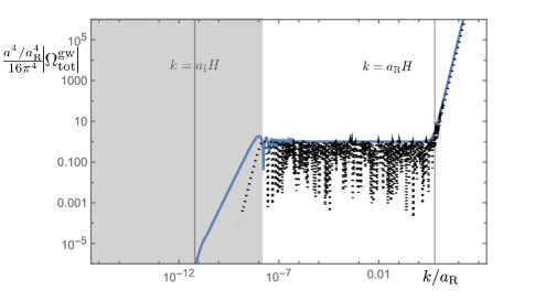
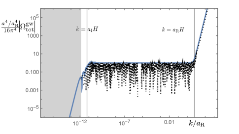
Figure 3: Power spectral density of the Isaacson stress tensor (dashed lines) evaluated at $a=10^{9}a_{\rm R}$ (left) and $a=10^{13}a_{\rm R}$ (right), with $a_{\rm I}=10^{-12}a_{\rm R}$ in units where $H$ is set to $2\pi$. The blue line is the comparison to the spectral density of the improved stress tensor. The gray shaded regions correspond to super-horizon scales, which are outside the domain of validity of the Isaacson stress tensor (where we note that the oscillations would not appear in its time averaged form), and also where the spectral density for the improved stress tensor nominally becomes negative (cf. discussion below Eq. 75).

Using the mode functions specified by Eqs. 79, the relations III.2, and tracing through the steps of the previous section, we find

$$\rho_{\rm gw}^{\rm Isc} = \frac{1}{2\pi^{2}a^{4}}\int_{0}^{\infty}\frac{dk}{k}\>k^{4}\left[\left(1+\frac{a_{\rm R}^{4}H^{2}}{a^{2}k^{2}}\right)\left(1+2|\beta^{\rm R}_{k}|^{2}_{\rm power}\right)+\{{\rm osc}\}\right],$$

$$:= \int_{0}^{\infty}\,\frac{dk}{k}\left[\Omega^{\rm gw}_{\rm power}(k,\tau)+\Omega^{\rm gw}_{\rm osc}(k,\tau)\right],$$

where, as we did for the scalar case, we similarly separate the spectral density into oscillatory and power law contributions, and all contributions to $\rho_{\rm gw}$ can be found in Eq. B. Even though the Isaacson form of the stress tensor is not strictly valid when incorporating wavelengths greater than the Hubble scale at any given time, naïvely persisting with it for all wavelengths would show an IR regular spectral density $\Omega^{\rm gw}_{\rm total}\propto k^{2}$, with oscillatory contributions contributions giving negligible contributions in the UV. Consequently, one only has the resulting UV divergent contributions to regulate:

$$\rho^{\rm Isc}_{\rm gw,div} = \frac{1}{4\pi^{4}a^{4}}\int_{-\infty}^{\infty}\,d^{4}k\>\left(1+\frac{a_{\rm R}^{4}H^{4}+a_{\rm I}^{4}H^{4}}{2k^{4}}+\frac{a_{\rm R}^{4}H^{2}}{a^{2}k^{2}}\right),$$ (82)

which up to overall factors, is formally identical to the contributions Eq. 65, and whose subtraction proceeds along the same lines.

Were we to consider the improved stress tensor Eq. 75 (which does not invoke a scale separation or time averaging prescription), one would obtain

$$\rho_{\rm gw}^{\rm Imp} = \frac{1}{2\pi^{2}a^{2}}\int_{0}^{\infty}dk\ k^{2}\>\left[\gamma^{{}^{\prime}\rm RD}_{k}\gamma^{{}^{\prime}\rm RD*}_{k}+k^{2}\gamma^{\rm RD}_{k}\gamma^{\rm RD*}_{k}+4\mathcal{H}\left(\gamma^{{}^{\prime}\rm RD}_{k}\gamma^{\rm RD*}_{k}+\gamma^{\rm RD}_{k}\gamma^{{}^{\prime}\rm RD*}_{k}\right)\right]$$ (83)

as the counterpart of Eq. 80 that is now valid for for all wavelengths. Using the mode functions and normalizations specified above, one finds

$$\rho_{\rm gw}^{\rm Imp} = \frac{1}{2\pi^{2}a^{4}}\int_{0}^{\infty}\frac{dk}{k}\>k^{4}\left[\left(1-\frac{7a_{\rm R}^{4}H^{2}}{2a^{2}k^{2}}\right)\left(1+2|\beta^{\rm R}_{k}|^{2}_{\rm power}\right)+\{{\rm osc}\}\right],$$

$$:= \int_{0}^{\infty}\,\frac{dk}{k}\left[\Omega^{\rm gw}_{\rm power}(k,\tau)+\Omega^{\rm gw}_{\rm osc}(k,\tau)\right]$$

where we can again separate the spectral density into oscillatory and power law contributions, where all contributions to $\rho^{\rm Imp}_{\rm gw}$ can be found in Eq. B.

One again finds that the spectral density summing all contributions in the IR goes as $\Omega^{\rm gw}_{\rm total}\propto k^{2}$, albeit with a negative overall coefficient (cf. the discussion below Eq. 75), with the following divergent contributions in the UV that necessitate subtraction

$$\rho_{\rm gw,div}^{\rm Imp} = \frac{1}{4\pi^{4}a^{4}}\int_{-\infty}^{\infty}\,d^{4}k\>\left(1+\frac{a_{\rm R}^{4}H^{4}+a_{\rm I}^{4}H^{4}}{2k^{4}}-\frac{7\,a_{\rm R}^{4}H^{2}}{2a^{2}k^{2}}\right).$$ (85)

For illustrative purposes, we plot the power spectral densities of the (time unaveraged) Isaacson and improved forms of the stress tensors in Fig. 3. For sub-horizon modes, where a positive spectral density results, the improved stress tensor evaluated at any given time does not exhibit oscillations. In proceeding to regularizing divergences, we can identity the various UV divergences is different schemes, finding identical coefficients for the log divergences in all of them. By imposing cutoffs in physical momenta ($k=a\Lambda_{\rm UV}$) on the identifiably UV-divergent terms above, we obtain

$$\frac{1}{2\pi^{2}a^{4}}\int_{0}^{a\Lambda_{\rm UV}}dk\>k^{3}-\frac{7}{2}\frac{a_{\rm R}^{4}H^{2}}{2\pi^{2}a^{6}}\int_{0}^{a\Lambda_{\rm UV}}dk\>k=\frac{\Lambda_{\rm UV}^{4}}{8\pi^{2}}-\frac{7H^{2}\Lambda_{\rm UV}^{2}}{8\pi^{2}(a/a_{\rm R})^{4}}$$ (86)

and

$$\frac{1}{4\pi^{2}a^{4}}\int_{a\Lambda_{\rm IR}}^{a\Lambda_{\rm UV}}\,\frac{dk}{k}\left(a_{\rm R}^{4}H^{4}+a_{\rm I}^{4}H^{4}\right)=\frac{H^{4}\left(1+e^{-4\mathcal{N}_{\rm tot}}\right)}{4\pi^{2}(a/a_{R})^{4}}\log\frac{\Lambda_{\rm UV}}{\Lambda_{\rm IR}}.$$ (87)

If instead we were to now isolate the power law UV divergent parts and dimensionally regularize, we would obtain

$$\rho^{\rm Imp}_{\rm gw,div} \supset \frac{1}{4\pi^{4}a^{4}}\int_{-\infty}^{\infty}\,d^{4}k-\frac{7a_{\rm R}^{2}}{4\pi^{4}a^{6}}\int_{-\infty}^{\infty}\,d^{4}k\>\left(\frac{a_{\rm R}^{2}H^{2}}{2k^{2}}\right)$$

$$= \frac{1}{4\pi^{4}a^{4}}\int_{-\infty}^{\infty}\,d^{4}k\left[\frac{k^{2}}{(k^{2}+m^{2})}+\frac{m^{2}}{(k^{2}+m^{2})}-\frac{7}{2}\frac{a_{\rm R}^{4}H^{2}}{2a^{2}}\left(\frac{1}{(k^{2}+m^{2})}+\frac{m^{2}}{k^{2}(k^{2}+m^{2})}\right)\right]$$

which, as for the dimensionally regularized scalar case Eq. III.2, has the divergent contributions canceling among themselves and not necessitating any counterterms. The logarithmic divergence can be expressed as

$$\rho^{\rm Imp}_{\rm gw,div} \supset \frac{1}{4\pi^{4}a^{4}}\int_{-\infty}^{\infty}\,d^{4}k\>\left(\frac{a_{\rm R}^{4}H^{4}+a_{\rm I}^{4}H^{4}}{2k^{4}}\right)=\frac{H^{4}\left(1+e^{-4\mathcal{N}_{\rm tot}}\right)}{4\pi^{2}(a/a_{\rm R})^{4}}\left[\frac{1}{\delta_{\rm UV}}+1-\gamma_{E}+\log\left(\frac{\mu}{H}\right)\right].$$ (89)

Lastly, one can point split regularize Eq. 82 by commuting the coincident limit with the momentum integrations, so that one has to evaluate

$$\rho_{\rm gw}^{\rm Imp} = \frac{1}{4\pi^{2}a^{4}r}\int_{0}^{\infty}\,k^{2}dk\,\sin kr\>\left[\left(1-\frac{7a_{\rm R}^{4}H^{2}}{2a^{2}k^{2}}\right)\left(1+2|\beta^{\rm R}_{k}|^{2}_{\rm power}\right)+\{{\rm osc}\}\right],$$ (90)

which can be shown to result in the UV divergent contributions

$$\rho^{\rm Imp}_{\rm gw,div}=\lim_{\sigma\to 0}\left\{-\frac{1}{\pi^{2}\sigma^{4}}-\frac{7H^{2}}{4\pi^{2}\sigma^{2}(a/a_{\rm R}^{4})}+\frac{H^{4}\left(1+e^{-4\mathcal{N}_{\rm tot}}\right)}{4\pi^{2}(a/a_{\rm R})^{4}}\left[1-\gamma_{E}-\log{k_{p}\sigma}\right]\right\},\leavevmode\nobreak\ \leavevmode\nobreak\ \leavevmode\nobreak\ \leavevmode\nobreak\ {\rm(point-split)}$$ (91)

where as before $\sigma=ar$ and $k_{p}:=k/a$ are physical quantities. We mote that the coefficient of the logarithmic divergence is identical, with the minus sign reflecting the fact that $\sigma\to 0$ inside the point split logarithm, whereas $\Lambda_{\rm UV}\to\infty$ with hard cutoff regularization, the results of which can be collected and summarized as

$$\rho^{\rm Imp}_{\rm gw,div} = \lim_{\Lambda_{\rm UV}\to\infty}\left\{\frac{1}{2\pi^{2}}\frac{\Lambda_{\rm UV}^{4}}{4}-\frac{7}{2}\frac{a_{\rm R}^{4}H^{2}}{2\pi^{2}a^{4}}\frac{\Lambda_{\rm UV}^{2}}{2}+\frac{H^{4}\left(1+e^{-4\mathcal{N}_{\rm tot}}\right)}{4\pi^{2}(a/a_{\rm R})^{4}}\log\frac{\Lambda_{\rm UV}}{\Lambda_{\rm IR}}\right\},\leavevmode\nobreak\ \leavevmode\nobreak\ \leavevmode\nobreak\ \leavevmode\nobreak\ {\rm(cutoff)}$$ (92)

and also compared to the answer obtained via dimensional regularization

$$\rho^{\rm Imp}_{\rm gw,div} = \lim_{\delta_{\rm UV}\to 0}\left\{\frac{H^{4}\left(1+e^{-4\mathcal{N}_{\rm tot}}\right)}{4\pi^{2}(a/a_{R})^{4}}\left[\frac{1}{\delta_{\rm UV}}+1-\gamma_{E}+\log\left(\frac{\mu}{H}\right)\right]\right\}.\leavevmode\nobreak\ \leavevmode\nobreak\ \leavevmode\nobreak\ \leavevmode\nobreak\ \leavevmode\nobreak\ \leavevmode\nobreak\ \leavevmode\nobreak\ \leavevmode\nobreak\ \leavevmode\nobreak\ \leavevmode\nobreak\ \leavevmode\nobreak\ \leavevmode\nobreak\ \leavevmode\nobreak\ \leavevmode\nobreak\ {\rm(dim-reg)}$$ (93)

After having subtracting divergences with the appropriate counterterms, a finite remainder remains that needs to be fixed by the imposition of renormalization conditions by observations at a given scale. This in order to have a predictive theory with which we can calculate the results for any subsequent observations. As cautioned in the previous section, one may not be able to do this reliably unless one uses regularization schemes that preserve the symmetries of the background so that the required counterterms can be consistently identified (see Appendix A for more details). For this reason, we stick to dimensional regularization in what follows, although covariant point splitting methods also offer a practical alternative [3, 91, 92, 93, 94, 95, 96].

In order to understand which counterterms we need to add in order to reabsorb the divergences in dimensional regularization, we need only to look at the scale factor dependence of the divergences in Eq. 119. However, we immediately notice that the divergences we have computed do not necessitate higher derivative counterterms beyond those already in the Einstein Hilbert action. In order to understand why this is, we trace through a treatment that uses adiabatic regularization to renormalize the stress tensor of a non-minimally coupled test scalar field [97], where mode functions are adiabatically expanded in order to regularize divergences and identify counterterms. Higher orders in the adiabatic expansion necessitate successively higher order counterterms. The adiabatic solution of order zero is regularized by a cosmological constant counterterm, the second order solution by a curvature counterterm, with curvature squared counterterms needed to renormalize divergences that appear only at fourth order in the adiabatic expansion. In our case the adiabatic solution of order four is null and non-vanishing curvature squared counterterms would only be necessitated were one to consider couplings to other matter fields, or by incorporating the effects of loops and higher order gravitational and matter coupling non-linearities.

V Renormalized stress tensors (and $N_{\rm eff}$ bounds)

We turn our attention in this section to the second and most consequential step in the process of renormalization – that of extracting physical observables after imposing renormalization conditions. We begin the discussion with the relatively academic exercise of renormalizing the stress tensor of a test scalar field on a background that transitions in and out of inflation. By virtue of not having a classically evolving background and energy density, the only effects of a test scalar will be in renormalizing background couplings in the context of the effective theory of gravity [67, 68, 69, 70]. We return to the more interesting and physically relevant case of primordial gravitational waves next.

Our starting point is the bare matter and gravitational actions, along with the requisite counterterms:

$$S=S_{\rm EH}+S_{\rm bg}+S_{\phi}+S_{\rm ct}.$$ (94)

In order to impose renormalization conditions after having regularized divergences, we first consider the background equations of motion

$$\frac{1}{8\pi G_{B}}\left(R_{\mu\nu}-\frac{1}{2}Rg_{\mu\nu}\right)=T^{\rm bg}_{\mu\nu}+T^{\phi}_{\mu\nu}+T^{\rm ct}_{\mu\nu},$$ (95)

where we stress that the couplings that appear in Eq. 94 are to be understood as bare couplings, and the presence of the counterterm shifts the tadpole condition in a manner that we will shortly make precise. Given the consistency of dimensional regularization with general covariance, we can proceed by considering the above for any given component. For the 00 component, we have

$$-\frac{R_{0}{}^{0}}{8\pi G_{B}}=\rho^{\rm cl}_{\rm bg}+\rho_{\phi}+\rho_{\rm ct},$$ (96)

where $\rho^{\rm cl}_{\rm bg}$ is the to be renormalized classical background energy density that sources the expanding geometry around which we have computed the stress tensor for the test scalar field, with corresponding energy density $\rho_{\phi}$ defined as

$$\rho_{\phi}:=\rho^{\rm cl}_{\phi}-\langle T^{0}{}_{0}\rangle\equiv-\langle T^{0}{}_{0}\rangle,$$ (97)

where $\rho_{\phi}^{\rm cl}\equiv 0$ for a test scalar by assumption. The background satisfies

$$-R_{0}{}^{0}=-\frac{3}{a^{2}}\left(\frac{a^{\prime}}{a}\right)^{\prime}=\frac{3H^{2}}{(a/a_{\rm R})^{4}}$$ (98)

via Eq. III.2 during the terminal radiation dominated phase, where it is to be stressed again that $H$ is the Hubble constant during the intermediate phase of inflation that enters the definition of the scale factor during radiation domination via Eq. III.2. We need to identify the counterterm that absorbs the divergence exhibited in Eq. 71:

$$\frac{1}{8\pi G_{B}}\frac{3H^{2}}{(a/a_{R})^{4}}=\rho^{\rm cl}_{\rm bg}+\frac{H^{4}(1+e^{-4\mathcal{N}_{\rm tot}})}{8\pi^{2}(a/a_{\rm R})^{4}}\left[\frac{1}{\delta_{\rm UV}}+1-\gamma_{E}+\log\left(\frac{\mu}{H}\right)\right]+\rho_{\rm ct}+\rho_{\phi,\rm finite},$$ (99)

where $\rho_{\rm finite}\equiv\rho_{\phi}-\rho_{\rm\phi,div}$. We are immediately presented with a choice here – after subtracting the pole, do we proceed to (multiplicatively) renormalize Newton’s constant, or (additively) renormalize the background whose unshifted value is determined by $\rho^{\rm cl}_{\rm bg}$? It turns out that this choice is rendered moot by the tadpole condition that determines the background equations of motion at any given order in $\hbar$, in that whichever choice we make will lead us to the same shifted tadpole condition. We thus proceed by reabsorbing the pole by adding a counterterm that multiplies the Ricci scalar in the Einstein Hilbert action with coefficient $B$ defined as

$$\rho_{\rm ct}=\frac{3H^{2}}{(a/a_{R})^{4}}\left(\frac{B_{-1}}{\delta_{\rm UV}}+B_{0}\right).$$ (100)

By assigning

$$B_{-1}=-\frac{H^{2}(1+e^{-4\mathcal{N}_{\rm tot}})}{24\pi^{2}},$$ (101)

one subtracts the pole contribution. By defining a scale dependent gravitational coupling as

$$\frac{1}{8\pi G_{N}(\mu)}=\frac{1}{8\pi G_{B}}-B_{0}-\frac{H^{2}}{24\pi^{2}}(1+e^{-4\mathcal{N}_{\rm tot}})\left\{1-\gamma_{E}+\log\left(\frac{\mu}{H}\right)\right\},$$ (102)

we can rewrite Eq. 99 as

$$\frac{1}{8\pi G_{N}(\mu)}\frac{3H^{2}}{(a/a_{R})^{4}}=\rho^{\rm cl}_{\rm bg}+\rho_{\rm\phi,finite},$$ (103)

where the finite remainder from the counterterm and $\rho_{\phi,\rm div}$ are absorbed by the scale dependent gravitational coupling, allowing us to start imposing renormalization conditions to fix the finite parts. We do so by determining the Newtonian constant via a measurement at some energy scale $\mu_{*}$, with which we can eliminate all reference to $G_{B}$ and $B_{0}$ via

$$\frac{1}{8\pi G_{B}}=\frac{1}{8\pi G_{N}(\mu_{*})}+B_{0}+\frac{H^{2}}{24\pi^{2}}(1+e^{-4\mathcal{N}_{\rm tot}})\left\{1-\gamma_{E}+\log\left(\frac{\mu_{*}}{H}\right)\right\},$$ (104)

and substituting the result into Eq. 102 to obtain

$$\frac{1}{8\pi G_{N}(\mu)}=\frac{1}{8\pi G_{N}(\mu_{*})}-\frac{H^{2}}{24\pi^{2}}(1+e^{-4\mathcal{N}_{\rm tot}})\log\left(\frac{\mu}{\mu_{*}}\right).$$ (105)

Picking $\mu_{*}$ to be some scale where we have determined Newton’s constant to be $8\pi G_{N}(\mu_{*})=M_{\rm pl}^{-2}$ where $M_{\rm pl}=2.435\times 10^{18}$ GeV, we can finally express $G_{N}(\mu)$ as

$$8\pi G_{N}(\mu)=\frac{1}{M_{\rm pl}^{2}}\left[1-\frac{H^{2}(1+e^{-4\mathcal{N}_{\rm tot}})}{24\pi^{2}M_{\rm pl}^{2}}\log\left(\frac{\mu}{\mu_{*}}\right)\right]^{-1},$$ (106)

which can be used to express Eq. 103 in its fully covariant form as

$$G_{\mu\nu}=\frac{1}{M_{\rm pl}^{2}}T^{\rm bg,shift}_{\mu\nu}\left[1-\frac{H^{2}(1+e^{-4\mathcal{N}_{\rm tot}})}{24\pi^{2}M_{\rm pl}^{2}}\log\left(\frac{\mu}{\mu_{*}}\right)\right]^{-1},$$ (107)

where the shifted background stress tensor is defined as the sum of tree level and finite contributions on the left hand side of Eq. 103. Several things are to be immediately noted here – foremost is the minuscule nature of the scale dependence of the gravitational coupling should we phrase it that way. We could also simply view it as a multiplicative renormalization of the background matter content that sources the expansion history. Given that virtual effects from test scalar fields serve only to renormalize background quantities and impart scale dependence in observables associated to other propagating degrees of freedom (and that too, in a highly suppressed manner [63, 64, 65]), this is the furthest we can take this exercise. The situation for gravitational waves is more interesting.

Retracing the steps above with the dimensionally regularized result for gravitational waves on a finite duration background in Eq. 119, we end up with the renormalized background

$$G_{\mu\nu}=\frac{1}{M_{\rm pl}^{2}}T^{\rm bg,shift}_{\mu\nu}\left[1-\frac{H^{2}(1+e^{-4\mathcal{N}_{\rm tot}})}{12\pi^{2}M_{\rm pl}^{2}}\log\left(\frac{\mu}{\mu_{*}}\right)\right]^{-1},$$ (108)

which should be the starting point for determining any constraints on vacuum sourced primordial gravitational waves from $N_{\rm eff}$ bounds. The latter is in essence the question of how vacuum tensor perturbations renormalize the background expansion through $1/a^{4}$ contributions that mimic additional relativistic species. Unlike the case for virtual test scalars, however, gravitational waves have a classically evolving background upon which they represent perturbations – the background geometry itself. Therefore, we have additional means to potentially measure the contributions from vacuum tensor modes.

We first reconsider the spectral density for gravitational waves $\Omega^{\rm gw}(k,\tau)$, whose amplitude on the scale invariant plateau for sub-horizon modes is well defined, and given by

$$\Omega^{\rm gw}(k,\tau)=\frac{H^{4}}{16\pi^{4}(a/a_{\rm R})^{4}}\leavevmode\nobreak\ \leavevmode\nobreak\ \leavevmode\nobreak\ \leavevmode\nobreak\ \leavevmode\nobreak\ {\rm(sub-horizon)}$$ (109)

as plotted in Fig. 3. Let us presume that we have the means to determine the ratio $H^{2}/M_{\rm pl}^{2}$ during inflation via measurement of the tensor to scalar ratio at some pivot scale via B-mode anisotropy observations, or via the measurement of the spectral density of the stochastic gravitational wave background at some fixed scale via interferometeric means, or both. In the context of Eq. 108, which can now be re-expressed as

$$\frac{3H^{2}}{(a/a_{R})^{4}} = \frac{1}{M_{\rm pl}^{2}}\left(\rho_{\rm bg}^{\rm cl}+\rho_{\rm gw,finite}\right)\left[1-\frac{H^{2}(1+e^{-4\mathcal{N}_{\rm tot}})}{12\pi^{2}M_{\rm pl}^{2}}\log\left(\frac{\mu}{\mu_{*}}\right)\right]^{-1}$$

$$= \frac{\rho_{\rm bg}^{\rm cl}}{M_{\rm pl}^{2}}\left(1+\delta_{\rm r}\right)\left[1-\frac{H^{2}(1+e^{-4\mathcal{N}_{\rm tot}})}{12\pi^{2}M_{\rm pl}^{2}}\log\left(\frac{\mu}{\mu_{*}}\right)\right]^{-1},$$

where $\delta_{\rm r}$ is a constant since the putative tree level background and the stochastic background of vacuum tensor modes both scale as $\propto(a/a_{\rm R})^{4}$. Therefore, recalling that the quantities that parameterized the background on the left hand side of Eq. 96 were also implictly bare quantities, one finds that the shifted tadpole condition one obtains upon renormalization is indistinguishable from a rescaling of the scale factor normalization at reheating, or to simple shift the temperature redshift relation in an otherwise unobservable manner.

Therefore, vacuum tensor fluctuations by their very nature only serve to renormalize background quantities, and do not enter as an additional effective light species as registered by $N_{\rm eff}$ bounds. This should be immediately apparent from the physical nature of $N_{\rm eff}$ bounds as measuring the ratio of propagating light species that have undergone freeze-out relative to the entropy density of the universe, which does not apply to vacuum fluctuations. This is of course, not true for gravitons that are physically produced by some mechanism in the early universe, however the latter will also feature a bounded integrated spectral density.

VI Concluding remarks

Divergences in primordial observables are not something cosmologists have the luxury of ignoring: every cosmological tracer corresponding to a density fluctuation samples and convolves the coincident limit of a field bilinear, necessitating subtraction. Merely regularizing, however, is not enough. The process of arriving at a physical observable is incomplete unless one follows through by constructing the requisite counterterms and fixing any finite contributions that could accompany any subtraction via the imposition of renormalization conditions. Failure to do so runs the risk of drawing unphysical conclusions that include scheme (e.g. cutoff) dependence in observables where there should not be any, or over-interpreting contributions to physical observables that are absorbed or otherwise accounted for in the process of renormalization.

Fortunately, the regularization and renormalization of divergences on cosmological backgrounds is a well understood if often elided process. In following through the details of this procedure at some length, we hope to have guided the reader through how this works in practice in a foliation specific formalism that should be familiar to most cosmologists, uncovering various novelties along the way. Not only have we elaborated on how to make sense of what one might obtain from putting hard cutoffs in physical momenta relative to what one might have obtained from dimensional regularization, we provided demonstrations of the scheme independence of logarithmic divergences and explicitly tracked this process on backgrounds that have a beginning and end to inflation. Certain nominally IR divergent quantities on backgrounds that model inflation as past infinite dS space are cured when one considers finite duration inflation. Whether this generalizes beyond the simple examples elaborated upon this review to interacting theories seems like a highly pertinent question to follow up on. We furthermore stressed the need to work with an improved stress tensor for gravitational waves that does not presume a prior scale separation in the context of cosmology, and demonstrated how the process of attempting to extract $N_{\rm eff}$ bounds from vacuum tensor fluctuations is inextricable from the process of background renormalization.

Appendix A Dimensional regularization of stress tensors in FRLW

In this appendix, we show how dimensional regularization renders covariant counterterms for the divergences associated with the stress energy tensors for scalar fields and tensor perturbations in a foliation specific formalism. We first consider the example of a massive scalar field on an FRLW background, and consider the analogs of Eqs. 47 and 48 in cosmic time where we furthermore neglect the effects of background expansion. This is in order to be facilitate working with transparent analytic expressions that moreover, are non-vanishing (as would be the case for a massless scalar field), with the further justification that as we are only interested in computing the relevant counterterms to subtract UV divergences and can thus be forgiven for this approximation for illustrative purposes. Details of how one dimensional regularizes energy momentum tensors for more realistic examples in a fully covariant approach can be found in e.g. [3, 4]. What follows below closely tracks the treatment of [101, 102].

Working in $D=4-\delta$ dimensions, where the background metric is of the FRLW form in cosmic time, one finds the following expressions for the vacuum expectation values of the stress tensor:

$$\left\langle 0\left|\hat{T}_{00}\right|0\right\rangle =\frac{\mu^{4-D}}{2a^{D-1}(2\pi)^{D-1}}\int\mathrm{d}^{D-1}k\sqrt{m^{2}+\frac{k^{2}}{a^{2}}},$$ (111)

$$\left\langle 0\left|\hat{T}_{ii}\right|0\right\rangle =\frac{\mu^{4-D}}{2a^{D-1}(2\pi)^{D-1}}\frac{1}{D-1}\int\mathrm{d}^{D-1}k\frac{k^{2}}{\sqrt{m^{2}+\frac{k^{2}}{a^{2}}}},$$

both components of which nominally have the same degree of divergence in the UV, but with different coefficients. Imposing hard cutoffs in physical momenta would necessitate a counterterm that cannot be constructed from background geometric invariants. Instead, we proceed via Eq. 18, with $A=0$, $B=-\frac{1}{2}$ in the first integral above, and $A=1$, $B=\frac{1}{2}$ for the second integral, to find

$$\int\mathrm{d}^{D-1}k\sqrt{m^{2}+\frac{k^{2}}{a^{2}}}=\frac{\left(ma\right)^{D}}{a}\frac{(2\pi)^{D-1}}{(4\pi)^{\frac{D-1}{2}}}\frac{\Gamma\left(\frac{D-1}{2}\right)\Gamma\left(-\frac{D}{2}\right)}{\Gamma\left(-\frac{1}{2}\right)\Gamma\left(\frac{D-1}{2}\right)},$$ (112)

$$\int\mathrm{d}^{D-1}k\frac{k^{2}}{\sqrt{m^{2}+\frac{k^{2}}{a^{2}}}}=a\left(ma\right)^{D}\frac{(2\pi)^{D-1}}{(4\pi)^{\frac{D-1}{2}}}\frac{\Gamma\left(\frac{1}{2}+\frac{D}{2}\right)\Gamma\left(-\frac{D}{2}\right)}{\Gamma\left(\frac{1}{2}\right)\Gamma\left(\frac{D-1}{2}\right)},$$

so that the dimensionally regularized components of the stress energy tensor become

$$\left\langle 0\left|\hat{T}_{00}\right|0\right\rangle =\frac{\mu^{4-D}}{2a^{D-1}(2\pi)^{D-1}}\frac{\left(ma\right)^{D}}{a}\frac{(2\pi)^{D-1}}{(4\pi)^{\frac{D-1}{2}}}\frac{\Gamma\left(\frac{D-1}{2}\right)\Gamma\left(-\frac{D}{2}\right)}{\Gamma\left(-\frac{1}{2}\right)\Gamma\left(\frac{D-1}{2}\right)}$$ (113)

$$=\frac{\mu^{4-D}}{2(4\pi)^{\frac{D-1}{2}}}\frac{\left(ma\right)^{D}}{a^{D}}\frac{\Gamma\left(-\frac{D}{2}\right)}{\Gamma\left(-\frac{1}{2}\right)}$$

$$=\frac{\mu^{4}}{2(4\pi)^{\frac{D-1}{2}}}\left(\frac{m}{\mu}\right)^{D}\frac{\Gamma\left(-\frac{D}{2}\right)}{\Gamma\left(-\frac{1}{2}\right)},$$

for the energy density, and

$$\left\langle 0\left|\hat{T}_{ii}\right|0\right\rangle =\frac{\mu^{4-D}}{2a^{D-1}(2\pi)^{D-1}}\frac{1}{D-1}a\left(ma\right)^{D}\frac{(2\pi)^{D-1}}{(4\pi)^{\frac{D-1}{2}}}\frac{\Gamma\left(\frac{1}{2}+\frac{D}{2}\right)\Gamma\left(-\frac{D}{2}\right)}{\Gamma\left(\frac{1}{2}\right)\Gamma\left(\frac{D-1}{2}\right)}$$ (114)

$$=\frac{\mu^{4-D}}{2(4\pi)^{\frac{D-1}{2}}}\frac{1}{D-1}\frac{a\left(ma\right)^{D}}{a^{D-1}}\frac{\Gamma\left(\frac{D+1}{2}\right)\Gamma\left(-\frac{D}{2}\right)}{\Gamma\left(\frac{1}{2}\right)\Gamma\left(\frac{D-1}{2}\right)}$$

$$=-\frac{\mu^{4}a^{2}}{2(4\pi)^{\frac{D-1}{2}}}\left(\frac{m}{\mu}\right)^{D}\frac{\Gamma\left(-\frac{D}{2}\right)}{\Gamma\left(-\frac{1}{2}\right)},$$

for the pressure components, where in the last equality we have used $\Gamma(x+1)=x\Gamma(x)$ to re-express

$$\frac{\Gamma\left(\frac{D+1}{2}\right)}{\Gamma\left(\frac{1}{2}\right)\Gamma\left(\frac{D-1}{2}\right)}=-\frac{D-1}{\Gamma\left(-\frac{1}{2}\right)}.$$ (115)

From this, we see that the stress tensor has a divergence of the form

$$\langle\hat{T}_{\mu\nu}\rangle_{\rm div}=-g_{\mu\nu}\frac{m^{4}}{64\pi^{2}}\left\{\frac{2}{\delta}-\log\left(\frac{m^{2}}{4\pi\mu^{2}}\right)+\gamma_{E}-\frac{3}{2}\right\},$$ (116)

which can straightforwardly be subtracted by a cosmological constant-like counterterm.

Similarly, we follow through the same logic to study the divergencies appearing in computing the energy density and pressure of gravitational waves. We find that even if at the operator level this is not evident, once one regularize using dimensional regualrization the equation of state ($P=\frac{1}{3}\rho$ in the case under analysis) is satisfied and the trace of the energy tensor is proportional to the Ricci scalar ($T_{\mu}{}^{\mu}=R=0$ in the case under analysis), consistent with subtraction with a counterterm that comes from varying the background curvature with respect to the metric (and thus corresponds to a renormalization of $G_{N}$, cf. the discussion following Eq. 93).

Following the procedure decribed in Appendix D, we derive the energy density and pressure of gravitational waves during RD era that result respectivly

$$\rho_{\rm gw}=-T_{0}{}^{0}= \frac{1}{8\pi a^{2}G_{N}}\left\langle\frac{1}{8}h^{\prime}_{j}{}^{i}h^{\prime}_{i}{}^{j}-\frac{3}{8}\partial_{k}h_{ij}\partial^{k}h^{ij}-\frac{1}{2}h_{ij}\partial_{k}\partial^{k}h^{ij}+\mathcal{H}h_{j}{}^{i}h^{\prime}_{i}{}^{j}+\frac{1}{4}\partial_{k}h_{ij}\partial^{j}h^{ik}\right\rangle,$$ (117)

$$P_{\rm gw}=\frac{1}{3}T_{i}{}^{i}= \frac{1}{3}\frac{-1}{8\pi a^{2}G_{N}}\left\langle\frac{5}{8}h^{\prime}_{j}{}^{i}h^{\prime}_{i}{}^{j}-\frac{3}{8}\partial_{k}h_{ij}\partial^{k}h^{ij}-\frac{1}{2}h_{ij}\partial_{k}\partial^{k}h^{ij}+2\mathcal{H}h_{j}{}^{i}h^{\prime}_{i}{}^{j}+h_{j}{}^{i}h^{\prime\prime}_{i}{}^{j}\right\rangle$$

$$= \frac{1}{3}\frac{1}{8\pi a^{2}G_{N}}\left\langle-\frac{5}{8}h^{\prime}_{j}{}^{i}h^{\prime}_{i}{}^{j}+\frac{3}{8}\partial_{k}h_{ij}\partial^{k}h^{ij}-\frac{1}{2}h_{ij}\partial_{k}\partial^{k}h^{ij}\right\rangle$$

where in the second equality of the pressure we use the EOM. From the result above it appears that the equation of state is not satisfied. However, specifying the result in the case of finite inflation and following the procedure in Section IV.1, we find that by using physical cutoff and dimensional regularization respectively, the regularized pressure results

$$P_{\rm gw,div} = \frac{1}{3}\lim_{\Lambda_{\rm UV}\to\infty}\left\{\frac{1}{2\pi^{2}}\frac{\Lambda_{\rm UV}^{4}}{4}-\frac{5}{2}\frac{a_{\rm R}^{4}H^{2}}{2\pi^{2}a^{4}}\frac{\Lambda_{\rm UV}^{2}}{2}+\frac{H^{4}\left(1+e^{-4\mathcal{N}_{\rm tot}}\right)}{4\pi^{2}(a/a_{\rm R})^{4}}\log\frac{\Lambda_{\rm UV}}{\Lambda_{\rm IR}}\right\},\leavevmode\nobreak\ \leavevmode\nobreak\ \leavevmode\nobreak\ \leavevmode\nobreak\ {\rm(cutoff)}$$ (118)

$$P_{\rm gw,div} = \frac{1}{3}\lim_{\delta_{\rm UV}\to 0}\left\{\frac{H^{4}\left(1+e^{-4\mathcal{N}_{\rm tot}}\right)}{4\pi^{2}(a/a_{R})^{4}}\left[\frac{1}{\delta_{\rm UV}}+1-\gamma_{E}+\log\left(\frac{\mu}{H}\right)\right]\right\}.\leavevmode\nobreak\ \leavevmode\nobreak\ \leavevmode\nobreak\ \leavevmode\nobreak\ \leavevmode\nobreak\ \leavevmode\nobreak\ \leavevmode\nobreak\ \leavevmode\nobreak\ \leavevmode\nobreak\ \leavevmode\nobreak\ \leavevmode\nobreak\ \leavevmode\nobreak\ \leavevmode\nobreak\ \leavevmode\nobreak\ {\rm(dim-reg)}$$ (119)

By recalling the result found in Section IV.1 for the energy density

$$\rho^{\rm Imp}_{\rm gw,div} = \lim_{\Lambda_{\rm UV}\to\infty}\left\{\frac{1}{2\pi^{2}}\frac{\Lambda_{\rm UV}^{4}}{4}-\frac{7}{2}\frac{a_{\rm R}^{4}H^{2}}{2\pi^{2}a^{4}}\frac{\Lambda_{\rm UV}^{2}}{2}+\frac{H^{4}\left(1+e^{-4\mathcal{N}_{\rm tot}}\right)}{4\pi^{2}(a/a_{\rm R})^{4}}\log\frac{\Lambda_{\rm UV}}{\Lambda_{\rm IR}}\right\},\leavevmode\nobreak\ \leavevmode\nobreak\ \leavevmode\nobreak\ \leavevmode\nobreak\ {\rm(cutoff)}$$ (120)

$$\rho^{\rm Imp}_{\rm gw,div} = \lim_{\delta_{\rm UV}\to 0}\left\{\frac{H^{4}\left(1+e^{-4\mathcal{N}_{\rm tot}}\right)}{4\pi^{2}(a/a_{R})^{4}}\left[\frac{1}{\delta_{\rm UV}}+1-\gamma_{E}+\log\left(\frac{\mu}{H}\right)\right]\right\}.\leavevmode\nobreak\ \leavevmode\nobreak\ \leavevmode\nobreak\ \leavevmode\nobreak\ \leavevmode\nobreak\ \leavevmode\nobreak\ \leavevmode\nobreak\ \leavevmode\nobreak\ \leavevmode\nobreak\ \leavevmode\nobreak\ \leavevmode\nobreak\ \leavevmode\nobreak\ \leavevmode\nobreak\ \leavevmode\nobreak\ {\rm(dim-reg)}$$ (121)

we can see that only the result regularized using dimensional regularization gives a traceless stress energy tensor and satisfies the equation of state for radiation-like species.

Appendix B Oscillatory contributions to divergent integrals

In deriving various expressions in Section III.2 and beyond, we neglected oscillatory contributions coming from $\alpha^{\rm R*}_{k}\beta^{\rm R}_{k}$ as well as in computing the modulus square of $|\beta_{k}^{\rm R}|^{2}$ in final expressions for the UV divergences we are left to regulate, such as Eqs. 62 and 65. In this appendix we show that this is justified focusing on the details for the scalar case, with the extension to analogous computations for gravitational waves a straightforward extension. We reconsider Eq. 65 but with the neglected oscillatory contributions included:

$$\rho = \frac{1}{8\pi^{4}a^{4}}\int_{-\infty}^{\infty}\,\frac{d^{4}k}{k}\left[k+\frac{a_{\rm R}^{4}H^{2}}{a^{2}2k}\right]\left\{1+\frac{a_{\rm R}^{4}H^{4}}{2k^{4}}+2\left|\beta_{k}^{\rm I}\right|^{2}\left(1+\frac{a_{\rm R}^{4}H^{4}}{2k^{4}}\right)\right\}+\rho_{\rm osc},$$ (122)

where $\rho_{\rm osc}$ is given by

$$\rho_{\rm osc} = \frac{1}{4\pi^{2}a^{4}}\int_{0}^{\infty}\,dk\>k^{2}\left(k+\frac{a_{\rm R}^{4}H^{2}}{a^{2}2k}\right)\left[-i\alpha_{k}^{\rm I}\beta_{k}^{\rm I*}e^{2i\frac{k}{a_{\rm R}H}}\frac{a_{\rm R}^{2}H^{2}}{k^{2}}\left(-i+\frac{a_{\rm R}H}{k}+i\frac{a_{\rm R}^{2}H^{2}}{2k^{2}}\right)\right.$$

$$\left.+i\alpha_{k}^{\rm I*}\beta_{k}^{\rm I}e^{-2i\frac{k}{a_{\rm R}H}}\frac{a_{\rm R}^{2}H^{2}}{k^{2}}\left(i+\frac{a_{\rm R}H}{k}-i\frac{a_{\rm R}^{2}H^{2}}{2k^{2}}\right)\right]$$

$$+\frac{1}{4\pi^{2}a^{4}}\int_{0}^{\infty}\,dk\>k^{2}\left[\alpha^{\rm R}_{k}\beta^{\rm R*}_{k}e^{-2ik\tau_{\rm R}\left(2-\frac{a}{a_{\rm R}}\right)}\left(\frac{k}{2}+\frac{a_{\rm R}^{4}H^{2}}{a^{2}2k}\left(1+i\frac{ka}{a_{\rm R}^{2}H}\right)^{2}\right)\right.$$

$$+\left.\alpha^{\rm R*}_{k}\beta^{\rm R}e^{2ik\tau_{\rm R}\left(2-\frac{a}{a_{\rm R}}\right)}\left(\frac{k}{2}+\frac{a_{\rm R}^{4}H^{2}}{a^{2}2k}\left(1-i\frac{ka}{a_{\rm R}^{2}H}\right)^{2}\right)\right].$$

Eq. 65 presumes that $\rho_{\rm osc}$ renders vanishing contributions. Making use of Eqs. 57 and III.2, one can integrate the various terms and expand the result in the limit $k\to\infty$, upon which we obtain

$$\rho_{\rm osc} = \frac{1}{4\pi^{2}a^{4}}\lim_{k\to\infty}\left[\left(e^{\left(-\frac{2ik(aa_{\rm I}-2a_{\rm I}a_{\rm R}+a_{\rm R}^{2})}{Ha_{\rm I}a_{\rm R}^{2}}\right)}+e^{\left(\frac{2ik(aa_{\rm I}2a_{\rm I}a_{\rm R}+a_{\rm R}^{2})}{Ha_{\rm I}a_{\rm R}^{2}}\right)}\right)\left(\frac{H^{4}a_{\rm I}^{3}a_{\rm R}^{4}}{4a\left(aa_{\rm I}-2a_{\rm I}a_{\rm R}+a_{\rm R}^{2}\right)}\right)\right.$$

$$\left.+\left(e^{\left(-\frac{2ik(a_{\rm I}-a_{\rm R})}{Ha_{\rm R}^{2}}\right)}+e^{\left(\frac{2ik(a_{\rm I}-a_{\rm R})}{Ha_{\rm R}^{2}}\right)}\right)\left(-\frac{H^{4}a_{\rm R}^{6}}{4a^{2}-4aa_{\rm R}}\right)+\mathcal{O}\left(\frac{1}{k}\right)\right].$$

We note that this contribution is manifestly finite, and oscillatory in the upper limit in a manner that would be eliminated via the analog of the $i\epsilon$ prescription for the Minkowski space limit of all the two point propagators in the in-in formalism. Similarly, for the tensor perturbations, the full expression for the energy density including the oscillatory contributions is given for the Isaacson form of the stress tensor Eq. 136, by

$$\rho^{\rm Isc}_{\rm gw} = \frac{1}{4\pi^{4}a^{4}}\int_{-\infty}^{\infty}\,\frac{d^{4}k}{k}\left[k+\frac{a_{\rm R}^{4}H^{2}}{a^{2}k}\right]\left\{1+\frac{a_{\rm R}^{4}H^{4}}{2k^{4}}+2\left|\beta_{k}^{\rm I}\right|^{2}\left(1+\frac{a_{\rm R}^{4}H^{4}}{2k^{4}}\right)\leavevmode\nobreak\ \leavevmode\nobreak\ \leavevmode\nobreak\ \leavevmode\nobreak\ \leavevmode\nobreak\ \leavevmode\nobreak\ \leavevmode\nobreak\ \leavevmode\nobreak\ \leavevmode\nobreak\ \leavevmode\nobreak\ \leavevmode\nobreak\ \leavevmode\nobreak\ \leavevmode\nobreak\ \leavevmode\nobreak\ \leavevmode\nobreak\ \leavevmode\nobreak\ \leavevmode\nobreak\ \leavevmode\nobreak\ \leavevmode\nobreak\ \leavevmode\nobreak\ \leavevmode\nobreak\ ({\rm Isaacson})\right.$$

$$\left.-i\alpha_{k}^{\rm I}\beta_{k}^{\rm I*}e^{2i\frac{k}{a_{\rm R}H}}\frac{a_{\rm R}^{2}H^{2}}{k^{2}}\left(-i+\frac{a_{\rm R}H}{k}+i\frac{a_{\rm R}^{2}H^{2}}{2k^{2}}\right)+i\alpha_{k}^{\rm I*}\beta_{k}^{\rm I}e^{-2i\frac{k}{a_{\rm R}H}}\frac{a_{\rm R}^{2}H^{2}}{k^{2}}\left(i+\frac{a_{\rm R}H}{k}-i\frac{a_{\rm R}^{2}H^{2}}{2k^{2}}\right)\right\}$$

$$+\frac{1}{4\pi^{4}a^{4}}\int_{-\infty}^{\infty}\,\frac{d^{4}k}{k}\left(\frac{a_{\rm R}^{4}H^{2}}{a^{2}k}\right)\left[\alpha^{\rm R}_{k}\beta^{\rm R*}_{k}e^{-2ik\tau_{\rm R}\left(2-\frac{a}{a_{\rm R}}\right)}\left(1+i\frac{ka}{a_{\rm R}^{2}H}\right)^{2}+\alpha^{\rm R*}_{k}\beta^{\rm R}e^{2ik\tau_{\rm R}\left(2-\frac{a}{a_{\rm R}}\right)}\left(1-i\frac{ka}{a_{\rm R}^{2}H}\right)^{2}\right],$$

and for the improved form of the stress tensor Eq. 75, as:

$$\rho_{\rm gw}^{\rm Imp} = \frac{1}{4\pi^{4}{a^{4}}}\int_{-\infty}^{\infty}\,\frac{d^{4}k}{k}\left[k-\frac{7a_{\rm R}^{4}H^{2}}{a^{2}2k}\right]\left\{1+\frac{a_{\rm R}^{4}H^{4}}{2k^{4}}+2\left|\beta_{k}^{\rm I}\right|^{2}\left(1+\frac{a_{\rm R}^{4}H^{4}}{2k^{4}}\right)\right.\leavevmode\nobreak\ \leavevmode\nobreak\ \leavevmode\nobreak\ \leavevmode\nobreak\ \leavevmode\nobreak\ \leavevmode\nobreak\ \leavevmode\nobreak\ \leavevmode\nobreak\ \leavevmode\nobreak\ ({\rm Improved})$$

$$\left.-i\alpha_{k}^{\rm I}\beta_{k}^{\rm I*}e^{2i\frac{k}{a_{\rm R}H}}\frac{a_{\rm R}^{2}H^{2}}{k^{2}}\left(-i+\frac{a_{\rm R}H}{k}+i\frac{a_{\rm R}^{2}H^{2}}{2k^{2}}\right)+i\alpha_{k}^{\rm I*}\beta_{k}^{\rm I}e^{-2i\frac{k}{a_{\rm R}H}}\frac{a_{\rm R}^{2}H^{2}}{k^{2}}\left(i+\frac{a_{\rm R}H}{k}-i\frac{a_{\rm R}^{2}H^{2}}{2k^{2}}\right)\right\}$$

$$+\frac{1}{4\pi^{4}{a^{4}}}\int_{-\infty}^{\infty}\,\frac{d^{4}k}{k}\left[\alpha^{\rm R}_{k}\beta^{\rm R*}_{k}e^{-2ik\tau_{\rm R}\left(2-\frac{a}{a_{\rm R}}\right)}\left(\frac{k}{2}+\frac{a_{\rm R}^{4}H^{2}}{a^{2}2k}\left(1+i\frac{ka}{a_{\rm R}^{2}H}\right)^{2}-4\frac{a_{\rm R}^{4}H^{2}}{a^{2}k}\left(1+i\frac{ka}{a_{\rm R}^{2}H}\right)\right)\right.$$

$$+\left.\alpha^{\rm R*}_{k}\beta^{\rm R}e^{2ik\tau_{\rm R}\left(2-\frac{a}{a_{\rm R}}\right)}\left(\frac{k}{2}+\frac{a_{\rm R}^{4}H^{2}}{a^{2}2k}\left(1-i\frac{ka}{a_{\rm R}^{2}H}\right)^{2}-4\frac{a_{\rm R}^{4}H^{2}}{a^{2}k}\left(1-i\frac{ka}{a_{\rm R}^{2}H}\right)\right)\right],$$

which again results in oscillating but finite contributions in the UV-limit that can similarly be discarded. Importantly, even though the oscillatory contributions are negligible in the UV, they become relevant when the oscillations freeze as $k\to 0$, also softening the IR behavior for the spectral power density relative to what would have been on a past infinite dS background.

Appendix C Point split comparison to physical cutoff regularization

In what follows we compare the results of previous sections had we commuted taking the coincidence limit before integrating over $\vec{k}$ to show agreement between point split regularization and physical momentum cutoff regularization. Recalling the steps that led up to Eq. 8, we are interested in computing quantities that derive from the coincidence limit of the two point function

$$\lim_{x\to y}G(x,y) = \lim_{x\to y}\langle\hat{\phi}(\tau,x)\hat{\phi}(\tau^{\prime},y)\rangle$$

$$= \lim_{x\to y}\int\frac{d^{3}k}{(2\pi)^{3}}\>\phi(\tau,k)\phi^{*}(\tau,k)e^{i{k}\cdot({x}-{y})},$$

where in the second equality we use the Fourier transform convention of Eq. 5. Similarly, in the derivation of the energy density for a massless test scalar field, we are interested in computing the coincidence limit

$$\rho(x)=\lim_{x\to y}\rho(x,y) = \lim_{x\to y}\frac{1}{2a^{2}}\left[\langle\hat{\phi}^{\prime}(\tau,x)\hat{\phi}^{\prime}(\tau^{\prime},y)\rangle+\langle{\nabla}_{x}\hat{\phi}(\tau,x){\nabla}_{y}\hat{\phi}(\tau^{\prime},y)\rangle\right]$$

$$= \lim_{{x}\to{y}}\frac{1}{2a^{2}}\int\frac{d^{3}k}{(2\pi)^{3}}\>\left[\phi^{\prime}(\tau,k)\phi^{*\prime}(\tau,k)+k^{2}\phi(\tau,k)\phi^{*}(\tau,k)\right]e^{i{k}\cdot({x}-{y})}.$$

Defining $r:=|x-y|$, we now look to evaluate the following point split quantities

$$G(x,x)=\lim_{r\to 0}\int\frac{d^{3}k}{(2\pi)^{3}}\>\phi(\tau,k)\phi^{*}(\tau,k)e^{i{k}\cdot{r}}$$ (129)

$$\rho(x)=\lim_{r\to 0}\frac{1}{2a^{2}}\int\frac{d^{3}k}{(2\pi)^{3}}\>\left[\phi^{\prime}(\tau,k)\phi^{*\prime}(\tau,k)+k^{2}\phi(\tau,k)\phi^{*}(\tau,k)\right]e^{i{k}\cdot{r}}.$$

We note that in the derivations in the main body of this article, we freely commuted the limit $\lim_{r\to 0}$ with the integral over $\vec{k}$. However, this is strictly speaking only a well defined procedure if the integral is absolutely convergent. In what follows, we compute the integral over $\vec{k}$ before taking the coincidence limit. We start by computing Eq. C for a non-interacting, minimally coupled massless scalar field on a dS background, obtaining

$$G(x,x) = \lim_{r\to 0}\frac{1}{(2\pi)^{3}}\int_{0}^{\infty}dkk^{2}\int_{-1}^{1}d\cos\theta\int_{0}^{2\pi}d\varphi\>\frac{H^{2}}{2k^{3}}\left(1+k^{2}\tau^{2}\right)e^{ikr\cos\theta}$$

$$= \lim_{r\to 0}\frac{H^{2}}{4\pi^{2}}\frac{1}{r}\int_{0}^{\infty}dk\>\left(\frac{1}{k^{2}}+\tau^{2}\right)\sin kr$$

$$= \lim_{r\to 0}\frac{H^{2}}{4\pi^{2}}\left(\frac{\tau^{2}}{r^{2}}-\left[\gamma_{E}-1+\log kr\right]\right)$$

$$= \lim_{\sigma\to 0}\frac{H^{2}}{4\pi^{2}}\left(\frac{1}{H^{2}\sigma^{2}}-\left[\gamma_{E}-1+\log k_{p}\sigma\right]\right),$$

where the third equality involves use of the principle value expression $\int_{0}^{\infty}dx\sin x=1$, and the last equality is expressed in terms of the physical distance $\sigma=ar$, with $k_{p}:=k/a$. As expected, Eq. C shows that the two point function diverges in the coincident limit $\sigma\to 0$ in the same manner as Eq. III.1 obtained by imposing hard momentum cutoffs. In a similar manner, we can repeat the computation for the energy density given by Eq. C, obtaining

$$\rho_{\rm div} = \lim_{r\to 0}\frac{1}{(2\pi)^{3}}\frac{H^{2}}{4a^{2}}\int_{0}^{\infty}\frac{dk}{k}k^{2}\int_{-1}^{1}d\cos\theta\int_{0}^{2\pi}d\varphi\>\left(1+2k^{2}\tau^{2}\right)e^{ikr\cos\theta}$$

$$= \lim_{r\to 0}\frac{1}{4\pi^{2}}\frac{H^{2}}{2a^{2}}\frac{1}{r}\int_{0}^{\infty}dk\>\left(1+2k^{2}\tau^{2}\right)\sin kr$$

$$= \lim_{r\to 0}\frac{H^{2}}{2a^{2}}\frac{1}{4\pi^{2}r^{2}}\left[1-\frac{4\tau^{2}}{r^{2}}\right]$$

$$= \lim_{\sigma\to 0}\frac{H^{2}}{8\pi^{2}}\frac{1}{\sigma^{2}}\left[1-\frac{4}{H^{2}\sigma^{2}}\right],$$

where going from the second to the third line involves integrating by parts and again using the principal value scheme. Again, we reproduce the divergences of Eq. 49 obtained by hard cutoffs in physical momenta, up to the expected scheme dependence which as we will show shortly, which drops out when computing the coefficients of logarithmic divergences. The comparison we are most interested in exhibiting this, however, is for the the case of finite duration of inflation. We exhibit the procedure for the energy density given that the treatment for the two point function proceeds identically. Using the results of Eqs. 54 and 65 in the context of Eq. 129, we find

$$\rho_{\rm div} = \lim_{r\to 0}\frac{1}{4\pi^{2}a^{4}}\frac{1}{r}\int_{0}^{\infty}dkk^{2}\left(1+\frac{a_{\rm R}^{4}H^{2}}{2a^{2}k^{2}}+\frac{a_{\rm R}^{4}H^{4}+a_{\rm R}^{4}H^{4}}{2k^{4}}\right)\sin kr$$

$$= \lim_{r\to 0}\left[\frac{1}{4\pi^{2}a^{4}}\frac{1}{r}\int_{0}^{\infty}dkk^{2}\sin kr+\frac{a_{\rm R}^{4}H^{2}}{8\pi^{2}a^{6}}\frac{1}{r}\int_{0}^{\infty}dk\sin kr+\frac{1}{4\pi^{2}a^{4}}\frac{1}{r}\int_{0}^{\infty}dk\left(\frac{a_{\rm R}^{4}H^{4}+a_{\rm I}^{4}H^{4}}{2k^{2}}\right)\sin kr\right].$$

Changing integration variables to $q=kr$, one can identify the terms that survive in the $r\to 0$ limit, given by

$$\rho_{\rm div} = \lim_{r\to 0}\left[\frac{1}{4\pi^{2}a^{4}}\frac{1}{r^{4}}\int_{0}^{\infty}dq\>q^{2}\sin q+\frac{a_{\rm R}^{4}H^{2}}{8\pi^{2}a^{6}}\frac{1}{r^{2}}\int_{0}^{\infty}dq\>\sin q+\frac{a_{\rm R}^{4}H^{4}}{4\pi^{2}a^{4}}\left(1+\frac{a^{4}_{\rm I}}{a^{4}_{\rm R}}\right)\int_{0}^{\infty}\frac{dq}{2q^{2}}\sin q\right]$$

$$= \lim_{r\to 0}\left[-\frac{2}{4\pi^{2}a^{4}}\frac{1}{r^{4}}+\frac{a_{\rm R}^{4}H^{2}}{8\pi^{2}a^{6}}\frac{1}{r^{2}}+\frac{a_{\rm R}^{4}H^{4}}{8\pi^{2}a^{4}}\left(1+\frac{a^{4}_{\rm I}}{a^{4}_{\rm R}}\right)\left[\gamma_{E}-1+\log kr\right]\right]$$

$$= \lim_{\sigma\to 0}\left[-\frac{2}{4\pi^{2}\sigma^{4}}+\frac{1}{8\pi^{2}\sigma^{2}}\frac{H^{2}}{(a/a_{\rm R})^{4}}+\frac{H^{4}}{8\pi^{2}(a/a_{\rm R})^{4}}\left(1+e^{-4\mathcal{N}_{\rm tot}}\right)\left[\gamma_{E}-1+\log k_{p}\sigma\right]\right].$$

We note that the power law divergences identified using physical momentum cutoffs in Eqs. 66, 67 can be read off from above up to the expected scheme difference in the coefficients. However, as advertised, the logarithmic divergence is reproduced with the same coefficients as those obtained with a physical momentum cutoff Eq. 68, or via dimensional regularization Eq. 71.

Appendix D Improved stress tensor for gravitational waves

The Isaacson form of the stress tensor is defined as the averaged high frequency part of the second order expansion of Einstein equations ([85] in the conventions and notation of [86])

$$T_{\mu\nu}{}^{\rm gw,hf}\equiv-\frac{1}{8\pi G_{N}}\left\langle\delta^{2}R_{\mu\nu}-\frac{1}{2}g_{\mu\nu}g_{\alpha\beta}\delta^{2}R^{\alpha\beta}\right\rangle,$$ (134)

where $g_{\mu\nu}$ is the background metric (defined as $\tilde{g}_{\mu\nu}=g_{\mu\nu}+h_{\mu\nu}$) and $\delta^{2}R_{\mu\nu}$ is the second order perturbation of the Ricci tensor, and therefore quadratic in $h_{\mu\nu}$. The averaging scheme used in [85] is the Brill-Hartle (BH) averaging scheme [103] which as a corollary allows one to neglect divergences, freely integrate by parts within expectation values, and to commute covariant derivatives (thus implicitly assuming that the curvature scale of the background is much smaller than the frequencies of interest). After the BH averaging (and fixing the gauge as $D_{\rho}h^{\rho\nu}=0$, $h_{\mu}{}^{\mu}=h=0$), the resulting stress energy tensor is given by

$$T_{\mu\nu}{}^{\rm gw,hf}=\frac{1}{32\pi G_{N}}\langle\nabla_{\mu}h_{\rho\sigma}\nabla_{\nu}h^{\rho\sigma}\rangle_{\rm BH}.$$ (135)

Consequently, the energy density for a stochastic background of gravitational waves is found to be

$$\rho_{\rm gw}^{\rm Isc}=\frac{1}{32\pi a^{2}G_{N}}\delta^{im}\delta^{j\ell}\left\langle h^{\prime}_{ij}(\tau,k)h^{\prime}_{lm}(\tau,k)\right\rangle,$$ (136)

where Eq. 136 is valid only for sufficiently high frequency signals such that the curvature of the background can be neglected. Therefore, it behooves us to re-examine the derivation of the stress tensor for gravitational waves without resorting to approximations that may be at odds with the need to incorporate wavelengths beyond this approximation in any intermediate steps in following through the process of renormalization on cosmological spacetimes. In the following we re-derive Eq. 136 without the assumptions of having an high frequency signal propagating on a flat background.

We compute the stress energy tensor of gravitational waves $T^{\rm gw}_{\mu\nu}$ following [85] and [86] where the stress energy tensor of gravitational waves is defined as the averaged second order perturbed Einstein equations

$$T^{\rm gw}{}_{\mu}{}^{\nu} \equiv-\frac{1}{8\pi G_{N}}\left\langle\delta^{2}G_{\mu}^{\nu}\right\rangle$$ (137)

$$=-\frac{1}{8\pi G_{N}}\left\langle\delta^{2}g^{\nu\alpha}R_{\mu\alpha}+\delta^{1}g^{\nu\alpha}\delta^{1}R_{\mu\alpha}+g^{\nu\alpha}\delta^{2}R_{\mu\alpha}-\frac{1}{2}\delta_{\mu}^{\nu}\left(\delta^{2}g^{\alpha\beta}R_{\alpha\beta}+\delta^{1}g^{\alpha\beta}\delta^{1}R_{\alpha\beta}+g^{\alpha\beta}\delta^{2}R_{\alpha\beta}\right)\right\rangle.$$

In the equation above, $g_{\mu\nu}$ is the Friedman metric in the mostly plus convention in conformal time and (see [86] for details)

$$\delta^{1}g_{\mu\nu}=h_{\mu\nu},\quad\quad\delta^{1}g^{\mu\nu}=-h^{\mu\nu},\quad\quad\delta^{2}g^{\mu\nu}=h^{\mu\alpha}h_{\alpha}^{\nu}$$ (138)

$$\delta^{1}R_{\mu\nu}=-\frac{1}{2}\Box h_{\mu\nu}-\frac{1}{2}D_{\nu}D_{\mu}h+\frac{1}{2}D^{\rho}D_{\mu}h_{\nu\rho}+\frac{1}{2}D^{\rho}D_{\nu}h_{\mu\rho}$$

$$\delta^{2}R_{\mu\nu}=\frac{1}{2}g^{\rho\sigma}g^{\alpha\beta}\left[\frac{1}{2}D_{\mu}h_{\rho\alpha}D_{\nu}h_{\sigma\beta}+\left(D_{\rho}h_{\nu\alpha}\right)\left(D_{\sigma}h_{\mu\beta}-D_{\beta}h_{\mu\sigma}\right.\right)$$

$$\left.\quad\quad\quad+h_{\rho\alpha}\left(D_{\nu}D_{\mu}h_{\sigma\beta}+D_{\beta}D_{\sigma}h_{\mu\nu}-D_{\beta}D_{\nu}h_{\mu\sigma}-D_{\beta}D_{\mu}h_{\nu\sigma}\right)\right.$$

$$\left.\quad\quad\quad+\left(\frac{1}{2}D_{\alpha}h_{\rho\sigma}-D_{\rho}h_{\alpha\sigma}\right)\left(D_{\nu}h_{\mu\beta}+D_{\mu}h_{\nu\beta}-D_{\beta}h_{\mu\nu}\right)\right].$$

Using the definitions above and fixing the gauge ($D_{\rho}h^{\rho\nu}=0$, $h_{\mu}{}^{\mu}=h=0$) the stress energy tensor in (137) results

$$T^{\rm gw}{}_{\mu}{}^{\nu}= -\frac{1}{8\pi G_{N}}\left\langle-\frac{1}{2}h^{\nu}{}_{\alpha}h_{\mu}{}^{\sigma}R^{\alpha}{}_{\sigma}+\frac{1}{2}h^{\rho}{}_{\alpha}h_{\rho}{}^{\nu}R^{\alpha}{}_{\mu}+h_{\alpha}{}^{\nu}h_{\sigma}{}^{\rho}R^{\sigma\alpha}{}_{\rho\mu}+\frac{1}{2}h^{\nu}{}_{\alpha}\Box h^{\alpha}{}_{\mu}+\frac{1}{4}D_{\mu}h^{\beta}{}_{\alpha}D^{\nu}h_{\beta}{}^{\alpha}\right.$$ (139)

$$\left.+\frac{1}{2}D_{\sigma}h^{\nu}{}_{\alpha}D^{\sigma}h_{\mu}{}^{\alpha}-\frac{1}{2}D_{\sigma}h^{\nu}{}_{\alpha}D^{\alpha}h_{\mu}{}^{\sigma}+\frac{1}{2}h^{\sigma}{}_{\alpha}D_{\mu}D^{\nu}h_{\sigma}{}^{\alpha}+\frac{1}{2}h^{\sigma}{}_{\alpha}D^{\alpha}D_{\sigma}h_{\mu}{}^{\nu}-\frac{1}{2}h^{\sigma}{}_{\alpha}D^{\alpha}D_{\mu}h_{\sigma}{}^{\nu}\right.$$

$$\left.-\frac{1}{2}h^{\alpha}{}_{\sigma}D_{\alpha}D^{\nu}h_{\mu}{}^{\sigma}-\frac{1}{2}\delta^{\nu}{}_{\mu}\left(h_{\beta}{}^{\alpha}h_{\sigma}{}^{\rho}R^{\sigma\beta}{}_{\rho\alpha}+h^{\beta}{}_{\alpha}\Box h^{\alpha}{}_{\beta}+\frac{3}{4}D_{\rho}h^{\alpha}{}_{\beta}D^{\rho}h_{\alpha}{}^{\beta}-\frac{1}{2}D_{\sigma}h^{\beta}{}_{\alpha}D^{\alpha}h_{\beta}{}^{\sigma}\right)\right\rangle.$$

At this stage, Brill-Hartle averaging would result in the Maccallum-Taub averaged stress tensor [87], which upon further integrations by parts within the spatial and temporal averaged integrals in addition to commuting covariant derivatives would bring the latter into the Isaacson form Eq. 135. Instead, we persist with Eq. 139 as it is. To find the energy density of gravitational waves $\rho_{\rm gw}$, we have to specify the covariant derivatives in Eq 139. Using that in conformal time the only non-vanishing Christoffel symbols are $\Gamma_{00}^{0}=\frac{a^{\prime}}{a}$, $\Gamma_{0j}^{i}=\frac{a^{\prime}}{a}\delta_{j}{}^{i}$ and $\Gamma_{ij}^{0}=\frac{a^{\prime}}{a}\delta_{ij}$, and considering only the transverse traceless part of the metric as the propagating degrees of freedom, $T_{0}{}^{0}$ results

$$T_{0}{}^{0}= -\frac{1}{8\pi a^{2}G_{N}}\left\langle\frac{1}{8}h^{\prime}_{j}{}^{i}h^{\prime}_{i}{}^{j}-\frac{3}{8}\partial_{k}h_{j}{}^{i}\partial^{k}h_{i}{}^{j}-\frac{1}{2}h_{j}{}^{i}\partial_{k}\partial^{k}h_{i}{}^{j}+\mathcal{H}h_{j}{}^{i}h^{\prime}_{i}{}^{j}+\frac{1}{4}\partial_{k}h_{j}{}^{i}\partial^{j}h_{i}{}^{k}\right\rangle.$$ (140)

Consequently, the energy density of gravitational waves can be expressed as

$$\lim_{y\to x}\rho_{\rm gw}(\tau;x,y)=\frac{1}{8\pi a^{2}G_{N}}\left\langle\frac{1}{8}h^{\prime}_{j}{}^{i}h^{\prime}_{i}{}^{j}-\frac{3}{8}\partial_{k}h_{ij}\partial^{k}h^{ij}-\frac{1}{2}h_{ij}\partial_{k}\partial^{k}h^{ij}+\frac{1}{4}\partial_{k}h_{ij}\partial^{j}h^{ik}+\mathcal{H}h_{j}{}^{i}h^{\prime}_{i}{}^{j}\right\rangle.$$ (141)

In spite of not invoking any additional averaging prescriptions, the expectation value featuring in the improved stress tensor above is still doing a lot of heavy lifting. We stress that this is purely a quantum expectation value (strictly, an in-in correlation function) at some fixed time with no extra spatial or temporal averaging invoked. Furthermore, the expectation value presumes a density matrix, which we take to be Bunch Davies vacuum for questions of vacuum tensor perturbations as discussed in the main body of the draft. A far more interesting story beyond the scope of the present commences once one incorporates the effects non-trivial density matrices, and interactions induced by gravitational non-linearities, as well as those induced by matter couplings.

References

- [1] H. Kleinert and V. Schulte-Frohlinde, “Critical properties of phi**4-theories,” World Scientific, Singapore, 2001, ISBN 978-981-0246-58-7, 978-981-0246-59-4
- [2] C. P. Burgess, “Introduction to Effective Field Theory,” Cambridge University Press, 2020, ISBN 978-1-139-04804-0, 978-0-521-19547-8
- [3] N. D. Birrell and P. C. W. Davies, “Quantum Fields in Curved Space,” Cambridge Univ. Press, 1984, ISBN 978-0-521-27858-4, 978-0-521-27858-4
- [4] L. E. Parker and D. Toms, “Quantum Field Theory in Curved Spacetime: Quantized Field and Gravity,” Cambridge University Press, 2009, ISBN 978-0-521-87787-9, 978-0-521-87787-9, 978-0-511-60155-2
- [5] V. Mukhanov and S. Winitzki, “Introduction to quantum effects in gravity,” Cambridge University Press, 2007, ISBN 978-0-521-86834-1, 978-1-139-78594-5
- [6] S. Weinberg, “The Quantum theory of fields. Vol. 1: Foundations,” Cambridge University Press, 2005, ISBN 978-0-521-67053-1, 978-0-511-25204-4
- [7] R. M. Wald, “Existence of the S Matrix in Quantum Field Theory in Curved Space-time,” Annals Phys. 118 (1979), 490-510
- [8] K. Symanzik, “Small distance behavior in field theory and power counting,” Commun. Math. Phys. 18 (1970), 227-246
- [9] T. Appelquist and J. Carazzone, “Infrared Singularities and Massive Fields,” Phys. Rev. D 11 (1975), 2856
- [10] A. V. Manohar, “Introduction to Effective Field Theories,” [arXiv:1804.05863 [hep-ph]].
- [11] F. Bloch and A. Nordsieck, “Note on the Radiation Field of the electron,” Phys. Rev. 52 (1937), 54-59
- [12] E. A. Calzetta and B. L. B. Hu, “Nonequilibrium Quantum Field Theory,” Oxford University Press, 2009, ISBN 978-1-00-929003-6, 978-1-00-928998-6, 978-1-00-929002-9, 978-0-511-42147-1, 978-0-521-64168-5
- [13] J. Berges, “Introduction to nonequilibrium quantum field theory,” AIP Conf. Proc. 739 (2004) no.1, 3-62 [arXiv:hep-ph/0409233 [hep-ph]].
- [14] J. Maciejko, “An introduction to nonequilibrium many-body theory,” Lecture Notes, Springer, 9(61), 104 (2007).
- [15] Z. Kunszt, “From scattering amplitudes to cross-sections in QCD,” [arXiv:hep-ph/9603235 [hep-ph]].
- [16] G. Luisoni and S. Marzani, “QCD resummation for hadronic final states,” J. Phys. G 42, no.10, 103101 (2015) [arXiv:1505.04084 [hep-ph]].
- [17] L. H. Ford, “Quantum Instability of De Sitter Space-time,” Phys. Rev. D 31 (1985), 710
- [18] E. Mottola, “Thermodynamic instability of de Sitter space,” Phys. Rev. D 33 (1986), 1616-1621
- [19] I. Antoniadis and E. Mottola, “Graviton Fluctuations in De Sitter Space,” J. Math. Phys. 32 (1991), 1037-1044
- [20] A. D. Dolgov, M. B. Einhorn and V. I. Zakharov, “The Vacuum of de Sitter space,” Acta Phys. Polon. B 26 (1995), 65-90 [arXiv:gr-qc/9405026 [gr-qc]].
- [21] P. R. Anderson, C. Molina-Paris and E. Mottola, “Cosmological Horizon Modes and Linear Response in de Sitter Spacetime,” Phys. Rev. D 80 (2009), 084005 [arXiv:0907.0823 [gr-qc]].
- [22] A. Higuchi, “Decay of the free-theory vacuum of scalar field theory in de Sitter spacetime in the interaction picture,” Class. Quant. Grav. 26 (2009), 072001 [arXiv:0809.1255 [gr-qc]].
- [23] C. P. Burgess, R. Holman, L. Leblond and S. Shandera, “Breakdown of Semiclassical Methods in de Sitter Space,” JCAP 10 (2010), 017 [arXiv:1005.3551 [hep-th]].
- [24] S. B. Giddings and M. S. Sloth, “Semiclassical relations and IR effects in de Sitter and slow-roll space-times,” JCAP 01 (2011), 023 [arXiv:1005.1056 [hep-th]].
- [25] V. K. Onemli and R. P. Woodard, “Quantum effects can render w -1 on cosmological scales,” Phys. Rev. D 70 (2004), 107301 [arXiv:gr-qc/0406098 [gr-qc]].
- [26] E. O. Kahya and V. K. Onemli, “Quantum Stability of a w -1 Phase of Cosmic Acceleration,” Phys. Rev. D 76 (2007), 043512 [arXiv:gr-qc/0612026 [gr-qc]].
- [27] A. M. Polyakov, “Infrared instability of the de Sitter space,” [arXiv:1209.4135 [hep-th]].
- [28] E. T. Akhmedov, F. K. Popov and V. M. Slepukhin, “Infrared dynamics of the massive 4 theory on de Sitter space,” Phys. Rev. D 88 (2013), 024021 [arXiv:1303.1068 [hep-th]].
- [29] E. T. Akhmedov, “Physical meaning and consequences of the loop infrared divergences in global de Sitter space,” Phys. Rev. D 87 (2013), 044049 [arXiv:1209.4448 [hep-th]].
- [30] P. R. Anderson and E. Mottola, “Instability of global de Sitter space to particle creation,” Phys. Rev. D 89 (2014), 104038 [arXiv:1310.0030 [gr-qc]].
- [31] D. Green and A. Premkumar, “Dynamical RG and Critical Phenomena in de Sitter Space,” JHEP 04 (2020), 064 [arXiv:2001.05974 [hep-th]].
- [32] A. A. Starobinsky, “Stochastic de Sitter (Inflationary) Stage in the Early Universe,” Lect. Notes Phys. 246 (1986), 107-126
- [33] J. M. Bardeen and G. J. Bublik, “Quantum Fluctuations and Inflation,” Class. Quant. Grav. 4 (1987), 573
- [34] S. J. Rey, “Dynamics of Inflationary Phase Transition,” Nucl. Phys. B 284 (1987), 706-728
- [35] A. S. Goncharov, A. D. Linde and V. F. Mukhanov, “The Global Structure of the Inflationary Universe,” Int. J. Mod. Phys. A 2 (1987), 561-591
- [36] Y. Nambu and M. Sasaki, “Stochastic approach to chaotic inflation and the distribution of universes,” Phys. Lett. B 219 (1989), 240-246
- [37] K. i. Nakao, Y. Nambu and M. Sasaki, “Stochastic Dynamics of New Inflation,” Prog. Theor. Phys. 80 (1988), 1041
- [38] Y. Nambu, “Stochastic Dynamics of an Inflationary Model and Initial Distribution of Universes,” Prog. Theor. Phys. 81 (1989), 1037
- [39] S. Mollerach, S. Matarrese, A. Ortolan and F. Lucchin, “Stochastic inflation in a simple two field model,” Phys. Rev. D 44 (1991), 1670-1679
- [40] D. S. Salopek and J. R. Bond, “Stochastic inflation and nonlinear gravity,” Phys. Rev. D 43 (1991), 1005-1031
- [41] A. D. Linde, D. A. Linde and A. Mezhlumian, “From the Big Bang theory to the theory of a stationary universe,” Phys. Rev. D 49 (1994), 1783-1826 [arXiv:gr-qc/9306035 [gr-qc]].
- [42] A. A. Starobinsky and J. Yokoyama, “Equilibrium state of a selfinteracting scalar field in the De Sitter background,” Phys. Rev. D 50 (1994), 6357-6368 [arXiv:astro-ph/9407016 [astro-ph]].
- [43] F. Finelli, G. Marozzi, A. A. Starobinsky, G. P. Vacca and G. Venturi, “Generation of fluctuations during inflation: Comparison of stochastic and field-theoretic approaches,” Phys. Rev. D 79 (2009), 044007 [arXiv:0808.1786 [hep-th]].
- [44] K. Enqvist, S. Nurmi, D. Podolsky and G. I. Rigopoulos, “On the divergences of inflationary superhorizon perturbations,” JCAP 04 (2008), 025 [arXiv:0802.0395 [astro-ph]].
- [45] F. Finelli, G. Marozzi, A. A. Starobinsky, G. P. Vacca and G. Venturi, “Stochastic growth of quantum fluctuations during slow-roll inflation,” Phys. Rev. D 82 (2010), 064020 [arXiv:1003.1327 [hep-th]].
- [46] L. Perreault Levasseur, “Lagrangian formulation of stochastic inflation: Langevin equations, one-loop corrections and a proposed recursive approach,” Phys. Rev. D 88 (2013) no.8, 083537 [arXiv:1304.6408 [hep-th]].
- [47] V. Vennin and A. A. Starobinsky, “Correlation Functions in Stochastic Inflation,” Eur. Phys. J. C 75 (2015), 413 [arXiv:1506.04732 [hep-th]].
- [48] H. Assadullahi, H. Firouzjahi, M. Noorbala, V. Vennin and D. Wands, “Multiple Fields in Stochastic Inflation,” JCAP 06 (2016), 043 [arXiv:1604.04502 [hep-th]].
- [49] J. M. Ezquiaga, J. García-Bellido and V. Vennin, “The exponential tail of inflationary fluctuations: consequences for primordial black holes,” JCAP 03 (2020), 029 [arXiv:1912.05399 [astro-ph.CO]].
- [50] K. Ando and V. Vennin, “Power spectrum in stochastic inflation,” JCAP 04 (2021), 057 [arXiv:2012.02031 [astro-ph.CO]].
- [51] G. Ballesteros, J. Rey, M. Taoso and A. Urbano, “Stochastic inflationary dynamics beyond slow-roll and consequences for primordial black hole formation,” JCAP 08 (2020), 043 [arXiv:2006.14597 [astro-ph.CO]].
- [52] Y. Tada and V. Vennin, “Statistics of coarse-grained cosmological fields in stochastic inflation,” JCAP 02 (2022) no.02, 021 [arXiv:2111.15280 [astro-ph.CO]].
- [53] D. Cruces, “Review on Stochastic Approach to Inflation,” Universe 8 (2022) no.6, 334 [arXiv:2203.13852 [gr-qc]].
- [54] D. Boyanovsky and H. J. de Vega, “Dynamical renormalization group approach to relaxation in quantum field theory,” Annals Phys. 307 (2003), 335-371 [arXiv:hep-ph/0302055 [hep-ph]].
- [55] C. P. Burgess, L. Leblond, R. Holman and S. Shandera, “Super-Hubble de Sitter Fluctuations and the Dynamical RG,” JCAP 03 (2010), 033 [arXiv:0912.1608 [hep-th]].
- [56] C. P. Burgess, R. Holman and G. Tasinato, “Open EFTs, IR effects \& late-time resummations: systematic corrections in stochastic inflation,” JHEP 01 (2016), 153 [arXiv:1512.00169 [gr-qc]].
- [57] N. Bartolo, S. Matarrese, M. Pietroni, A. Riotto and D. Seery, “On the Physical Significance of Infra-red Corrections to Inflationary Observables,” JCAP 01 (2008), 015 [arXiv:0711.4263 [astro-ph]].
- [58] D. Seery, “Infrared effects in inflationary correlation functions,” Class. Quant. Grav. 27 (2010), 124005 [arXiv:1005.1649 [astro-ph.CO]].
- [59] A. V. Manohar, “The HQET / NRQCD Lagrangian to order alpha / m-3,” Phys. Rev. D 56 (1997), 230-237 [arXiv:hep-ph/9701294 [hep-ph]].
- [60] J. Chluba, J. Hamann and S. P. Patil, “Features and New Physical Scales in Primordial Observables: Theory and Observation,” Int. J. Mod. Phys. D 24 (2015) no.10, 1530023 [arXiv:1505.01834 [astro-ph.CO]].
- [61] M. Baumgart and R. Sundrum, “De Sitter Diagrammar and the Resummation of Time,” JHEP 07 (2020), 119 [arXiv:1912.09502 [hep-th]].
- [62] L. Senatore and M. Zaldarriaga, “On Loops in Inflation,” JHEP 12 (2010), 008 [arXiv:0912.2734 [hep-th]].
- [63] A. del Rio, R. Durrer and S. P. Patil, “Tensor Bounds on the Hidden Universe,” JHEP 12 (2018), 094 [arXiv:1808.09282 [gr-qc]].
- [64] M. Baumgart, J. J. Heckman and L. Thomas, “CFTs blueshift tensor fluctuations universally,” JCAP 07 (2022) no.07, 034 [arXiv:2109.08166 [hep-ph]].
- [65] C. P. Burgess, A. del Rio, S. P. Patil, in preparation
- [66] P. Creminelli, S. Dubovsky, A. Nicolis, L. Senatore and M. Zaldarriaga, “The Phase Transition to Slow-roll Eternal Inflation,” JHEP 09 (2008), 036 [arXiv:0802.1067 [hep-th]].
- [67] J. F. Donoghue, “General relativity as an effective field theory: The leading quantum corrections,” Phys. Rev. D 50 (1994), 3874-3888 [arXiv:gr-qc/9405057 [gr-qc]].
- [68] J. F. Donoghue, “Introduction to the effective field theory description of gravity,” [arXiv:gr-qc/9512024 [gr-qc]].
- [69] J. F. Donoghue, “The effective field theory treatment of quantum gravity,” AIP Conf. Proc. 1483 (2012) no.1, 73-94 [arXiv:1209.3511 [gr-qc]].
- [70] C. P. Burgess, “Quantum gravity in everyday life: General relativity as an effective field theory,” doi:10.12942/lrr-2004-5 [arXiv:gr-qc/0311082 [gr-qc]].
- [71] P. D. Meerburg, R. Hložek, B. Hadzhiyska and J. Meyers, “Multiwavelength constraints on the inflationary consistency relation,” Phys. Rev. D 91 (2015) no.10, 103505 doi:10.1103/PhysRevD.91.103505 [arXiv:1502.00302 [astro-ph.CO]].
- [72] M. Maggiore, “Stochastic backgrounds of gravitational waves,” ICTP Lect. Notes Ser. 3 (2001), 397-414 [arXiv:gr-qc/0008027 [gr-qc]].
- [73] M. Gasperini and G. Veneziano, “String Theory and Pre-big bang Cosmology,” Nuovo Cim. C 38 (2016) no.5, 160 [arXiv:hep-th/0703055 [hep-th]].
- [74] T. L. Smith, E. Pierpaoli and M. Kamionkowski, “A new cosmic microwave background constraint to primordial gravitational waves,” Phys. Rev. Lett. 97 (2006), 021301 [arXiv:astro-ph/0603144 [astro-ph]].
- [75] L. A. Boyle and P. J. Steinhardt, “Probing the early universe with inflationary gravitational waves,” Phys. Rev. D 77 (2008), 063504 [arXiv:astro-ph/0512014 [astro-ph]].
- [76] J. Lizarraga, I. Sendra and J. Urrestilla, “Correlations between cosmic strings and extra relativistic species,” Phys. Rev. D 86 (2012), 123014 [arXiv:1207.6266 [astro-ph.CO]].
- [77] S. Henrot-Versille, F. Robinet, N. Leroy, S. Plaszczynski, N. Arnaud, M. A. Bizouard, F. Cavalier, N. Christensen, F. Couchot and S. Franco, et al. “Improved constraint on the primordial gravitational-wave density using recent cosmological data and its impact on cosmic string models,” Class. Quant. Grav. 32 (2015) no.4, 045003 [arXiv:1408.5299 [astro-ph.CO]].
- [78] G. Cabass, L. Pagano, L. Salvati, M. Gerbino, E. Giusarma and A. Melchiorri, “Updated Constraints and Forecasts on Primordial Tensor Modes,” Phys. Rev. D 93 (2016) no.6, 063508 [arXiv:1511.05146 [astro-ph.CO]].
- [79] X. J. Liu, W. Zhao, Y. Zhang and Z. H. Zhu, “Detecting Relic Gravitational Waves by Pulsar Timing Arrays: Effects of Cosmic Phase Transitions and Relativistic Free-Streaming Gases,” Phys. Rev. D 93 (2016) no.2, 024031 [arXiv:1509.03524 [astro-ph.CO]].
- [80] L. Pagano, L. Salvati and A. Melchiorri, “New constraints on primordial gravitational waves from Planck 2015,” Phys. Lett. B 760 (2016), 823-825 [arXiv:1508.02393 [astro-ph.CO]].
- [81] J. Li, Z. C. Chen and Q. G. Huang, “Measuring the tilt of primordial gravitational-wave power spectrum from observations,” Sci. China Phys. Mech. Astron. 62 (2019) no.11, 110421 [erratum: Sci. China Phys. Mech. Astron. 64 (2021) no.5, 250451] [arXiv:1907.09794 [astro-ph.CO]].
- [82] M. Benetti, L. L. Graef and S. Vagnozzi, “Primordial gravitational waves from NANOGrav: A broken power-law approach,” Phys. Rev. D 105 (2022) no.4, 043520 [arXiv:2111.04758 [astro-ph.CO]].
- [83] M. Berbig and A. Ghoshal, “Impact of high-scale Seesaw and Leptogenesis on inflationary tensor perturbations as detectable gravitational waves,” [arXiv:2301.05672 [hep-ph]].
- [84] W. Giarè, M. Forconi, E. Di Valentino and A. Melchiorri, “Towards a reliable calculation of relic radiation from primordial gravitational waves,” Mon. Not. Roy. Astron. Soc. 520 (2023), 2 [arXiv:2210.14159 [astro-ph.CO]].
- [85] R. A. Isaacson, Phys. Rev. 166 (1968), 1272-1279 doi:10.1103/PhysRev.166.1272
- [86] M. Maggiore, Oxford University Press, 2007, ISBN 978-0-19-171766-6, 978-0-19-852074-0 doi:10.1093/acprof:oso/9780198570745.001.0001
- [87] M. A. H. Maccallum and A. H. Taub, “The averaged lagrangian and high-frequency gravitational waves,” Commun. Math. Phys. 30, 153-169 (1973)
- [88] C. Caprini and D. G. Figueroa, “Cosmological Backgrounds of Gravitational Waves,” Class. Quant. Grav. 35 (2018) no.16, 163001 [arXiv:1801.04268 [astro-ph.CO]].
- [89] B. Allen, A. Folacci and A. C. Ottewill, “The Renormalized Graviton Stress - Energy Tensor in Curved Vacuum Space-times,” Phys. Rev. D 38 (1988), 1069
- [90] A. Negro, S. P. Patil, to appear
- [91] S. L. Adler, J. Lieberman and Y. J. Ng, “Regularization of the Stress Energy Tensor for Vector and Scalar Particles Propagating in a General Background Metric,” Annals Phys. 106 (1977), 279
- [92] S. M. Christensen, “Regularization, Renormalization, and Covariant Geodesic Point Separation,” Phys. Rev. D 17 (1978), 946-963
- [93] P. C. W. Davies, S. A. Fulling, S. M. Christensen and T. S. Bunch, “Energy Momentum Tensor of a Massless Scalar Quantum Field in a Robertson-Walker Universe,” Annals Phys. 109 (1977), 108-142
- [94] S. M. Christensen, “Vacuum Expectation Value of the Stress Tensor in an Arbitrary Curved Background: The Covariant Point Separation Method,” Phys. Rev. D 14 (1976), 2490-2501
- [95] T. S. Bunch, S. M. Christensen and S. A. Fulling, “Massive Quantum Field Theory in Two-Dimensional Robertson-Walker Space-Time,” Phys. Rev. D 18 (1978), 4435-4459
- [96] T. S. Bunch and P. C. W. Davies, “Nonconformal Renormalized Stress Tensors in Robertson-Walker Space-Times,” J. Phys. A 11 (1978), 1315-1328
- [97] T. S. Bunch, “Adiabatic Regularization for Scalar Fields with Arbitrary Coupling to the Scalar Curvature,” J. Phys. A 13, 1297-1310 (1980)
- [98] P. Campeti and E. Komatsu, “New Constraint on the Tensor-to-scalar Ratio from the Planck and BICEP/Keck Array Data Using the Profile Likelihood,” Astrophys. J. 941 (2022) no.2, 110 [arXiv:2205.05617 [astro-ph.CO]].
- [99] P. A. R. Ade et al. [BICEP and Keck], “Improved Constraints on Primordial Gravitational Waves using Planck, WMAP, and BICEP/Keck Observations through the 2018 Observing Season,” Phys. Rev. Lett. 127 (2021) no.15, 151301 [arXiv:2110.00483 [astro-ph.CO]].
- [100] P. A. R. Ade et al. [BICEP2 and Keck Array], “BICEP2 / Keck Array x: Constraints on Primordial Gravitational Waves using Planck, WMAP, and New BICEP2/Keck Observations through the 2015 Season,” Phys. Rev. Lett. 121 (2018), 221301 [arXiv:1810.05216 [astro-ph.CO]].
- [101] J. C. Collins, “Renormalization,” Cambridge University Press, 2023, ISBN 978-0-521-31177-9, 978-0-511-86739-2, 978-1-00-940180-7, 978-1-00-940176-0, 978-1-00-940179-1
- [102] J. F. Koksma and T. Prokopec, “The Cosmological Constant and Lorentz Invariance of the Vacuum State,” [arXiv:1105.6296 [gr-qc]].
- [103] D. R. Brill and J. B. Hartle, “Method of the Self-Consistent Field in General Relativity and its Application to the Gravitational Geon,” Phys. Rev. 135 (1964), B271-B278