Resurgence in Lorentzian quantum cosmology: no-boundary saddles and
resummation of quantum gravity corrections around tunneling saddles

Abstract

We revisit the path-integral approach to the wave function of the universe by utilizing Lefschetz thimble analyses and resurgence theory. The traditional Euclidean path-integral of gravity has the notorious ambiguity of the direction of Wick rotation. In contrast, the Lorentzian method can be formulated concretely with the Picard-Lefschetz theory. Yet, a challenge remains: the physical parameter space lies on a Stokes line, meaning that the Lefschetz-thimble structure is still unclear. Through complex deformations, we resolve this issue by uniquely identifying the thimble structure. This leads to the tunneling wave function, as opposed to the no-boundary wave function, offering a more rigorous proof of the previous results. Further exploring the parameter space, we discover rich structures: the ambiguity of the Borel resummation of perturbative series around the tunneling saddle points is exactly cancelled by the ambiguity of the contributions from no-boundary saddle points. This indicates that resurgence works also in quantum cosmology, particularly in the minisuperspace model.

I Introduction

The study of quantum gravity theory remains a major challenge. In modern approaches to quantum gravity, the gravitational path integral provides a fundamental framework for understanding the quantum behaviors of gravitational fields, and its importance is particularly emphasized in quantum cosmology. However, accurately evaluating the gravitational path integral in quantum gravity is a complex and challenging task. It faces computational obstacles, dependence on the background metric, and problems with non-perturbative effects. Despite these hurdles, the gravitational path integral remains crucial for advancing our understanding of quantum gravity [1].

We consider the gravitational path integral in general relativity, which is schematically given by

$$G[g_{f};g_{i}]=\int_{{\cal M}}\mathcal{D}g_{\mu\nu}\,\exp\left(\frac{i}{\hbar}S[g_{\mu\nu}]\right)\,.$$ (1)

The Einstein-Hilbert action $S[g_{\mu\nu}]$ with a positive cosmological constant $\Lambda$ and a boundary term is written as

$$S[g_{\mu\nu}]=\frac{1}{2}\int_{\cal M}\mathrm{d}^{4}x\sqrt{-g}\left(R-2\Lambda\right)+\int_{\cal\partial M}\mathrm{d}^{3}y\sqrt{g^{(3)}}\mathcal{K}\,,$$ (2)

where we set $8\pi G=1$. The second term is the Gibbons-Hawking-York (GHY) boundary term with the 3-dimensional metric $g^{(3)}_{ij}$ and the trace of the extrinsic curvature $\mathcal{K}$ of the boundary $\partial{\cal M}$. A method often utilized in the gravitational path integral is the formulation based on the Euclidean metric $g^{\rm E}_{\mu\nu}$. The Hartle-Hawking no-boundary proposal [2] suggests that the wave function of the universe is given by a path integral over compact Euclidean geometries that have a 3-dimensional geometric configuration as the only boundary. This proposal elegantly explains the quantum birth of the universe from nothing [3] but has been criticized so far for various technical reasons. For instance, the path integrals over full Euclidean metrics fail to converge [4]. In gravity, unlike in the standard quantum field theory (QFT), these path integrals correspond to excited states related to negative energy eigenstates [5]. These issues lead to debates over the validity of the Euclidean gravity approach.

To avoid these problems, the authors of Ref. [6] suggested path integrals along the steepest descent paths in complex metrics. This method does not rely on starting with Euclidean or Lorentzian metrics. Instead, by treating it as complex, integrals are done along contours where the real part of the action decreases rapidly. However, these contours are not unique, causing ambiguity between the Hartle-Hawking no-boundary proposal [2] and Vilenkin’s tunneling proposal [7] (related early proposals were given in Refs. [8, 9, 10, 11]). These proposals lead to the wave function of the universe with the opposite exponential dependence, $G\sim\exp(\pm 24\pi^{2}/\hbar\Lambda)$ , where the $+$ and $-$ sign correspond to the no-boundary and tunneling proposal, respectively. Depending on the sign, physical consequences are drastically different [12, 13].

On the other hand, recent studies in quantum cosmology have proposed the Lorentzian path integral formulation in a consistent way [14]. Integrals of phase factors such as $e^{\frac{i}{\hbar}S[g_{\mu\nu}]}$ usually do not manifestly converge, but the convergence can be ensured by shifting the contour of the integral on the complex plane by applying the Picard-Lefschetz theory [15, 16, 17, 18]. According to Cauchy’s theorem, the Lorentzian nature of the integral is preserved if its contour is deformed within a singularity-free region of the complex plane. The Lorentzian path integral can be reformulated solely in terms of the gauge-fixed lapse function, allowing direct calculation, in contrast to the Euclidean approach. The Lorentzian method, rooted in the Arnowitt-Deser-Misner (ADM) formalism [29], is a consistent quantum gravity technique providing detailed insights into the cosmological wave function beyond general relativity [30, 31, 32, 33, 34, 35]. Although the strength of the Picard-Lefschetz theory relies on the distinction between lines of the steepest descents and ascents passing through saddle points, these lines turn out to degenerate (i.e., parameters are on a Stokes line) in the physical parameter space, obscuring the correct integration path. Therefore, more elaborate analyses are required.

Here, in this paper, we provide a state-of-the-art analysis of Lorentzian quantum cosmology by utilizing Lefschetz thimble analyses and resurgence theory [38]. The resurgence theory has a long history in applications to quantum mechanics by exact WKB analysis of the Schrodinger equation. Currently, there have been applications to various areas of physics not only from the viewpoint of exact WKB analyses of differential equations but also Lefschetz thimble analyses of (path) integrals. Recent physical applications include QFT, string theory [44, 45, 46, 47, 48, 49, 50, 51, 52, 53, 54, 55, 56, 57, 58, 59, 60, 61, 62, 63, 64, 65, 66], hydrodynamics [67, 68, 69, 70, 71, 72, 73, 74], Jackiw-Teitelboim gravity [75, 76, 77]. In particular, QFT has a variety of applications, including 2d QFTs [78, 79, 80, 81, 82, 83, 84, 85, 86, 87, 88, 89, 90, 91, 92, 93, 94, 95, 96, 97], the Chern-Simons theory [98, 99, 100, 101, 102, 103, 104, 105], 3d $O(2N)$ model [106], 4d non-supersymmetric QFTs [107, 108, 109, 110, 111], 6d $\phi^{3}$ theory [112, 113], and supersymmetric gauge theories in diverse dimensions [114, 115, 116, 117, 118, 119, 120, 121, 122, 123, 124, 125, 126, 127, 128]. Yet there are much fewer applications so far in the context of cosmology with some exceptions for quasi-normal modes of black holes [129, 130, 131, 132] and stochastic inflation [133]. This paper provides the first application of the resurgence theory to quantum cosmology.

The rest of the present paper is organized as follows. In Section II, we provide a brief review of the Lorentzian quantum cosmology framework and discuss the Lefschetz thimble analyses of the gravitational path integral. We will see that the thimble structures qualitatively change in some parameter regions as varying parameters such as the cosmological constant, boundary conditions, and so on. We will find that the thimble structure in a parameter region is ambiguous and has a discontinuity as varying the phase of $\hbar$ around ${\rm arg}(\hbar)=0$. In Section III, we demonstrate for a technically simpler case that the ambiguity coming from the Stokes multipliers of the two no-boundary saddles is canceled from the one of Borel resummation of the two tunneling saddles. In Section IV, we discuss the case with the Neumann boundary condition. Section V is devoted to conclusions.

II Lefschetz thimble analyses in quantum cosmology

We consider the de Sitter minisuperspace model, characterized by the metric: $\mathrm{d}s^{2}=-\frac{N^{2}(t)}{q(t)}\mathrm{d}t^{2}+q(t)\mathrm{d}\Omega_{3}^{2}$, where $N(t)$ is the lapse function, $q(t)$ represents the scale factor squared, and $\mathrm{d}\Omega_{3}^{2}$ is the 3-dimensional metric with curvature constant $K$. With this metric, the Einstein-Hilbert action can be expressed as

$$S[N,q]=V_{3}\int_{0}^{1}\mathrm{d}t\left(-\frac{3\dot{q}(t)^{2}}{4N(t)}+N(t)(3K-\Lambda q(t))\right)+S_{B}\,,$$ (3)

where $V_{3}$ denotes the 3-dimensional volume factor, and $S_{B}$ represents the potential boundary contributions at the initial $(t_{i}=0)$ and final $(t_{f}=1)$ hypersurfaces. Employing the Batalin-Fradkin-Vilkovisky (BFV) formalism to preserve reparametrization invariance [134, 135] and adopting the gauge-fixing condition $\dot{N}=0$, the gravitational transition amplitude can be written as follows:

$$G\left[q(t_{f});q(t_{i})\right]=\int\!\mathrm{d}N\int\mathcal{D}q\exp\left(\frac{iS[N,q]}{\hbar}\right)\,,$$ (4)

which involves the lapse integral over $N$ and the path integral over all configurations of the scale factor $q(t)$ [136]. In the above path integral, we need to take into account various boundary conditions and associated boundary terms for the background spacetime manifold.

A primary boundary condition in this framework is the Dirichlet boundary condition, which fixes the scale factor at two endpoints, $q(t_{i}=0)=q_{i}$, and $q(t_{f}=1)=q_{f}$ [14]. This condition aligns with the intuitive concept of the quantum birth of the universe, where the universe emerges from a state of zero size and evolves into a finite-sized entity. In this section, we focus on implementing this boundary condition. Furthermore, we mainly consider the integration of the lapse function over $N\in(0,\infty)$, and this choice of $N$ ensures the causality [137]. One can also consider the integration on the entire real axis, $N\in(-\infty,\infty)$ [36, 37]. We will briefly discuss this case at the end of Section II.

Regarding the action (3) with the Dirichlet boundary condition, the path integral can be exactly evaluated, and we have the following expression [14],

$$G[q_{f};q_{i}]=\sqrt{\frac{3iV_{3}}{4\pi\hbar}}\int_{-\infty}^{\infty}\!\mathrm{d}x\exp\left(\frac{iS_{\textrm{on-shell}}(x)}{\hbar}\right)\,,$$ (5)

where $N=x^{2}$ and the on-shell action $S_{\textrm{on-shell}}(x)$ is written as,

$$S_{\textrm{on-shell}}(x)=\alpha x^{6}+\beta x^{2}+\frac{\gamma}{x^{2}}\,,$$ (6)

with

$$\begin{split}&\alpha=V_{3}\frac{\Lambda^{2}}{36},\quad\beta=V_{3}\left(-\frac{\Lambda(q_{i}+q_{f})}{2}+3K\right),\\ &\text{and}\quad\gamma=V_{3}\left(-\frac{3}{4}(q_{f}-q_{i})^{2}\right)\,.\end{split}$$ (7)

We have changed the integration range of $x$ from $(0,\infty)$ to the sum of $(-\infty,0)$ and $(0,\infty)$ and divided it by $2$.

Now, we will consider the perturbative expansion of $\hbar$ around saddle points in the gravitational path integral (5), and rewrite the integral in terms of steepest descents associated with contributing saddles. For this purpose, it is convenient to work in the following expression,

$$G(\hbar)=\sqrt{\frac{3iV_{3}}{4\pi\hbar}}\int_{-\infty}^{\infty}\!\mathrm{d}x\exp[F(x)]\,,$$ (8)

where we introduced

$$F(x):=\frac{i}{\hbar}S_{\textrm{on-shell}}(x)\,,$$ (9)

as the exponential part of the above integration.

We will study the behavior of this integration by using the saddle-point method. The derivative of the exponential part $\frac{\mathrm{d}F(x)}{\mathrm{d}x}=0$ leads to the eight saddle points,

$$x_{n}^{\pm}=e^{\frac{\pi i}{2}n}\left(\frac{\pm(-1)^{n}\sqrt{12\alpha\gamma+\beta^{2}}-\beta}{6\alpha}\right)^{1/4},$$ (10)

where $n=0,1,2,$ and $3$. It is found that $x_{n}^{+}$ and $x_{n}^{-}$ are the tunneling and no-boundary saddle points, respectively. For the corresponding saddle points, we have

$$F(x_{n}^{\pm})=\frac{(-1)^{n}i\sqrt{\frac{2}{3}}\left(12\alpha\gamma-\beta^{2}\pm(-1)^{n}\beta\sqrt{12\alpha\gamma+\beta^{2}}\right)}{3\alpha\hbar\sqrt{\frac{\pm(-1)^{n}\sqrt{12\alpha\gamma+\beta^{2}}-\beta}{\alpha}}}.$$ (11)

In the simplest model to describe the quantum creation of the universe from nothing, by definition, we can take $\alpha>0$, $\gamma<0$, and $\beta$ as either positive or negative. By using the saddle-point method, for $\textrm{Re}[F(x_{n}^{+})]<0$ and $\textrm{Re}[F(x_{n}^{-})]>0$, we obtain the tunneling and no-boundary wave functions, respectively.

Note that in general, the saddle points not on the original integral contour may or may not contribute and we need further analysis to determine which saddles contribute. The standard way to see this is to find the steepest descents or Lefschetz thimbles associated with the saddle points and then deform the integral contour to an appropriate superposition of the thimbles equivalent to the original one. The Lefschetz thimble $\mathcal{J}_{x_{s}}$ associated with the saddle point $x_{s}$ has the following important properties: (i) $\textrm{Im}[F(x)]=\textrm{Im}[F(x_{s})]$ along $x\in\mathcal{J}_{x_{s}}$ (ii) $\textrm{Re}[F(x)]$ monotonically decreases as we go far away from $x_{s}$ along $x\in\mathcal{J}_{x_{s}}$. Then we rewrite the integral as

$$G(\hbar)=\sqrt{\frac{3iV_{3}}{4\pi\hbar}}\sum_{x_{s}}n_{x_{s}}\int_{\mathcal{J}_{x_{s}}}\mathrm{d}x\exp[F(x)]\,,$$ (12)

where $n_{x_{s}}$ is an integer called Stokes multiplier to determine how the saddle $x_{s}$ contributes.

In general, as the parameters are changed, the integer $n_{x_{s}}$ cannot change continuously but may have jumps across particular regions of the parameters called Stokes lines. For that case, the $\hbar$-expansion changes its form by varying the parameters and this is called the Stokes phenomenon. The Stokes phenomenon can occur when there are multiple saddle points with the same imaginary part of the exponent in the integrand, i.e.

$$\textrm{Im}[F(x_{s})]=\textrm{Im}[F(x_{s}^{\prime})]\,,$$ (13)

where $x_{s}$ and $x_{s}^{\prime}$ denote different saddle points. On the Stokes lines, the Lefschetz thimbles pass multiple saddle points and the Stokes multiplier $n_{x_{s}}$ is not unique. Therefore the thimble decomposition (12) is ambiguous on the Stokes lines. In this situation, it is often convenient to go slightly away from the Stokes lines by changing the parameters and see what happens as we approach the Stokes lines from different directions. Indeed there are various examples where the thimble decomposition includes terms having jumps across the Stokes lines but the total answer does not have the jumps due to the cancellation of the ambiguity against other ambiguities coming from subtlety of resummation in perturbative series.

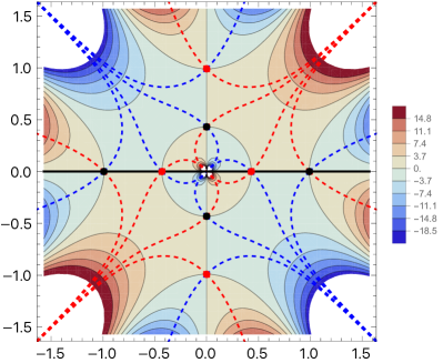
Figure 1: The contour plot of $\textrm{Re}\left[F(x)\right]$ over the complex $x$ plane for $\alpha=1$, $\beta=-3$, $\gamma=-0.1$, and $\hbar=1$, corresponding to the parameter region (i) $12\alpha\gamma+\beta^{2}>0$ with $\beta<0$. The black (red) circles represent the tunneling (no-boundary) saddle points while the blue (red) lines denote the (dual) Lefschetz thimbles. The black horizontal line denotes the original integration contour.

Let us study the thimble structures of the integral (8). As we will see soon, the structures are qualitatively different among the three parameter regions:

1. $12\alpha\gamma+\beta^{2}>0$ with $\beta<0$ ,

2. $12\alpha\gamma+\beta^{2}<0$ ,

3. $12\alpha\gamma+\beta^{2}>0$ with $\beta>0$ ,

where $12\alpha\gamma+\beta^{2}=V_{3}\left[q_{f}q_{i}\Lambda^{2}-3K\Lambda(q_{i}+q_{f})+9K^{2}\right]$. We note that the no-boundary and tunneling proposals set the parameters as $q_{i}=0$ and $K,\,\Lambda>0$ so that these correspond to regions (ii) and (iii). Fig. 1 shows the contour plot of $\textrm{Re}\left[F(x)\right]$ in Eq. (9) over the complex $x$ plane for $\alpha=1$, $\beta=-3$, $\gamma=-0.1$, and $\hbar=1$, which are representative values of the parameters in region (i). Note that the absolute value of $\hbar$ does not affect the thimble structures since it just changes the overall scaling of $F(x)$ while the phase of $\hbar$ turns out to be important as we will see later. From Fig. 1, we see that the four saddle points on the real axis contribute and the integral can be rewritten as a superposition of their thimbles unambiguously. Therefore, we can clearly say which saddles contribute in the case of the region (i) while we will see that the other cases are more intricate.

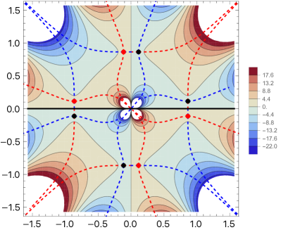
Figure 2: A similar plot to Fig. 1 with $\alpha=1$, $\beta=-3$, $\gamma=-1$ corresponding to the parameter region (ii) $12\alpha\gamma+\beta^{2}<0$. This corresponds to the no-boundary and tunneling proposals.

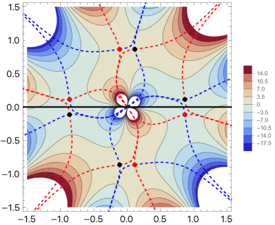
(a) $\theta=+\frac{\pi}{10}$

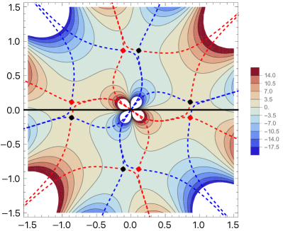
(b) $\theta=-\frac{\pi}{10}$

Figure 3: Complex deformation of Fig. 2 (in region (ii)) with $\hbar=e^{i\theta}$.

In Fig. 2, we show a similar plot to Fig. 1 in the parameter region (ii). A main difference from Fig. 1 is that some Lefschetz thimbles are passing two saddle points. This implies that we are on the Stokes lines and the decomposition (12) is ambiguous at the values of the parameters. In particular, we cannot judge how the no-boundary and tunneling saddle points contribute to the integral (8) just by Fig. 2. To see what is happening more precisely, we consider a deformation of the setup to go away from the Stokes lines. In particular, we take the expansion parameter $\hbar$ to be complex $e^{i\theta}$ as usually done in the context of resurgence. Fig. 3 shows similar plots to Fig. 2 but with nonzero $\theta$. Now we find that all the Lefschetz thimbles cross only one saddle point in contrast to the $\theta=0$ case in Fig. 2. Furthermore, the contributing saddle points are the same between $\theta>0$ and $\theta<0$: only the two tunneling saddles around the real axis contribute. This structure is maintained as long as $\theta$ is not strictly zero. The $\theta=0$ case of interest can be understood as the limit $\theta\rightarrow 0^{\pm}$ from nonzero $\theta$. The plots in Fig. 2 imply that the limit is smooth and independent of the directions of the limit. Therefore we conclude that the contributing saddles in the parameter region (ii) are the two tunneling saddles around the real axis. Our finding conclusively demonstrates that in traditional quantum cosmology, the tunneling proposal, rather than the no-boundary proposal, is the only approach that accurately describes the quantum creation of the universe from nothing.

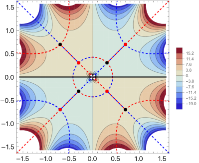
Figure 4: A similar plot to Figs. 1 and 2 with $\alpha=1$, $\beta=3$ and $\gamma=-0.1$ corresponding to region (iii) $12\alpha\gamma+\beta^{2}>0$ with $\beta>0$.

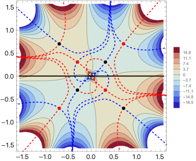
(a) $\theta=+\frac{\pi}{10}$

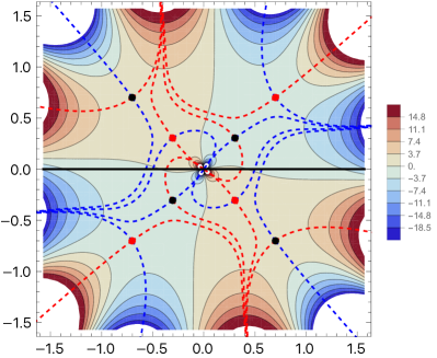
(b) $\theta=-\frac{\pi}{10}$

Figure 5: Complex deformation of Fig. 4 (in region (iii)) with $\hbar=e^{i\theta}$.

Let us turn to the parameter region (iii), whose thimble structure for $\theta=0$ is presented in Fig. 4. Again we see that some Lefschetz thimbles pass two saddle points and therefore we are on the Stokes lines. To resolve it, let us turn on the nonzero $\theta$ as in the region (ii) case. Fig. 5 shows similar plots to Fig. 4 for nonzero $\theta$, which are also similar to Fig. 3 but with a different parameter region. Here, all the Lefschetz thimbles cross only one saddle point as in the parameter region (ii) in Fig. 3. A main difference is that the contributing saddles are different between $\theta>0$ and $\theta<0$: all the four saddles in the first and third quadrants contribute for $\theta>0$ while only the two tunneling saddles in the quadrants contribute for $\theta<0$. This structure is maintained as long as $\theta$ is not strictly zero. This implies that the Stokes multipliers $n_{x_{s}}$ for the two no-boundary saddles in the quadrants introduced in Eq. (12) are like step functions jumping at $\theta=0$! Does this mean that the original integral itself (8) is discontinuous at $\theta=0$ ? We will see that the answer is no: although each term of the summand in Eq. (12) may be ambiguous due to a jump at $\theta=0$, the ambiguity is canceled from that coming from the other terms and then the whole answer is continuous. In other words, the limits $\theta\rightarrow 0^{+}$ and $\theta\rightarrow 0^{-}$ can be different for each term but are the same for the whole answer. It is known that this kind of cancellation typically happens in successful examples of the resurgence where ambiguities for Stokes multipliers of some saddles are canceled from ambiguities coming from the resummation of perturbative series around other saddles. In the next section, we will explicitly see the cancellations among the ambiguities coming from the Stokes multipliers of the two no-boundary saddles and the Borel resummation of the two tunneling saddles.

II.1 Comments on alternative integration range of lapse function

So far, we have considered the integration of the lapse function over $N\in(0,\infty)$ and this choice of $N$ ensures the causality [137]. On the other hand, considering all ranges of the lapse function $N\in(-\infty,\infty)$ is also possible [36, 37], which satisfies the gauge invariance of the lapse function. In this subsection, we comment on this case with all integration ranges of the lapse function $N\in(-\infty,\infty)$.

The authors of Refs. [36, 37] considered the deformation of the integration contour along the entire real axis to avoid singularities at the origin. In particular, they advocate the deformation into the lower half plane of $N$ to obtain the Hartle-Hawking no-boundary wave function. Let us compare their results with our discussion in terms of $x$ based on the resurgence technique. The integrand of $G(\hbar)$ (defined with the alternative contour) has a factor of $1/\sqrt{N}$ having a branch-cut singularity. When the contour of $N$ passes above the origin, the simplest path (without entering the second Riemann sheet) corresponds to the path of $x$ in the first quadrant asymptoting in the directions of the positive imaginary axis and the positive real axis. On the other hand, when the contour of $N$ passes below the origin, the simplest path corresponds to the path of $x$ in the third quadrant asymptoting in the directions of the negative imaginary axis and the positive real axis.

In the parameter region (i), the contour of $N$ avoiding the origin on the upper half plane is equivalent to the contour of $x$ composed of Lefschetz thimbles associated with both the no-boundary and tunneling saddle points on the positive imaginary axis and those on the positive real axis. The contour of $N$ avoiding the origin on the lower half plane is equivalent to the contour of $x$ composed of Lefschetz thimbles associated with the no-boundary saddle point on the negative imaginary axis and the tunneling saddle point on the positive real axis.

The parameter region (ii) is on the Stokes lines as we saw above. For the contour of $N$ avoiding the origin on the upper half plane, the contributing saddle points in terms of $x$ are the tunneling saddle points in the first quadrant for both signs of the deformation angle $\theta$. For the contour of $N$ avoiding the origin on the lower half plane, however, the contributing saddle points depend on the sign of the deformation angle $\theta$, in contrast to the analysis for only positive $N$. In particular, different tunneling saddles contribute for different signs of $\theta$ while the no boundary saddles contribute for both signs as seen from Fig. 3. Given this situation, it is unclear whether or not the $\theta\rightarrow 0^{\pm}$ limit of $G(\hbar)$ is real and satisfies the Wheeler-DeWitt equation. More detailed analysis is needed to have a clear answer.

The parameter region (iii) is also on the Stokes lines. For the contour of $N$ avoiding the origin on the upper half plane, the contributing saddle point in terms of $x$ is the no-boundary saddle point in the first quadrant for both signs of $\theta$. This is in contrast to the Stokes phenomenon found in the parameter region (iii) in the case of positive $N$. For the contour of $N$ avoiding the origin on the lower half plane, the contributing saddle points depend on the deformation angle $\theta$, signaling the Stokes phenomenon. See Fig. 5.

In this way, the ambiguity dependent on the original definition of the integration contour of $N$ remains as we work with $x$. This is not due to the insufficient power of our resurgence analyses, but rather, the different definitions of the original contour of $N$ simply correspond to inequivalent quantities.

III Resurgence analyses in Lorentzian quantum cosmology

In this section, we will apply the resurgence method to the Lorentzian path integral. For simplicity, we consider the persistence of spacetime where $q_{i}=q_{f}$ and the size of the universe does not change over time. In this case, we have $\gamma=0$, and obtain the following expression,

$$G(\hbar)=\sqrt{\frac{3iV_{3}}{4\pi}}\int^{\infty}_{-\infty}\mathrm{d}x\exp\left[i\left(\alpha\hbar^{2}x^{6}+\beta x^{2}\right)\right]\,,$$ (14)

where we transform $x\to x\sqrt{\hbar}$ and consider the integration range of $x$ from $-\infty$ to $+\infty$, for simplicity. There are five saddle points of the exponent,

$$x=0,\quad x_{i}=e^{\frac{i\arg\beta}{4}}e^{\frac{2n-1}{4}\pi i}\left(\frac{|\beta|}{3\alpha\hbar^{2}}\right)^{\frac{1}{4}}\quad(n=1,...,4),$$ (15)

where we take $\arg\beta=-\pi$ for $\beta<0$ such that $0\leq\arg{x_{i}}<2\pi$. From the viewpoint of the $\gamma\neq 0$ case, the trivial saddle $x=0$ comes from degeneration of four saddles out of the eight saddles in Eq. (10) which are $x_{n}^{+}$ with even (odd) $n$ and $x_{n}^{-}$ with odd (even) $n$ for $\beta>0$ ($\beta<0$).

Let us consider deriving the exact result from the perturbation expansion from the saddle points. First, we consider the contribution of the trivial saddle point, $x=0$:

$$\sqrt{\frac{3iV_{3}}{4\pi}}\int_{\mathcal{J}_{0}}\mathrm{d}x\exp\left[F\left(\sqrt{\hbar}x\right)\right],$$ (16)

and its small-$\hbar$ expansion formally given by

$$G_{0}(\hbar)=\sum_{n=0}^{\infty}c_{n}\hbar^{2n}\,.$$ (17)

To compute the perturbative coefficient $c_{n}$, we can replace the integral contour $\mathcal{J}_{0}$ with $(-e^{\pm\pi i/4}\infty,e^{\pm\pi i/4}\infty)$ for ${\rm sign}(\beta)=\pm 1$. Then the problem is reduced to integrals of polynomials of $x$ with the Gaussian weight and the coefficient $c_{n}$ is given by

$$c_{n}=e^{\pm\frac{\pi i}{4}}\sqrt{\frac{3iV_{3}}{4\pi|\beta|}}\cdot\frac{\Gamma(3n+\frac{1}{2})}{\Gamma(n+1)}\left(\frac{\alpha}{\beta^{3}}\right)^{n},$$ (18)

according to ${\rm sign}(\beta)=\pm 1$. As a result of the formal $\hbar$-expansion, it is found that Eq. (17) is an asymptotic series. Hence, we take its Borel resummation. As a first step of the resummation, we consider the Borel transformation ${\cal B}G_{0}(t)$ of Eq. (17). It is given by

$${\cal B}G_{0}(t)=\sum_{n=0}^{\infty}\frac{c_{n}}{\Gamma(2n+1)}t^{2n}\,.$$ (19)

This is a convergent series, and the infinite sum has an analytical expression for ${\rm sign}(\beta)=\pm 1$:

$${\cal B}G_{0}(t)=e^{\pm\frac{i\pi}{4}}\sqrt{\frac{3iV_{3}}{4|\beta|}}~{}_{2}F_{1}\left(\frac{1}{6},\frac{5}{6};1;\frac{27t^{2}\alpha}{4\beta^{3}}\right)\,,$$ (20)

where ${}_{2}F_{1}(a,b;c;z)$ is a hypergeometric function. We denote the Borel resummation of Eq. (14) as $\mathcal{S}_{\theta}G_{0}(\hbar)$, and it is defined by the Laplace transformation of Eq. (20):

$$\mathcal{S}_{\theta}G_{0}(\hbar)=\frac{1}{\hbar}\int_{0}^{\infty\cdot e^{i\theta}}\mathrm{d}t\,e^{-\frac{t}{\hbar}}{\cal B}G_{0}(t)\,,$$ (21)

where $\theta$ is the argument of $\hbar$.

For $\alpha>0$ and $\beta<0$, the Borel resummation $\mathcal{S}_{\theta}G_{0}(\hbar)$ is well-defined along $\theta=0$ and given by

$$\begin{split}\mathcal{S}_{0}G_{0}(\hbar)&=e^{-\frac{\pi i}{4}}\sqrt{\frac{3iV_{3}}{4}}\cdot\frac{\pi}{(12\alpha\hbar^{2})^{1/6}}\times\\ &\quad\left[\text{Ai}\left(\frac{\beta}{(12\alpha\hbar^{2})^{1/3}}\right)^{2}+\text{Bi}\left(\frac{\beta}{(12\alpha\hbar^{2})^{1/3}}\right)^{2}\right]\,,\end{split}$$ (22)

where $\text{Ai}(x)$ and $\text{Bi}(x)$ are Airy functions of the first and second kind, respectively.

For $\alpha>0$ and $\beta>0$, the Borel resummation $\mathcal{S}_{\theta}G_{0}(\hbar)$ along $\theta=0$ is not well-defined and non-Borel summable due to the branch cut of the hypergeometric function. One may try to make it well-defined by deforming the integral contour in Eq. (21) to avoid the branch cut, but then the value of the integral depends on how to avoid the branch cut. This ambiguity is estimated by the difference between the Borel resummations along the directions $\theta=0^{+}$ and $\theta=0^{-}$ as

$$\begin{split}&\left(\mathcal{S}_{0^{+}}-\mathcal{S}_{0^{-}}\right)G_{0}(\hbar)=\lim_{\epsilon\to 0}\frac{e^{\pi i/4}}{\hbar}\sqrt{\frac{3iV_{3}}{4\beta}}~{}\int_{t_{0}}^{\infty}\mathrm{d}t\,e^{-\frac{t}{\hbar}}\times\\ &\left[{}_{2}F_{1}\left(\frac{1}{6},\frac{5}{6};1;\frac{27t^{2}\alpha}{4\beta^{3}}+i\epsilon\right)-{}_{2}F_{1}\left(\frac{1}{6},\frac{5}{6};1;\frac{27t^{2}\alpha}{4\beta^{3}}-i\epsilon\right)\right]\\ &=\frac{e^{3\pi i/4}}{\hbar}\sqrt{\frac{3iV_{3}}{4\beta}}\int_{t_{0}}^{\infty}\mathrm{d}t\,e^{-\frac{t}{\hbar}}{}_{2}F_{1}\left(\frac{1}{6},\frac{5}{6};1;1-\frac{27t^{2}\alpha}{4\beta^{3}}\right)\,,\end{split}$$ (23)

where $t_{0}=(4\beta^{3}/27\alpha)^{1/2}$. As seen later, this ambiguity cancels the ambiguity of the Stokes multipliers for the no-boundary saddle points. To see the cancellation, we integrate Eq. (23) after $\hbar$-expansion of the integrand and obtain

$$\begin{split}&\left(\mathcal{S}_{0^{+}}-\mathcal{S}_{0^{-}}\right)G_{0}(\hbar)\\ &=e^{\frac{3\pi i}{4}}e^{-\frac{t_{0}}{\hbar}}\sqrt{\frac{3iV_{3}}{4\beta}}\left[1-\frac{5}{12}\left(\frac{3\alpha}{\beta^{3}}\right)^{1/2}\hbar+\mathcal{O}(\hbar^{2})\right].\end{split}$$ (24)

Next, we consider the contribution of the non-trivial saddle points, $x=x_{1}$ and $x_{3}$ for $\alpha>0$ and $\beta>0$. In this case, the angles of the steepest descent contours at the non-trivial saddle points are both $-\pi/4$. Hence, the contribution of the thimble associated with $x=x_{1}$ to the integral Eq. (14) is rewritten as

$$G(\hbar)|_{x=x_{1}} :=n_{x_{1}}\sqrt{\frac{3iV_{3}}{4\pi}}\int_{\mathcal{J}_{x_{1}}}\mathrm{d}x\exp\left[F\left(\sqrt{\hbar}x\right)\right]$$

$$=n_{x_{1}}e^{-\frac{\pi i}{4}}e^{-\frac{t_{0}}{\hbar}}\sqrt{\frac{3iV_{3}}{4\beta}}\int^{\infty}_{-\infty}{\rm d}\rho~{}e^{-4\beta\rho^{2}}e^{i\sigma_{1}(\rho)},$$ (25)

where we have substituted $x=x_{1}+\rho e^{-\pi i/4}$ and

$$\begin{split}\sigma_{1}(\rho)=&-20\left(\frac{\alpha\beta^{3}}{27}\right)^{1/4}\hbar^{1/2}\rho^{3}-5i(3\alpha\beta)^{1/2}\hbar\rho^{4}\\ &\quad+2(27\alpha^{3}\beta)^{1/4}\hbar^{3/2}\rho^{5}+i\alpha\hbar^{2}\rho^{6}.\end{split}$$ (26)

Integrating after $\hbar$-expansion of the integrand, we obtain

$$\begin{split}&G(\hbar)|_{x=x_{1}}\\ &=\frac{n_{x_{1}}}{2}e^{-\frac{\pi i}{4}}e^{-\frac{t_{0}}{\hbar}}\sqrt{\frac{3iV_{3}}{4\beta}}\left[1-\frac{5}{12}\left(\frac{3\alpha}{\beta^{3}}\right)^{1/2}\hbar+\mathcal{O}(\hbar^{2})\right].\end{split}$$ (27)

Since the contribution from the thimble passing through the saddle point $x=x_{3}$ is the same as that for $x=x_{1}$, we find the cancellation of the Borel ambiguity by the ambiguity of the Stokes multipliers for the nontrivial saddle points,

$$\left(\mathcal{S}_{0^{+}}\!-\mathcal{S}_{0^{-}}\right)G_{0}(\hbar)=-\!\!\!\!\!\!\sum_{x_{s}=x_{1},x_{3}}\!\!\!\!\!\left(G(\hbar)|_{x=x_{s}}^{\theta=0^{+}}\!-G(\hbar)|_{x=x_{s}}^{\theta=0^{-}}\right),$$ (28)

at the level of $\hbar$-expansion. We have analytically confirmed this cancellation up to the $100$th order of $\hbar$. In other words, the total $G(\hbar)$ in Eq. (14) is well-defined and continuous at $\theta=0$.

IV Neumann boundary condition and airy function

In the previous section, we have considered the Dirichlet boundary condition, which is a usual boundary condition. However, this boundary condition raises challenges regarding the stability of perturbations in Lorentzian quantum cosmology [140]. Although numerous studies and discussions have addressed this issue [36, 37, 141, 142, 143, 144, 145, 146, 147, 148, 149, 150, 151, 152], the only possible solution is to consider non-trivial boundary terms or conditions of the background geometry. There have been some works on Lorentzian quantum cosmology utilizing such non-trivial boundary conditions [149, 150, 31, 32, 33].

We consider the Neumann boundary condition. In general, it fixes $\dot{q}\mid_{t=t_{i}}$ and/or $\dot{q}\mid_{t=t_{f}}$, and the corresponding GHY term should be removed at $t=t_{i}$ and/or $t=t_{f}$. Since it has been pointed out that the Euclidean initial momentum is crucial for the success of the no-boundary proposal [149, 150], we impose the Neumann boundary condition at the initial time $t=t_{i}=0$. Imposing the Euclidean (imaginary) Neumann boundary conditions on the initial hypersurface, the perturbative instability can be avoided. Furthermore, the ambiguity of the contour of complex metrics can be removed.

Hereafter, we will consider the case imposing the Neumann boundary condition on the initial hypersurface and Dirichlet boundary condition on the final hypersurface,

$$-\frac{3\dot{q}(t_{i}=0)}{2N}=p_{i},\quad q(t_{f}=1)=q_{f},$$ (29)

where the canonical momentum is defined by $p=-\frac{3\dot{q}}{2N}$. With the action (3) and the above boundary condition, the path integral can be exactly evaluated, and we have the following expression [33],

$$G[q_{f};p_{i}] =\int_{-\infty}^{\infty}\mathrm{d}N\exp\biggl{[}\frac{iV_{3}}{\hbar}\biggl{\{}N\left(3K+\frac{p_{i}^{2}}{3}-\Lambda q_{f}\right)$$

$$+q_{f}p_{i}-\frac{1}{3}\Lambda p_{i}N^{2}+\frac{\Lambda^{2}N^{3}}{9}\biggr{\}}\biggr{]}\,,$$ (30)

where in the lapse integration, the absence of a pole means there is no ambiguity of the integration contours, unlike Section II. Additionally, the structure of the Lefschetz thimble remains consistent for both $N\in(0,\infty)$ and $N\in(-\infty,\infty)$. Thus, we consider the integration range of $N\in(0,\infty)$, for simplicity.

We will shift the lapse function $N=\bar{N}+\frac{p_{i}}{\Lambda}$ and this change reduces the transition amplitude to the following form,

$$G[q_{f};p_{i}] =\Psi(\hbar)\exp\left[\frac{iV_{3}}{\hbar}\frac{3}{\Lambda}\left(Kp_{i}+\frac{p_{i}^{3}}{27}\right)\right]\,,$$ (31)

where

$$\Psi(\hbar)\equiv\int_{-\infty}^{\infty}\mathrm{d}\bar{N}\exp\left[\frac{i}{\hbar}\left(\bar{\alpha}\bar{N}^{3}+\bar{\beta}\bar{N}\right)\right]\,,$$ (32)

with $\bar{\alpha}=\frac{V_{3}\Lambda^{2}}{9}$ and $\bar{\beta}=V_{3}\left(3K-\Lambda q_{f}\right)$. For instance, taking $p_{i}=0$, they describe the expansion of the universe from the de Sitter throat where $q(t=0)=3/\Lambda$ to a final hypersurface with $q(t=1)=q_{f}$, and the transition amplitude exactly takes the form of the Airy function. On the other hand, imposing the positively or negatively imaginary initial momentum $p_{i}=\pm 3i$, we can obtain the Hartle-Hawking no-boundary or the Vilenkin tunneling wave function, respectively, in a consistent way.

Although the Lefschetz thimble structure and resurgence analysis of the Airy functions are well-known, by examining these analytical properties of the Airy functions, we can re-evaluate the wave function in Lorentzian quantum cosmology. Now, by transforming $\bar{N}\to\bar{N}\sqrt{\hbar}$, we have the following expression,

$$\Psi(\hbar)=\int_{-\infty}^{\infty}\mathrm{d}\bar{N}\exp\left(i\bar{\alpha}\hbar^{2}\bar{N}^{3}+i\bar{\beta}\bar{N}\right)=\frac{2\pi\text{Ai}\left(\frac{\bar{\beta}}{\sqrt[3]{3\bar{\alpha}\hbar^{2}}}\right)}{\sqrt[3]{3\bar{\alpha}\hbar^{2}}}\,,$$ (33)

where we assume $\bar{\alpha},\,\bar{\beta}>0$ in the last equation. The action has two saddle points,

$$\bar{N}_{\pm}=\pm\frac{i}{\hbar}\sqrt{\frac{\bar{\beta}}{3\bar{\alpha}}}\,,$$ (34)

where we define $\bar{N}_{\pm}$ taking plus and minus sign, respectively. For $\bar{\alpha},\,\bar{\beta}>0$, we have two imaginary saddle points and consider this case for simplicity.

Now, we will consider the contributing saddle point $\bar{N}_{+}$, and evaluate $\Psi(\hbar)$ around this saddle point via the perturbative expansion. In this case, the Borel transform is given by

$${\cal B}\Psi_{+}(t)=\sum_{n=0}^{\infty}\frac{c_{n}}{\Gamma(\frac{n}{2}+1)}t^{\frac{n}{2}}\,,$$ (35)

where $c_{n}$ is given by

$$\begin{split}c_{n}=&\frac{(3\bar{\alpha}\bar{\beta}\hbar^{2})^{-\frac{1}{4}}}{2}e^{-\frac{2}{3\hbar}\sqrt{\frac{\bar{\beta}^{3}}{3\bar{\alpha}}}}\left((-1)^{3n}+1\right)\\ &\times\frac{\Gamma\left(\frac{3n}{2}+\frac{1}{2}\right)}{\Gamma(n+1)}\left(i\sqrt[4]{\frac{\bar{\alpha}}{27\bar{\beta}^{3}}}\right)^{n}.\end{split}$$ (36)

The Borel transform takes the analytical form,

$${\cal B}\Psi_{+}(t)=\sqrt[4]{\frac{\pi^{2}}{3\bar{\alpha}\bar{\beta}\hbar^{2}}}e^{-\frac{2}{3\hbar}\sqrt{\frac{\bar{\beta}^{3}}{3\bar{\alpha}}}}\,_{2}F_{1}\left(\frac{1}{6},\frac{5}{6};1;-\frac{3}{4}t\sqrt{\frac{3\bar{\alpha}}{\bar{\beta}^{3}}}\right)\,.$$ (37)

For $\bar{\alpha}>0$ and $\bar{\beta}>0$, the Borel transform has only one branch point along the negative real axis, and the Borel summation $\mathcal{S}_{\theta}\Psi_{+}(\hbar)$, where we take $\theta=0$, is

$$\begin{split}\mathcal{S}_{\theta}\Psi_{+}(\hbar)&=\frac{1}{\hbar}\int_{0}^{\infty\cdot e^{i\theta}}\mathrm{d}t\,e^{-\frac{t}{\hbar}}{\cal B}\Psi_{+}(t)\\ &=\frac{2\pi\text{Ai}\left(\frac{\bar{\beta}}{\sqrt[3]{3\bar{\alpha}\hbar^{2}}}\right)}{\sqrt[3]{3\bar{\alpha}\hbar^{2}}}\,,\end{split}$$ (38)

which is consistent with the result (33). Thus, we show that the perturbative expansion around the contributing saddle point is exactly consistent with the full integration. In Neumann and Robin boundary conditions, the Lefschetz thimble structures of quantum cosmology are trivial, and it is possible to accurately derive the wave function of the universe from the perturbative expansion around saddle points. This contrasts with the discussion of the Dirichlet conditions in Section III, where a detailed analysis is necessary to see the cancellation of the ambiguities of Borel resummation. In both cases, the wave function of the universe can be precisely derived with the resurgence theory.

V Conclusions

In this paper, we have studied the Lefschetz thimble structures and properties of quantum gravity corrections for the gravitational Lorentzian path integral. We have found that the thimble structures have qualitative differences among the three-parameter regions depending on the cosmological constant, extrinsic curvature, 3-dimensional volume factor, and boundary conditions.

In the region (i) $12\alpha\gamma+\beta^{2}>0$ with $\beta<0$, the integral is unambiguously decomposed into a superposition of the thimble integrals associated with the four real saddle points, where two of them are tunneling and the other two are no boundary ones.

In the region (ii) $12\alpha\gamma+\beta^{2}<0$, we are on the Stokes lines and the decomposition is ambiguous. To see what happens precisely, we have studied the thimble structures for complex $\hbar$ as usually done in the context of resurgence. Then, we have found that the complex case does not have ambiguities of the thimble decomposition and the structures are the same between $\theta>0$ and $\theta<0$. The $\theta=0$ case of interest can be understood as the limit $\theta\rightarrow 0^{\pm}$ from nonzero $\theta$. Therefore, we have concluded that the contributing saddles in the parameter region (ii) are the two tunneling saddles around the real axis. Our finding concludes that in traditional quantum cosmology, the tunneling wave function, rather than the no-boundary wave function accurately describes the quantum creation of the universe from nothing.

The case for the region (iii) $12\alpha\gamma+\beta^{2}>0$ with $\beta>0$ is also on Stokes lines. However, we have found a difference that the contributing saddles are different between $\theta>0$ and $\theta<0$: all four saddles in the first and third quadrants contribute for $\theta>0$ while only the two tunneling saddles in the quadrants contribute for $\theta<0$. This implies that the Stokes multipliers for the two no-boundary saddles are like step functions jumping at $\theta=0$. We have found that although each term of the summand may be ambiguous due to a jump at $\theta=0$, the ambiguity is canceled from that coming from the other terms, and then the whole answer is continuous. We have explicitly demonstrated the cancellations among the ambiguities coming from the Stokes multipliers of the two no-boundary saddles and the Borel resummation of the two tunneling saddles.

For the Neumann and Robin boundary conditions, the Lefschetz thimble structures in quantum cosmology are trivial, reducing the gravitational path integral to the form of Airy functions. Consequently, deriving the no-boundary or tunneling wave function from the perturbative expansion around saddle points becomes straightforward.

This study demonstrates that applying resurgence theory to the Lorentzian quantum cosmology framework allows for a consistent derivation of the wave function of the universe. Exploring the Lefschetz-thimble and resurgence structures in other models of quantum cosmology would be interesting.

References

- [1] S. W. Hawking, “Quantum Gravity and Path Integrals,” Phys. Rev. D 18 (1978) 1747–1753.
- [2] J. B. Hartle and S. W. Hawking, “Wave Function of the Universe,” Phys. Rev. D 28 (1983) 2960–2975.
- [3] A. Vilenkin, “Creation of Universes from Nothing,” Phys. Lett. B 117 (1982) 25–28.
- [4] G. W. Gibbons, S. W. Hawking, and M. J. Perry, “Path Integrals and the Indefiniteness of the Gravitational Action,” Nucl. Phys. B 138 (1978) 141–150.
- [5] A. D. Linde, “Quantum Creation of the Inflationary Universe,” Lett. Nuovo Cim. 39 (1984) 401–405.
- [6] J. J. Halliwell and J. Louko, “Steepest Descent Contours in the Path Integral Approach to Quantum Cosmology. 1. The De Sitter Minisuperspace Model,” Phys. Rev. D 39 (1989) 2206.
- [7] A. Vilenkin, “Quantum Creation of Universes,” Phys. Rev. D 30 (1984) 509–511.
- [8] A. D. Linde, “Quantum creation of an inflationary universe,” Sov. Phys. JETP 60 (1984) 211–213.
- [9] A. D. Linde, “The Inflationary Universe,” Rept. Prog. Phys. 47 (1984) 925–986.
- [10] V. A. Rubakov, “Quantum Mechanics in the Tunneling Universe,” Phys. Lett. B 148 (1984) 280–286.
- [11] Y. B. Zeldovich and A. A. Starobinsky, “Quantum creation of a universe in a nontrivial topology,” Sov. Astron. Lett. 10 (1984) 135.
- [12] A. Vilenkin, “Boundary Conditions in Quantum Cosmology,” Phys. Rev. D 33 (1986) 3560.
- [13] A. Vilenkin, “Quantum Cosmology and the Initial State of the Universe,” Phys. Rev. D 37 (1988) 888.
- [14] J. Feldbrugge, J.-L. Lehners, and N. Turok, “Lorentzian Quantum Cosmology,” Phys. Rev. D 95 no. 10, (2017) 103508, arXiv:1703.02076 [hep-th].
- [15] F. PHAM, “Vanishing homologies and the n variables saddlepoint method,” Proc. Symp. Pure Math. 40 (1983) 310–333.
- [16] M. V. Berry and C. J. Howls, “Hyperasymptotics for integrals with saddles,” Proceedings: Mathematical and Physical Sciences 434 no. 1892, (1991) 657–675.
- [17] C. J. Howls, “Hyperasymptotics for multidimensional integrals, exact remainder terms and the global connection problem,” Proceedings of the Royal Society of London. Series A: Mathematical, Physical and Engineering Sciences 453 no. 1966, (1997) 2271–2294.
- [18] E. Witten, “Analytic Continuation Of Chern-Simons Theory,” AMS/IP Stud. Adv. Math. 50 (2011) 347–446, arXiv:1001.2933 [hep-th].
- [19] Z.-G. Mou, P. M. Saffin, A. Tranberg, and S. Woodward, “Real-time quantum dynamics, path integrals and the method of thimbles,” JHEP 06 (2019) 094, arXiv:1902.09147 [hep-lat].
- [20] Z.-G. Mou, P. M. Saffin, and A. Tranberg, “Quantum tunnelling, real-time dynamics and Picard-Lefschetz thimbles,” JHEP 11 (2019) 135, arXiv:1909.02488 [hep-th].
- [21] P. Millington, Z.-G. Mou, P. M. Saffin, and A. Tranberg, “Statistics on Lefschetz thimbles: Bell/Leggett-Garg inequalities and the classical-statistical approximation,” JHEP 03 (2021) 077, arXiv:2011.02657 [hep-th].
- [22] H. Matsui, “Lorentzian path integral for quantum tunneling and WKB approximation for wave-function,” Eur. Phys. J. C 82 no. 5, (2022) 426, arXiv:2102.09767 [gr-qc].
- [23] K. Rajeev, “Lorentzian worldline path integral approach to Schwinger effect,” Phys. Rev. D 104 no. 10, (2021) 105014, arXiv:2105.12194 [hep-th].
- [24] T. Hayashi, K. Kamada, N. Oshita, and J. Yokoyama, “Vacuum decay in the Lorentzian path integral,” JCAP 05 no. 05, (2022) 041, arXiv:2112.09284 [hep-th].
- [25] J. Feldbrugge and N. Turok, “Existence of real time quantum path integrals,” Annals Phys. 454 (2023) 169315, arXiv:2207.12798 [hep-th].
- [26] J. Nishimura, K. Sakai, and A. Yosprakob, “A new picture of quantum tunneling in the real-time path integral from Lefschetz thimble calculations,” JHEP 09 (2023) 110, arXiv:2307.11199 [hep-th].
- [27] J. Feldbrugge, D. L. Jow, and U.-L. Pen, “Complex classical paths in quantum reflections and tunneling,” arXiv:2309.12420 [quant-ph].
- [28] J. Feldbrugge, D. L. Jow, and U.-L. Pen, “Crossing singularities in the saddle point approximation,” arXiv:2309.12427 [quant-ph].
- [29] R. L. Arnowitt, S. Deser, and C. W. Misner, “The Dynamics of general relativity,” Gen. Rel. Grav. 40 (2008) 1997–2027, arXiv:gr-qc/0405109.
- [30] G. Fanaras and A. Vilenkin, “Jackiw-Teitelboim and Kantowski-Sachs quantum cosmology,” JCAP 03 no. 03, (2022) 056, arXiv:2112.00919 [gr-qc].
- [31] G. Narain, “On Gauss-bonnet gravity and boundary conditions in Lorentzian path-integral quantization,” JHEP 05 (2021) 273, arXiv:2101.04644 [gr-qc].
- [32] G. Narain, “Surprises in Lorentzian path-integral of Gauss-Bonnet gravity,” JHEP 04 (2022) 153, arXiv:2203.05475 [gr-qc].
- [33] M. Ailiga, S. Mallik, and G. Narain, “Lorentzian Robin Universe,” JHEP 01 (2024) 124, arXiv:2308.01310 [gr-qc].
- [34] J.-L. Lehners, “Review of the no-boundary wave function,” Phys. Rept. 1022 (2023) 1–82, arXiv:2303.08802 [hep-th].
- [35] H. Matsui and S. Mukohyama, “Hartle-Hawking no-boundary proposal and Hořava-Lifshitz gravity,” Phys. Rev. D 109 no. 2, (2024) 023504, arXiv:2310.00210 [gr-qc].
- [36] J. Diaz Dorronsoro, J. J. Halliwell, J. B. Hartle, T. Hertog, and O. Janssen, “Real no-boundary wave function in Lorentzian quantum cosmology,” Phys. Rev. D 96 no. 4, (2017) 043505, arXiv:1705.05340 [gr-qc].
- [37] J. Feldbrugge, J.-L. Lehners, and N. Turok, “No rescue for the no boundary proposal: Pointers to the future of quantum cosmology,” Phys. Rev. D 97 no. 2, (2018) 023509, arXiv:1708.05104 [hep-th].
- [38] J. Ecalle, “Un analogue des fonctions automorphes : les fonctions résurgentes,” Séminaire Choquet. Initiation à l’analyse 17 no. 1, (1977-1978) . talk:11.
- [39] O. Costin, Asymptotics and Borel summability. Monographs and Surveys in Pure and Applied Mathematics. CRC Press, Hoboken, NJ, 2008.
- [40] M. Marino, “Lectures on non-perturbative effects in large N gauge theories, matrix models and strings,” arXiv:1206.6272 [hep-th].
- [41] D. Dorigoni, “An Introduction to Resurgence, Trans-Series and Alien Calculus,” Annals Phys. 409 (2019) 167914, arXiv:1411.3585 [hep-th].
- [42] I. Aniceto, G. Başar, and R. Schiappa, “A primer on resurgent transseries and their asymptotics,” Physics Reports 809 (2019) 1–135.
- [43] D. Sauzin, “Introduction to 1-summability and resurgence,” arXiv:1405.0356 [math.DS].
- [44] M. Marino, R. Schiappa, and M. Weiss, “Multi-Instantons and Multi-Cuts,” J. Math. Phys. 50 (2009) 052301, arXiv:0809.2619 [hep-th].
- [45] S. Garoufalidis, A. Its, A. Kapaev, and M. Marino, “Asymptotics of the instantons of Painlevé I,” Int. Math. Res. Not. 2012 no. 3, (2012) 561–606, arXiv:1002.3634 [math.CA].
- [46] C.-T. Chan, H. Irie, and C.-H. Yeh, “Stokes Phenomena and Non-perturbative Completion in the Multi-cut Two-matrix Models,” Nucl. Phys. B 854 (2012) 67–132, arXiv:1011.5745 [hep-th].
- [47] C.-T. Chan, H. Irie, and C.-H. Yeh, “Stokes Phenomena and Quantum Integrability in Non-critical String/M Theory,” Nucl. Phys. B 855 (2012) 46–81, arXiv:1109.2598 [hep-th].
- [48] R. Schiappa and R. Vaz, “The Resurgence of Instantons: Multi-Cut Stokes Phases and the Painleve II Equation,” Commun. Math. Phys. 330 (2014) 655–721, arXiv:1302.5138 [hep-th].
- [49] M. Marino, “Open string amplitudes and large order behavior in topological string theory,” JHEP 03 (2008) 060, arXiv:hep-th/0612127.
- [50] M. Marino, R. Schiappa, and M. Weiss, “Nonperturbative Effects and the Large-Order Behavior of Matrix Models and Topological Strings,” Commun. Num. Theor. Phys. 2 (2008) 349–419, arXiv:0711.1954 [hep-th].
- [51] M. Marino, “Nonperturbative effects and nonperturbative definitions in matrix models and topological strings,” JHEP 12 (2008) 114, arXiv:0805.3033 [hep-th].
- [52] S. Pasquetti and R. Schiappa, “Borel and Stokes Nonperturbative Phenomena in Topological String Theory and c=1 Matrix Models,” Annales Henri Poincare 11 (2010) 351–431, arXiv:0907.4082 [hep-th].
- [53] I. Aniceto, R. Schiappa, and M. Vonk, “The Resurgence of Instantons in String Theory,” Commun. Num. Theor. Phys. 6 (2012) 339–496, arXiv:1106.5922 [hep-th].
- [54] R. Couso-Santamaría, J. D. Edelstein, R. Schiappa, and M. Vonk, “Resurgent Transseries and the Holomorphic Anomaly,” Annales Henri Poincare 17 no. 2, (2016) 331–399, arXiv:1308.1695 [hep-th].
- [55] R. Couso-Santamaría, J. D. Edelstein, R. Schiappa, and M. Vonk, “Resurgent Transseries and the Holomorphic Anomaly: Nonperturbative Closed Strings in Local ,” Commun. Math. Phys. 338 no. 1, (2015) 285–346, arXiv:1407.4821 [hep-th].
- [56] A. Grassi, M. Marino, and S. Zakany, “Resumming the string perturbation series,” JHEP 05 (2015) 038, arXiv:1405.4214 [hep-th].
- [57] R. Couso-Santamaría, R. Schiappa, and R. Vaz, “Finite N from Resurgent Large N,” Annals Phys. 356 (2015) 1–28, arXiv:1501.01007 [hep-th].
- [58] R. Couso-Santamaría, R. Schiappa, and R. Vaz, “On asymptotics and resurgent structures of enumerative Gromov–Witten invariants,” Commun. Num. Theor. Phys. 11 (2017) 707–790, arXiv:1605.07473 [math.AG].
- [59] R. Couso-Santamaría, M. Marino, and R. Schiappa, “Resurgence Matches Quantization,” J. Phys. A 50 no. 14, (2017) 145402, arXiv:1610.06782 [hep-th].
- [60] T. Kuroki and F. Sugino, “Resurgence of one-point functions in a matrix model for 2D type IIA superstrings,” JHEP 05 (2019) 138, arXiv:1901.10349 [hep-th].
- [61] T. Kuroki, “Two-point functions at arbitrary genus and its resurgence structure in a matrix model for 2D type IIA superstrings,” JHEP 07 (2020) 118, arXiv:2004.13346 [hep-th].
- [62] D. Dorigoni, A. Kleinschmidt, and R. Treilis, “To the cusp and back: resurgent analysis for modular graph functions,” JHEP 11 (2022) 048, arXiv:2208.14087 [hep-th].
- [63] S. Baldino, R. Schiappa, M. Schwick, and R. Vega, “Resurgent Stokes data for Painlevé equations and two-dimensional quantum (super) gravity,” Commun. Num. Theor. Phys. 17 no. 2, (2023) 385–552, arXiv:2203.13726 [hep-th].
- [64] R. Schiappa, M. Schwick, and N. Tamarin, “All the D-Branes of Resurgence,” arXiv:2301.05214 [hep-th].
- [65] K. Iwaki and M. Marino, “Resurgent Structure of the Topological String and the First Painlevé Equation,” arXiv:2307.02080 [hep-th].
- [66] S. Alexandrov, M. Marino, and B. Pioline, “Resurgence of refined topological strings and dual partition functions,” arXiv:2311.17638 [hep-th].
- [67] I. Aniceto and M. Spaliński, “Resurgence in Extended Hydrodynamics,” Phys. Rev. D 93 no. 8, (2016) 085008, arXiv:1511.06358 [hep-th].
- [68] G. Basar and G. V. Dunne, “Hydrodynamics, resurgence, and transasymptotics,” Phys. Rev. D 92 no. 12, (2015) 125011, arXiv:1509.05046 [hep-th].
- [69] J. Casalderrey-Solana, N. I. Gushterov, and B. Meiring, “Resurgence and Hydrodynamic Attractors in Gauss-Bonnet Holography,” JHEP 04 (2018) 042, arXiv:1712.02772 [hep-th].
- [70] A. Behtash, C. N. Cruz-Camacho, and M. Martinez, “Far-from-equilibrium attractors and nonlinear dynamical systems approach to the Gubser flow,” Phys. Rev. D 97 no. 4, (2018) 044041, arXiv:1711.01745 [hep-th].
- [71] M. P. Heller and V. Svensson, “How does relativistic kinetic theory remember about initial conditions?,” Phys. Rev. D 98 no. 5, (2018) 054016, arXiv:1802.08225 [nucl-th].
- [72] M. P. Heller, A. Serantes, M. Spaliński, V. Svensson, and B. Withers, “The hydrodynamic gradient expansion in linear response theory,” arXiv:2007.05524 [hep-th].
- [73] I. Aniceto, B. Meiring, J. Jankowski, and M. Spaliński, “The large proper-time expansion of Yang-Mills plasma as a resurgent transseries,” JHEP 02 (2019) 073, arXiv:1810.07130 [hep-th].
- [74] A. Behtash, S. Kamata, M. Martinez, T. Schäfer, and V. Skokov, “Transasymptotics and hydrodynamization of the Fokker-Planck equation for gluons,” Phys. Rev. D 103 no. 5, (2021) 056010, arXiv:2011.08235 [hep-ph].
- [75] L. Griguolo, R. Panerai, J. Papalini, and D. Seminara, “Nonperturbative effects and resurgence in Jackiw-Teitelboim gravity at finite cutoff,” Phys. Rev. D 105 no. 4, (2022) 046015, arXiv:2106.01375 [hep-th].
- [76] P. Gregori and R. Schiappa, “From Minimal Strings towards Jackiw-Teitelboim Gravity: On their Resurgence, Resonance, and Black Holes,” arXiv:2108.11409 [hep-th].
- [77] B. Eynard, E. Garcia-Failde, P. Gregori, D. Lewanski, and R. Schiappa, “Resurgent Asymptotics of Jackiw-Teitelboim Gravity and the Nonperturbative Topological Recursion,” arXiv:2305.16940 [hep-th].
- [78] G. V. Dunne and M. Unsal, “Resurgence and Trans-series in Quantum Field Theory: The CP(N-1) Model,” JHEP 11 (2012) 170, arXiv:1210.2423 [hep-th].
- [79] G. V. Dunne and M. Unsal, “Continuity and Resurgence: towards a continuum definition of the (N-1) model,” Phys. Rev. D87 (2013) 025015, arXiv:1210.3646 [hep-th].
- [80] A. Cherman, D. Dorigoni, G. V. Dunne, and M. Unsal, “Resurgence in Quantum Field Theory: Nonperturbative Effects in the Principal Chiral Model,” Phys. Rev. Lett. 112 (2014) 021601, arXiv:1308.0127 [hep-th].
- [81] A. Cherman, D. Dorigoni, and M. Unsal, “Decoding perturbation theory using resurgence: Stokes phenomena, new saddle points and Lefschetz thimbles,” JHEP 10 (2015) 056, arXiv:1403.1277 [hep-th].
- [82] T. Misumi, M. Nitta, and N. Sakai, “Neutral bions in the model,” JHEP 06 (2014) 164, arXiv:1404.7225 [hep-th].
- [83] A. Behtash, T. Sulejmanpasic, T. Schäfer, and M. Ünsal, “Hidden topological angles and Lefschetz thimbles,” Phys. Rev. Lett. 115 no. 4, (2015) 041601, arXiv:1502.06624 [hep-th].
- [84] G. V. Dunne and M. Unsal, “Resurgence and Dynamics of O(N) and Grassmannian Sigma Models,” JHEP 09 (2015) 199, arXiv:1505.07803 [hep-th].
- [85] P. V. Buividovich, G. V. Dunne, and S. N. Valgushev, “Complex Path Integrals and Saddles in Two-Dimensional Gauge Theory,” Phys. Rev. Lett. 116 no. 13, (2016) 132001, arXiv:1512.09021 [hep-th].
- [86] S. Demulder, D. Dorigoni, and D. C. Thompson, “Resurgence in -deformed Principal Chiral Models,” JHEP 07 (2016) 088, arXiv:1604.07851 [hep-th].
- [87] K. Okuyama and K. Sakai, “Resurgence analysis of 2d Yang-Mills theory on a torus,” JHEP 08 (2018) 065, arXiv:1806.00189 [hep-th].
- [88] M. Mariño and T. Reis, “Renormalons in integrable field theories,” JHEP 04 (2020) 160, arXiv:1909.12134 [hep-th].
- [89] M. Mariño and T. Reis, “A new renormalon in two dimensions,” JHEP 07 (2020) 216, arXiv:1912.06228 [hep-th].
- [90] M. C. Abbott, Z. Bajnok, J. Balog, A. Hegedús, and S. Sadeghian, “Resurgence in the O(4) sigma model,” arXiv:2011.12254 [hep-th].
- [91] M. C. Abbott, Z. Bajnok, J. Balog, and A. Hegedús, “From perturbative to non-perturbative in the O(4) sigma model,” arXiv:2011.09897 [hep-th].
- [92] M. Marino, R. Miravitllas, and T. Reis, “Testing the Bethe ansatz with large N renormalons,” Eur. Phys. J. ST 230 no. 12-13, (2021) 2641–2666, arXiv:2102.03078 [hep-th].
- [93] L. Di Pietro, M. Mariño, G. Sberveglieri, and M. Serone, “Resurgence and 1/N Expansion in Integrable Field Theories,” JHEP 10 (2021) 166, arXiv:2108.02647 [hep-th].
- [94] M. Marino, R. Miravitllas, and T. Reis, “New renormalons from analytic trans-series,” JHEP 08 (2022) 279, arXiv:2111.11951 [hep-th].
- [95] M. Marino, R. Miravitllas, and T. Reis, “Instantons, renormalons and the theta angle in integrable sigma models,” SciPost Phys. 15 no. 5, (2023) 184, arXiv:2205.04495 [hep-th].
- [96] T. Reis, On the resurgence of renormalons in integrable theories. PhD thesis, U. Geneva (main), 2022. arXiv:2209.15386 [hep-th].
- [97] M. Marino, R. Miravitllas, and T. Reis, “On the structure of trans-series in quantum field theory,” arXiv:2302.08363 [hep-th].
- [98] S. Gukov, M. Marino, and P. Putrov, “Resurgence in complex Chern-Simons theory,” arXiv:1605.07615 [hep-th].
- [99] D. Gang and Y. Hatsuda, “S-duality resurgence in SL(2) Chern-Simons theory,” JHEP 07 (2018) 053, arXiv:1710.09994 [hep-th].
- [100] D. H. Wu, “Resurgent analysis of SU(2) Chern-Simons partition function on Brieskorn spheres ,” JHEP 21 (2020) 008, arXiv:2010.13736 [hep-th].
- [101] F. Ferrari and P. Putrov, “Supergroups, q-series and 3-manifolds,” arXiv:2009.14196 [hep-th].
- [102] S. Gukov and C. Manolescu, “A two-variable series for knot complements,” arXiv:1904.06057 [math.GT].
- [103] S. Garoufalidis, J. Gu, and M. Marino, “The resurgent structure of quantum knot invariants,” arXiv:2007.10190 [hep-th].
- [104] H. Fuji, K. Iwaki, H. Murakami, and Y. Terashima, “Witten-Reshetikhin-Turaev function for a knot in Seifert manifolds,” arXiv:2007.15872 [math.GT].
- [105] S. Garoufalidis, J. Gu, M. Marino, and C. Wheeler, “Resurgence of Chern-Simons theory at the trivial flat connection,” arXiv:2111.04763 [math.GT].
- [106] N. Dondi, I. Kalogerakis, D. Orlando, and S. Reffert, “Resurgence of the large-charge expansion,” arXiv:2102.12488 [hep-th].
- [107] P. Argyres and M. Unsal, “A semiclassical realization of infrared renormalons,” Phys. Rev. Lett. 109 (2012) 121601, arXiv:1204.1661 [hep-th].
- [108] G. V. Dunne, M. Shifman, and M. Unsal, “Infrared Renormalons versus Operator Product Expansions in Supersymmetric and Related Gauge Theories,” Phys. Rev. Lett. 114 no. 19, (2015) 191601, arXiv:1502.06680 [hep-th].
- [109] H. Mera, T. G. Pedersen, and B. K. Nikolić, “Fast summation of divergent series and resurgent transseries from Meijer- G approximants,” Phys. Rev. D 97 no. 10, (2018) 105027, arXiv:1802.06034 [hep-th].
- [110] F. Canfora, M. Lagos, S. H. Oh, J. Oliva, and A. Vera, “Analytic (3+1)-dimensional gauged Skyrmions, Heun, and Whittaker-Hill equations and resurgence,” Phys. Rev. D 98 no. 8, (2018) 085003, arXiv:1809.10386 [hep-th].
- [111] M. Ünsal, “Strongly coupled QFT dynamics via TQFT coupling,” arXiv:2007.03880 [hep-th].
- [112] M. Borinsky, G. V. Dunne, and M. Meynig, “Semiclassical Trans-Series from the Perturbative Hopf-Algebraic Dyson-Schwinger Equations: QFT in 6 Dimensions,” SIGMA 17 (2021) 087, arXiv:2104.00593 [hep-th].
- [113] M. Borinsky and D. Broadhurst, “Resonant resurgent asymptotics from quantum field theory,” Nucl. Phys. B 981 (2022) 115861, arXiv:2202.01513 [hep-th].
- [114] J. G. Russo, “A Note on perturbation series in supersymmetric gauge theories,” JHEP 06 (2012) 038, arXiv:1203.5061 [hep-th].
- [115] I. Aniceto, J. G. Russo, and R. Schiappa, “Resurgent Analysis of Localizable Observables in Supersymmetric Gauge Theories,” JHEP 03 (2015) 172, arXiv:1410.5834 [hep-th].
- [116] I. Aniceto, “The Resurgence of the Cusp Anomalous Dimension,” J. Phys. A 49 (2016) 065403, arXiv:1506.03388 [hep-th].
- [117] M. Honda, “Borel Summability of Perturbative Series in 4D and 5D =1 Supersymmetric Theories,” Phys. Rev. Lett. 116 no. 21, (2016) 211601, arXiv:1603.06207 [hep-th].
- [118] M. Honda, “How to resum perturbative series in 3d N=2 Chern-Simons matter theories,” Phys. Rev. D94 no. 2, (2016) 025039, arXiv:1604.08653 [hep-th].
- [119] M. Honda, “Role of Complexified Supersymmetric Solutions,” arXiv:1710.05010 [hep-th].
- [120] S. Gukov, D. Pei, P. Putrov, and C. Vafa, “BPS spectra and 3-manifold invariants,” J. Knot Theor. Ramifications 29 no. 02, (2020) 2040003, arXiv:1701.06567 [hep-th].
- [121] D. Dorigoni and P. Glass, “The grin of Cheshire cat resurgence from supersymmetric localization,” SciPost Phys. 4 no. 2, (2018) 012, arXiv:1711.04802 [hep-th].
- [122] M. Honda and D. Yokoyama, “Resumming perturbative series in the presence of monopole bubbling effects,” Phys. Rev. D 100 no. 2, (2019) 025012, arXiv:1711.10799 [hep-th].
- [123] T. Fujimori, M. Honda, S. Kamata, T. Misumi, and N. Sakai, “Resurgence and Lefschetz thimble in three-dimensional supersymmetric Chern–Simons matter theories,” PTEP 2018 no. 12, (2018) 123B03, arXiv:1805.12137 [hep-th].
- [124] A. Grassi, J. Gu, and M. Mariño, “Non-perturbative approaches to the quantum Seiberg-Witten curve,” JHEP 07 (2020) 106, arXiv:1908.07065 [hep-th].
- [125] D. Dorigoni and P. Glass, “Picard-Lefschetz decomposition and Cheshire Cat resurgence in 3D = 2 field theories,” JHEP 12 (2019) 085, arXiv:1909.05262 [hep-th].
- [126] D. Dorigoni, M. B. Green, and C. Wen, “Exact properties of an integrated correlator in SYM,” arXiv:2102.09537 [hep-th].
- [127] T. Fujimori, M. Honda, S. Kamata, T. Misumi, N. Sakai, and T. Yoda, “Quantum phase transition and resurgence: Lessons from three-dimensional supersymmetric quantum electrodynamics,” PTEP 2021 no. 10, (2021) 103B04, arXiv:2103.13654 [hep-th].
- [128] M. Beccaria, G. V. Dunne, and A. A. Tseytlin, “Strong coupling expansion of free energy and BPS Wilson loop in = 2 superconformal models with fundamental hypermultiplets,” JHEP 08 (2021) 102, arXiv:2105.14729 [hep-th].
- [129] Y. Hatsuda and M. Kimura, “Spectral Problems for Quasinormal Modes of Black Holes,” Universe 7 no. 12, (2021) 476, arXiv:2111.15197 [gr-qc].
- [130] Y. Hatsuda, “Quasinormal modes of black holes and Borel summation,” Phys. Rev. D 101 no. 2, (2020) 024008, arXiv:1906.07232 [gr-qc].
- [131] J. Matyjasek and M. Telecka, “Quasinormal modes of black holes. II. Padé summation of the higher-order WKB terms,” Phys. Rev. D 100 no. 12, (2019) 124006, arXiv:1908.09389 [gr-qc].
- [132] D. S. Eniceicu and M. Reece, “Quasinormal modes of charged fields in Reissner-Nordström backgrounds by Borel-Padé summation of Bender-Wu series,” Phys. Rev. D 102 no. 4, (2020) 044015, arXiv:1912.05553 [gr-qc].
- [133] M. Honda, R. Jinno, L. Pinol, and K. Tokeshi, “Borel resummation of secular divergences in stochastic inflation,” JHEP 08 (2023) 060, arXiv:2304.02592 [hep-th].
- [134] E. S. Fradkin and G. A. Vilkovisky, “QUANTIZATION OF RELATIVISTIC SYSTEMS WITH CONSTRAINTS,” Phys. Lett. B 55 (1975) 224–226.
- [135] I. A. Batalin and G. A. Vilkovisky, “Relativistic S Matrix of Dynamical Systems with Boson and Fermion Constraints,” Phys. Lett. B 69 (1977) 309–312.
- [136] J. J. Halliwell, “Derivation of the Wheeler-De Witt Equation from a Path Integral for Minisuperspace Models,” Phys. Rev. D 38 (1988) 2468.
- [137] C. Teitelboim, “Causality Versus Gauge Invariance in Quantum Gravity and Supergravity,” Phys. Rev. Lett. 50 (1983) 705.
- [138] T. Kanazawa and Y. Tanizaki, “Structure of Lefschetz thimbles in simple fermionic systems,” JHEP 03 (2015) 044, arXiv:1412.2802 [hep-th].
- [139] H. Fujii, S. Kamata, and Y. Kikukawa, “Monte Carlo study of Lefschetz thimble structure in one-dimensional Thirring model at finite density,” JHEP 12 (2015) 125, arXiv:1509.09141 [hep-lat]. [Erratum: JHEP 09, 172 (2016)].
- [140] J. Feldbrugge, J.-L. Lehners, and N. Turok, “No smooth beginning for spacetime,” Phys. Rev. Lett. 119 no. 17, (2017) 171301, arXiv:1705.00192 [hep-th].
- [141] J. Feldbrugge, J.-L. Lehners, and N. Turok, “Inconsistencies of the New No-Boundary Proposal,” Universe 4 no. 10, (2018) 100, arXiv:1805.01609 [hep-th].
- [142] J. Diaz Dorronsoro, J. J. Halliwell, J. B. Hartle, T. Hertog, O. Janssen, and Y. Vreys, “Damped perturbations in the no-boundary state,” Phys. Rev. Lett. 121 no. 8, (2018) 081302, arXiv:1804.01102 [gr-qc].
- [143] J. J. Halliwell, J. B. Hartle, and T. Hertog, “What is the No-Boundary Wave Function of the Universe?,” Phys. Rev. D 99 no. 4, (2019) 043526, arXiv:1812.01760 [hep-th].
- [144] O. Janssen, J. J. Halliwell, and T. Hertog, “No-boundary proposal in biaxial Bianchi IX minisuperspace,” Phys. Rev. D 99 no. 12, (2019) 123531, arXiv:1904.11602 [gr-qc].
- [145] A. Vilenkin and M. Yamada, “Tunneling wave function of the universe,” Phys. Rev. D 98 no. 6, (2018) 066003, arXiv:1808.02032 [gr-qc].
- [146] A. Vilenkin and M. Yamada, “Tunneling wave function of the universe II: the backreaction problem,” Phys. Rev. D 99 no. 6, (2019) 066010, arXiv:1812.08084 [gr-qc].
- [147] M. Bojowald and S. Brahma, “Loops rescue the no-boundary proposal,” Phys. Rev. Lett. 121 no. 20, (2018) 201301, arXiv:1810.09871 [gr-qc].
- [148] A. Di Tucci and J.-L. Lehners, “Unstable no-boundary fluctuations from sums over regular metrics,” Phys. Rev. D 98 no. 10, (2018) 103506, arXiv:1806.07134 [gr-qc].
- [149] A. Di Tucci and J.-L. Lehners, “No-Boundary Proposal as a Path Integral with Robin Boundary Conditions,” Phys. Rev. Lett. 122 no. 20, (2019) 201302, arXiv:1903.06757 [hep-th].
- [150] A. Di Tucci, J.-L. Lehners, and L. Sberna, “No-boundary prescriptions in Lorentzian quantum cosmology,” Phys. Rev. D 100 no. 12, (2019) 123543, arXiv:1911.06701 [hep-th].
- [151] J.-L. Lehners, “Wave function of simple universes analytically continued from negative to positive potentials,” Phys. Rev. D 104 no. 6, (2021) 063527, arXiv:2105.12075 [hep-th].
- [152] H. Matsui, S. Mukohyama, and A. Naruko, “No smooth spacetime in Lorentzian quantum cosmology and trans-Planckian physics,” Phys. Rev. D 107 no. 4, (2023) 043511, arXiv:2211.05306 [gr-qc].