The $\mathcal{PT}$-symmetric quantum Rabi model: Solutions and exceptional points

Abstract

The non-Hermitian one-photon and two-photon quantum Rabi models (QRMs) within imaginary couplings are respectively solved through the Bogoliubov operators approach. Transcendental functions responsible for exact solutions are derived, whose zeros produce the complete spectra. Exceptional points (EPs) can be identified with simultaneously vanishing transcendental function and its derivative with respect to energy. The EP is formed in the two nearest-neighboring excited energy levels, and shifts to the lower coupling strength at higher energy levels. The well-known generalized rotating-wave approximation method in the one-photon QRM is also extended to its non-Hermitian counterpart, and the obtained analytical EPs agree quite well with the exact ones, and the simulated dynamics can describes the basic features of this model. Very interestingly, under the resonant condition in the non-Hermitian two-photon QRM, the lowest two excited states which belong to the same parity and in the same photonic subspace within odd photon numbers can cross, and boh always have real energy levels. Such an EP at this crossing point is totally new, because the energies of the two levels are purely real, in sharp contrast to the conventional EP in the non-Hermitian systems. For both non-Hermitian QRMs, the fidelity susceptibility goes to negative infinity at the EPs, consistent with the recent observations in the non-Hermitian systems.

I Introduction

The non-Hermitian systems have attracted considerable interest in recent years. Different from the Hermitian case, the non-Hermitian systems involve energy exchange with the environment, leading to a Hamiltonian that typically yields a complex spectrum. Non-Hermitian Hamiltonians arise in a variety of physical areas, including cold atoms systems, superconductor vortex pinning, and surface hopping feinberg_non-hermitian_1999 ; ren_berry-phase-induced_2010 ; longhi_non-hermitian_2013 ; lee_heralded_2014 ; gao_non-hermitian_2017 ; li_non-hermitian_2022 . Many theoretical approaches have been proposed to explore their unusual properies, such as the Feshbach projection, biorthogonal quantum mechanics, and nonunitary conformal field theory in the literature brody_biorthogonal_2014 ; fring_exact_2017 ; ashida_non-hermitian_2020 ; tzeng_hunting_2021 ; edvardsson_sensitivity_2022 .

Remarkably, under specific conditions, the non-Hermitian Hamiltonian with parity-time ($\mathcal{PT}$) symmetry can maintain entirely real eigenvalue spectra bender_real_1998 ; mostafazadeh_pseudo-hermiticity_2002-1 ; mostafazadeh_pseudo-hermiticity_2002 ; bender_pt_2015 . For a $\mathcal{PT}$-symmetric Hamiltonian $H$ with $H|\phi\rangle=E|\phi\rangle$, the parity-time operator $PT$ satisfies $PTHTP=H$, resulting in $PTH|\phi\rangle=HPT|\phi\rangle=E^{*}PT|\phi\rangle$. Consequently, the spectra are either complex-conjugate or entirely real when $\mathcal{PT}$ symmetry is maintained. The concept of $\mathcal{PT}$ symmetry has been successfully employed in controlled dissipation, trapped ions, superconductivity ruter_observation_2010 ; feng_single-mode_2014 ; konotop_nonlinear_2016 ; el-ganainy_non-hermitian_2018 ; wang_observation_2021 . Exceptional points (EPs), marking the transition between the symmetric and broken phases, signal the transition of eigenvalues to become complex, leading to unexpected features such as band-merging, unidirectional invisibility, and fast self-pulsations miri_exceptional_2019 ; ozdemir_paritytime_2019 ; li_exceptional_2023 .

The quantum Rabi model (QRM) is the simplest model describing the light-matter interaction between a two-level system and a single-mode cavity rabi_process_1936 . It has wide applications in various physical fields, such as the cavity and circuit quantum electrodynamics (QED) systems, solid state semiconductor systems, trapped ions, quantum dots. The two-level system in the QRM serves as a building-block qubit for realizing quantum simulations and computations scully_zubairy_1997 ; leibfried_quantum_2003 ; englund_controlling_2007 ; hennessy_quantum_2007 ; niemczyk_circuit_2010 ; braak_semi-classical_2016 ; forn-diaz_ultrastrong_2017 ; forn-diaz_ultrastrong_2019 . Furthermore, its nonlinear atom-cavity coupling variants can be utilized to describe physical phenomena in recent experiments or quantum simulations with multi-photon case. As an example, the two-photon quantum Rabi model (tpQRM) has been proposed to induce a biexciton quantum dot via a coherent two-photon process, exhibiting spectral collapse bertet_generating_2002 ; stufler_two-photon_2006 ; del_valle_two-photon_2010 ; felicetti_spectral_2015 . The analytical exact solution for the QRM remained elusive until Braak presented a transcendental function using the Bargmann space representation braak_integrability_2011 . Quickly, the transcendental function, known as the $G$-function, was reproduced using the Bogoliubov operator approach (BOA) in a more physical way chen_exact_2012 . The $G$-function of the two-photon QRM exhibits notable features, including the spectral collapse duan_solution_2015 ; duan_two-photon_2016 ; xie_quantum_2019 ; li_two-photon_2020 ; xie_double_2021 .

The non-Hermitian semi-classical Rabi model with the $\mathcal{PT}$ symmetry have been recently studied. Lee set the coupling constant purely imaginary and found gain and loss in time of the two-level systems lee_pt_2015 . Under the condition of multiple-photon resonances, exact Floquet solutions exist for certain EPs of a time-periodic $\mathcal{PT}$-symmetric Rabi model xie_exceptional_2018 . The fully quantized Rabi model, i.e. QRM, could also possess $\mathcal{PT}$ symmetry, and might also potential applications for the open quantum system. For the purely imaginary bias in the QRM lu_pt_2023 , More than one EPs appear with increasing light-matter coupling strength, contrary to the only single EP in the whole phase diagram of most non-Hermitian systems.

In this work, we extend to the non-Hermitian semi-classical Rabi model to the fully quantized version, and explore the non-Hermitian one-photon and two-photon QRMs with imaginary coupling constants. The previous $G$-function technique is generalized to the typical two non-Hermitian QRMs, and the exact spectra are subsequently determined using the $G$-function. Analytical detection of EPs involves solving the $G$-function and its derivative. Moreover, the verification of complex-conjugate spectra and $\mathcal{PT}$-symmetric properties is carried out. Additionally, the conventional generalized rotating-wave approximation (GRWA) irish_generalized_2007 is employed for the non-Hermitian models, yielding approximate solutions for the exceptional points (EPs) that align well with the exact ones. Strikingly, in the non-Hermitian tpQRM, an EP of real energy level is observed precisely in the resonate case, which may add a new type of the EP to the non-Hermitian systems.

II Non-Hermitian Quantum Rabi Model

The Hamiltonian of the non-Hermitian QRM is expressed as

$$H=\omega a^{\dagger}a+ig\left(a+a^{\dagger}\right)\sigma_{z}-\frac{\Delta}{2}\sigma_{x},$$ (1)

where $a$, $a^{\dagger}$ are photon annihilation and creation operators of the single-mode cavity with frequency $\omega$, $ig$ is the purely imaginary qubit-cavity coupling constant, $\Delta$ is the tunneling matrix element, and $\sigma_{x,y,z}$ are the Pauli matrices. For simplicity, $\omega$ is set $1$ throughout this paper.

We define a parity operator

$$P=\sigma_{x}\otimes\openone,$$

where $\openone$ is the identity operator for the single-mode cavity. Note that it is different from the corresponding QRM operator $\Pi_{1p}=\sigma_{x}\otimes\exp[\pi a^{\dagger}a]$ in the Hermitian case. The usual time-reversal operator $T$ takes the complex conjugate, thus $T\hat{x}T=\hat{x},T\hat{p}T=-\hat{p}$, where $\hat{x}$ is the displacement operator and $\hat{p}$ is the momentum operator, yielding $Ta(a^{\dagger})T=a(a^{\dagger})$. We therefore have

$$PTHTP = P\left(a^{\dagger}a-ig\left(a+a^{\dagger}\right)\sigma_{z}-\frac{\Delta}{2}\sigma_{x}\right)P$$ (2)

$$= a^{\dagger}a+ig\left(a+a^{\dagger}\right)\sigma_{z}-\frac{\Delta}{2}\sigma_{x}=H,$$

demonstrating this Hamiltonian is indeed $\mathcal{PT}$-symmetric.

II.1 Solutions within Bogoliubov transformation

Different from the unitary transformation in chen_exact_2012 , we employ a similar transformation $D(ig)=e^{ig\left(a^{\dagger}-a\right)}$ here

$$D(ig)aD(-ig) = a-ig,D(ig)a^{\dagger}D(-ig)=a^{\dagger}-ig$$

$$D(ig)D(-ig) = 1,D(ig)^{\dagger}D(ig)=D(2ig)\neq 1.$$ (3)

Then the Hamiltonian Eq. (1) is reformed by two opposite transformations

$$H_{+} = D(ig)HD(-ig)$$ (4a)

$$= \begin{bmatrix}a^{\dagger}a+g^{2}&-\frac{\Delta}{2}\\ -\frac{\Delta}{2}&a^{\dagger}a-2ig\left(a+a^{\dagger}\right)-3g^{2}\end{bmatrix},$$

$$H_{-} = D(-ig)HD(ig)$$ (4b)

$$= \begin{bmatrix}a^{\dagger}a+2ig\left(a+a^{\dagger}\right)+3g^{2}&-\frac{\Delta}{2}\\ -\frac{\Delta}{2}&a^{\dagger}a+g^{2}\end{bmatrix}.$$

The general expansion of eigenfunction for $$H_{+}$$ is proposed as

$$|+\rangle=\begin{bmatrix}\sum i^{-n}\sqrt{n!}e_{n}|n\rangle\\ \sum i^{-n}\sqrt{n!}f_{n}|n\rangle\end{bmatrix},$$

where $e_{n}$ and $f_{n}$ are the expansion coefficients, and $\{|n\rangle\}$ are Fock states generated by $a^{\dagger}$ acting on the photon vacuum state. Subsequently, a recursive relation of $e_{n}$ and $f_{n}$ is formulated by the Schrödinger equation $H_{+}|+\rangle=E|+\rangle$ and projecting onto $|n\rangle$,

$$e_{n}=\frac{\frac{\Delta}{2}f_{n}}{n+g^{2}-E},$$ (5a)

$$f_{n+1}=\frac{-\frac{\Delta}{2}e_{n}+\left(n-3g^{2}-E\right)f_{n}}{2g(n+1)}+\frac{f_{n-1}}{n+1}.$$ (5b)

Similarly, set the general expansion of eigenfunction for $H_{-}$ as

$$|-\rangle=\begin{bmatrix}\sum i^{-n}\sqrt{n!}c_{n}|n\rangle\\ \sum i^{-n}\sqrt{n!}d_{n}|n\rangle\end{bmatrix},$$

and the recursive relation of $c_{n}$ and $d_{n}$ is determined by the same procedure

$$d_{n}=\frac{\frac{\Delta}{2}c_{n}}{n+g^{2}-E},$$ (6a)

$$c_{n+1}=\frac{\frac{\Delta}{2}d_{n}-\left(n-3g^{2}-E\right)c_{n}}{2g(n+1)}+\frac{c_{n-1}}{n+1}.$$ (6b)

Comparing Eq. (6) with (5), the eigenfunction for $$H_{-}$$ can be expressed as

$$|-\rangle=\begin{bmatrix}\sum(-i)^{-n}\sqrt{n!}f_{n}|n\rangle\\ \sum(-i)^{-n}\sqrt{n!}e_{n}|n\rangle\end{bmatrix}.$$ (7)

Transforming back to the original Hamiltonian, we have

$$|\Psi\rangle_{+}=D(-ig)|+\rangle,|\Psi\rangle_{-}=D(ig)|-\rangle.$$ (8)

These two eigenfunctions should describe the same eigenstate, i.e. $|\Psi\rangle_{+}\propto|\Psi\rangle_{-}$. Projecting onto the photon vacuum state $|0\rangle$, we finally get the $G$-function

$$\begin{bmatrix}\sum e_{n}g^{n}\\ \sum f_{n}g^{n}\end{bmatrix} \propto \begin{bmatrix}\sum f_{n}g^{n}\\ \sum e_{n}g^{n}\end{bmatrix},$$ (9)

$$G_{\pm} = \sum\left(e_{n}\mp f_{n}\right)g^{n}=0,$$ (10)

whose zeros correspond to energy eigenvalues. All $f_{n}$ and $e_{n}$ can be determined through Eq. (5) and $f_{0}=1$. By the way, Eq. (5a) gives the pole structure

$$E_{n}^{(pole)}=n+g^{2}.$$ (11)

The $G$-function is currently defined in the real variable space. In principle, under some conditions, we can get the real eigenvalues. Nevertheless, the complex eigenenergies also exist. The EPs separate the pure real eigenenergies from the complex ones.

.

Figure 1: (colored online) G-curves for $\Delta=0.70$ and $g=0.10$ in the real $E$ regime. The blue (red) lines marks $G_{+}$ ( $G_{-}$ ) curves, respectively. The black dashed lines denote $E_{n}^{(pole)}$.

The zeros for $G$-function vanish at the high-$E$ regime as shown in Fig. 1, implying the presence of complex eignenergies. For a pair of complex-conjugate eignenergies $E$ and $E^{\ast}$, from Eqs. (5a) and (5b) we find $e_{n}(E^{\ast})=e_{n}^{\ast}(E)$ and $f_{n}(E^{\ast})=f_{n}^{\ast}(E)$, resulting in $G_{\pm}(E^{\ast})=G_{\pm}^{\ast}(E)$. Therefore, if $E$ is a solution of $G_{+}=0$ ($G_{-}=0$), $E^{\ast}$ must be the solutions of $G_{+}=0$($G_{-}=0$).

II.2 Exceptional Points and Symmetry

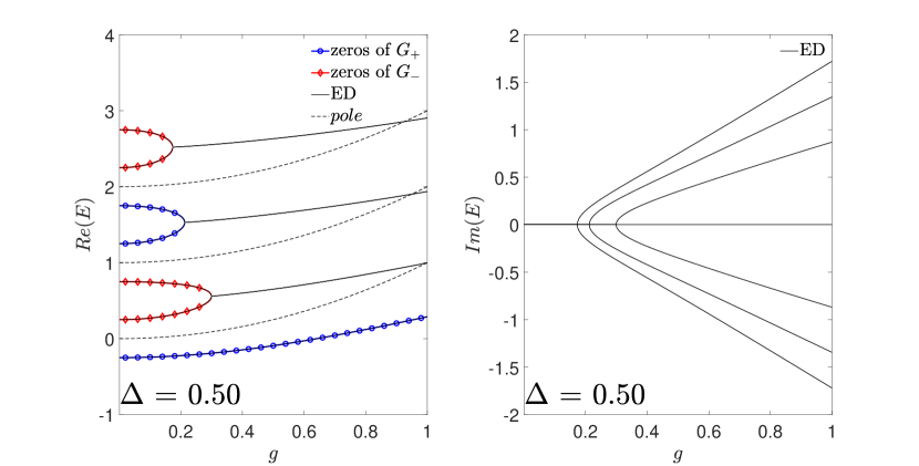
Figure 2: (colored online) Energy levels as a function of the coupling strength $g$ for $\Delta=0.50$. The black solid lines are eigenenergies obtained by the exact diagonalization (ED) method, and the dashed lines are $E_{n}^{(pole)}$. The blue lines with circles are zeros of $G_{+}$, and the red lines with diamonds are zeros of $G_{-}$.

The energy data by the numerical exact diagonalization agree well with the zeros of the $G$-function for real energy according to Fig. 2.

It is worth noting that the parity $\Pi_{1p}=\sigma_{x}\otimes e^{i\pi a^{\dagger}a}$ for the QRM still holds for the non-Hermitian QRM. $\pm$ in the G-function (10) just stand for the positive and negative parity, respectively, similar to the Hermitian case chen_exact_2012 . As discussed above, a pair of complex-conjugate levels are simultaneously determined by the zeros of either $G_{+}$ or $G_{-}$, thus possess the same parity.

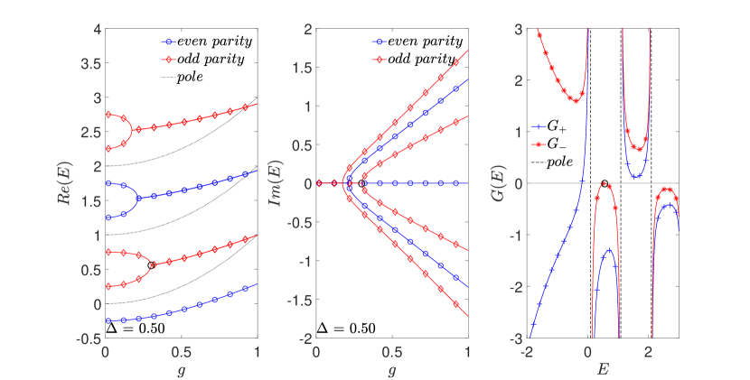
Figure 3: (colored online) Real energy levels as a function of the coupling strength $g$ for $\Delta=0.50$ (left panel), imaginary energy levels (middle panel), and $G$-function (right panel) corresponding to EP circled in black. The blue lines with circles are even $\Pi_{1p}$ parity levels, and the red lines with diamonds are odd $\Pi_{1p}$ parity levels. The dashed lines are $E_{n}^{(pole)}$. The blue lines with $+$ are $G_{+}$, and the red lines with $\ast$ are $G_{-}$.

An EP means that the $G$-function has only one zero between two adjacent poles. As shown in Fig. 3, the EP can be obtained when both the $G$-function and its first-order derivative with respect to energy are zero simultaneously.

$$\frac{\partial G_{\pm}}{\partial E}=\sum\left[\frac{\frac{\Delta}{2}f_{n}}{\left(n+g^{2}-E\right)^{2}}+\left(\frac{\frac{\Delta}{2}}{n+g^{2}-E}\mp 1\right)\frac{\partial f_{n}}{\partial E}\right]g^{n},$$ (12)

$$\frac{\partial f_{n}}{\partial E} = \frac{1}{2ng}\left(\frac{-\frac{\Delta^{2}}{4}}{\left(n-1+g^{2}-E\right)^{2}}-1\right)f_{n-1}+\frac{1}{n}\frac{\partial f_{n-2}}{\partial E}$$

$$+\frac{1}{2ng}\left(\frac{-\frac{\Delta^{2}}{4}}{n-1+g^{2}-E}+n-1-3g^{2}-E\right)\frac{\partial f_{n-1}}{\partial E}.$$

Now the eigenfunction can be expressed as

$$|\Psi\rangle=\begin{bmatrix}\sum i^{-n}\sqrt{n!}e_{n}D(-ig)|n\rangle\\ \pm\sum(-i)^{-n}\sqrt{n!}e_{n}D(ig)|n\rangle\end{bmatrix},$$ (13)

where $\pm$ correspond to eigenvalues $\pm 1$ of $\Pi_{1p}$. The $PT$ operator acts on $|\Psi\rangle$,

$$PT|\Psi\rangle = (\sigma_{x}\otimes\openone)T\begin{bmatrix}\sum i^{-n}\sqrt{n!}e_{n}D(-ig)|n\rangle\\ \pm\sum(-i)^{-n}\sqrt{n!}e_{n}D(ig)|n\rangle\end{bmatrix}$$ (14)

$$= \begin{bmatrix}\pm\sum i^{-n}\sqrt{n!}e_{n}^{\ast}D(-ig)|n\rangle\\ \sum(-i)^{-n}\sqrt{n!}e_{n}^{\ast}D(ig)|n\rangle\end{bmatrix}.$$

Before the EP, all $e_{n}$ are real, hence $PT|\Psi\rangle$ is simply $\pm|\Psi\rangle$, indicating the preservation of $\mathcal{PT}$ symmetry. After the EP, $\mathcal{PT}$ symmetry is broken, and $\{e_{n}^{\ast}\}$ for $E$ correspond to $\{e_{n}\}$ for $E^{\ast}$, leading to the $PT$ operator transforming $|\Psi\rangle$ into its conjugate counterpart.

The EPs can also be examined by calculating fidelity susceptibility

$$\chi=\frac{1-\langle L(\lambda)|R(\lambda+\epsilon)\rangle\langle L(\lambda+\epsilon)|R(\lambda)\rangle}{\epsilon^{2}},$$ (15)

where $|L\rangle$ and $|R\rangle$ are bra and ket of biorthogonal basis respectively tzeng_hunting_2021 . The limit of $Re(\chi(g))$ tends to negative infinity when $g$ approaches an EP, as illustrated in Fig. 4. Note that in the practical calculations, the truncation number of the summation in the G-function given by Eq. (10) cannot be really infinite, so the $Re(\chi(g))$ is only extremely negatively large.

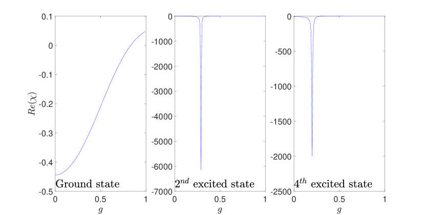
Figure 4: Fidelity susceptibility as a function of the coupling strength $g$ for the ground state(left panel), the $2^{nd}$ excited state(middle panel) and the $4^{th}$ excited state(right panel) at $\Delta=0.5$.

II.3 Generalized Rotating-wave Approximation

The conventional GRWA in the QRM involves a unitary transformation given by $D_{1p}=e^{g\sigma_{z}(a^{\dagger}-a)}$. In the non-Hermitian case that $g\rightarrow ig$, we introduce a similar transformation $D(ig)=e^{ig\sigma_{z}(a^{\dagger}-a)}$, and thus have.

$$H^{\prime} = D(ig)HD(-ig)=a^{\dagger}a+g^{2}-$$ (16)

$$\frac{\Delta}{2}\left[\sigma_{x}\cos 2g\left(a^{\dagger}-a\right)-\sigma_{y}\sin 2g\left(a^{\dagger}-a\right)\right].$$

Then a unitary transformation $S=\frac{1}{\sqrt{2}}\left(1-i\sigma_{y}\right)$ is applied,

$$\tilde{H} = SH^{\prime\dagger}=a^{\dagger}a+g^{2}$$ (17)

$$+\frac{\Delta}{2}\left[\sigma_{z}\cos 2g\left(a^{\dagger}-a\right)+\sigma_{y}\sin 2g\left(a^{\dagger}-a\right)\right].$$

Since

$$\langle m|D(i2g)|n\rangle = e^{-2g^{2}}\sqrt{\frac{m!}{n!}}(-2ig)^{n-m}L_{m}^{n-m}\left(-4g^{2}\right)$$

$$= (-1)^{n-m}\langle n|D(i2g)|m\rangle=D_{mn}\quad n\geq m,$$

where $L_{m}^{n-m}$ is Laguerre polynomial, and the domain of definition has been extended to $(-\infty,0)$, we have

$$\langle n|\sin 2g\left(a^{\dagger}-a\right)|n\rangle=\langle n|\cos 2g\left(a^{\dagger}-a\right)|n+1\rangle=0,$$

$$\langle n|\cos 2g\left(a^{\dagger}-a\right)|n\rangle=D_{nn},$$

$$\langle n|\sin 2g\left(a^{\dagger}-a\right)|n+1\rangle=-iD_{n,n+1}.$$ (18)

Neglecting the higher order terms, the Hamiltonian is reformed as

$$\tilde{H} = a^{\dagger}a+g^{2}+\frac{\Delta}{2}G(\hat{n})\sigma_{z}$$ (19)

$$+\frac{\Delta}{2}\left(\sigma_{+}-\sigma_{-}\right)\left[F(\hat{n})a-a^{\dagger}F^{\dagger}(\hat{n})\right],$$

where

$$G(\hat{n})|n\rangle=D_{nn}|n\rangle,\quad F(\hat{n})|n\rangle=-\frac{D_{n,n+1}}{\sqrt{n+1}}|n\rangle.$$

Eventually, we can have the following RWA form

$$H_{GRWA} = a^{\dagger}a+g^{2}+\frac{\Delta}{2}G(\hat{n})\sigma_{z}$$ (20)

$$+\frac{\Delta}{2}\left[F(\hat{n})a\sigma_{+}+\sigma_{-}a^{\dagger}F^{\dagger}(\hat{n})\right].$$

Now we can easily diagonalize the Hamiltonian based on the basis $\{|\uparrow,n\rangle,|\downarrow,n+1\rangle\}$

$$H_{n}^{GRWA}=\begin{bmatrix}n+g^{2}+\frac{\Delta}{2}D_{nn}&-\frac{\Delta}{2}D_{n,n+1}\\ \frac{\Delta}{2}D_{n,n+1}&n+1+g^{2}-\frac{\Delta}{2}D_{n+1,n+1}\end{bmatrix}.$$

It is straightforward to obtain the eigenvalues and corresponding eigenfunctions

$$E_{n}^{\pm} = n+g^{2}+\frac{1}{2}+\frac{\Delta e^{-2g^{2}}}{4}\left[L_{n}^{0}\left(-4g^{2}\right)-L_{n+1}^{0}\left(-4g^{2}\right)\right]$$ (21)

$$\pm\sqrt{\left[\frac{1}{2}-\frac{\Delta e^{-2g^{2}}\left(L_{n}^{0}\left(-4g^{2}\right)+L_{n+1}^{0}\left(-4g^{2}\right)\right)}{4}\right]^{2}-\frac{g^{2}\Delta^{2}e^{-4g^{2}}\left[L_{n}^{1}\left(-4g^{2}\right)\right]^{2}}{n+1}},$$

$$|\psi_{n}^{\pm}\rangle = \frac{1}{\sqrt{2}}\sqrt{1\pm\frac{\sqrt{x^{2}-y^{2}}}{x}}|\uparrow,n\rangle+\frac{ixy}{\sqrt{2}|xy|}\sqrt{1\mp\frac{\sqrt{x^{2}-y^{2}}}{x}}|\downarrow,n+1\rangle,\quad\text{in the $\mathcal{PT}$ regime};$$

$$|\psi_{n}^{\pm}\rangle = \frac{i}{\sqrt{2}}|\uparrow,n\rangle+\frac{1}{\sqrt{2}}\left(\pm i\frac{\sqrt{y^{2}-x^{2}}}{y}-\frac{x}{y}\right)|\downarrow,n+1\rangle,\quad\text{in the $\mathcal{PT}$-broken regime},$$ (22)

where

$$x = \frac{\Delta e^{-2g^{2}}\left(L_{n}^{0}\left(-4g^{2}\right)+L_{n+1}^{0}\left(-4g^{2}\right)\right)}{4}-\frac{1}{2},$$

$$y = \frac{g\Delta e^{-2g^{2}}L_{n}^{1}\left(-4g^{2}\right)}{\sqrt{n+1}}.$$ (23)

Specially, the energy of the ground-state is

$$E_{GS}=g^{2}-\frac{\Delta}{2}D_{00}=g^{2}-\frac{\Delta}{2}e^{-2g^{2}}.$$

$\mathcal{PT}$ symmetry is broken when $|x|\leq|y|$, the EP can be given analytically by the solution of $x=y$.

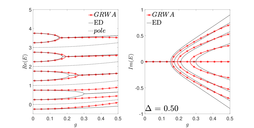
(a)

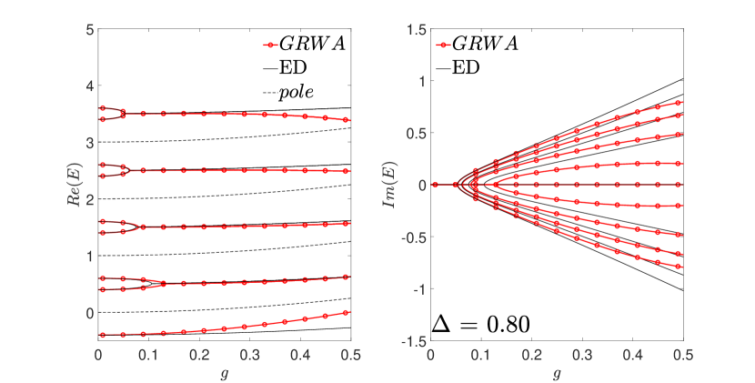
(b)

Figure 5: (colored online) Real energy (left panel) and imaginary energy (right panel) as a functions of $g$ for $\Delta=0.5$ (upper panel) and $\Delta=0.8$ (lower panel). The results obtained by both the numerical diagonal method (black lines) and GRWA (red lines) are collected for comparison.

As exhibited in Fig. 5, the GRWA performs quite well in the low detuning $\Delta$ regime and at the highly excited states. In the low panel of Fig. 5, the EPs under GRWA agree excellently with the exact solution for all cases except that at  the first two excited energy levels.

In the original space, the excited wave functions can be obtained by $|\Psi_{n}^{\pm}\rangle=D(ig)S^{\dagger}|\psi_{n}^{\pm}\rangle$

$$|\Psi_{n}^{\pm}\rangle = \frac{|\uparrow\rangle}{\sqrt{2}}D(-ig)\left(c_{n}^{\pm}|n\rangle+d_{n}^{\pm}|n+1\rangle\right)$$

$$+\frac{|\downarrow\rangle}{\sqrt{2}}D(ig)\left(d_{n}^{\pm}|n+1\rangle-c_{n}^{\pm}|n\rangle\right),$$

$$|\Psi_{GS}\rangle = \frac{1}{\sqrt{2}}\left[D(-ig)|\uparrow,0\rangle+D(ig)|\downarrow,0\rangle\right].$$ (24)

Note that $\Pi_{1p}|\Psi_{n}^{(\pm)}\rangle=(-1)^{n+1}|\Psi_{n}^{(\pm)}\rangle$ and $\Pi_{1p}|\Psi_{GS}\rangle=|\Psi_{GS}\rangle$, it follows that the parity $\Pi_{1p}$ is preserved for GRWA. In the $\mathcal{PT}$ regime, $PT|\Psi_{n}^{\pm}\rangle=(-1)^{n+1}|\Psi_{n}^{(\pm)}\rangle$, while in the $\mathcal{PT}$-broken regime, $PT|\Psi_{n}^{\pm}\rangle=|\Psi_{n}^{\mp}\rangle$. It is to note that the approximate GRWA methodology can preserve the essential feature of the non-Hermitian QRM, as the exact solution does.

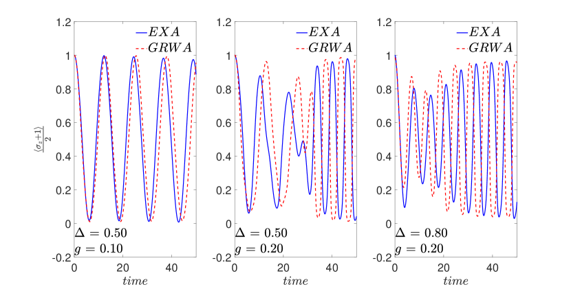
Figure 6: (colored online) Time evolution of the atomic population $\frac{\langle\sigma_{z}\rangle+1}{2}$ for $\Delta=0.50$, $g=0.10$ (left panel), $\Delta=0.50$, $g=0.20$ (middle panel), and $\Delta=0.80$, $g=0.20$ (right panel). The solid blue lines are numerically exact results, and the dashed red lines are GRWA results.

Upon analyzing the temporal evolution of the quantity $\frac{\langle\sigma_{z}\rangle+1}{2}$ with the initial state $|\Psi(0)\rangle=|\uparrow,0\rangle$ (Fig. 6), it is observed that the GRWA results can match basically the numerically exact ones.

III Non-Hermitian two-photon quantum Rabi model

Next, we turn to the non-Hermitian tpQRM described by the following Hamiltonian

$$H_{2pNH}=-\frac{\Delta}{2}\sigma_{x}+a^{\dagger}a+ig\left(a^{2}+(a^{\dagger})^{2}\right)\sigma_{z},$$ (25)

which is a natural extension of the non-Hermitian QRM.

The parity operator $P=\sigma_{x}\otimes\openone$ and the time-reversal operator $T$ defined before still satisfy

$$PTH_{2pNH}TP = P\left(a^{\dagger}a-ig\left(a^{2}+(a^{\dagger})^{2}\right)\sigma_{z}-\frac{\Delta}{2}\sigma_{x}\right)P$$ (26)

$$= a^{\dagger}a+ig\left(a^{2}+(a^{\dagger})^{2}\right)\sigma_{z}-\frac{\Delta}{2}\sigma_{x}=H.$$

Therefore, this Hamiltonian is also $\mathcal{PT}$-symmetric.

III.1 Solutions within Bogoliubov transformation

The $G$-function for non-Hermitian tpQRM can be derived in a similar way as for tpQRM duan_two-photon_2016 . Analogously, a similar transformation

$$S(ir)=e^{i\frac{r}{2}\left((a^{\dagger})^{2}-a^{2}\right)}$$

where

$$r=\frac{1}{2}\cos^{-1}{\frac{1}{\sqrt{1+4g^{2}}}}.$$ (27)

is introduced, thus we have

$$S(ir)aS(-ir)=a\cos{r}-ia^{\dagger}\sin{r},$$

$$S(ir)a^{\dagger}S(-ir)=a^{\dagger}\cos{r}-ia\sin{r},$$

$$S(ir)S(-ir)=1,\quad S(ir)^{\dagger}S(ir)=S(2ir)\neq 1.$$ (28)

Hamiltonian (25) is then reformed by two opposite transformation

$$H_{+}^{2p}=S(ir)H_{2pNH}S(-ir)=$$

$$\begin{bmatrix}\sqrt{1+4g^{2}}\left(a^{\dagger}a+\frac{1}{2}\right)-\frac{1}{2}&-\frac{\Delta}{2}\\ -\frac{\Delta}{2}&\frac{\left(1-4g^{2}\right)\left(a^{\dagger}a+\frac{1}{2}\right)-2ig\left(a^{2}+(a^{\dagger})^{2}\right)}{\sqrt{1+4g^{2}}}-\frac{1}{2}\end{bmatrix},$$

$$H_{-}^{2p}=S(-ir)H_{2pNH}S(ir)=$$

$$\begin{bmatrix}\frac{\left(1-4g^{2}\right)\left(a^{\dagger}a+\frac{1}{2}\right)+2ig\left(a^{2}+(a^{\dagger})^{2}\right)}{\sqrt{1+4g^{2}}}-\frac{1}{2}&-\frac{\Delta}{2}\\ -\frac{\Delta}{2}&\sqrt{1+4g^{2}}\left(a^{\dagger}a+\frac{1}{2}\right)-\frac{1}{2}\end{bmatrix}.$$

Next, we define a set of ladder operators which satisfy Lie algebra,

$$K_{0}=\frac{1}{2}\left(a^{\dagger}a+\frac{1}{2}\right),\quad K_{+}=\frac{1}{2}\left(a^{\dagger}\right)^{2},\quad K_{-}=\frac{1}{2}a^{2},$$ (30)

where

$$\left[K_{0},K_{\pm}\right]=\pm K_{\pm},\left[K_{+},K_{-}\right]=-2K_{0}.$$ (31)

The Hilbert space $\mathcal{H}$ generated by $a^{\dagger}$ acting on the photon vacuum state $|0\rangle$, decays into two subspaces characterized by the so-called Bargmann index $q$: $K_{0}|q,0\rangle=q|q,0\rangle$. For the even photonic subspace $\mathcal{H}_{\frac{1}{4}}=\left\{\left(a^{\dagger}\right)^{n}\left|0\right\rangle,n=0,2,4......\right\}$, $q=\frac{1}{4}$ and for the odd photonic subspace $\mathcal{H}_{\frac{3}{4}}=\left\{\left(a^{\dagger}\right)^{n}\left|0\right\rangle,n=1,3,5......\right\}$, $q=\frac{3}{4}$.

$$\left|q,n\right\rangle = \left|2\left(q+n-\frac{1}{4}\right)\right\rangle=\frac{\left(a^{\dagger}\right)^{2\left(q+n-\frac{1}{4}\right)}}{\sqrt{\left[2\left(q+n-\frac{1}{4}\right)\right]!}}\left|0\right\rangle,$$

$$K_{0}\left|q,n\right\rangle = (q+n)\left|q,n\right\rangle,$$

$$K_{+}\left|q,n\right\rangle = \sqrt{\left(n+q+\frac{1}{4}\right)\left(n+q+\frac{3}{4}\right)}\left|q,n+1\right\rangle,$$

$$K_{-}\left|q,n\right\rangle = \sqrt{\left(n+q-\frac{1}{4}\right)\left(n+q-\frac{3}{4}\right)}\left|q,n-1\right\rangle.$$

In term of $K_{0},K_{\pm}$, the Hamiltonian $H_{+}^{2p}$ becomes

$$H_{+}^{2p}=\begin{bmatrix}2K_{0}\sqrt{1+4g^{2}}-\frac{1}{2}&-\frac{\Delta}{2}\\ -\frac{\Delta}{2}&\frac{2K_{0}(1-4g^{2})-4ig(K_{+}+K_{-})}{\sqrt{1+4g^{2}}}-\frac{1}{2}\end{bmatrix}.$$ (32)

Now, we propose the general expansion for the eigenfunction of $H_{+}^{2p}$ as

$$\left|+^{(q)}\right\rangle=\begin{bmatrix}\sum\sqrt{\left[2\left(n+q-\frac{1}{4}\right)\right]!}i^{n}e_{n}^{(q)}\left|q,n\right\rangle\\ \sum\sqrt{\left[2\left(n+q-\frac{1}{4}\right)\right]!}i^{n}f_{n}^{(q)}\left|q,n\right\rangle\end{bmatrix},$$ (33)

where $e_{n}^{(q)}$ and $f_{n}^{(q)}$ are the expansion coefficients. By the Schrödinger equation $H_{+}\left|\psi^{(q)}\right\rangle=E\left|\psi^{(q)}\right\rangle$ and projecting onto $|q,n\rangle$, a recursive relation of $e_{n}^{(q)}$ and $f_{n}^{(q)}$ is derived as

$$e_{n}^{(q)}=\frac{\frac{\Delta}{2}f_{n}^{(q)}}{2(n+q)\sqrt{1+4g^{2}}-\frac{1}{2}-E},$$ (34a)

$$f_{n+1}^{(q)} = \frac{\left[2(n+q)(1-4g^{2})-\sqrt{1+4g^{2}}\left(\frac{1}{2}+E\right)\right]f_{n}^{(q)}}{4g\left(n+q+\frac{1}{4}\right)\left(n+q+\frac{3}{4}\right)}$$

$$+\frac{4gf_{n-1}^{(q)}-\frac{\Delta}{2}\sqrt{1+4g^{2}}e_{n}^{(q)}}{4g\left(n+q+\frac{1}{4}\right)\left(n+q+\frac{3}{4}\right)}.$$

Similarly, the general expansion for the eigenfunction of $H_{-}$ can be expressed as

$$\left|-^{(q)}\right\rangle=\begin{bmatrix}\sum\sqrt{\left[2\left(n+q-\frac{1}{4}\right)\right]!}(-i)^{n}f_{n}^{(q)}\left|q,n\right\rangle\\ \sum\sqrt{\left[2\left(n+q-\frac{1}{4}\right)\right]!}(-i)^{n}e_{n}^{(q)}\left|q,n\right\rangle\end{bmatrix}.$$ (35)

Transforming back to the original Hamiltonian, we have

$$|\Psi^{(q)}\rangle_{+}=S(-ir)|+^{(q)}\rangle,\quad|\Psi^{(q)}\rangle_{-}=S(ir)|-^{(q)}\rangle.$$ (36)

These eigenfunctions should describe the same eigenstate, i.e. $\left|\Psi^{(q)}\right\rangle_{+}\propto\left|\Psi^{(q)}\right\rangle_{-}$. Projecting onto the photon vacuum state $\left|0\right\rangle$, we have

$$\langle 0|S(ir)|q,n\rangle\propto\frac{\sqrt{\left[2\left(n+q-\frac{1}{4}\right)\right]!}}{n!}\left(\frac{i\tan{r}}{2}\right)^{n}$$ (37)

$$\begin{bmatrix}\sum e_{n}^{(q)}\frac{\left[2\left(n+q-\frac{1}{4}\right)\right]!}{n!}\left(\frac{\tan{r}}{2}\right)^{n}\\ \sum f_{n}^{(q)}\frac{\left[2\left(n+q-\frac{1}{4}\right)\right]!}{n!}\left(\frac{\tan{r}}{2}\right)^{n}\end{bmatrix}\propto\begin{bmatrix}\sum f_{n}^{(q)}\frac{\left[2\left(n+q-\frac{1}{4}\right)\right]!}{n!}\left(\frac{\tan{r}}{2}\right)^{n}\\ \sum e_{n}^{(q)}\frac{\left[2\left(n+q-\frac{1}{4}\right)\right]!}{n!}\left(\frac{\tan{r}}{2}\right)^{n}\end{bmatrix}.$$

The $G$-function is finally formulated as

$$G_{\pm}^{(q)}=\sum\left(e_{n}^{(q)}\mp f_{n}^{(q)}\right)\frac{\left[2\left(n+q-\frac{1}{4}\right)\right]!}{n!}\left(\frac{\tan{r}}{2}\right)^{n},$$

all $e_{n}^{(q)}$ and $f_{n}^{(q)}$ can be determined by recursive relation Eq. (34) and $e_{0}^{(q)}=1$. Zeros of $G_{\pm}^{(q)}$ will give all eigenenergies of the non-Hermitian tpQRM. According to Eq. (34), the nth pole for $G_{\pm}^{(q)}$ is

$$E_{n}^{(q,pole)}=2(n+q)\sqrt{1+4g^{2}}-\frac{1}{2},$$ (38)

one immediately finds that the spectral collapse in duan_two-photon_2016 does not happen in the corresponding non-Hermitian case, which can be also exhibited in Fig. 7.

Figure 7: Real energy levels (left panel) and imaginary energy (right panel) as functions of the coupling strength $g$ for $\Delta=0.50$ and $q=\frac{1}{4}$. The solid lines are eigenenergies obtained by the numerical diagonal method, and the dashed lines are $E_{n}^{(pole)}$.

The zeros for the $G$-function vanish at the high-$E$ regime as detailed in Fig. 8, indicating the presence of complex eigenenergies. Since only $E$ is complex in parameters of the recursive relation Eq. (34), $G_{\pm}^{(q)}(E^{\ast})=G_{\pm}^{\ast(q)}(E)$. Therefore, if $E$ is a solution, both $E$ and $E^{\ast}$ are the solutions of either $G_{+}^{(q)}=0$ or $G_{-}^{(q)}=0$.

.

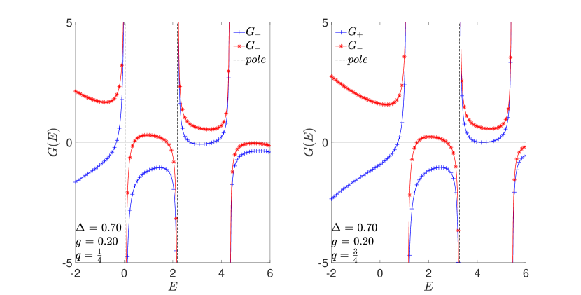
Figure 8: (colored online) G-curves for $\Delta=0.70$, $g=0.20$ in the real E regime, $q=\frac{1}{4}$ (left panel) and $q=\frac{3}{4}$ (right panel). The blue lines with $+$ marks and the red lines with $\ast$ marks are $G_{+}$ and $G_{-}$ curves, respectively. The black dashed lines are $E_{n}^{(q,pole)}$

III.2 Exceptional Points and Symmetry

The EPs can be presented with the emergence of complex eigenenergies, while the tpQRM parity $\Pi_{2p}=\sigma_{x}\otimes e^{i\frac{\pi a^{\dagger}a}{2}}$ remains unaltered. Similar to the non-Hermitian QRM, a pair of conjugate levels of non-Hermitian tpQRM also share the same parity with $G_{\pm}^{(q)}(E^{\ast})=G_{\pm}^{(q)\ast}(E)$.

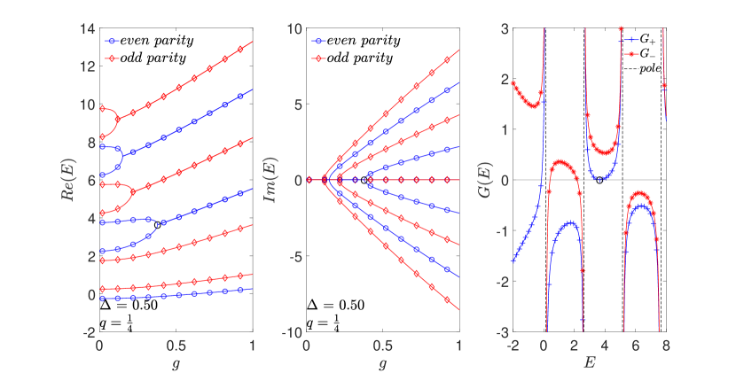
Figure 9: (colored online) Real energy levels as a function of the coupling strength $g$ for $\Delta=0.50$ (left panel), imaginary energy levels (middle panel), and the $G$-function (right panel) corresponding to the EP circled in black. The blue lines with circles are even $\Pi_{2p}$ parity levels, and the red lines with diamonds are odd $\Pi_{2p}$ parity levels. The blue lines with $+$ are $G_{+}$ and the red lines with $*$ are $G_{-}$.

An EP means that the $G$-function has only one zero between two adjacent poles. As can be seen in Fig. 9, taking the derivative with respect to energy, the EP can still be obtained when both the $G$-function and its derivative with respect to energy are zero.

Therefore, the eigenfunction can be expressed as

$$\left|\Psi^{(q)}\right\rangle=\begin{bmatrix}\sum\sqrt{\left[2\left(n+q-\frac{1}{4}\right)\right]!}i^{n}e_{n}^{(q)}S(-ir)\left|q,n\right\rangle\\ \pm\sum\sqrt{\left[2\left(n+q-\frac{1}{4}\right)\right]!}(-i)^{n}e_{n}^{(q)}S(ir)\left|q,n\right\rangle\end{bmatrix}$$

where $\pm$ stands for the even and odd tpQRM parity.

Then the $PT$ operator acts on the wave function Eq. (III.2),

$$PT\left|\Psi^{(q)}\right\rangle$$ (39)

$$= \sigma_{x}\otimes T\begin{bmatrix}\sum\sqrt{\left[2\left(n+q-\frac{1}{4}\right)\right]!}i^{n}e_{n}^{(q)}S(-ir)\left|q,n\right\rangle\\ \pm\sum\sqrt{\left[2\left(n+q-\frac{1}{4}\right)\right]!}(-i)^{n}e_{n}^{(q)}S(ir)\left|q,n\right\rangle\end{bmatrix}$$

$$= \begin{bmatrix}\pm\sum\sqrt{\left[2\left(n+q-\frac{1}{4}\right)\right]!}i^{n}e_{n}^{(q)\ast}S(-ir)\left|q,n\right\rangle\\ \sum\sqrt{\left[2\left(n+q-\frac{1}{4}\right)\right]!}(-i)^{n}e_{n}^{(q)\ast}S(ir)\left|q,n\right\rangle\end{bmatrix}.$$

In the $\mathcal{PT}$ regime, real energy results in real $e_{n}^{(q)}$ and $f_{n}^{(q)}$, leading to $PT|\Psi^{(q)}\rangle=\pm|\Psi^{(q)}\rangle$. Meanwhile, in the $\mathcal{PT}$-broken regime, $\{e_{n}^{(q)\ast}\}$ are identical to $\{e_{n}^{(q)}\}$ corresponding to $E^{\ast}$, analogous to the non-Hermitian QRM. In conclusion, we have proved that the $PT$ operator transforms the eigenstate to its conjugate counterpart in the $\mathcal{PT}$-broken regime.

The $\mathcal{PT}$ symmetry can be broken with the emergence of complex eigenenergies at large coupling strength (EP is the critical value), while the original parity $\Pi_{2p}=\sigma_{x}\otimes e^{i\frac{\pi a^{\dagger}a}{2}}$ of the tpQRM remains unaltered of the same level in the whole coupling regime.

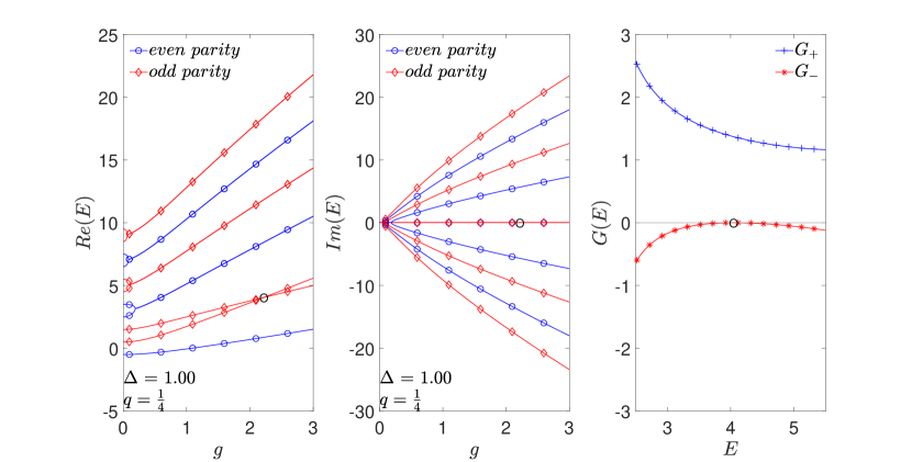
Figure 10: (colored online) Real energy levels as a function of coupling strength $g$ for $\Delta=1.00$ (left panel), imaginary energy levels (middle panel), and the $G$-function (right panel) corresponding to the EP circled in black. The blue lines with circle marks are even $\Pi_{2p}$ parity levels, and the red lines with diamond marks are odd $\Pi_{2p}$ parity levels. The blue lines with $+$ marks are $G_{+}$ and the red lines with $\ast$ marks are $G_{-}$.

III.3 Exceptional Point for Real Levels

Precisely at the resonance $\Delta=1$, it is noteworthy that an EP emerges at the lowest two excited states with real energies, as displayed in Fig. 10. The $G$-function corresponding to the EP exhibits only one zero, indicating that eigenfunctions for the intersecting real levels are identical at the EP.

Slightly deviation from $\Delta=1$, say $\Delta=0.99$ and $\Delta=1.01,$ the EP of real levels disappears, which is clearly shown in Fig. 11. It is surprising that $\Delta=1$ serves as the only condition for the existence of the exotic real-level EP.

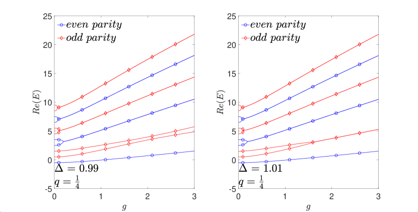
Figure 11: (colored online) Real energy levels as a function of the coupling strength $g$ for $\Delta=0.99$ (left panel), and $\Delta=1.01$ (right panel). The blue lines with circles are even $\Pi_{2p}$ parity levels, and the red lines with diamonds are odd $\Pi_{2p}$ parity levels.

By calculating the fidelity susceptibility $\chi$, it is observed that the real part of $\chi(g)$ tends to negative infinity as $g$ approaches EPs, including the real-level EP, as shown in Fig. 12. This suggests that the real-level crossing point is truly an EP, but may be a new kind of EPs.

Figure 12: The fidelity susceptibility as a function of the coupling strength $g$ for the $1^{st}$ excited state (left panel), the $3^{rd}$ excited state (middle panel) and the $5^{th}$ excited state (right panel) at $\Delta=1.0$.

IV Summary

In this work, we have compactly derived the $G$-function for the non-Hermitian QRM and tpQRM using the Bogoliuvbov operators approach, whose zeros determine the energy spectrum. Specifically, in the $\mathcal{PT}$ regime, the $G$-function is defined in real variable space. Therefore, the EPs can be detected when both the $G$-function and its derivative with respect to $E$ are zero. Through the $G$-function, we have confirmed the complex-conjugate spectra of non-Hermitian systems with $\mathcal{PT}$ symmetry, and in the $\mathcal{PT}$-broken regime, the $PT$ operator transforms one eigenstate to its conjugate counterpart. Many EPs are located within the two nearest-neighboring energy levels, thus the number of EPs is infinite. With higher energy levels, the EP shrinks to the smaller coupling strength. The conventional GRWA can preserve the relevant $\mathcal{PT}$ properties. The fidelity susceptibility goes to negative infinity around the EPs, consistent with the recent observation in other non-Hermitian systems.

Remarkably, the lowest two excited levels with real energies in the non-Hermitian tpQRM at $\Delta=1$ exhibit a novel EP. This real-level EP may be of fundamental importance in non-Hermitian systems. The hidden symmetry implied by the true crossing of real levels within the same parity and the same Bargmann index in the tpQRM is yet to be identified. Further study is needed to clarify this issue.

- [1] Joshua Feinberg and A. Zee. Non-Hermitian localization and delocalization. Physical Review E, 59(6):6433–6443, June 1999.
- [2] Jie Ren, Peter Hänggi, and Baowen Li. Berry-Phase-Induced Heat Pumping and Its Impact on the Fluctuation Theorem. Physical Review Letters, 104(17):170601, April 2010.
- [3] Stefano Longhi. Non-Hermitian quantum rings. Physical Review A, 88(6):062112, December 2013.
- [4] Tony E. Lee and Ching-Kit Chan. Heralded Magnetism in Non-Hermitian Atomic Systems. Physical Review X, 4(4):041001, October 2014.
- [5] Xing Gao and Walter Thiel. Non-Hermitian surface hopping. Physical Review E, 95(1):013308, January 2017.
- [6] Kai Li and Yong Xu. Non-Hermitian Absorption Spectroscopy. Physical Review Letters, 129(9):093001, August 2022.
- [7] Dorje C Brody. Biorthogonal quantum mechanics. Journal of Physics A: Mathematical and Theoretical, 47(3):035305, January 2014.
- [8] Andreas Fring and Thomas Frith. Exact analytical solutions for time-dependent Hermitian Hamiltonian systems from static unobservable non-Hermitian Hamiltonians. Physical Review A, 95(1):010102, January 2017.
- [9] Yuto Ashida, Zongping Gong, and Masahito Ueda. Non-Hermitian physics. Advances in Physics, 69(3):249–435, July 2020.
- [10] Yu-Chin Tzeng, Chia-Yi Ju, Guang-Yin Chen, and Wen-Min Huang. Hunting for the non-Hermitian exceptional points with fidelity susceptibility. Physical Review Research, 3(1):013015, January 2021.
- [11] Elisabet Edvardsson and Eddy Ardonne. Sensitivity of non-Hermitian systems. Physical Review B, 106(11):115107, September 2022.
- [12] Carl M. Bender and Stefan Boettcher. Real Spectra in Non-Hermitian Hamiltonians Having P T Symmetry. Physical Review Letters, 80(24):5243–5246, June 1998.
- [13] Ali Mostafazadeh. Pseudo-Hermiticity versus PT symmetry: The necessary condition for the reality of the spectrum of a non-Hermitian Hamiltonian. Journal of Mathematical Physics, 43(1):205–214, January 2002.
- [14] Ali Mostafazadeh. Pseudo-Hermiticity versus PT-symmetry. II. A complete characterization of non-Hermitian Hamiltonians with a real spectrum. Journal of Mathematical Physics, 43(5):2814–2816, May 2002.
- [15] Carl M Bender. PT -symmetric quantum theory. Journal of Physics: Conference Series, 631:012002, July 2015.
- [16] Christian E. Rüter, Konstantinos G. Makris, Ramy El-Ganainy, Demetrios N. Christodoulides, Mordechai Segev, and Detlef Kip. Observation of parity–time symmetry in optics. Nature Physics, 6(3):192–195, March 2010.
- [17] Liang Feng, Zi Jing Wong, Ren-Min Ma, Yuan Wang, and Xiang Zhang. Single-mode laser by parity-time symmetry breaking. Science, 346(6212):972–975, November 2014.
- [18] Vladimir V. Konotop, Jianke Yang, and Dmitry A. Zezyulin. Nonlinear waves in PT-symmetric systems. Reviews of Modern Physics, 88(3):035002, July 2016.
- [19] Ramy El-Ganainy, Konstantinos G. Makris, Mercedeh Khajavikhan, Ziad H. Musslimani, Stefan Rotter, and Demetrios N. Christodoulides. Non-Hermitian physics and PT symmetry. Nature Physics, 14(1):11–19, January 2018.
- [20] Wei-Chen Wang, Yan-Li Zhou, Hui-Lai Zhang, Jie Zhang, Man-Chao Zhang, Yi Xie, Chun-Wang Wu, Ting Chen, Bao-Quan Ou, Wei Wu, Hui Jing, and Ping-Xing Chen. Observation of PT-symmetric quantum coherence in a single-ion system. Physical Review A, 103(2):L020201, February 2021.
- [21] Mohammad-Ali Miri and Andrea Alù. Exceptional points in optics and photonics. Science, 363(6422):eaar7709, January 2019.
- [22] Ş. K. Özdemir, S. Rotter, F. Nori, and L. Yang. Parity–time symmetry and exceptional points in photonics. Nature Materials, 18(8):783–798, August 2019.
- [23] Aodong Li, Heng Wei, Michele Cotrufo, Weijin Chen, Sander Mann, Xiang Ni, Bingcong Xu, Jianfeng Chen, Jian Wang, Shanhui Fan, Cheng-Wei Qiu, Andrea Alù, and Lin Chen. Exceptional points and non-Hermitian photonics at the nanoscale. Nature Nanotechnology, June 2023.
- [24] I. I. Rabi. On the Process of Space Quantization. Physical Review, 49(4):324–328, February 1936.
- [25] Marlan O. Scully and M. Suhail Zubairy. Quantum Optics. Cambridge University Press, 1997.
- [26] D. Leibfried, R. Blatt, C. Monroe, and D. Wineland. Quantum dynamics of single trapped ions. Reviews of Modern Physics, 75(1):281–324, March 2003.
- [27] Dirk Englund, Andrei Faraon, Ilya Fushman, Nick Stoltz, Pierre Petroff, and Jelena Vučković. Controlling cavity reflectivity with a single quantum dot. Nature, 450(7171):857–861, December 2007.
- [28] K. Hennessy, A. Badolato, M. Winger, D. Gerace, M. Atatüre, S. Gulde, S. Fält, E. L. Hu, and A. Imamoğlu. Quantum nature of a strongly coupled single quantum dot–cavity system. Nature, 445(7130):896–899, February 2007.
- [29] T. Niemczyk, F. Deppe, H. Huebl, E. P. Menzel, F. Hocke, M. J. Schwarz, J. J. Garcia-Ripoll, D. Zueco, T. Hümmer, E. Solano, A. Marx, and R. Gross. Circuit quantum electrodynamics in the ultrastrong-coupling regime. Nature Physics, 6(10):772–776, October 2010.
- [30] Daniel Braak, Qing-Hu Chen, Murray T Batchelor, and Enrique Solano. Semi-classical and quantum Rabi models: in celebration of 80 years. Journal of Physics A: Mathematical and Theoretical, 49(30):300301, July 2016.
- [31] P. Forn-Díaz, J. J. García-Ripoll, B. Peropadre, J.-L. Orgiazzi, M. A. Yurtalan, R. Belyansky, C. M. Wilson, and A. Lupascu. Ultrastrong coupling of a single artificial atom to an electromagnetic continuum in the nonperturbative regime. Nature Physics, 13(1):39–43, January 2017.
- [32] P. Forn-Díaz, L. Lamata, E. Rico, J. Kono, and E. Solano. Ultrastrong coupling regimes of light-matter interaction. Reviews of Modern Physics, 91(2):025005, June 2019.
- [33] P. Bertet, S. Osnaghi, P. Milman, A. Auffeves, P. Maioli, M. Brune, J. M. Raimond, and S. Haroche. Generating and Probing a Two-Photon Fock State with a Single Atom in a Cavity. Physical Review Letters, 88(14):143601, March 2002.
- [34] S. Stufler, P. Machnikowski, P. Ester, M. Bichler, V. M. Axt, T. Kuhn, and A. Zrenner. Two-photon Rabi oscillations in a single quantum dot. Physical Review B, 73(12):125304, March 2006.
- [35] Elena Del Valle, Stefano Zippilli, Fabrice P. Laussy, Alejandro Gonzalez-Tudela, Giovanna Morigi, and Carlos Tejedor. Two-photon lasing by a single quantum dot in a high- Q microcavity. Physical Review B, 81(3):035302, January 2010.
- [36] S. Felicetti, J. S. Pedernales, I. L. Egusquiza, G. Romero, L. Lamata, D. Braak, and E. Solano. Spectral collapse via two-phonon interactions in trapped ions. Physical Review A, 92(3):033817, September 2015.
- [37] D. Braak. Integrability of the Rabi Model. Physical Review Letters, 107(10):100401, August 2011.
- [38] Qing-Hu Chen, Chen Wang, Shu He, Tao Liu, and Ke-Lin Wang. Exact solvability of the quantum Rabi model using Bogoliubov operators. Physical Review A, 86(2):023822, August 2012.
- [39] Liwei Duan, Shu He, Daniel Braak, and Qing-Hu Chen. Solution of the two-mode quantum Rabi model using extended squeezed states. EPL (Europhysics Letters), 112(3):34003, November 2015.
- [40] Liwei Duan, You-Fei Xie, Daniel Braak, and Qing-Hu Chen. Two-photon Rabi model: analytic solutions and spectral collapse. Journal of Physics A: Mathematical and Theoretical, 49(46):464002, November 2016.
- [41] You-Fei Xie, Liwei Duan, and Qing-Hu Chen. Quantum Rabi–Stark model: solutions and exotic energy spectra. Journal of Physics A: Mathematical and Theoretical, 52(24):245304, June 2019.
- [42] Jiong Li and Qing-Hu Chen. Two-photon Rabi–Stark model. Journal of Physics A: Mathematical and Theoretical, 53(31):315301, August 2020.
- [43] You-Fei Xie and Qing-Hu Chen. Double degeneracy associated with hidden symmetries in the asymmetric two-photon Rabi model. Physical Review Research, 3(3):033057, July 2021.
- [44] Tony E. Lee and Yogesh N. Joglekar. PT -symmetric Rabi model: Perturbation theory. Physical Review A, 92(4):042103, October 2015.
- [45] Qiongtao Xie, Shiguang Rong, and Xiaoliang Liu. Exceptional points in a time-periodic parity-time-symmetric Rabi model. Physical Review A, 98(5):052122, November 2018.
- [46] Xilin Lu, Hui Li, Jia-Kai Shi, Li-Bao Fan, Vladimir Mangazeev, Zi-Min Li, and Murray T. Batchelor. PT -symmetric quantum Rabi model. Physical Review A, 108(5):053712, November 2023.
- [47] E. K. Irish. Generalized Rotating-Wave Approximation for Arbitrarily Large Coupling. Physical Review Letters, 99(17):173601, October 2007.