HyperMagNet: A Magnetic Laplacian based Hypergraph Neural Network

Abstract.

In data science, hypergraphs are natural models for data exhibiting multi-way relations, whereas graphs only capture pairwise. Nonetheless, many proposed hypergraph neural networks effectively reduce hypergraphs to undirected graphs via symmetrized matrix representations, potentially losing important information. We propose an alternative approach to hypergraph neural networks in which the hypergraph is represented as a non-reversible Markov chain. We use this Markov chain to construct a complex Hermitian Laplacian matrix — the magnetic Laplacian — which serves as the input to our proposed hypergraph neural network. We study HyperMagNet for the task of node classification, and demonstrate its effectiveness over graph-reduction based hypergraph neural networks.

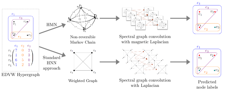
Figure 1. HyperMagNet (HMN) uses a non-reversible Markov chain to build a hypergraph Laplacian which avoids Laplacians associated with the star graph or clique expansion.

1. Introduction

A fundamental limitation of graphs in data science and machine learning is the relationships that a graph models are necessarily pairwise: edges connect exactly two vertices in a graph. For example, a graph edge may indicate two documents within a corpus share common vocabulary, two pixels in an image belong to the same neighborhood, or two diseases result from mutations in the same gene. However, these relationships are emphatically not only pairwise, but involve interactions between groups of documents, pixels, and diseases. Across these and other domains, modeling multi-way relationships with a graph therefore loses key information in the data. Hypergraphs, which allow more than two vertices to be connected by an edge, faithfully capture the multi-way relationships graphs cannot capture (aksoy2020hypernetwork, ) (bretto2013hypergraph, ) (feng2019hypergraph, ). Data that is set-valued, tabular, or bipartite is best modeled with a hypergraph.

Despite being a more expressive and general model than a graph, analyzing hypergraph data presents challenges. In machine learning tasks, one must first choose a representation of the hypergraph to be processed by a chosen algorithm. For example, convolutional neural networks use a Hermitian matrix representation of the hypergraph in order to learn optimal node embeddings via matrix multiplication with learnable weight matrices. However, classic matrix representations of graphs such as the adjacency matrix or the graph Laplacian have no direct analogues for hypergraphs. To overcome this challenge, representations of a hypergraph via a random walk have proved convenient. Zhou et al. (zhou2006learning, ) demonstrated this, defining a clustering algorithm based on a reversible random walk and the eigenvectors of an associated hypergraph Laplacian. Building on this representation and inspired by the success of graph convolutional neural networks (GCN), the seminal hypergraph neural network HGNN (feng2019hypergraph, ) uses Zhou’s hypergraph Laplacian in a traditional GCN defined by Kipf and Welling (kipf2016semi, ) for classification tasks in visual object recognition and citation network classification.

Unfortunately, it is known (agarwal2006higher, ) that Zhou’s hypergraph Laplacian indeed reduces to a graph Laplacian on the star graph corresponding to a hypergraph, and other Laplacians reduce to those of the clique graph. In this sense, these Laplacians and the aforementioned hypergraph neural network HGNN reduce a hypergraph to a graph. The reason this information loss occurs is because these matrices are based on reversible random walks, which always reduce to a random walk on an undirected graph (chitra2019random, ). Thus, a more faithful approach is to define Laplacians based on non-reversible random walks. As shown by Chitra and Raphael (chitra2019random, ), hypergraph random walks which utilize edge-dependent vertex weights (EDVW), in which transition probabilities are guided by vertex-hyperedge specific weightings, may be non-reversible. These weights, which allow vertices to have varying importance across the hyperedges to which they belong, often naturally present in data or may also be derived from structural properties of unweighted hypergraph data.

In this work, we build and study a hypergraph neural network that doesn’t rely on a star graph or clique expansion reduction Laplacian. Rather, our proposed HyperMagNet begins with a non-reversible hypergraph random walk that is more faithful in capturing nuances within hypergraph data, which are reflected as asymmetries in transition probabilities. However, the transition probability matrix representing this random walk is not Hermitian which complicates their use within traditional convolutional neural networks. Instead of overcoming this by only symmetrizing the transition matrix (thereby converting to a reversible, graph-based random walk), we instead encode it as a complex-valued, Hermitian-but-asymmetric matrix called the magnetic Laplacian. This Laplacian has been successfully applied in the graph learning community to directed graphs (fanuel2017magnetic, ) (zhang2021magnet, ) (shubin1994discrete, ). Studying its application in a hypergraph setting, we explain how to learn parameters of the magnetic Laplacian from hypergraph data, and build a hypergraph neural network around it. Finally, we investigate the efficacy of this approach, in comparison to HGNN and related graph-reduction methods for the task of node classification. On varied data, we find that HyperMagNet outperforms competing graph-based methods, sometimes modestly and sometimes significantly, and include experiments to test whether this increase in performance is due to the utilization of edge-dependent vertex weights, the magnetic Laplacian, or both. Although slightly more expensive to run, HyperMagNet is worth using due to its increase in performance over graph-reduction based models, as shown across several data modalities.

The paper is structured as follows: in Section 2, we provide background on hypergraphs, hypergraph random walks, and the magnetic Laplacian. In Section 3 we show how the magnetic Laplacian is an appropriate hypergraph Laplacian for the EDVW random walk and include comparisons with traditional hypergraph random walks and Laplacians based on clique graphs. We also introduce the neural network architecture of HyperMagNet in this section. Section 4 contains related work on hypergraph neural networks with and without EDVW. In Section 5 are experimental results in the tasks of node classification on a variety of hypergraph structured data sets, where performance is compared against a variety of machine learning models based on traditional graph-based representations.

2. Background

2.1. Hypergraphs and Random Walks

A hypergraph $H=(V,E)$ is a set of vertices $V=\{v_{1},\ldots,v_{n}\}$ and hyperedges $E=(e_{1},\ldots,e_{m})$ where each $e_{i}\subset V$ for $i=1,2,\ldots,m$. The key difference between a graph and a hypergraph is that the cardinality of the hyperedges is allowed to be greater than two. A graph is a special case of a hypergraph where the cardinality of the hyperedges are all equal to two, $|e_{i}|=2,$ for $i=1,2,\ldots,m$. The vertex-hyperedge relationship is typically stored in its incidence matrix indicating which vertices are contained in which hyperedges. Formally, the incidence matrix is a rectangular matrix $Y\in\{0,1\}^{|V|\times|E|}$, where each entry has the form:

(1) $$y(v,e)=\begin{cases}1,&v\in e\\ 0,&v\not\in e\end{cases}$$

A simple approach to analyze a hypergraph is to represent it as a graph in a way that retains important information from the hypergraph. This facilitates application of the plethora of machine learning methods on graphs that have been developed over the last decade. One popular example of such a graph representation is the clique expansion or clique graph which replaces hyperedges by sets of edges forming cliques. That is, the clique expansion of a hypergraph $H=(V,E)$ is a graph $G=(V,E^{\prime})$ with an identical vertex set and edge set $E^{\prime}=\{\{u,v\}\ |\ u,v\in e\text{ for some }e\in E\}$. This graph has weighted adjacency matrix $YY^{T}$, where the weights correspond to the number of shared hyperedges between two vertices. Another popular graph representation of a hypergraph is the star expansion or star graph $G^{*}=(V^{*},E^{*})$ which introduces a new vertex for each hyperedge $e\in E$ so that $V^{*}=V\cup E$. Each new graph vertex $e$ is then connected to every vertex in the corresponding hyperedge, $E^{*}=\{(v,e):v\in e,e\in E\}$.

It is not surprising that using a graph to represent a hypergraph can be a lossy representation. A simple example is when many small hyperedges are contained within a larger hyperedge; the clique expansion will erase the relationships between vertices in the sub-hyperedges. Furthermore, there exist many examples of non-isomorphic hypergraphs that have identical clique expansions. In fact, Kirkland (kirkland2018two, ) demonstrated that even when both the clique expansion of a hypergraph and the clique expansion of the dual hypergraph are considered, one cannot uniquely identify a hypergraph up to isomorphism. As discussed below, common constructions of hypergraph random walks and hypergraph Laplacians are likewise lossy in that they are equivalent to certain graph random walks and graph Laplacians.

When working with undirected graph representations such as the clique graph one can apply traditional spectral graph theory and graph learning methods to investigate the hypergraph. Random walks on graphs and graph Laplacians are used throughout machine learning to analyze graph structured data. Indeed, random walks on graphs and the underlying spectral theory are used in PageRank, recommendation systems, and classic clustering algorithms like spectral clustering. Recently, a large class of graph neural networks called graph convolutional neural networks (GCN) are based on the spectra of graph Laplacians. In order to develop similar tools for hypergraph data, a spectral theory of hypergraphs is necessary. In this area, Zhou et al. (zhou2006learning, ) has proved popular, where a spectral clustering algorithm for hypergraphs is presented based on a hyperedge partitioning problem that can be understood in terms of a simple hypergraph random walk. Let $\omega(e)>0$ denote the hyperedge weight associated with each hyperedge $e$. For a vertex $v\in V$, define its vertex degree as the sum of incident hyperedge weights, $d(v)=\sum_{\{e\in E|v\in e\}}\omega(e)$. For a hyperedge $e\in E$, the hyperedge degree is the number of vertices it contains, $\delta(e)=|e|$. In this construction, the random walker proceeds by making the following decision at time $t$ and location (vertex) $v_{t}$:

1. Choose a hyperedge $e\ni v_{t}$ with probability proportional to hyperedge weight $\omega(e)$

2. Select vertex $v\in e$ uniformly at random

3. Move to vertex $v_{t+1}\coloneqq v$ at time $t+1$

Let $P\in\mathbb{R}^{|V|\times|V|}$ denote the stochastic transition matrix for this hypergraph random walk. Then, each entry of $P$ has the form:

(2) $$p(v,u)=\sum_{e\in E}\omega(e)\frac{y(v,e)}{d(v)}\frac{y(u,e)}{\delta(e)}$$

If we denote $D_{V}\in\mathbb{R}^{|V|\times|V|}$ the diagonal vertex degree matrix, $D_{E}\in\mathbb{R}^{|E|\times|E|}$ the diagonal edge degree matrix, and $W\in\mathbb{R}^{|E|\times|E|}$ the diagonal hyperedge weight matrix, then $P$ can be written in matrix notation as $P=D_{V}^{-1}YWD_{E}^{-1}Y^{T}$. Zhou et al. then define a hypergraph Laplacian as:

(3) $$\Delta=I-D_{V}^{\nicefrac{{-1}}{{2}}}YWD_{E}^{\nicefrac{{-1}}{{2}}}Y^{T}D_{V}^{\nicefrac{{-1}}{{2}}}$$

The authors motivate this definition by showing that the eigenvectors of $\Delta$ are solutions to a relaxed form of the NP-complete partitioning problem defining their hypergraph spectral clustering akin to traditional graph spectral clustering. In fact, it can be shown that this hypergraph Laplacian reduces to a multiple of the symmetric normalized graph Laplacian $L_{\mbox{\footnotesize sym}}=\frac{1}{2}(I-D_{V}^{\nicefrac{{-1}}{{2}}}AD_{V}^{\nicefrac{{-1}}{{2}}})$ when the hypergraph is indeed a graph. Their partitioning problem can be understood in terms of the simple random walk: find a partition of the vertices such that the probability the random walker crossing different partitions is minimized and the probability of staying in the same partition is maximized. Thus, the spectrum of this hypergraph Laplacian provides information on how to partition or cluster the hypergraph in terms of this simple random walk.

This process of selecting a vertex uniformly at random is an example of an edge-independent vertex weighting (EIVW). Define $\gamma_{e}:E\rightarrow\mathbb{R}_{+}$ to be a weighting function for hyperedge $e\in E$. If $\gamma_{e}(v)=\gamma_{e^{\prime}}(v)$ for all pairs $e,e^{\prime}$ containing $v$, then the collection $\{\gamma_{e}\}_{e\in E}$ is an edge-independent vertex weighting of the vertices. Otherwise if the $\gamma_{e}(v)$ varies across hyperedges, the vertex weighting is referred to as edge-dependent vertex weighting (EDVW). EDVW appear across applications: in NLP where the weights are tf-idf values representing the importance of a word to a document (bellaachia2013random, ); in e-commerce, where weights correspond to the number of items in a shopper’s basket (li2018tail, ); or in biology, where the weights correspond to association scores between a gene and a disease (feng2021hypergraph, ). In the absence of weight data, EDVW may also be generated from hypergraph structure, as explored later in Section 5.2.

2.2. The Representative Digraph of a Hypergraph

This distinction between edge-dependent and independent vertex weights is important. Agarwal et al. (agarwal2006higher, ) demonstrated that the hypergraph Laplacian defined in Eq. 3, based on EIVW, is equal to a graph Laplacian on the star graph of the hypergraph. More generally, Chitra and Raphael (chitra2019random, ) showed that any hypergraph random walk using EIVW is equivalent to a random walk on the clique graph. In this context ”equivalent” means that the corresponding Markov chains have equal probability transition matrices. A consequence of these results is that hypergraph learning methods that use EIVW to construct a hypergraph random walk and/or hypergraph Laplacian do not use higher-order relationships in the data. To remedy this, Chitra and Raphael proved that it is necessary to introduce EDVW for a random walk on a hypergraph to not be equivalent to a random walk on any undirected graph such as the clique graph.

Inspired by (hayashi2020hypergraph, ), we use the EDVW to represent the hypergraph via an EDVW random walk on the hypergraph. In this setting, the random walker proceeds as follows starting at vertex $v_{t}$ at time $t$:

1. Select a hyperedge $e\ni v_{t}$ with probability proportional to hyperedge weight $\omega(e)$

2. Select a vertex $v\in e$ with probability proportional to EDVW $\gamma_{e}(v)$

3. Move to vertex $v_{t+1}\coloneqq v$ at time $t+1$

A key difference between the EDVW random walk and the simple random walk defined in (zhou2006learning, ), is that the random walk is often non-reversible (chitra2019random, ) and hence cannot be equivalent to a random walk on the traditional hypergraph representations of the clique graph or the star graph. This EDVW random walk generalizes the simple random walk defined be Zhou et al. (zhou2006learning, ) since we allow for a larger class of probability distributions in the second step above instead of limiting to a uniform distribution. The EDVW information is stored in a weighted incidence matrix, $R\in\mathbb{R}^{|V|\times|E|}_{\geq 0}$:

(4) $$R_{ve}=\begin{cases}\gamma_{e}(v),&v\in e\\ 0,&v\not\in e\end{cases}$$

Let $P\in\mathbb{R}^{|V|\times|V|}$ be the stochastic transition matrix associated with the EDVW hypergraph random walk. Then, the entries of $P$ have the form:

(5) $$p(v,u)=\sum_{e\in E}\frac{\omega(e)}{d(v)}\frac{\gamma_{e}(u)}{\delta(e)}$$

In matrix notation, $P=D_{V}^{-1}YWD_{E}^{-1}R^{T}$. We represent $P$ and hence this hypergraph EDVW random walk as a directed graph (digraph) called the representative digraph of the hypergraph (hayashi2020hypergraph, ). This digraph has vertex set $V$ and weighted edge set $E=\{(u,v)\ |\ P_{uv}>0\}$. The representative digraph has a number of desirable properties (hayashi2020hypergraph, ):

1. There are no source or sink vertices as $P_{uv}\not=0$ iff $P_{uv}\not=0$

2. It is strongly connected iff the hypergraph it represents is connected

3. The digraph contains self-loops and the EDVW random walk is aperiodic; therefore if the hypergraph is connected then the EDVW random walk is ergodic

As this random walk is typically a non-reversible random walk, special tools from spectral graph theory need to be applied to construct a spectral-based neural network and define a convolution. This is because typically the adjacency matrix and Laplacian will not be symmetric in this case, which makes application of ordinary graph signal processing methods and graph convolutional networks challenging. Indeed, graph convolutional neural networks are built on an application of the spectral theorem to a symmetric and positive semi-definite Laplacian in order to establish the existence of an eigenbasis and a full set of real eigenvalues. This application of the spectral theorem is necessary to define a graph convolution used in (defferrard2016convolutional, ), (kipf2016semi, ).

2.3. The Magnetic Laplacian

A remarkable tool that has gained traction to analyze digraphs like this representative digraph of the hypergraph is the magnetic Laplacian. The magnetic Laplacian is built on a complex-valued Hermitian adjacency matrix and has its origins in the quantum physics literature as the Hamiltonian of a charged particle confined to a lattice under the influence of magnetic forces. An obvious difference between the magnetic Laplacian and the standard array of graph Laplacians is that direction information appears as a signal in the complex-plane. However, it still enjoys the properties that a convolutional neural networks are built on such as being Hermitian and positive semi-definite.

Previous work using a complex-valued Hermitian adjacency matrix or Laplacian can be found in (cucuringu2019clus, ), (fanuel2018mag, ), (zhang2021magnet, ), (fiorini2022sigmanet, ). In Cucuringu et al. (2019) (cucuringu2019clus, ) the eigenvectors of a complex-valued Hermitian matrix are used to cluster migration networks in the United States, revealing long-distance migration patterns that traditional clustering methods miss. Similarly, in Fanuel et al. (2018) (fanuel2018mag, ) the spectrum of the magnetic Laplacian is shown to be related to solutions of the angular-synchronization problem akin to how the spectrum of the graph Laplacian is related to solutions of the graph cut problem. The authors also successfully use the eigenvectors to cluster word-adjacency and political blog networks. Zhang et al. (2021) (zhang2021magnet, ) use the magnetic Laplacian to define a new graph convolution and build a neural network for directed graphs that beats state-of-the-art directed graph learning algorithms on a number of NLP data sets. There is also recent work on incorporating the magnetic Laplacian into graph neural networks that process signed and directed graphs, see (fiorini2022sigmanet, ), (he2022msgnn, ).

The magnetic Laplacian is defined as follows. Let $A_{s}$ be the symmetrized adjacency matrix $A_{s}\coloneqq\frac{1}{2}(A+A^{T})$, and let $D_{s}$ denote the corresponding diagonal degree matrix. Now, define $\Theta^{(q)}(A)$ as the skew-symmetric phase matrix $\Theta^{(q)}(A)\coloneqq 2\pi q(A-A^{T})$. For a given parameter $q\geq 0$, the complex-valued Hermitian adjacency matrix $H^{(q)}(A)$ is given by an entrywise product between the symmetrized adjacency matrix and an entrywise exponential of the phase matrix:

(6) $$H^{(q)}(A)\coloneqq A_{s}\odot\exp(i\Theta^{(q)})$$

The unnormalized magnetic Laplacian is defined as the difference between the diagonal degree matrix and Hermitian adjacency matrix, $D_{s}-H^{(q)}=D_{s}-A_{s}\odot\exp(i\Theta^{(q)})$. The normalized magnetic Laplacian is then defined as

(7) $$L^{(q)}(A)\coloneqq I-D_{s}^{\nicefrac{{-1}}{{2}}}A_{s}D_{s}^{\nicefrac{{-1}}{{2}}}\odot\exp(i\Theta^{(q)})$$

The parameter $q\geq 0$ is called a charge parameter and determines how direction information is represented and processed. When $q=0$, the phase matrix $\Theta^{(0)}(A)=0$ and so $H^{(0)}(A)=A_{s}$. This has the effect of removing direction information in the graph. When $q\not=0$, $H^{(q)}(A)$ will be complex-valued in general, whose imaginary components capture direction information through the $A-A^{T}$ term in the phase matrix. It has been shown that varying $q$ changes how patterns and motifs in the graph are captured via the spectrum (fanuel2018mag, ). Choosing an optimal value of $q$ a priori is a difficult task and previous work has treated $q$ as a hyperparameter. Since we are working with a weighted directed graph, a single value of $q$ may not be sufficient to capture direction information. Therefore, in order to accommodate different edge weightings when training HyperMagNet, we introduce a charge matrix $Q$ (given later in Eq. 14 and 15) of learnable parameters that replace the single charge parameter $q$ in the Laplacian.

3. HyperMagNet

3.1. A Hypergraph Laplacian and Convolution

We define a hypergraph Laplacian using the non-reversible Markov chain captured in the representative digraph $P$,

(8) $$L^{(q)}(P)\coloneqq I-D_{s}^{\nicefrac{{-1}}{{2}}}P_{s}D_{s}^{\nicefrac{{-1}}{{2}}}\odot\exp(i\Theta^{(q)})$$

To simplify notation, the hypergraph Laplacian $L^{(q)}(P)$ will be written as $L^{(q)}$. Since $L^{(q)}$ is a positive semi-definite matrix, by the spectral theorem, we have an eigendecomposition of the hypergraph Laplacian $L^{(q)}=\Phi\Lambda\Phi$, where $\Phi$ is the matrix whose columns are its eigenvectors $\{\phi_{1},\ldots,\phi_{n}\}$, and $\Lambda$ is the diagonal matrix containing its corresponding non-negative eigenvalues, $\{\lambda_{1},\ldots,\lambda_{n}\}$. A hypergraph Fourier transform of a function $x\in\mathbb{C}^{n}$ on the vertices of the hypergraph is then defined as the representation of the signal in terms of the eigenbasis of the hypergraph Laplacian:

(9) $$\hat{x}=\Phi^{*}x$$

This mimics how a graph Fourier transform was defined in (shuman2016vertex, ) and for directed graphs in (zhang2021magnet, ). Furthermore, because the matrix $\Phi$ is unitary, we can express the original function in terms of its hypergraph Fourier transform:

(10) $$\begin{split}x&=\Phi\hat{x}\\ &=\Phi(\Phi^{*}x)\\ &=\sum_{k=1}^{N}\hat{x}(k)\phi_{k}\end{split}$$

In classical Fourier analysis, a convolution of two functions $f:\mathbb{R}^{n}\rightarrow\mathbb{C}$ and $g:\mathbb{R}^{n}\rightarrow\mathbb{C}$ has the key property that convolution corresponds to multiplication of the Fourier transforms, $\widehat{f*g}=\hat{f}\hat{g}$. Following (shuman2016vertex, ) and (zhang2021magnet, ), we define a hypergraph convolution as pointwise multiplication of two functions $x\in\mathbb{C}^{n}$, $y\in\mathbb{C}^{n}$ on the vertices of the hypergraph in the eigenbasis:

(11) $$\widehat{y*x}(k)=\hat{y}(k)\hat{x}(k)$$

This can be expressed in matrix notation as $y*x=\Phi\text{Diag}(\hat{y})\Phi^{*}x$. Therefore, for a fixed function $y$ its corresponding convolution matrix is $Y=\Phi\text{Diag}(\hat{y})\Phi^{*}$. Then, convolution with $x$ can be expressed as the matrix-vector product $y*x=Yx$. Following the construction of a convolution in (kipf2016semi, ) and (feng2019hypergraph, ), we approximate convolution in Eq. 11 by a truncated Chebyshev polynomial and renormalize the hypergraph Laplacian to have eigenvalues in the range $[-1,1]$. This circumvents the cost of computing an eigenbasis and performing the Fourier and inverse Fourier transform. The resulting hypergraph convolution has the form

(12) $$Yx=\theta_{0}\big{(}I+\tilde{D}_{s}^{\nicefrac{{-1}}{{2}}}\tilde{P}_{s}\tilde{D}_{s}^{\nicefrac{{-1}}{{2}}}\odot\exp(i\Theta^{(q)})\big{)}x$$

where $\theta_{0}$ is a learnable parameter, $\tilde{D}_{s}$ and $\tilde{P}_{s}$ are the diagonal degree matrix and adjaency matrix corresponding to the re-normalized Laplacian $\tilde{L}^{(q)}\coloneqq\frac{2}{\lambda_{\mbox{\footnotesize max}}}L^{(q)}-I$.

3.2. A Learnable Charge Matrix and HyperMagNet Architecture

In this section we outline HyperMagNet’s network architecture. We also introduce a modification to the magnetic Laplacian with a learnable charge matrix $Q\in\mathbb{R}^{n\times n}$ to accommodate the weighted directed edges present in the representative digraph of the hypergraph. Previous work studying the magnetic Laplacian as well as its applications in clustering and neural networks assume that the underlying directed graph is unweighted which to some degree helps informs the choice of the single charge parameter $q$, typically in the range $0\leq q\leq.25$ (zhang2021magnet, ) (fanuel2018mag, ) (cucuringu2019clus, ). When $q\not=0$, the phase encodes edge direction and the Hermitian adjacency matrix $H_{uv}^{(q)}(A)$ takes on four values corresponding to four cases:

1. No edge between $u$ and $v$: $H^{(q)}_{uv}(A)=0$

2. Single edge from $u$ and $v$: $H^{(q)}_{uv}(A)=\exp{(2\pi iq)}$

3. Single edge from $v$ and $u$: $H^{(q)}_{uv}(A)=\exp{(-2\pi iq)}$

4. An edge from $u$ to $v$ and $v$ to $u$: $H^{(q)}_{uv}(A)=1$

When $q=1/4$ as is recommended in previous works, if there is an edge from $u$ to $v$ but not from $v$ to $u$:

(13) $$H^{(\nicefrac{{1}}{{4}})}_{uv}(A)=\frac{i}{2}=-H^{(\nicefrac{{1}}{{4}})}_{vu}(A)$$

In this case, an edge from $v$ to $u$ is treated as the ”opposite” of an edge from $v$ to $u$ (zhang2021magnet, ). Mohar (mohar2020new, ) asserts a natural choice is $q=\frac{1}{3}$ as $H^{(\nicefrac{{1}}{{3}})}_{uv}(A)=e^{\pi i/3}$ is now a sixth root of unity; in particular $H^{(\nicefrac{{1}}{{3}})}_{uv}(A)\cdot\overline{H^{(\nicefrac{{1}}{{3}})}_{vu}(A)}=1$ and $H^{(\nicefrac{{1}}{{3}})}_{uv}(A)+\overline{H^{(\nicefrac{{1}}{{3}})}_{vu}(A)}=1$, so that two oppositely oriented edges have the same effect as a single undirected edge. Despite these recommendations, it is not clear a priori for a given data set or model which choice of $q\geq 0$ is optimal.

For the representative digraph of a hypergraph, the edges are weighted and the justifications for a universal $q$ break down. Since $\Theta^{(q)}_{uv}(P)=2\pi q[P_{uv}-P_{vu}]$, there are large phase angles when there is a high probability of moving from $v$ to $u$ but not $u$ to $v$, i.e. when the transition matrix is more asymmetric. All that is accomplished by setting $q=1/4$ or $q=1/3$ is restricting the phase angle between $-\pi/2$ and $\pi/2$ or $-2\pi/3$ and $2\pi/3$, respectively. This means the effects of a single charge parameter $q$ are not sufficient for the entire graph if we are to mimic the effect of setting $q$ to a fixed value. Therefore $q$ should vary with edge weight in order to accomplish what a single $q$ accomplishes in the unweighted case. As there is no optimal choice of $q$ a priori, we introduce a charge matrix $Q\in\mathbb{R}^{n\times n}$ of learnable charge parameters. The Hermitian adjacency matrix now has the form

(14) $$H^{(Q)}(P)=P_{s}\odot\exp({i\Theta^{(Q)}}),$$

where $\Theta^{(Q)}(P)\coloneqq 2\pi iQ\odot(P-P^{T})$. The weighted hypergraph Laplacian then has the same form as before except replacing $H^{(q)}$ with $H^{(Q)}$:

(15) $$L^{(Q)}(P)\coloneqq I-D_{s}^{\nicefrac{{-1}}{{2}}}P_{s}D_{s}^{\nicefrac{{-1}}{{2}}}\odot\exp(i\Theta^{(Q)})$$

To simplify notation, the weighted hypergraph Laplacian used in HyperMagNet $L^{(Q)}(P)$ is denoted $L^{(Q)}$ and the renormalized version $\tilde{L}^{(Q)}$. Like with GCNs, each layer of the network will transform the previous layer’s vertex feature matrix via matrix multiplication with a matrix of learnable parameters that correspond to the filter weights $\theta_{0}$ in Eq. 11. We let $L$ be the number of layers in the network and let $X^{(0)}$ be the the $n\times f_{0}$ vertex feature matrix. Here, $n$ corresponds to the number of vertices in the hypergraph and $f_{0}$ is the length of a feature vector associated with each vertex. For $1\leq l\leq L$, let $f_{l}$ be the number of channels or hidden units in the $l$-th layer of the network. In matrix notation, if $W^{(l)}_{\mbox{\footnotesize self}}$ and $W^{(l)}_{\mbox{\footnotesize neigh}}$ are the learnable filter weight matrices, and $Q$ is the learnable charge matrix, the output of the $l$-th layer is then:

(16) $$X^{(l)}=\sigma(X^{(l-1)}W_{\mbox{\footnotesize self}}^{(l)}+\tilde{L}^{(Q)}X^{(l-1)}W_{\mbox{\footnotesize neigh}}^{(l)}+B^{(l)})$$

where $B^{(l)}$ is a matrix of real bias weights with the form $B^{(l)}(v,\cdot)=(b_{1}^{(l)},\ldots,b_{f_{l}}^{(l)})$, for $v\in V$. Since $\tilde{L}^{(Q)}$ is complex-valued, the activation function $\sigma$ is a complex-value ReLU which zeroes out input in the left half of the complex plane and defined as $\sigma(z)=z$ if $Arg(z)\in[-\pi/2,\pi/2)$, and $\sigma(z)=0$ otherwise. After the $L$ convolutional layers, the real and imaginary parts of the of the complex-valued node feature matrix $X^{(L)}\in\mathbb{C}^{n\times f_{L}}$ are separated into a real-valued feature matrix $\hat{X}^{(L)}\in\mathbb{C}^{n\times 2f_{L}}$. Finally, we apply a linear layer via multiplication with learnable weight matrix $W^{(L+1)}\in\mathbb{R}^{2f_{L}\times n_{c}}$ mapping the learned node features to a vector corresponding to the number of classes $n_{c}$. This is then transformed into a vector of class probabilities via softmax.

4. Related Work

4.1. Hypergraph Neural Networks

Since the seminal work of Feng et al. (feng2019hypergraph, ) introducing HGNN, several other spectral-based hypergraph neural networks (HNN) have been proposed. HyperGCN (yadati2019hypergcn, ) applies a GCN to a weighted graph representation of an EIVW hypergraph and uses a non-linear Laplacian (chan2020generalizing, ) (louis2015hypergraph, ) to process the graph structure in the convolutional layers. Zhang et al. (2022) (zhang2022hypergraph, ) introduce a unified random walk hypergraph Laplacian which can be used in a GCN for both EDVW and EIVW hypergraphs. Their approach, however, incorporates the EDVW information via a reversible random walk, and thus the hypergraph data is still represented by a weighted graph.

4.2. Edge-Dependent Vertex Weights in Hypergraph Neural Networks

Zhang et al. (2022) (zhang2022hypergraph, ) build the equivalency between EDVW hypergraphs and undirected graphs via a unified random walk. This random walk on the hypergraph incorporates two different EDVW matrices, $Q_{1}$ and $Q_{2}$, one for each step of the random walk, whose probability transition matrix is given by

(17) $$P=D_{V}^{-1}Q_{1}W\rho(D_{E})Q_{2}^{T}$$

where $\rho$ is a function of the diagonal matrix of hyperedge weights $D_{E}$. Zhang et al. show that if both $Q_{1}$ and $Q_{2}$ are edge-independent or $Q_{1}=kQ_{2}$ for some $k\in\mathbb{R}$, then there exist weights on the clique expansion of the hypergraph such that the random walk given by Eq. 17 is equivalent. They use this equivalency to build their hypergraph neural network on existing graph convolutional neural networks through this undirected graph representation of the hypergraph.

Chitra and Raphael’s non-reversible EDVW random walk (chitra2019random, ) used in HyperMagNet can be given by Eq. 17 with $Q_{1}=Y$ (the incidence matrix of the hypergraph as defined in Eq. 1), and $Q_{2}=R$ (the EDVW matrix as defined in Eq. 4), and thus it does not satisfy either of the conditions of Zhang et al. (2022) showing equivalency to a random walk on an undirected graph.

5. Experiments

To incorporate EDVW into HGNN for our experiments, we use the EDVW random walk of Zhang et al. (2022) given by Eq. 17. We use $\rho(X)=X^{-1}$ and $Q_{1}=Q_{2}=R$, where $R$ is the matrix of EDVW defined in Eq. 4. We use this reversible EDVW random walk in place of the simple random walk used in Zhou’s hypergraph Laplacian, defined in Eq. 3, which is then given by

(18) $$\Delta=I-D_{V}^{\nicefrac{{-1}}{{2}}}RWD_{E}^{\nicefrac{{-1}}{{2}}}R^{T}D_{V}^{\nicefrac{{-1}}{{2}}}$$

In the tables showing the results of our experiments, HGNN* is HGNN using this Laplacian. While incorporating EDVW into HGNN in this way provides the EDVW information to the model, the random walk used is still reversible and thus loses important higher-order information present in the hypergraph.

5.1. Natural Language Processing: Term-Document Data

The 20 Newsgroups data set consists of approximately 18,000 message-board documents categorized according to topic. To test the performance of HyperMagNet (HMN) on predicting which topic a document belongs to, subsets of four categories were chosen as in (hayashi2020hypergraph, ). The first set of four categories (G1) includes documents in the OS Microsoft Windows, automobiles, cryptography, and politics-guns topics. The second set (G2) consists of documents on atheism, computer graphics, medicine, and Christianity. The third (G3) contains documents on Windows X, motorcycles, space, and religion. Finally, the last set (G4) contains documents on computer graphics, OS Microsoft Windows, IBM PC hardware, MAC hardware, and Windows X. The categories in G4 are expected to be similar presenting a more difficult classification problem.

For all subsets of categories, the documents undergo standard cleaning by removing headers, footers, quotes, and pruned by removing words that occur in more than 20% of documents. This reduces noise and uninformative punctuation, characters, and words. Words were stemmed using PorterStemmer. Following (hayashi2020hypergraph, ) and (chitra2019random, ), the hypergraph is created with the documents as vertices, the words as hyperedges, and the tf-idf values (term-frequency inverse document frequency) as the EDVW. The hypergraph edge weights are chosen to be the standard deviation of the EDVW of the vertices within each hyperedge. Table 1 shows the size of the hypergraph incidence matrix for each subset after the documents have been processed as described above.

	Nodes	Hyperedges
G1	2,243	13,031
G2	2,204	9,351
G3	2,110	9,766
G4	2,861	12,938

Table 1. Hypergraph sizes for tested subsets of 20 Newsgroups data

The average classification accuracy over ten random 80%/20% train-test splits for each of the subsets G1 through G4 is recorded in Table 2. Both HGNN ands HyperMagNet are two layer neural networks that follow standard hyperparameter settings based on that in (kipf2016semi, ). The dimension of hidden layers set to $128$ with ReLU activation functions. For training the Adam optimizer was used to minimize the cross-entropy loss a the learning rate of $0.001$ and weight decay at $0.0005$. These settings were used for training across data sets. The same settings are used in Kipf and Welling’s GCN for a baseline comparison across experiments. For another spectral-based graph comparison, we run spectral clustering on the clique expansion and use a majority-vote on the clusters to assign labels.

In the following set of experiments there are two options for a Laplacian in HGNN. The first is the standard hypergraph Laplacian, which uses the unweighted hypergraph incidence matrix as defined by (zhou2006learning, ) and seen in Eq. 3. This is the Laplacian that HGNN architecture is built on. The second, our weighted hypergraph Laplacian defined in Eq. 18 uses the weighted hypergraph incidence matrix which incorporates EDVW information. We also include experimental results where the feature vectors $X^{(0)}$ are the standard bag-of-words (BoW) representation of a document or are the tf-idf values, since there is no clear choice of which may be more informative in the classification task. As seen in Table 2, HyperMagNet outperforms the graph-based models by a large margin across all categories with the exception of when EDVW information is used in the Laplacian for HGNN, where the advantage is smaller.

	G1	G2	G3	G4
HMN (tf-idf)	90.33	90.6	92.66	78
HMN (BoW)	89.2	89.61	92.44	77.87
HGNN (tf-idf)	69.34	69.97	75.69	40.9
HGNN (BoW)	79.34	79.74	88.44	59.67
HGNN* (tf-idf)	77.08	76.55	90.36	66.71
HGNN* (BoW)	89.39	89.71	92.85	76.28
GCN (tf-idf)	48.11	48.39	52.08	51.97
GCN (BoW)	49.82	50.2	52.43	50.88
GCN (tf-idf)	31.89	30.01	34.51	52.87
GCN (BoW)	32.84	32.34	32.38	52.30
Spec. Clustering	51.13	59.21	61.13	47.04

Table 2. Average node classification accuracy (%) on 20 Newsgroups G1-G4. Best result is in bold, second best is underlined. HGNN* is a non-standard modification of the HGNN architecture which forces EDVW information to be included. Results using both bag-of-words (BoW) and tf-idf values as features are included.

5.2. Natural Language Processing: Citation and Author-Paper Networks

The Cora Citation data set consists of citations between machine learning papers classified into seven categories of topics with the bag-of-words representation for each paper. There are 2,708 papers and 1,433 distinct words. The hypergraph is constructed with papers as vertices and citations as hyperedges. That is, one hyperedge per paper is generated, and this hyperedge contains the paper and all papers it cited. Note that not all papers cited others in the data set; these degree one hyperedges are not included in the hypergraph. We also run HyperMagNet on the Cora Author data set. The hypergraph for this data set has papers as vertices and authors as hyperedges. A hyperedge corresponding to a particular author contains the vertices corresponding to papers that that author appeared on.

	Nodes	Hyperedges
Cora Author	2,388	1,072
Cora Citation	1,565	2,222

Table 3. Hypergraph sizes for Cora Author and Cora Citation

Both Cora Citation and Cora Author do not have the raw text available to construct the EDVW from tf-idf values. Therefore, we define the following EDVW matrix $R$ based on the degree of the vertices within each hyperedge:

(19) $$R_{ij}=\frac{\operatorname{deg}(v_{i})}{\sum_{v_{k}\in e_{j}}\operatorname{deg}(v_{k})}$$

This is a natural EDVW to consider: more weight is assigned to vertices with larger degree reflecting greater importance or contribution to a particular hyperedge. Furthermore, it is based strictly on hypergraph degree information and can be readily applied to any hypergraph data set without requiring supplemental EDVW data to be provided. HyperMagNet is flexible and can be run with or without EDVW information. Therefore, we include experimental results that incorporate the above hypergraph degree EDVW and that use a simple EIVW instead. In Table 4, we see that HyperMagNet outperforms HGNN on Cora Author by a margin of 4%, whereas HGNN slightly outperforms HyperMagNet on Cora Citation.

	Cora Author	Cora Citation
HMN	88.01	85.62
HMN EIVW	87.87	85.73
HGNN	83.11	83.82
HGNN*	83.01	85.94
GCN	75.89	76.81
Spec. Clustering	84.92	81.66

Table 4. Average node classification accuracy (%) on the Cora Author and Cora Citation data sets.

5.3. Computer Vision

Node Features	Features used for Hypergraph Construction
	GV			MV
	HMN	HGNN	GCN	HMN	HGNN	GCN
GV	94.93	93.48	41.8	94.4	87.30	32.25
MV	94.87	93.24	55.27	91.21	86.98	47.44
Spec. clustering	75.55			63.5

Table 5. Average node classification accuracy (%) on the NTU data set.

Node Features	Features used for Hypergraph Construction
	GV			MV
	HMN	HGNN	GCN	HMN	HGNN	GCN
GV	91.76	89.82	69.46	98.73	91.44	79.05
MV	98.46	97.22	80.97	97.22	97.14	95.51
Spec. clustering	91.80			91.95

Table 6. Average node classification accuracy (%) on the ModelNet40 data set.

The last set of experiments involve classifying visual objects. Princeton ModelNet40 and the National Taiwan University (NTU) are two popular data sets within the computer vision community to test object classification. The ModelNet40 data set is composed of 12,311 objects from 40 different categories. The NTU data set consists of 2,012 3D shapes from 67 categories. Within each data set, each object is represented by features that are extracted using two standard shape representation methods called Multi-view Convolutional Neural Network (MV) and Group-View Convolutional Neural Network (GV).

	Nodes	Hyperedges
NTU	2,012	2,012
ModelNet40	12,311	12,311

Table 7. Hypergraph sizes for NTU and ModelNet40

Following the construction in (feng2019hypergraph, ), the hypergraph is created by grouping vertices together into a hyperedge that are within a nearest-neighbor distance based on the above features in the data. That is, a probability graph based on the distance between vertices is constructed using the RBF kernel $W_{ij}=\exp{-2D_{ij}/\Delta}$ and the nearest ten neighbors for each vertex are grouped together in a hyperedge. The EDVW are the $W_{ij}$ values so that the close vertices are given more weight than distant vertices. Here, HyperMagNet outperforms the other models in the range of $1-7\%$ depending on the Laplacian and feature vector combination.

6. Conclusion

We proposed HyperMagNet, a hypergraph neural network which represents the hypergraph as a non-reversible Markov chain, and uses the magnetic Laplacian to process the higher-order information for node classification tasks. In building this Laplacian, we integrated a learnable charge matrix, which allows HyperMagNet to better process the weights associated with the non-reversible Markov chain. We demonstrated the performance of HyperMagNet against other spectral-based HNNs and GCNs on several real-world data sets. Our results suggest the more nuanced and faithful approach taken by HyperMagNet may lead to performance gains, ranging from modest to significant, for the task of node classification. We believe further investigation of HyperMagNet is warranted. Immediate topics for future research include adapting HyperMagNet to perform other tasks such as link prediction, incorporating directed hypergraphs (gallo1993directed, ) as possible inputs to the model, and using hypergraph sparsification methods (liu2022high, ) to improve training time.

References

- [1] Sameer Agarwal, Kristin Branson, and Serge Belongie. Higher order learning with graphs. In Proceedings of the 23rd international conference on Machine learning, pages 17–24, 2006.
- [2] Sinan G Aksoy, Cliff Joslyn, Carlos Ortiz Marrero, Brenda Praggastis, and Emilie Purvine. Hypernetwork science via high-order hypergraph walks. EPJ Data Science, 9(1):16, 2020.
- [3] Abdelghani Bellaachia and Mohammed Al-Dhelaan. Random walks in hypergraph. In Proceedings of the 2013 International Conference on Applied Mathematics and Computational Methods, Venice Italy, pages 187–194, 2013.
- [4] Alain Bretto. Hypergraph theory. An introduction. Mathematical Engineering. Cham: Springer, 1, 2013.
- [5] T-H Hubert Chan and Zhibin Liang. Generalizing the hypergraph laplacian via a diffusion process with mediators. Theoretical Computer Science, 806:416–428, 2020.
- [6] Uthsav Chitra and Benjamin Raphael. Random walks on hypergraphs with edge-dependent vertex weights. In International Conference on Machine Learning, pages 1172–1181. PMLR, 2019.
- [7] Mihai Cucuringu, Huan Li, He Sun, and Luca Zanetti. Hermitian Matrices for Clustering Directed Graphs: Insights and Applications. 2019.
- [8] Michaël Defferrard, Xavier Bresson, and Pierre Vandergheynst. Convolutional neural networks on graphs with fast localized spectral filtering. Advances in neural information processing systems, 29, 2016.
- [9] Michael Fanuel, Carlos Alaiz, Angela Fernandez, and Johan Suykens. Magnetic Eigenmaps for Visualization of Directed Networks. 2018.
- [10] Michaël Fanuel, Carlos M Alaiz, and Johan AK Suykens. Magnetic eigenmaps for community detection in directed networks. Physical Review E, 95(2):022302, 2017.
- [11] Song Feng, Emily Heath, Brett Jefferson, Cliff Joslyn, Henry Kvinge, Hugh D Mitchell, Brenda Praggastis, Amie J Eisfeld, Amy C Sims, Larissa B Thackray, et al. Hypergraph models of biological networks to identify genes critical to pathogenic viral response. BMC bioinformatics, 22(1):1–21, 2021.
- [12] Yifan Feng, Haoxuan You, Zizhao Zhang, Rongrong Ji, and Yue Gao. Hypergraph neural networks. In Proceedings of the AAAI conference on artificial intelligence, volume 33, pages 3558–3565, 2019.
- [13] Stefano Fiorini, Stefano Coniglio, Michele Ciavotta, and Enza Messina. Sigmanet: One laplacian to rule them all. arXiv preprint arXiv:2205.13459, 2022.
- [14] Giorgio Gallo, Giustino Longo, Stefano Pallottino, and Sang Nguyen. Directed hypergraphs and applications. Discrete applied mathematics, 42(2-3):177–201, 1993.
- [15] Koby Hayashi, Sinan G Aksoy, Cheong Hee Park, and Haesun Park. Hypergraph random walks, laplacians, and clustering. In Proceedings of the 29th ACM International Conference on Information & Knowledge Management, pages 495–504, 2020.
- [16] Yixuan He, Michael Perlmutter, Gesine Reinert, and Mihai Cucuringu. Msgnn: A spectral graph neural network based on a novel magnetic signed laplacian. In Learning on Graphs Conference, pages 40–1. PMLR, 2022.
- [17] Thomas N Kipf and Max Welling. Semi-supervised classification with graph convolutional networks. arXiv preprint arXiv:1609.02907, 2016.
- [18] Steve Kirkland. Two-mode networks exhibiting data loss. Journal of Complex Networks, 6(2):297–316, 2018.
- [19] Jianbo Li, Jingrui He, and Yada Zhu. E-tail product return prediction via hypergraph-based local graph cut. In Proceedings of the 24th ACM SIGKDD International Conference on Knowledge Discovery & Data Mining, pages 519–527, 2018.
- [20] Xu T Liu, Jesun Firoz, Sinan Aksoy, Ilya Amburg, Andrew Lumsdaine, Cliff Joslyn, Brenda Praggastis, and Assefaw H Gebremedhin. High-order line graphs of non-uniform hypergraphs: Algorithms, applications, and experimental analysis. In 2022 IEEE International Parallel and Distributed Processing Symposium (IPDPS), pages 784–794. IEEE, 2022.
- [21] Anand Louis. Hypergraph markov operators, eigenvalues and approximation algorithms. In Proceedings of the forty-seventh annual ACM symposium on Theory of computing, pages 713–722, 2015.
- [22] Bojan Mohar. A new kind of hermitian matrices for digraphs. Linear Algebra and its Applications, 584:343–352, 2020.
- [23] MA Shubin. Discrete magnetic laplacian. Communications in mathematical physics, 164(2):259–275, 1994.
- [24] David I Shuman, Benjamin Ricaud, and Pierre Vandergheynst. Vertex-frequency analysis on graphs. Applied and Computational Harmonic Analysis, 40(2):260–291, 2016.
- [25] Naganand Yadati, Madhav Nimishakavi, Prateek Yadav, Vikram Nitin, Anand Louis, and Partha Talukdar. Hypergcn: A new method for training graph convolutional networks on hypergraphs. Advances in neural information processing systems, 32, 2019.
- [26] Jiying Zhang, Fuyang Li, Xi Xiao, Tingyang Xu, Yu Rong, Junzhou Huang, and Yatao Bian. Hypergraph convolutional networks via equivalency between hypergraphs and undirected graphs. arXiv preprint arXiv:2203.16939, 2022.
- [27] Xitong Zhang, Yixuan He, Nathan Brugnone, Michael Perlmutter, and Matthew Hirn. Magnet: A neural network for directed graphs. Advances in Neural Information Processing Systems, 34:27003–27015, 2021.
- [28] Dengyong Zhou, Jiayuan Huang, and Bernhard Schölkopf. Learning with hypergraphs: Clustering, classification, and embedding. Advances in neural information processing systems, 19, 2006.