Dilaton in a Multicritical 3+epsilon-D Parity Violating Field Theory
Abstract
The multi-critical behaviour of an approximately scale and conformal invariant quantum field theory, which can be regarded as the deformation of the critical Gross-Neveu model in 3+epsilon dimensions by a nearly marginal parity violating operator, is studied using a large expansion. When epsilon is greater than a number of order 1/N, the deformation is marginally relevant and it is found to exhibit spontaneous breaking of the approximate scale symmetry accompanied by the appearance of a light scalar in its spectrum. The scalar mass is parametrically small, of order epsilon times the fermion mass and it can be identified with a light dilaton. When the dimension is reduced to 3 the deformation of the Gross-Neveu model becomes marginally irrelevant, what was a minimum of the potential becomes a maximum and the theory has a non-perturbative global instability. There is a metastable perturbative phase where the scalar does not condense and the fermions are massless separated by an energy barrier with height of order one (rather than N) from an energetically favoured phase with a runaway condensate.
The possibility that a quantum field theory can have a parameterically small beta function and approximate scale invariance has attracted considerable attention, particularly when the approximate scale symmetry can be spontaneously broken, generating a pseudo-Goldstone boson in the form of a light dilaton. It is one of few mechanisms whereby a scalar field mass is naturally protected from large quantum corrections and it has potentially important phenomenological applications in the context of the standard model and beyond the standard model building in elementary particle physics Bardeen:1985sm -LSD:2023uzj . There is also an interesting application of this idea in the physics of cold atoms where it potentially describes an exotic new phase of matter Semenoff:2017ptn -Semenoff:2018yrt .
Field theories where such a scenario can be analyzed reliably in a quantitative sense are relatively rare and very recently some new examples Cresswell-Hogg:2022lgg -Pomarol:2023xcc as well as some constraints on finding such examples Nogradi:2021zqw have been discussed. In this paper we will study one class of quantum field theory models which has emerged in this recent body of work. They are quantum field theories containing spinor and scalar fields with scalar self-interactions as well as a Yukawa coupling and they are close relatives of the Gross-Neveu model in spacetimes with dimensions . Recent work using the functional renormalization group has suggested that, in the large N limit, such theories can exhibit a line of fixed points along which the coupling constants can be tuned in such a way that the potential energy landscape has a flat direction for a scale symmetry breaking vacuum expectation value of the scalar field Cresswell-Hogg:2023hdg . What we will find here, using a different technique, agrees with this, as well as some other aspects where we overlap and it extends the analysis to the sub-leading orders of the expansion where the structure is significantly more intricate. We will study the Euclidean quantum field theory with action and Lagrangian density
| (1) | |||
| (2) |
and where expectation values of operators are computed by the Euclidean functional integral
| (3) |
The spacetime dimension is with . The field is a complex Dirac spinor whose number of spinor components times number of flavours is . The scalar cubic coupling violates parity which can be defined as the transformation
| (4) |
We will find that, in dimensions, as long as , this model has an analytically accessible, renormalizable expansion. We will concentrate on the case where is small, of order , although there is no technical barrier to solving the model for larger values in the interval . It will turn out that, when is small and is large, this quantum field theory has a relatively flat effective potential as a function of a condensate of the scalar field. This relative flatness is our “approximate scale invariance”. In a sense, drives the classical violation of the scale invariance that the theory possesses and which the theory does not possess, and controls the violation of scale invariance due to quantum mechanical effects. We shall find that, depending on the relative magnitudes of and , can either be a marginally relevant or a marginally irrelevant operator.
As one might anticipate for the deformation of a conformal field theory by a relevant operator, we shall find that the theory has a stable vacuum with a nonzero condensate of the scalar field in the case where the deformation is marginally relevant. The nonzero condensate gaps the fermions and, when that occurs, evidenced by a pole in the scalar field propagator, the physical particle spectrum also contains a light scalar field which we identify as a dilaton. The dilaton mass is parametrically small compared to the fermion mass. This is entirely due to the relative flatness of the potential which we control by keeping and small.
On the other hand, when the operator is marginally irrelevant, the model that we are considering has a non-perturbative instability. What was a global minimum of the potential in the above case becomes a global maximum. There is a metastable local minimum where the condensate is zero and the fermions are massless. It is separated by a potential energy barrier from a more stable phase with a runaway condensate . The height of the potential barrier between the phases, again due to the relative flatness of the potential, is of order one, (not order which would help to give the phase a long lifetime).
In the limit where , that is, in exactly three dimensions, the current model has exact scale and conformal invariance at the classical level. We will find that it shares many features with another already well-known example of a quantum field theory with broken approximate scale symmetry, the multi-critical three dimensional model with a interaction. The model has a violation of scale invariance by quantum effects which is weak at large , the beta function being of order . We will find that this is so for the theory described by (2) as well. Pisarski Pisarski:1982vz showed that the beta function of the model in the large expansion has a nontrivial ultraviolet fixed point. It is an example of a quantum field theory which, if is large enough, is both infrared free and asymptotically safe. We will find a similar behaviour in the current example.
At the large limit, without order corrections taken into account, in both the model and the one that we consider here, the beta functions vanish and the models (in D=3) are scale invariant for a range of coupling constants. Moreover, in both cases, there is a certain critical value of the coupling constant where the energy landscape develops a flat direction. When that occurs, a dimensionful scalar field condensate parameterizes the flat direction and whatever nonzero value the scalar field vacuum expectation value takes up violates scale invariance. This spontaneous breaking of scale invariance is accompanied by a massless dilaton which one can view as simply the fluctuation of the scalar field along the flat direction. Both the phase transition and the presence of the dilaton were already noted for the model by Bardeen, Moshe and Bander BMB . Finally, in both cases, as is already known for the O(N) model Omid:2016jve and as we shall see here for the current model when the dimension is exactly three and once corrections are included, stability is at issue. For the model, it is only known that the extremum of the potential with corrections turned on becomes a local maximum. It is not known whether or not there are other stable states. For the current model, the minimum of the potential is at which decouples the fermions and the scalar field mass also diverges.
The scalar field in (2) has no kinetic term and it has an unconventional scaling dimension. The absence of a kinetic term, which would be an operator with classical dimension four, makes conventional perturbation theory difficult. However, this theory is ideally suited to be studied in an asymptotic expansion at large where we expand order by order in . Moreover, the expansion in is thought to be renormalizable. We will confirm that this is indeed so for the leading orders of the expansion. We will renormalize the model in equation (2) by adding counterterms which will cancel any occurrence of the operators , or in the effective action. We will also renormalize the Yukawa vertex using a wave-function renormalization of the scalar field . Then, finally, we will renormalize using a subtraction scheme which puts the effective potential in a convenient form.
We note that this field theory, being parity violating, has no symmetry which suppresses a vacuum expectation value of the scalar field or the radiative generation of a fermion mass. Our renormalization scheme which cancels the fermion mass operator and the scalar field tadpole is equivalent to defining as that scalar field whose condensate equals the fermion mass. Or, equivalently, requiring a covariance, rather than invariance, of the effective action under a parity transformation . Since there is no symmetry mechanism which protects the operators or , we expect that there is always, eventually a nonzero condensate . Indeed, we will find that this is so in every case where this is a consistent quantum field theory. What is special here is the relative flatness of the energy landscape near the condensate which leads to the parametrically small mass of the scalar field itself.
To implement the large expansion, we integrate out the fermion field to get the effective action for the scalar field,
| (5) |
When is large, the remaining functional integral, which is over the scalar field, can be analyzed using the saddle-point approximation. For this purpose, we write where , the condensate of the scalar field. We shall assume that is an -independent constant. Then we expand the effective action to second order in and, anticipating that will be adjusted to minimize the action, we drop the linear term in . The result is
| (6) |
where the ellipses stand for contribution that are of order and higher. The quadratic term in in equation (6) is the inverse scalar field propagator (with a factor of removed),
| (7) | |||
| (8) |
where is the Gauss hypergeometric function.
The non-analytic structure of the first term of the right-hand-side of equation (6) is a result of non-analyticity of the fermion determinant in the region near zero fermion mass. (See figure 1 for a discussion of an implication of this non-analyticity.) We have used dimensional regularization to compute the fermion determinant and, for constant , the term is the only contribution and it is not ultraviolet divergent. In dimensional regularization, terms or are absent. If they were present, as they might be with other regularizations, we assume that they are entirely canceled by counter-terms.

To proceed, it is instructive to first examine the limit where , that is, spacetime dimension , where the coupling constant becomes dimensionless. Let us examine this special case in more detail. The first two terms, which are of order , occurring on the right-hand-side of equation (6) exhibit exact scale invariance. Let us define the “” limit of this theory as what we would obtain by truncating the effective action to the terms that are displayed in equation (6). Then scalar field takes up that value of which minimizes the effective potential
| (9) |
(We remind the reader that the effective potential is equal to the effective action evaluated on a constant field and divided by the spacetime volume.) We see that, for values of in the range , the effective action is minimized at . When the effective action is unbounded from below. If we fine tune to or the effective action is flat – -independent – and the condensate can take up any value of . When it takes up a particular value, the exact scale symmetry of this ( model) is spontaneously broken. It is also easy to see that the scalar field propagator , in that case, where it has the form
| (10) |
has a pole at whenever is nonzero. This pole is due to the massless dilaton which is a Goldstone boson resulting from the breaking of exact scale symmetry.
Before we explore corrections, let us examine the possibility of staying at infinite and detuning the scale invariance by going to dimensions where the coupling has classical dimension . The effective potential becomes
| (11) |
where we have replaced by where is now dimensionless and is a dimension one parameter which we will later on identify with a renormalization scale. Note that the coupling constant has a positive scaling dimension in total which implies that it is a relevant operator. The effective potential has two terms with different powers of . It is always stable – bounded from below – when and for any value of . Moreover, there is always a minimum at a non-zero value of ,
| (12) |
When is small, the exponent on the last factor in equation (12) is large and this equation might be more sensibly written as an equation for that value of which is required to achieve a particular value of ,
| (13) |
When is very small,
| (14) |
reproduces the critical coupling that was found in .
The curvature of the effective potential at its minimum is
| (15) |
This curvature is of order , rather than that would generically be expected. For small , the pole in occurs at
| (16) |
which is the due to the dilaton. For small , the dilaton mass is parametrically small compared to the fermion mass which is equal to .
Now that we have studied the large N limit, let us examine the leading corrections in . To find the radiative correction to the effective action (6) we must include the result of the gaussian integration over the scalar field . We will do this with the assumption that , so that, in the next-to-leading order in , we can set to zero. What we find here is easy to generalize to larger . The effective potential becomes
| (17) |
where is the scalar two-point function at order given in equation (8) with set to zero.
The momentum integral in the correction term is ultraviolet divergent and it must be regularized and renormalized. Accordingly, after dropping a divergent, -independent term, we use an asymptotic expansion at large of the remaining integrand, , up to order . We get
| (18) |
In the first and second lines of equation (18) we have taken an asymptotic expansion of the integrand at large and we displayed the terms which, when integrated, will be ultraviolet divergent. To regulate them, we have imposed a large momentum cutoff, . Note that we have replaced by in order to make the integral of this term converge in the infrared, at . We have chosen as the infrared cutoff there simply to avoid introducing new dimensionful parameters. The integral of the third line in the above equation (18) has these divergent terms subtracted and it is now finite. In it, the ultraviolet cutoff can removed and its dependence on the remaining dimensionful parameter, is determined by dimensional analysis, producing the terms
| (19) |
where and are finite functions of which we can easily find integral expressions for, but we shall not need their explicit forms.
We assume that the quadratic and linearly divergent integrals can be canceled by local counter-terms which are linear and quadratic in , respectively (after confirming the nontrivial fact that they are actually analytic in itself). The logarithmic divergent part contains a term which is proportional to which, since we are not allowed a counter-term that is non-analytic in , must be canceled by wavefunction renormalization.
| (20) |
Once we have implemented this wavefuntion renormalization, there remains a divervent part which is canceled by coupling constant renormalization
| (21) |
These renormalizations are determined by the subtraction scheme where the positive dimensionful constant is the value of where the effective potential is given by its leading order in large ,
| (22) |
The result for the effective potential is then
| (23) |
The logarithm contains the subtraction scale . The appearance of in the logarithmic term limits the range of validity of perturbation theory. In fact is no longer in the perturbative regime since the correction term would be large.
The domain of validity of the large computation can be improved by using the renormalization group which resums contributions which contain higher powers of in such a way that the effective potential satisfies the renormalization group equation. This follows a procedure outlined by Coleman and Weinberg in their seminal work on mass scale generation in a tree-level scale invariant field theory Coleman:1973jx . To this end, we deduce the renormalization group functions from equations (20) and (21),
| (24) |
To proceed, we demand that the effective action, with the subtraction scheme defined in equation (22), satisfies the renormalization group equation
| (25) |
Assuming that the effective action is dimensionless, and the effective potential therefore has dimension , together with dimensional analysis leads to the following equation
| (26) |
Combining equations (25) and (26) yields the the flow equation
| (27) |
If we demand that the effective potential satisfies the flow equation (27) with boundary condition given by the subtraction scheme in formula (22), we find the expression for the effective potential
| (28) | |||
| (29) | |||
| (30) | |||
| (31) |
In these equations, we denote the coupling by since it has a slightly different flow equation (30) from . On the other hand, has the same fixed points as and its flow can terminate at, but it cannot cross zero, which is a fixed point.
If we take the large limit where and the expression in equation (28) reproduces the one that we found in that limit, equation (11).
It is clear that, for any minimum of the potential in equation (28) at a non-zero value of will occur where and (and therefore also ) have opposite signs. We shall, without loss of generality, assume that and are positive and that is negative. To seek extrema of the effective potential in equation (28) we set its first derivative to zero. This yields the equation
| (32) |
We note that, given that the quantum field theory can be renormalized so that its effective potential has the form in equation (28), no approximation has been made to obtain the equation (32). Of course, one solution of equation (32) is . A second solution is found where the other factor vanishes,
| (33) |
This is an equation for the coupling constant with determines the value that the running coupling must flow to as a necessary (but not sufficient) condition that a nonzero condensate exists. This equation tells us that the solution for the coupling depends very much on the beta function. In our case, we only know the beta function approximately at large and we know that it is small in that regime when is alare and is small. In that regime, where the beta function is of order or and these are both somall, equation (33) is solved by
| (34) |
We are therefore interested in renormalization group trajectories where passes near the point .
If we plug equation (33) back into the potential, we find that the on-shell energy of the non-zero solution is
| (35) |
Again, this is an exact equation, without an approximation yet. This potential energy of the non-zero solution should be compared with the energy of the solution which is . The nonzero solution is favoured when its energy is lower of the two and this is only when the beta function is negative in the vicinity of the solution
| (36) |
with evaluated at the solution of equation (33). Thus a stable nontrivial solution would seem to exist only when the beta function is negative in the vicinity (with and accuracy) of the critical coupling . For stability of the solution, must be a marginally relevant operator.
Another way to see this is to examine the second derivative, which we find approximately
| (37) |
which also tells us that the locally stable nonzero solution must have the beta function negative.
Our conclusion is, that the existence of solutions with a condensate, and overall stability of the model itself depend critically on the details of the beta function. We have an approximation to the beta function in equation (24) which is accurate when is small. We have been assuming that both and are small and are of roughly the same magnitude, so that is of order one. Then, we can consider three cases which depend on the magnitude of .
-
1.
When : There is an ultraviolet fixed point at and there is no infrared fixed point in the perturbative regime. As depicted in figure 2, the beta function is negative for all positive values of . In this regime the nonzero solution of equation (32) is indeed a minimum. If we begin at where and lower , will increase until it satisfies equation (32).
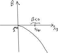
Figure 2: The beta function when . The critical coupling occurs in a region where the beta function is negative. The extremum of the effective potential found there is stable. The coupling constant flow will then be cutoff in the infrared by the condensate itself which gaps the fermion spectrum. The mass of the scalar field is estimated from the curvature of the effective potential at this solution which is of order or times the fermion mass squared111Both and can be arbitrarily small while holding of order one and large enough to be in this regime. , rather than order one as it could be when the curvature had its more natural magnitude .
-
2.
When : There is an infrared fixed point at and an ultraviolet fixed point at . As depicted in figure 3, the ultraviolet fixed point occurs at sufficiently weak coupling that the critical coupling is on the strong coupling side of that fixed point. The beta function is negative in the vicinity of the critical coupling. The extremum of the effective potential found there is stable.
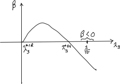
Figure 3: The beta function when has an infrared fixed point and an ultraviolet fixed point as depicted. The ultraviolet fixed point occurs at sufficiently weak coupling that the critical coupling is on the strong coupling branch. In this case the beta function is negative in a region near the critical coupling. The extremum of the effective potential found there is stable. -
3.
When : The beta function has an infrared fixed point at zero and a nontrivial ultraviolet fixed point at a positive value of . As depicted in figure (4), in this case the critical coupling occurs between the two fixed points in a region where the beta function is positive. This means that the extremum of the potential that we find that is located near the critical coupling is a local maximum, rather than minimum. The stable phase is one with runaway condensate where flows to the ultraviolet fixed point. One can check that the effective potential is negative there. There is also a metastable solution with . Thus we conclude that, when , which includes , the case of exactly three dimensions, the theory is unstable.

Figure 4: The beta function when . The critical coupling occurs between the infrared and the ultraviolet fixed points, where the beta function is positive. The theory is unstable in this case.
In conclusion, we emphasize that, like the deformation of the critical Gross-Neveu model that we are discussing is accessible by the large expansion, for any value of between zero and one, although we analyze it only in the large expansion where is of the order of or less than . However, when we restrict ourselves to -perturbatively renormalizable quantum field theory, we obtain a stable well defined theory only for those values of and for which the deformation is marginally relevant. Increasing helps in that it tends to make the operator more relevant. The interactions of the theory – nonlinear effects – tend to make the operator less relevant. If wins this competition, we find a very nice structure. The scalar field obtains a condensate, whose value becomes the fermion mass gap. And a natural flatness of the potential give the fluctuations of the condensate a parametrically small mass times the fermion mass. If loses this competition, the theory is unstable. Its solution has the fermion mass gap going to infinity. There is a metastable solution with condensate zero and massless fermions which, however has a rather low barrier to its decay.
Our analysis of the theory relies on the assumption that counter-terms can be added to the action so that the radiatively induced fermion mass, scalar field tadpole and the quadratic term are canceled at each order of perturbation theory. This is indeed the case in our explicit computation up to order where we see the nontrivial fact that the scalar field tadpole is entirely of the form constant and not constant which would not qualify to be eliminated by a local counter-term which must be analytic in . We expect that this good behaviour persists to higher orders, which would be needed for the model to be renormalizable. It would be interesting to see whether one could develop an all-orders argument that this theory can be renormalized by analytic relevant and marginal counterterms only.
Finally, we have confirmed independently of our renormalization of the corrections to the effective potential, that in the same order of perturbation theory, the wave-function renormalization counterterms that we have used are indeed the appropriate ones to renormalize the Yukawa vertex and the counterterms renormalizing the coupling are indeed what is needed to remove the ultraviolet singularities from the scalar 3 point function. We do not include the details here as they are a very straightforward exercise to reproduce.
The authors acknowledge financial support of the Natural Sciences and Engineering Research Council of Canada.
References
- (1) W. A. Bardeen, C. N. Leung and S. T. Love, “The Dilaton and Chiral Symmetry Breaking,” Phys. Rev. Lett. 56, 1230 (1986).
- (2) K. i. Kondo, H. Mino and K. Yamawaki, “Critical Line and Dilaton in Scale Invariant QED,” Phys. Rev. D 39, 2430 (1989).
- (3) W. D. Goldberger, B. Grinstein and W. Skiba, “Distinguishing the Higgs boson from the dilaton at the Large Hadron Collider,” Phys. Rev. Lett. 100, 111802 (2008) [arXiv:0708.1463 [hep-ph]].
- (4) B. Bellazzini, C. Csaki, J. Hubisz, J. Serra and J. Terning, “A Higgslike Dilaton,” Eur. Phys. J. C 73, no.2, 2333 (2013) [arXiv:1209.3299 [hep-ph]].
- (5) T. Appelquist, J. Ingoldby and M. Piai, “Dilaton Effective Field Theory,” Universe 9, no.1, 10 (2023) [arXiv:2209.14867 [hep-ph]].
- (6) R. Zwicky, “QCD with an Infrared Fixed Point and a Dilaton,” [arXiv:2312.13761 [hep-ph]].
- (7) J. Ingoldby [Lattice Strong Dynamics], “Hidden Conformal Symmetry from Eight Flavors,” [arXiv:2401.00267 [hep-lat]].
- (8) L. Del Debbio and R. Zwicky, “Dilaton and massive hadrons in a conformal phase,” JHEP 08, 007 (2022), [arXiv:2112.11363 [hep-ph]].
- (9) A. Hasenfratz, “Emergent strongly coupled ultraviolet fixed point in four dimensions with eight Kähler-Dirac fermions,” Phys. Rev. D 106, no.1, 014513 (2022), [arXiv:2204.04801 [hep-lat]].
- (10) T. Appelquist et al. [LSD], “Hidden conformal symmetry from the lattice,” Phys. Rev. D 108, no.9, 9 (2023), [arXiv:2305.03665 [hep-lat]].
- (11) G. W. Semenoff and F. Zhou, “Dynamical violation of scale invariance and the dilaton in a cold Fermi gas,” Phys. Rev. Lett. 120, no.20, 200401 (2018), [arXiv:1712.00119 [cond-mat.quant-gas]].
- (12) G. W. Semenoff, “Dilaton in a cold Fermi gas,” [arXiv:1808.03861 [cond-mat.quant-gas]].
- (13) C. Cresswell-Hogg and D. F. Litim, “Line of Fixed Points in Gross-Neveu Theories,” Phys. Rev. Lett. 130, no.20, 201602 (2023), [arXiv:2207.10115 [hep-th]].
- (14) C. Cresswell-Hogg and D. F. Litim, “Critical fermions with spontaneously broken scale symmetry,” Phys. Rev. D 107, no.10, L101701 (2023), [arXiv:2212.06815 [hep-th]].
- (15) R. Zwicky, “The Dilaton Improves Goldstones,” [arXiv:2306.12914 [hep-th]].
- (16) D. F. Litim, N. Riyaz, E. Stamou and T. Steudtner, “Asymptotic safety guaranteed at four-loop order,” Phys. Rev. D 108, no.7, 076006 (2023) [arXiv:2307.08747 [hep-th]].
- (17) C. Cresswell-Hogg and D. F. Litim, “Scale Symmetry Breaking and Generation of Mass at Quantum Critical Points,” [arXiv:2311.16246 [hep-th]].
- (18) A. Pomarol and L. Salas, “Exploring the conformal transition from above and below,” [arXiv:2312.08332 [hep-ph]].
- (19) D. Nogradi and B. Ozsvath, “Dilaton in scalar QFT: a no-go theorem in 4-epsilon and 3-epsilon dimensions,” SciPost Phys. 12, no.5, 169 (2022) [arXiv:2109.09822 [hep-th]].
- (20) R. D. Pisarski, “Fixed Point Structure of (Phi**6) in Three-dimensions at Large N,” Phys. Rev. Lett. 48, 574-576 (1982)
- (21) W. A. Bardeen, M. Moshe, and M. Bander, “Spontaneous Breaking of Scale Invariance and the Ultraviolet Fixed Point in O(N) Symmetric ( in Three-Dimensions) Theory,” Phys. Rev. Lett. 52 (1984) 1188.
- (22) H. Omid, G. W. Semenoff and L. C. R. Wijewardhana, “Light dilaton in the large tricritical model,” Phys. Rev. D 94, no.12, 125017 (2016) [arXiv:1605.00750 [hep-th]].
- (23) S. R. Coleman and E. J. Weinberg, “Radiative Corrections as the Origin of Spontaneous Symmetry Breaking,” Phys. Rev. D 7, 1888-1910 (1973).
- (24) A. J. Niemi and G. W. Semenoff, “Axial Anomaly Induced Fermion Fractionization and Effective Gauge Theory Actions in Odd Dimensional Space-Times,” Phys. Rev. Lett. 51, 2077 (1983).
- (25) A. N. Redlich, “Gauge Noninvariance and Parity Violation of Three-Dimensional Fermions,” Phys. Rev. Lett. 52, 18 (1984).
- (26) A. N. Redlich, “Parity Violation and Gauge Noninvariance of the Effective Gauge Field Action in Three-Dimensions,” Phys. Rev. D 29, 2366-2374 (1984).