Variation of Fundamental Constants due to an Interaction with Ultralight Dark Matter and Constraints on the Yukawa-type Interactions mediated by Scalar Particles

Abstract

An interaction with scalar or pseudoscalar (axion) dark matter may cause the space-time variation of fundamental constants, and atomic spectroscopy provides us with a method of detecting these effects. In this paper, we study the effects produced by an oscillating nuclear mass $m_{N}$ and nuclear radius $r_{N}$ in two transition ratios: the comparison of the two-photon transition in atomic Hydrogen to the results from clocks based on the hyperfine transition in ¹³³Cs, and the ratio of the two optical clock frequencies in Al⁺ and Hg⁺. The sensitivity of these frequencies ratios to changes in the nuclear mass $m_{N}$ and the nuclear radius $r_{N}$ allows us to extract, from experimental data, new limits on the variations of the proton mass, the quark mass, the QCD parameter $\theta$ and the interaction with axion dark matter. We also consider the Yukawa-type scalar field produced by the interaction of feebly interacting hypothetical scalar particles with Standard Model particles in the presence of massive bodies such as the Sun and the Moon. Using the data from the Al⁺/Hg⁺, Yb⁺/Cs and Yb⁺(E2)/Yb⁺(E3) transition frequency ratios, we place constraints on the Yukawa-type interaction of the scalar field with photons, nucleons and electrons, for a range of scalar particle masses. We also consider limits on the Einstein Equivalence Principle (EEP) violating term ($c_{00}$) in the Standard Model Extension (SME) Lagrangian and the dependence of fundamental constants on gravity.

I Introduction

One of the most interesting unsolved problems in modern physics is uncovering the nature of dark matter. Amongst other things, it is hypothesised that dark matter is made up of light bosonic particles, which are not accounted for in the standard model of elementary particles. The candidate particles in this class are the pseudoscalar axion (and axion like particles) and the dilaton-like scalar particle [1, 2, 3]. If the mass of the cold dark matter is very light ($m_{\text{DM}}\ll 1\ \text{eV}$), it may be considered to be a classical field oscillating harmonically at every particular point in space. For axions, we may write this as

$$a=a_{0}\cos(\omega t+\varphi),\ \omega\approx m_{a}\,,$$ (1)

where $\varphi$ is a (position-dependent) phase and $m_{a}$ is the mass of the axion. Assuming that axions saturate the entire dark matter density, the amplitude $a_{0}$ may be expressed in terms of the local dark matter density $\rho_{\text{DM}}\approx 0.4\ \text{GeV/cm}^{3}$, see e.g. Ref. [4],

$$a_{0}=\frac{\sqrt{2\rho_{\text{DM}}}}{m_{a}}\,.$$ (2)

Similar expressions are used to describe the case of a scalar field dark matter $\phi$.

The effects of the interaction between scalar field dark matter and fermions may be presented as the apparent variation of fermion masses. This immediately follows from a comparison of the interaction of a fermion with the scalar field $-g_{f}M_{f}\phi^{n}\bar{\psi}\psi$ and the fermion mass term in the Lagrangian $-M_{f}\bar{\psi}\psi$. Adding these terms gives $M^{\prime}_{f}=M_{f}(1+g_{f}\phi^{n})$, $n=1,2$. Similarly, the interaction of scalar dark matter with the electromagnetic field may be accounted for as a variable fine structure constant $\alpha^{\prime}=\alpha(1+g_{\gamma}\phi^{n})$, see, e.g., Refs. [5, 6]. Note that the variation of quark and electron masses and the variation of the fine structure constant $\alpha$ are determined by different interaction constants and may be treated as independent effects.

These variations may manifest themselves as oscillations of frequencies of atomic clocks [5, 7]. The dependence of atomic transition frequencies on $\alpha$ and the quark masses has been calculated in Refs. [8, 9, 10, 11, 12, 13], and atomic spectroscopy methods have previously been used to place improved limits on the interaction strength of the low mass scalar field dark matter $\phi$ with photons, electrons and quarks by up to 15 orders in magnitude [6, 14]. The experimental results have been obtained by measuring the oscillating frequency ratios of electron transitions in a range of systems, including Dy/Cs [15], Rb/Cs [16], Yb/Cs [17], Sr/H/Si cavity [18], Cs/cavity [19], Cs/H [20], Al⁺/Hg⁺ [21] and Yb⁺/Yb⁺/Sr [22, 23].

Note that if the interaction is quadratic in $\phi$, the scalar field becomes interchangeable with the pseudoscalar (axion) field as $\phi^{2}$ always has positive parity [6]. The corresponding theory has been developed in Ref. [24], in which limits on the axion interaction from atomic spectroscopy experiments were obtained (see also Ref. [25, 26]).

Scalar particles can mediate Yukawa-type interactions between Standard Model particles. A range of experimental methods have been used to constrain these interactions, some of which include Equivalence Principle tests via Torsion Pendulum experiments [27, 28], Lunar Laser Ranging [29] and Atom Interferometry [30]. Another method of constraining these interactions is via atomic spectroscopy measurements. The Yukawa-type scalar field is produced by massive bodies and causes the variation of fundamental constants, leading to a variation in the ratio of transition frequencies. Such calculations and measurements have been performed in Ref. [31].

This paper is divided into three parts. In the first part, we seek to obtain limits on the variation of fundamental constants and subsequently probe ultralight dark matter’s coupling to nuclei. The variation of nuclear parameters affects electronic transitions, and the results of the measurements of the variation in the ratio of transition frequencies in Cs/H [20] and the ratio of optical clocks transitions in Al⁺/Hg⁺ [21] allow us to place constraints on the variation of the proton mass $m_{p}$, the variation of the average quark mass $m_{q}=(m_{u}+m_{d})/2$ and the variation of the nuclear charge radius $r_{N}$ and nuclear mass $m_{N}$, all of which may directly be used to place limits on the QCD axion. The idea that the dependence of the electronic atomic transition frequencies on the nuclear radius (and subsequently on the hadronic parameters above) may be used in the search for dark matter fields was first proposed in Ref. [22]. In this paper, we employ a similar method to Ref. [32], in which the sensitivity the optical clock transitions in Yb⁺ to the variation in the nuclear radius was used to place constraints on the variation of the hadron and quark masses, the QCD parameter $\theta$ and the interaction with axion dark matter.

In the second part we consider the beyond-standard-model effects of gravity such as the Einstein Equivalence Principle (EEP) violating term ($c_{00}$) in the Standard Model Extension (SME) Lagrangian [33] and the dependence of fundamental constants on the gravitational potential.

In the third part we consider the effects produced by the Yukawa-type interaction between hypothetical scalar particles and standard model particles in the presence of massive bodies. Such effects have previously been considered in Ref. [31]. The Yukawa-type scalar field, produced by the Sun and the Moon, affects the fine structure constant $\alpha$ and the fermion mass $m_{f}$. We perform calculations using the measurement of the variation in the ratio of clock transition frequencies Al⁺/Hg⁺ in Ref. [21], Yb⁺/Cs in Ref. [34] and Yb⁺(E2)/Yb⁺(E3) in Ref. [23] to determine limits on the interactions between this scalar field and standard model particles for a range of scalar particle masses.

Note that when discussing the variation of dimensionful parameters, we must be mindful of the units they are measured in, as these units may also vary. In other words, we should consider the variation of dimensionless parameters which have no dependence on any measurement units. Nuclear properties depend on the quark mass and $\Lambda_{\text{QCD}}$. In this work, we keep $\Lambda_{\text{QCD}}$ constant, meaning our calculations measure the variation of a dimensionless parameter $X_{q}\equiv m_{q}/\Lambda_{\text{QCD}}$. As a result, we measure the quark mass in units of $\Lambda_{\text{QCD}}$ - see Refs. [35, 36, 11]. A similar choice of units is assumed for the variation of hadron masses.

In this paper, we assume natural units $\hbar=c=1$ if $\hbar$ and $c$ are not explicitly presented.

II Frequency shift due to isotopic shift

The total electronic energy $E_{\text{tot}}$ of an atomic state contains the energies associated with the finite mass of the nucleus $m_{N}$ (mass shift, MS) and the non-zero nuclear charge radius $r_{N}$ (field shift, FS). These are parametrised as [37]

$$E_{\text{MS}}\approx K_{\text{MS}}\frac{1}{m_{A}}\propto\frac{1}{A}\ \text{and}\ E_{\text{FS}}\approx K_{\text{FS}}r_{N}^{2}\propto A^{2/3}\,,$$ (3)

where $K_{\text{MS}}$ and $K_{\text{FS}}$ are the mass and field shift coefficients respectively and $m_{A}$ is the mass of an atom with atomic mass number $A$, which is largely determined by the nuclear mass $m_{N}$. The variation of the total electronic energy associated with the nuclear degrees of freedom can be written as [38]

$$\frac{\delta E_{\text{tot}}}{E_{\text{tot}}}=-\frac{E_{\text{MS}}}{E_{\text{tot}}}\frac{\delta m_{N}}{m_{N}}+\frac{E_{\text{FS}}}{E_{\text{tot}}}\frac{\delta r_{N}^{2}}{r_{N}^{2}}\,.$$ (4)

The mass shift term dominates for light nuclei whilst the field shift term dominates for heavy nuclei. In general, comparing the electronic transition frequencies $\nu_{a}$ and $\nu_{b}$ of two different atomic species, we obtain

$$\frac{\delta(\nu_{a}/\nu_{b})}{(\nu_{a}/\nu_{b})}=(K_{1}-K_{2})\frac{\delta r_{N}^{2}}{r_{N}^{2}}+(K_{3}-K_{4})\frac{\delta m_{N}}{m_{N}}\,,$$ (5)

where

$$K_{1} =\frac{K_{\text{FS}}^{\nu_{a}}r_{N,a}^{2}}{\nu_{a}}\,,$$ (6)

$$K_{2} =\frac{K_{\text{FS}}^{\nu_{b}}r_{N,b}^{2}}{\nu_{b}}\,,$$ (7)

$$K_{3} =\frac{K_{\text{MS}}^{\nu_{a}}}{\nu_{a}m_{N,a}}\,,$$ (8)

$$K_{4} =\frac{K_{\text{MS}}^{\nu_{b}}}{\nu_{b}m_{N,b}}\,.$$ (9)

III Limits on the linear drift of the QCD parameter $\theta$ and particle masses

In this section, we use the above theory along with experimental observations of the drift in atomic transition frequencies to place limits on the variation of quark and hadronic parameters. Standard model spinor fields $\psi$, photon $F_{\mu\nu}$ and gluon $G^{l}_{\mu\nu}$ fields can have the following interaction vertices with a pseudoscalar field $a$:

$$V=\frac{C_{f}}{f_{a}}\partial_{\mu}a\bar{\psi}\gamma_{5}\gamma^{\mu}\psi+C_{\gamma}\frac{a}{f_{a}}\tilde{F}^{\mu\nu}F_{\mu\nu}+C_{g}\frac{a}{f_{a}}\tilde{G}^{l\,\mu\nu}G^{l}_{\mu\nu}\,.$$ (10)

Here $C_{f}$, $C_{\gamma}$ and $C_{g}$ are dimensionless constants which are of order $O(1)$ for the QCD axion model, but are arbitrary for the general pseudoscalar (axion-like) particle. In particular, upon the substitution $C_{g}=g^{2}/(32\pi^{2})$, or

$$\theta=\frac{32\pi^{2}C_{g}a}{g^{2}f_{a}}\,$$ (11)

the last term in Eq. (10) reduces to the standard QCD $\theta$-term

$$\frac{g^{2}\theta}{32\pi^{2}}\tilde{G}^{l\,\mu\nu}G^{l}_{\mu\nu}\,,$$ (12)

where $\theta=a/f_{a}$, $f_{a}$ is the axion decay constant, $g$ is the strong interaction coupling constant, $G^{l}_{\mu\nu}$ is the gluon field strength and $\tilde{G}^{l\,\mu\nu}$ is its dual. Thus, the classical axion dark matter field $a=a_{0}\cos(m_{a}t+\varphi)$ may be interpreted as a dynamical QCD parameter $\theta=a/f_{a}$.

Let us first consider the variation of fundamental constants due to the variation of the ratio of transition frequencies in Cs/H. Ref. [20] compared results of the variation in the $\ket{1^{2}S_{1/2},F=1,m_{F}=\pm 1}\rightarrow\ket{2^{2}S_{1/2},F^{\prime}=1,m_{F}^{\prime}=\pm 1}$ two-photon transition in atomic hydrogen to results from clocks based on ¹³³Cs in order to deduce limits on the fractional time variation of the fine structure constant $\alpha$. The comparison of the transition in H against the ground state hyperfine transition in ¹³³Cs gives the following fractional time variation [20]

$$\frac{\delta(\nu_{\text{Cs}}/\nu_{\text{H}})}{(\nu_{\text{Cs}}/\nu_{\text{H}})}=3.2\ (6.3)\times 10^{-15}\ \text{yr}^{-1}\,.$$ (13)

The variation of this ratio may be related to the variation of fundamental constants - see Ref. [11]

$$\frac{\delta(\nu_{\text{Cs}}/\nu_{\text{H}})}{(\nu_{\text{Cs}}/\nu_{\text{H}})}=2.83\frac{\delta\alpha}{\alpha}+0.009\frac{\delta m_{q}}{m_{q}}+\frac{\delta(m_{e}/m_{p})}{(m_{e}/m_{p})}\,.$$ (14)

The relative variation of the electron to proton mass ratio can be described as [39]

$$\frac{\delta(m_{e}/m_{p})}{(m_{e}/m_{p})}=-0.037\frac{\delta m_{q}}{m_{q}}-0.011\frac{\delta m_{s}}{m_{s}}+\frac{\delta m_{e}}{m_{e}}\,,$$ (15)

where $m_{s}$ is the mass of the strange quark. For brevity, we may assume that $\delta m_{s}/m_{s}=\delta m_{q}/m_{q}$. Combining these expressions gives

$$\frac{\delta(\nu_{\text{Cs}}/\nu_{\text{H}})}{(\nu_{\text{Cs}}/\nu_{\text{H}})}=2.83\frac{\delta\alpha}{\alpha}-0.039\frac{\delta m_{q}}{m_{q}}+\frac{\delta m_{e}}{m_{e}}\,.$$ (16)

Therefore, using this expression along with the limit presented in Eq. (13), we may obtain a limit on the variation of the quark mass $m_{q}$ assuming that there is no variation of $\alpha$ and $m_{e}$

$$\frac{\delta m_{q}}{m_{q}}=-8.2\ (16)\times 10^{-14}\ \text{yr}^{-1}\,.$$ (17)

When considering the variation of the QCD parameter $\theta$, it is convenient to consider the problem at the hadron level, rather than the quark level. Using the calculations presented in Ref. [11] and the limit (13) we obtain

$$\frac{\delta m_{\pi}}{m_{\pi}} =-4.1\ (8.0)\times 10^{-14}\ \text{yr}^{-1}\,.$$ (18)

Using this value, along with the following result from Ref. [24]

$$\frac{\delta m_{p}}{m_{p}}=0.13\frac{\delta m_{\pi}}{m_{\pi}}\,,$$ (19)

we may subsequently place limits on the drift of the proton mass

$$\frac{\delta m_{p}}{m_{p}}=-5.3\ (10)\times 10^{-15}\ \text{yr}^{-1}\,.$$ (20)

Finally, we may use the relation between the variation of the pion mass and the QCD parameter $\theta$, presented in Ref. [40], to place limits on the linear drift of $\theta$. The pion mass has dependence on $\theta$, and the shift of the pion mass due to a small $\theta$ relative to the pion mass for $\theta=0$ is given by [40]:

$$\frac{\delta m_{\pi}}{m_{\pi}} =-0.05\ \theta^{2}\,$$ (21)

Thus, substituting the value for the drift of the pion mass from Equation (18) yields

$$\frac{d\theta^{2}}{dt} =8.2\ (16)\times 10^{-13}\ \text{yr}^{-1}\,.$$ (22)

We may also perform a similar calculation using measurements from a different ratio of transition frequencies. The drift of the ratio of the optical clock transition frequencies of aluminium and mercury has been measured in Ref. [21]. This drift was used to place limits on the temporal variation of the fine structure constant. Using a similar method to that above, this result may be repurposed to extract limits on the variation of the nuclear radius and hadronic parameters. The rate of change in the ratio of the transition frequencies of ${}^{1}S_{0}\rightarrow\ ^{3}P_{0}$ transitions in Al⁺ and ${}^{2}S_{1/2}\rightarrow\ ^{2}D_{5/2}$ transitions in Hg⁺ was found to be [21]

$$\frac{\delta(\nu_{\text{Al}^{+}}/\nu_{\text{Hg}^{+}})}{{\nu_{\text{Al}^{+}}}/\nu_{\text{Hg}^{+}}}=-5.3\ (7.9)\times 10^{-17}\ \text{yr}^{-1}\,.$$ (23)

Once again we note the fact that mass shift dominates the isotope shift effects in light elements, while field (volume) shift dominates in heavy elements. As such, the isotopic shift in $\text{Al}^{+}$ is dominated by the mass shift component, while the isotopic shift in $\text{Hg}^{+}$ is dominated by the field shift component.

The mass shift is divided into two components: the normal mass shift (NMS) and the specific mass shift (SMS). The NMS results from a change in the reduced electron mass, and its parameter is easily calculated from the transition frequency

$$K_{\text{NMS}}^{\nu}=-\frac{\nu}{1822.888}\ \text{amu}\,,$$ (24)

where the factor in the denominator refers to the ratio of the atomic mass unit to the electron mass. Using the transition frequency from the experimental observation of the ${}^{1}S_{0}\rightarrow\ ^{3}P_{0}$ transition in ²⁷Al⁺ of Ref. [41], we calculate the normal mass shift factor in Al⁺ to be $K_{\text{NMS}}^{\nu_{\text{Al}^{+}}}=-615$ GHz amu. Using the calculated ratio of the specific to normal mass shifts from Ref. [42], we yield a total mass shift parameter of $K_{\text{MS}}^{\nu_{\text{Al}^{+}}}=-1530$ GHz amu.

Now we must consider the effects from the field shift in Hg⁺. Using the CIPT method (configuration interaction with perturbation theory [43]), which allows us to deal with open shells, and the approach similar to what is described in Ref. [44] we have calculated the field shift parameter for the ${}^{2}S_{1/2}\rightarrow\ ^{2}D_{5/2}$ transition in Hg⁺ to be $85.5$ GHz/fm². This value is in agreement with the theoretical calculations of the isotope shift in Hg⁺ presented in Ref. [45]. Thus, using the MS and FS parameters along with Eq. (5), we obtain

$$\begin{split}\frac{\delta(\nu_{\text{Al}^{+}}/\nu_{\text{Hg}^{+}})}{{\nu_{\text{Al}^{+}}}/\nu_{\text{Hg}^{+}}}=-\bigg{[}\frac{K_{\text{FS}}^{\nu_{\text{Hg}^{+}}}r_{N,\text{Hg}^{+}}^{2}}{\nu_{\text{Hg}^{+}}}\frac{\delta r_{0}^{2}}{r_{0}^{2}}+\\ \frac{K_{\text{MS}}^{\nu_{\text{Al}^{+}}}}{\nu_{\text{Al}^{+}}m_{N,\text{Al}^{+}}}\frac{\delta m_{N}}{m_{N}}\bigg{]}\,.\end{split}$$ (25)

Here, we have used the fact that the nuclear radii in all nuclei may be quite accurately related to the internucleon distance $r_{0}$ by the universal formula $r_{N}=A^{1/3}r_{0}$. This implies that these quantities have equivalent fractional variations. Presenting limits on the variation of $r_{0}$ is more useful as it allows one to compare the results of measurements in different nuclei. Noting that $r_{N,\text{Hg}^{+}}^{2}=5.4474$ fm in ¹⁹⁹Hg [46] and $m_{N,\text{Al}^{+}}\approx 27m_{p}$ in ²⁷Al, we yield the following limits

$$\frac{\delta r_{0}}{r_{0}} =-1.1\ (1.7)\times 10^{-14}\ \text{yr}^{-1}\,,$$ (26)

$$\frac{\delta m_{p}}{m_{p}} =1.0\ (1.6)\times 10^{-12}\ \text{yr}^{-1}\,.$$ (27)

Considering these effects as separate sources of the variation allows us to derive independent limits on the variation of quark and hadronic parameters.

Firstly, using a similar method to the one presented in Ref. [32], we consider the effects arising from a variation in the internucleon distance $r_{0}$. Calculations of the dependence of nuclear energy levels and nuclear radii on fundamental constants were performed in Refs. [35, 47, 36]. Specifically, in Table VI of Ref. [36], the sensitivity coefficients of nuclear radii to the variation of hadron masses for several light nuclei have been presented. These results may be extended to all nuclei due to the relation $r_{N}=A^{1/3}r_{0}$, meaning it is sufficient to calculate the dependence of $r_{0}$ in any nucleus. The sensitivity coefficients are defined by the relation

$$\frac{\delta r_{0}}{r_{0}}=\sum_{h}K_{h}\frac{\delta m_{h}}{m_{h}}\,.$$ (28)

The sum over hadrons in Refs. [47, 36] includes contributions from $\pi$, nucleon, $\Delta$ and vector mesons (these hadron masses are parameters of the kinetic energy and nucleon interaction operators used in Refs. [47, 36]). The sensitivity to the pion mass is given by the coefficient $K_{\pi}=1.8$ and the sensitivity to the nucleon mass is given by $K_{n}=-4.8$. We neglect contributions from $\Delta$ and vector mesons as they are of a similar magnitude with opposing sign, meaning their resulting contribution is small and unstable.

Subsequently, the variation of hadron masses may be related to variation of the quark mass, see e.g. Ref. [48]:

$$\frac{\delta m_{h}}{m_{h}}=K_{h,q}\frac{\delta m_{q}}{m_{q}}\,,$$ (29)

where $m_{q}=(m_{u}+m_{d})/2$ corresponds to the average light quark mass. The sensitivity coefficient for the pion mass is an order of magnitude bigger than that for other hadrons since the pion mass vanishes for zero quark mass ($m_{\pi}\propto m_{q}^{1/2}$) while other hadron masses remain finite. Indeed, according to Refs. [49, 50] $K_{\pi,q}=0.498$ for the pion, while $K_{n,q}=0.06$ for nucleons. The sensitivity coefficients to the quark mass have been calculated for light nuclei in Ref. [36]. The average value is given by

$$\frac{\delta r_{0}}{r_{0}}=0.3\frac{\delta m_{q}}{m_{q}}\,.$$ (30)

We note that here there are partial cancellations of different contributions, so the sensitivity is smaller than that following from pion mass alone. Refs. [47, 36] have also presented calculations of the dependence of the nuclear energies and radii on the variation of the fine structure constant $\alpha$. Applying Equation (30) to the limit on the variation of the internucleon distance presented in (26), we determine limits on the variation of the quark mass to be

$$\frac{\delta m_{q}}{m_{q}}=-3.7\ (5.7)\times 10^{-14}\ \text{yr}^{-1}\,.$$ (31)

Once again, in order to place limits on the variation of the proton mass and the QCD parameter $\theta$, it is convenient to consider the problem at the hadron level, rather than the quark level. In Ref. [36], the sensitivity of the nuclear radius to the masses of the pion, nucleon, vector meson and delta has been calculated. In the following estimate, we do not include contributions from the vector meson and delta as their contributions are smaller. These contributions also have opposing signs, meaning they partially cancel each other out making their contribution less reliable. The variation of the nuclear radius may be written in terms of the pion and nucleon mass as

$$\frac{\delta r_{0}}{r_{0}}=1.8\frac{\delta m_{\pi}}{m_{\pi}}-4.8\frac{\delta m_{n}}{m_{n}}=1.2\frac{\delta m_{\pi}}{m_{\pi}}\,,$$ (32)

where in the last equality we have applied Equation (19). Thus, once again applying Equation (26), we obtain a limit on the drift of the pion mass

$$\frac{\delta m_{\pi}}{m_{\pi}}=-9.2\ (14)\times 10^{-15}\ \text{yr}^{-1}\,.$$ (33)

Finally, we apply Equation (21) in order to place constraints on the linear drift of the QCD parameter $\theta$

$$\frac{d\theta^{2}}{dt}=1.8\ (2.8)\times 10^{-13}\ \text{yr}^{-1}\,.$$ (34)

These limits are approximately 44 times weaker than the limits imposed from the sensitivity of the optical clock transitions in Yb⁺ obtained in Ref. [32]. This difference corresponds exactly to the difference in the accuracy of the experimental measurements of the variation in clock frequency ratios, showing that these systems have equivalent sensitivities to the variation of the internucleon distance. We however note that the limits from the Al⁺/Hg⁺ clock ratio are $\sim 2-4$ times stronger than those calculated for the Cs/H system, despite the fact that the accuracy of the Al⁺/Hg⁺ measurements is $\sim 60$ times better. This implies that the sensitivity of the Cs/H ratio to changes in the hadron constants is higher than that of the Al⁺/Hg⁺ ratio.

Let us now consider the effects arising from a variation of the nuclear mass $m_{N}$. The nuclear mass may be related to the proton mass $m_{p}$ by the following relation $m_{N}\approx A\ m_{p}$. As such, these parameters have equivalent fractional variations, meaning the limit from Eq. (27) applies. Using this result, along with the relation between the pion and the proton mass presented in Equation (19), we may place limits on the drift of the pion mass

$$\frac{\delta m_{\pi}}{m_{\pi}}=8.1\ (12)\times 10^{-12}\ \text{yr}^{-1}\,.$$ (35)

Using the calculations presented in Ref. [11], we may use this result to place limits on the variation of the quark mass $m_{q}$

$$\begin{split}\frac{\delta m_{q}}{m_{q}}&=1.6\ (2.4)\times 10^{-11}\ \text{yr}^{-1}\,.\end{split}$$ (36)

We also use the relation between the variation of the pion mass and the QCD parameter $\theta$ presented in Equation (21) to place constraints on the linear drift of $\theta^{2}$

$$\begin{split}\frac{d\theta^{2}}{dt}&=-1.6\ (2.4)\times 10^{-10}\ \text{yr}^{-1}\,.\end{split}$$ (37)

As expected, the limits obtained upon considering the variation in the ratio of frequencies (23) as being due to the drift of the nuclear (and hence nucleon) mass are weaker than the limits from the variation of the internucleon distance.

IV Gravity related variation of fundamental constants

In some theoretical models, atomic transition frequencies and fundamental constants may depend on the gravitational potential. In Ref. [51] limits on the gravity related variation of fundamental constants are derived from measurements of the drift of atomic clock frequency ratios. In a similar way, we may obtain limits on the gravity related variation of the nuclear radius and nuclear mass using the measurement of the variation in the ratio of transition frequencies in $\text{Al}^{+}/\text{Hg}^{+}$ from Refs. [52, 21]. We will also calculate limits on gravity related variation of these quantities for other systems of interest, Yb⁺/Cs [34] and Yb⁺/Yb⁺ [23].

Noting the dependence of the frequency shift on the nuclear mass and radius from Eq. (5), we introduce the parameters $\kappa_{r,N}$ as follows: (see Ref. [51])

$$\frac{\delta r_{N}^{2}}{r_{N}^{2}} =\kappa_{r}\ \delta\left(\frac{GM}{rc^{2}}\right)\,,$$ (38)

$$\frac{\delta m_{N}}{m_{N}} =\kappa_{N}\ \delta\left(\frac{GM}{rc^{2}}\right)\,.$$ (39)

It is instructive to link these parameters $\kappa_{r}$ and $\kappa_{N}$ to the Einstein Equivalence Principle (EEP) violating term in the Standard Model Extension Hamiltonian  [33]. This term may be presented as a correction to the kinetic energy which in non-relativistic form is equal to (see e.g. [53])

$$\delta H=\frac{2}{3}c_{00}\frac{U}{c^{2}}\frac{p^{2}}{2m_{e}},$$ (40)

where $c_{00}$ is a parameter of the Standard Model Extension (SME) Lagrangian [33], $U$ is the gravitational potential, $p$ is the electron momentum operator and $m_{e}$ is the electron mass. Limits on $c_{00}$ have been found by monitoring the drift of atomic clock frequencies for different transitions (see e.g. [52, 53]). Ref. [52] subsequently used the limits on this parameter to determine a limit on the gravity-related variation of the fine structure constant $\kappa_{\alpha}$

$$\frac{\delta\alpha}{\alpha}=\kappa_{\alpha}\ \delta\left(\frac{GM}{c^{2}r}\right)\,,$$ (41)

where in the case of a relative change of two transition frequencies in different atomic species $\delta\omega_{a}/\omega_{a}=K_{\alpha a}(\delta\alpha/\alpha)$ and $\delta\omega_{b}/\omega_{b}=K_{\alpha b}(\delta\alpha/\alpha)$, the parameter $\kappa_{\alpha}$ is equal to

$$\kappa_{\alpha}=\frac{2}{3}\frac{R_{b}-R_{a}}{K_{\alpha a}-K_{\alpha b}}c_{00}\,,$$ (42)

where $R_{a}$ and $R_{b}$ represent the relativistic factors of atoms $a$ and $b$ respectively, which describe the deviation from the expectation value of the kinetic energy of a relativistic atomic electron from the value given by the non-relativistic virial theorem [52]

$$R=-\frac{\Delta E_{i}-\Delta E_{j}}{E_{i}-E_{j}}\,,$$ (43)

where $\Delta E_{i}$ is the energy shift of the state $i$ due to the relativistic kinetic energy operator. In the non-relativistic limit, $R=1$. Thus, we employ a similar method and derive expressions for the parameters $\kappa_{r}$ and $\kappa_{N}$ describing the variation of the nuclear radius and nuclear mass:

$$\kappa_{r} =\frac{2}{3}\frac{R_{b}-R_{a}}{K_{1}-K_{2}}c_{00}\,,$$ (44)

$$\kappa_{N} =\frac{2}{3}\frac{R_{b}-R_{a}}{K_{3}-K_{4}}c_{00}\,,$$ (45)

where $K_{1,2,3,4}$ are defined in Eq. (5). The value of $R$ has been calculated for a number of clock transitions in Ref. [52], see Table 1. Ref. [52] also calculated a limit on the value of the SME parameter $c_{00}$ due to the change in the Sun’s gravitational potential for the ratio of these transition frequencies $\nu_{\text{Al}^{+}}/\nu_{\text{Hg}^{+}}$. As such, we may substitute all known quantities into Eqs. (44, 45) and determine a limit on the gravity related variation of the nuclear radius and nuclear mass. We also use the limits on the coupling to gravity of the fine structure constant $\alpha$, presented in Refs. [34] (Yb⁺/Cs) and [23] (Yb⁺/Yb⁺) in order to place improved limits on gravity’s coupling to the nuclear radius $\kappa_{r}$. In performing these calculations, we make use of the following result for the difference in field shift parameters in the electric octupole (E3) and electric quadrupole (E2) transitions in Yb⁺: $K_{1}-K_{2}=2.4\times 10^{-3}$ [22], and the sensitivity of variations in this ratio to the fine structure constant $\alpha$, $k_{\alpha}(E3)-k_{\alpha}(E2)=-6.95$ [10]. The results are presented in Table 2.

Atom/Ion	Ground state	Clock state	$\hbar\omega\left[\mathrm{cm}^{-1}\right]$	$R$
$\mathrm{Al}^{+}$	$3s^{2}$   ${}^{1}\mathrm{S}_{0}$	$3s3p$  ${}^{3}\mathrm{P}_{0}^{o}$	37393	1.00
$\mathrm{Hg}^{+}$	$5d^{10}6s$ ${}^{2}\mathrm{S}_{1/2}$	$5d^{9}6s^{2}$ ${}^{2}\mathrm{D}_{5/2}$	35515	0.2
$\mathrm{Yb}^{+}$	$6s$   ${}^{2}\mathrm{S}_{1/2}$	$5d$  ${}^{2}\mathrm{D}_{3/2}$	22961	1.48
$\mathrm{Yb}^{+}$	$6s$   ${}^{2}\mathrm{S}_{1/2}$	$4f$   ${}^{2}\mathrm{F}_{7/2}$	21419	-1.9

Table 1: Relativistic factors ($R$) for optical clock transitions in atoms and ions [52].

System	Source	$c_{00}$	$\kappa_{\alpha}$	$\kappa_{r}$	$\kappa_{n}$	$\kappa_{e}$
Al+/ Hg+ [21]	Sun	$-3.0\ (5.7)\times 10^{-7}$ [52]	$5.3\ (10)\times 10^{-8}$ [52]	$-6.7\ (13)\times 10^{-5}$	$-3.1\ (6.0)\times 10^{-3}$	—
	Moon	$-6.0\ (12)\times 10^{-3}$	$1.1\ (2.1)\times 10^{-3}$	-0.67  (1.3)	-63  (120)	—
$\mathrm{Yb}^{+}/\mathrm{Cs}$ [34]	Sun	$4.2\ (3.3)\times 10^{-8}$	$14\ (11)\times 10^{-9}$ [34]	$4.0\ (3.1)\times 10^{-5}$	$7\ (45)\times 10^{-8}$ [34]	$-7\ (45)\times 10^{-8}$ [34]
$\mathrm{Yb}^{+}/\mathrm{Yb}^{+}$ [23]	Sun	$-7.4\ (9.3)\times 10^{-9}$	$-2.4\ (3.0)\times 10^{-9}$[23]	$7.0\ (8.7)\times 10^{-6}$	$2.1\ (2.9)\times 10^{-4}$	—

Table 2: Limits on the Standard Model Extension parameter $c_{00}$ and the parameters $\kappa_{\alpha}$, $\kappa_{r}$, $\kappa_{n}$ and $\kappa_{e}$ describing the dependence of the fine structure constant $\alpha$, the internucleon distance $r_{0}$ (derived from the nuclear charge radius $r_{N}$), the nucleon mass and the electron mass on the gravitational potential.

V Constraints on the Yukawa-type scalar field produced in the presence of massive bodies

In this section, we consider the Yukawa-type scalar field produced in the presence of massive bodies. Let us first provide an introduction to the phenomenology of this scalar field, following Ref. [31]. A scalar field $\phi$ interacts with the standard model sector via the Yukawa-type Lagrangian:

$$\mathcal{L}_{\text{int}}=-\sum_{f}\frac{\phi}{\Lambda_{f}}m_{f}\bar{f}f+\frac{\phi}{\Lambda_{\gamma}}\frac{F_{\mu\nu}F^{\mu\nu}}{4}\,.$$ (46)

Here, the first term represents the coupling to fermion fields $f$, with mass $m_{f}$ and $\bar{f}=f^{\dagger}\gamma_{0}$, while the second term represents the coupling to the photon field. $\Lambda_{f}$ and $\Lambda_{\gamma}$ are new-physics energy scales which determine the strength of these couplings. Adding these interaction terms to the relevant terms in the standard model Lagrangian

$$\mathcal{L}\supset-\sum_{f}m_{f}\bar{f}f-\frac{F_{\mu\nu}F^{\mu\nu}}{4\alpha}\,,$$ (47)

we observe that we may present the effects of the interaction terms in the form of a variable fermion mass $m_{f}$ and electromagnetic fine-structure constant $\alpha$ (see e.g  [7])

$$m_{f} \rightarrow m_{f}\left(1+\frac{\phi}{\Lambda_{f}}\right)\,,$$ (48)

$$\alpha \rightarrow\frac{\alpha}{1-\phi/\Lambda_{\gamma}}\approx\alpha\left(1+\frac{\phi}{\Lambda_{\gamma}}\right)\,.$$ (49)

Adding the kinetic term to the interaction Lagrangian (46) gives the following equations of motion for the field $\phi$:

$$(\partial_{\mu}\partial_{\mu}+m_{\phi}^{2})\phi=-\sum_{f}\frac{m_{f}}{\Lambda_{f}}m_{f}\bar{f}f+\frac{1}{\Lambda_{\gamma}}\frac{F_{\mu\nu}F^{\mu\nu}}{4}\,,$$ (50)

where $m_{\phi}$ is the mass of the scalar particle. This implies that in the presence of the interaction (46), the standard model fermion and photon fields act as sources of the scalar field. Massive bodies such as stars or galaxies, which are composed of atoms, may act as these sources, producing a Yukawa-type scalar field. This field may produce a local variation of fundamental constants in the presence of a massive body with a varying distance to the laboratory. As such, we may investigate the influence of the scalar particle $\phi$ on atomic spectroscopy experiments, see Ref. [31]. In the following subsections we place constraints on the scalar field’s interaction with the Standard Model particles. Specifically, we consider the effects produced by a variation in the scalar field due to both the semi-annual variation in the Sun-Earth distance, and the approximately semi-monthly variation in the Moon-Earth distance.

V.1 Effects produced by the variation in the Sun-Earth distance

Similar to the gravitational potential, the scalar Yukawa potential depends on the distance between Sun and Earth. Assuming the Sun’s elemental composition to be 75% ¹H and 25% ⁴He by mass, the resultant scalar field may be expressed as [31]

$$\phi_{\text{Sun}}=-N_{s}m_{n}\left[\frac{0.15}{\Lambda_{n^{\prime}}}+1.1\biggl{\{}\frac{1}{\Lambda_{p}}+\frac{5\times 10^{-4}}{\Lambda_{e}}\biggr{\}}+\frac{8\times 10^{-4}}{\Lambda_{\gamma}}\right]\frac{e^{-m_{\phi}r}}{4\pi r}=-N_{s}\beta_{s}\frac{e^{-m_{\phi}r}}{4\pi r}\,,$$ (51)

where $m_{n}=(m_{p}+m_{n^{\prime}})/2=0.94$ GeV is the average nucleon mass and $N_{s}$ is the number of atoms inside the Sun. The number of nucleons inside the Sun may be determined as mass of the Sun divided by the proton mass, $N_{s}=M_{s}/m_{p}=1.99\times 10^{30}\ \text{kg}/1.67\times 10^{-27}\ \text{kg}=1.19\times 10^{57}$. The ratio of the number of neutrons and protons depends on the composition of the Sun, which is mainly composed of hydrogen and helium. According to Eq. (51), the average atom in the Sun contains 1.1 protons and 0.15 neutrons, i.e. 1.25 nucleons. This implies that the number of atoms in the Sun is $N_{s}=0.95\times 10^{57}$. In obtaining limits on the nucleon constant $\Lambda_{n}$ we consider the sum of the proton and neutron contributions assuming $\Lambda_{n^{\prime}}=\Lambda_{p}$. In this case, the limits on $\Lambda_{n}$ have no dependence on the composition of the Sun. The Earth’s orbit is elliptical, with the Earth-Sun distance changing between $1.52\times 10^{8}$ km and $1.47\times 10^{8}$ km.

Using new and existing calculations of the variation of fundamental constants due to changes in the Yukawa potential (see Appendix A), we place constraints on the Yukawa-type interactions of the scalar field from the Sun with photons, nucleons and electrons for a range of scalar particle masses, using a similar method to Ref. [31]. Constraints on the parameters $\Lambda_{\gamma},\Lambda_{n}$ and $\Lambda_{e}$ are presented in Figure 1 and summarised in Table 3.

V.2 Effects produced by the variation in the Moon-Earth distance

We may also extract limits on these parameters by considering the varying Yukawa potential of the Moon’s orbit around Earth. Doing so allows one to investigate the coupling at larger values of the scalar particle mass $m_{\phi}$. The average atom in the Moon contains 12 protons and 12 neutrons. Following Ref. [31] we obtain the Moon’s scalar field to be

$$\phi_{\text{Moon}}=-N_{m}m_{n}\left[\frac{12}{\Lambda_{n^{\prime}}}+12\biggl{\{}\frac{1}{\Lambda_{p}}+\frac{5\times 10^{-4}}{\Lambda_{e}}\biggr{\}}+\frac{0.03}{\Lambda_{\gamma}}\right]\frac{e^{-m_{\phi}r}}{4\pi r}=-N_{m}\beta_{m}\frac{e^{-m_{\phi}r}}{4\pi r}\,.$$ (52)

The number of nucleons in the Moon may be determined as the mass of the Moon divided by the proton mass, $N_{m}=M_{m}/m_{p}=7.34\times 10^{22}\ \text{kg}/1.67\times 10^{-27}\ \text{kg}=4.40\times 10^{49}$. The average atom in the Moon contains 24 nucleons. This implies that the number of atoms in the Moon to be $N_{m}=1.8\times 10^{48}$. In obtaining limits on the nucleon constant $\Lambda_{n}$ we once again consider the sum of the proton and neutron contributions assuming $\Lambda_{n^{\prime}}=\Lambda_{p}$. In this case, the limits on $\Lambda_{n}$ have no dependence on the composition of the Moon.

The average Earth-Moon distance is $3.84\times 10^{5}$ km, centre to centre, and this value varies between $3.69\times 10^{5}$ km and $3.99\times 10^{5}$ km with a period of approximately 27.3 days. Furthermore, due to the relatively large diameter of the Earth ($\sim 1.27\times 10^{4}$ km), we note that there is also a daily variation in the distance between the Moon and the laboratory. Despite this, the contributions from the monthly variations are more significant, and as such we consider a variation of $\sim 3.0\times 10^{4}$ km in the Earth-Moon distance, which corresponds to the minimal seasonal variation (see Ref. [31]).

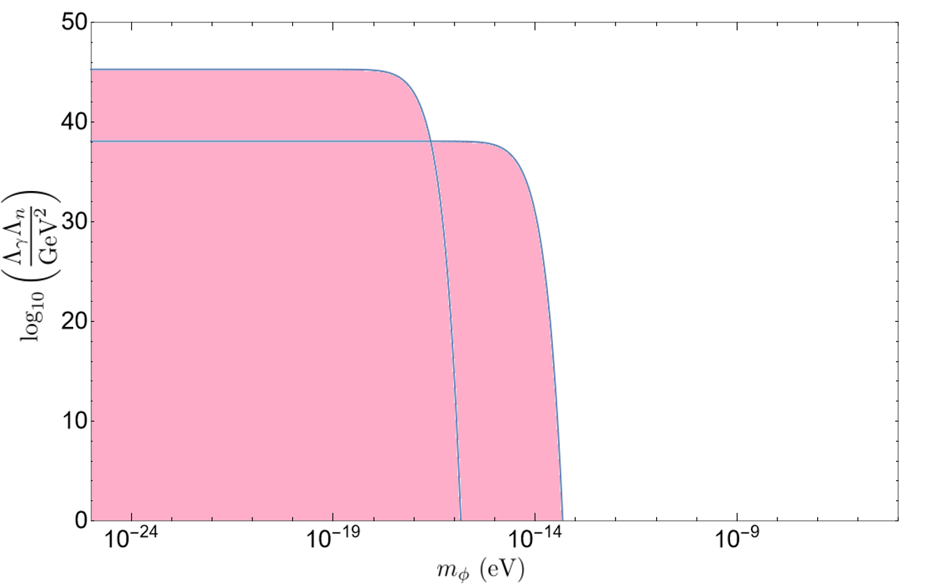
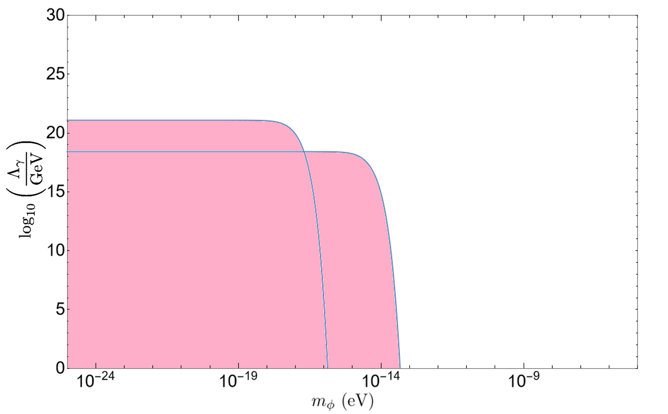
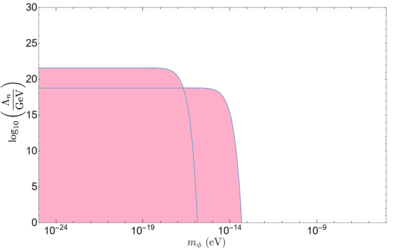
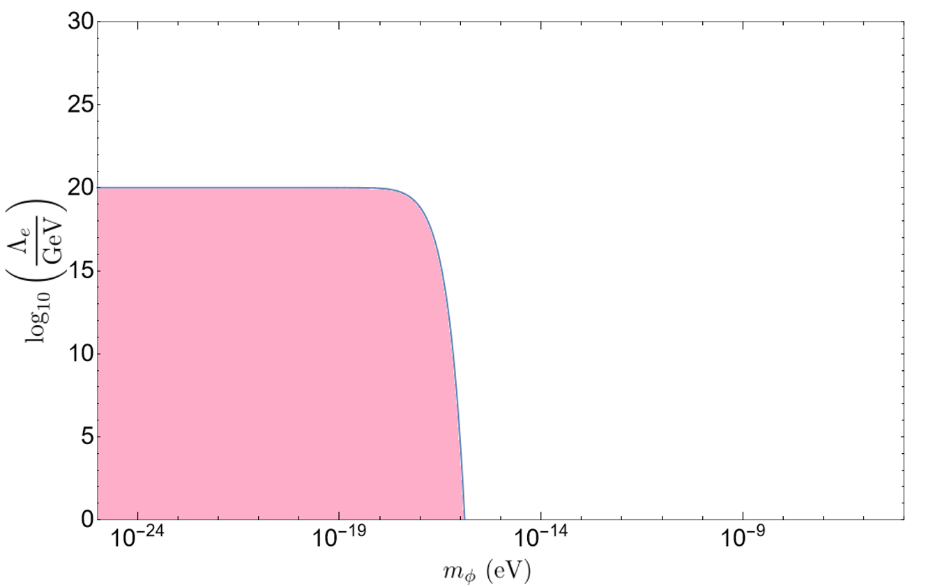
Figure 1: Limits on the constants of the Yukawa-type interaction Eq. (46) of the scalar field $\phi_{s}$ with photons ($\Lambda_{\gamma}$), nucleons ($\Lambda_{n}$) and electrons ($\Lambda_{e}$). In obtaining limits on the nucleon constant $\Lambda_{n}$ we sum the contributions from the proton and neutron coupling constants, assuming $\Lambda_{n^{\prime}}=\Lambda_{p}$. The upper curve depicts the region constrained by the potential of the Sun, whilst the lower and longer curve depicts the region constrained by the Moon’s potential. There is no data for the effect of the Moon’s gravitational potential on the electron interaction constant (lower right tile).

Thus, using a similar method to that of the previous subsection, we may determine limits on the Yukawa-type interaction between the varying scalar field and photons/nucleons for a range of scalar particle masses. Constraints on these parameters are presented in Fig. 1, and summarised in Table 3.

V.3 Limits on combinations of coupling constants

Spectroscopy measurements may also be used to probe different combinations of the couplings constants $\Lambda_{\gamma,p,n,e}$ [31], some of which may not be otherwise probed using anomalous-force measurements. Such results may be useful in the case when the variation of the ratio of optical clock transition frequencies and the source-dependent functions $\beta_{s,m}$ are dominated by different terms. Thus we may use the results of the previous two subsections to provide constraints on the combination of parameters $\Lambda_{\gamma}\Lambda_{n}$, see Figure 1. If the scalar particle’s Compton wave length $\hbar/m_{\phi}c$ is bigger than the distance to the source, we determine the following limits for the combination of parameters $\beta_{s,n}/\Lambda_{\gamma}$

$$\frac{\Lambda_{\gamma}}{\beta_{s}} \gtrsim 2\times 10^{45}\ \text{GeV}^{2}\,,$$ (53)

$$\frac{\Lambda_{\gamma}}{\beta_{m}} \gtrsim 1\times 10^{38}\ \text{GeV}^{2}\,.$$ (54)

System	Source/Attractor	$\Lambda_{\gamma}/\beta$	$\Lambda_{\gamma}$	$\Lambda_{n}$	$\Lambda_{e}$
		(GeV2)	(GeV)	(GeV)	(GeV)
Al+/ Hg+ [21]	Sun	$7\times 10^{43}$	$2\times 10^{20}$	$1\times 10^{21}$	—
	Moon	$1\times 10^{38}$	$2\times 10^{18}$	$6\times 10^{18}$	—
Yb+/ Cs [34]	Sun	$4\times 10^{44}$	$6\times 10^{20}$	$5\times 10^{21}$	$1\times 10^{20}$
Yb+/ Yb+ [23]	Sun	$2\times 10^{45}$	$1\times 10^{21}$	$4\times 10^{21}$	—

Table 3: Lower limits on the constants of the Yukawa-type interaction Eq. (46) of the scalar field $\phi_{s}$ with photons ($\Lambda_{\gamma}$), nucleons ($\Lambda_{n}$) and electrons ($\Lambda_{e}$) in the interval of small scalar field masses determined by the condition that the scalar particle’s Compton wave length $\hbar/m_{\phi}c$ is bigger than the distance to the source, $m_{\phi}<1.0\times 10^{-18}$ eV for the Sun-Earth distance and $m_{\phi}<0.5\times 10^{-15}$ eV for the Moon-Earth distance. In obtaining limits on the nucleon constant $\Lambda_{n}$ we sum the contributions from the proton and neutron coupling constants, assuming $\Lambda_{n^{\prime}}=\Lambda_{p}$. The full exclusion plots are presented in Fig. 1.

Limits on the variation of $\alpha$, the nucleon mass and the electron mass due to the variation of the Sun’s distance to Earth are presented in Table 4. The details are presented in Appendix A.

System	$\delta\alpha/\alpha$	$\delta m_{n}/m_{n}$	$\delta m_{e}/m_{e}$
Al+/ Hg+ [21]	$0.17\ (0.33)\times 10^{-16}$	$1.2\ (2.3)\times 10^{-15}$	—
$\mathrm{Yb}^{+}$/Cs [34]	$4.6\ (3.6)\times 10^{-18}$	$2.3\ (15)\times 10^{-17}$	$-2.3\ (15)\times 10^{-17}$
$\mathrm{Yb}^{+}/\mathrm{Yb}^{+}$ [23]	$-7.9\ (9.9)\times 10^{-19}$	$1.3\ (1.6)\times 10^{-16}$	—

Table 4: Summary of the obtained constraints on the variation of fundamental constants due to changes in the distance to the Sun (interpreted in Refs. [21, 34, 23] as the effect of the variation in the Sun’s gravitational potential).

VI Summary

One of the most effective ways to search for signatures of ultralight dark matter’s interaction with standard model particles is via atomic spectroscopy. Such measurements indicate the potential space-time variations in fundamental constants which may be caused by low mass scalar or pseudoscalar (axion) dark matter fields. In particular, we relate the proton mass $m_{p}$ and the quark mass $m_{q}$ variation to measurements in the variation of two frequency ratios: the comparison of the two-photon transition in atomic Hydrogen to the results from clocks based on ¹³³Cs in Ref. [20], and the variation in the ratio of the two optical clock frequencies in Al⁺ and Hg⁺ in Ref. [21]. We used this data to place new limits on the variation of the proton mass $m_{p}$, as well as independent limits on the variation of the quark mass $m_{q}$, both of which may be used to place limits on the variation of the QCD parameter $\theta$, and on the interaction with scalar and axion dark matter.

In the second part of this paper we considered the beyond-standard-model effects of gravity such as the Einstein Equivalence Principle (EEP) violating term ($c_{00}$) in the Standard Model Extension (SME) Lagrangian [33] and the dependence of fundamental constants on the gravitational potential, based on the measurements of the dependence of the ratio of atomic transition frequencies Al⁺/Hg⁺  [52, 21], Yb⁺/ Cs [34] and Yb⁺/Yb⁺ [23] to the Sun-Earth distance.

In the third part of this paper we considered the Yukawa-type field produced by scalar particles in the presence of massive bodies. We determine limits on the Yukawa-type interactions of the scalar particle with photons, nucleons and electrons for a wide range of scalar particle masses, basing on the measurements of dependence of the ratio of atomic transition frequencies Al⁺/Hg⁺  [52, 21], Yb⁺/ Cs [34] and Yb⁺/Yb⁺ [23] on the Sun-Earth and Moon-Earth distances. If the scalar particle’s Compton wave length $\hbar/m_{\phi}c$ is bigger than the distance to the source, we place the following limits on the coupling constants of the interaction of the scalar field with photons, nucleons and electrons: $\Lambda_{\gamma}\gtrsim 1\times 10^{21}\ \text{GeV}$, $\Lambda_{n}\gtrsim 5\times 10^{21}\ \text{GeV}$ and $\Lambda_{e}\gtrsim 1\times 10^{20}\ \text{GeV}$ .

These limits may be compared to the limits from the atomic spectroscopy measurements presented in Ref. [31]. Our limits based on the Sun and Moon data are significantly stronger. However, Ref. [31] also obtained limits on the scalar field produced by a 300 kg lead mass on a distance of 1 m. This area is sensitive to much bigger scalar masses and is not covered by our results.

Appendix A Coupling of fundamental constants to changes in the Yukawa potential from the Sun/Moon

In this appendix we detail the calculations of the variation of fundamental constants due to changes in the Yukawa potential. We will use experimental data on the variation of atomic transition frequencies as functions of Sun-Earth and Moon-Earth distances motivated by the search for dependence of the fundamental constants on the gravitational potential. Constraints on this dependence were obtained for all the systems of interest: Al⁺/Hg⁺, Yb⁺/Cs and Yb⁺/Yb⁺. The summary is presented in Table 4.

Let us start with the variation of the fine structure constant $\alpha$. Equation (49) implies the following relation

$$\frac{\delta\alpha}{\alpha}=\frac{\delta\phi}{\Lambda_{\gamma}}\,,$$ (55)

At $m_{\phi}\rightarrow 0$ we have from (51) or (52)

$$\delta\phi=-\frac{\beta N_{S,M}}{4\pi}\delta\left(\frac{1}{r}\right)_{S,M}\equiv\beta D_{S,M}.$$ (56)

Here $N_{S,M}$ is number of atoms in the Sun or the Moon ($N_{S}\approx 0.95\times 10^{57}$ and $N_{M}\approx 1.8\times 10^{48}$) and $\delta(1/r)_{S,M}$ is half-yearly variation of the inverted Sun-Earth or Moon-Earth distance. Then

$$\left|\Lambda_{\gamma}/\beta\right|=\left|\frac{D_{S,M}}{\delta\alpha/\alpha}\right|,$$ (57)

and

$$\Lambda_{\gamma}=\sqrt{\left|\frac{m_{n}a_{\gamma}D_{S,M}}{\delta\alpha/\alpha}\right|},$$ (58)

where $a_{\gamma}=8\times 10^{4}$ for the Sun, and $a_{\gamma}=0.03$ for the Moon (see (51) and (52)) .

Now let us consider the variation of the fermionic masses, of which we consider the nucleon and electron mass, $m_{n}$ and $m_{e}$ respectively. Equation (32) implies the following relation

$$\frac{\delta r_{0}}{r_{0}}=9.23\frac{\delta m_{n}}{m_{n}}\,.$$ (59)

Thus, we yield

$$\frac{\delta m_{n}}{m_{n}}=\frac{\delta(\nu_{a}/\nu_{b})}{(\nu_{a}/\nu_{b})}\left(\frac{1}{18.5(K_{1}-K_{2})+(K_{3}-K_{4}}\right)\,,$$ (60)

where $K_{1}$, $K_{2}$, $K_{3}$ and $K_{4}$ are defined in Equation (5). For the Al⁺/Hg⁺ and Yb⁺/Yb⁺ systems we use the calculated values of the field shift and mass shift constants (Ref. [54] for Yb⁺ and the present work for Hg⁺) and the experimental limits on the variation of the frequency ratios [21, 23] to obtain the mass variation from (60). For the Yb⁺/Cs system, we use the limits on the coupling of the electron to proton mass ratio $\mu=m_{p}/m_{e}$ to gravity presented in Ref. [34] to place constraints on the fractional variation of the nucleon and electron mass due to changes in the distance to Sun. These calculations may once again be used to place constraints on the Yukawa-type interactions of the scalar field from the Sun/Moon with nucleons and electrons, noting the following relations which may be yielded from Equation (48)

$$\frac{\delta m_{n}}{m_{n}}=\frac{\delta\phi_{s}}{\Lambda_{n}}\,,$$ (61)

$$\frac{\delta m_{e}}{m_{e}}=\frac{\delta\phi_{s}}{\Lambda_{e}}\,.$$ (62)

Then following the same steps as for $\Lambda_{\gamma}$ we obtain

$$\Lambda_{n}=\sqrt{\left|\frac{m_{n}a_{n}D_{S,M}}{\delta m_{n}/m_{n}}\right|},$$ (63)

where $a_{n}=1.25m_{n}$ for the Sun and $a_{n}=24m_{n}$ for the Moon. To get an expression for $\Lambda_{e}$ we replace $a_{n}$ by $a_{e}$ and $\delta m_{n}/m_{n}$ by $\delta m_{e}/m_{e}$ in (63); $a_{n}=5.5\times 10^{-4}m_{n}$ for the Sun and $a_{n}=6\times 10^{-3}m_{n}$ for the Moon.

Note that in the case of the nucleon coupling constant $\Lambda_{n}$ it is also possible to perform calculations using the values of $\kappa_{n}$, presented in Table 2, however in this case the results provide weaker constraints.

References

- Preskill et al. [1983] J. Preskill, M. B. Wise, and F. Wilczek, Phys. Lett. B 120, 127 (1983).
- Abbott and Sikivie [1983] L. Abbott and P. Sikivie, Phys. Lett. B 120, 133 (1983).
- Dine and Fischler [1983] M. Dine and W. Fischler, Phys. Lett. B 120, 137 (1983).
- Read [2014] J. I. Read, J. Phys. G 41, 063101 (2014).
- Arvanitaki et al. [2015] A. Arvanitaki, J. Huang, and K. Van Tilburg, Phys. Rev. D 91, 015015 (2015).
- Stadnik and Flambaum [2015a] Y. V. Stadnik and V. V. Flambaum, Phys. Rev. Lett. 115, 201301 (2015a).
- Stadnik and Flambaum [2015b] Y. V. Stadnik and V. V. Flambaum, Phys. Rev. Lett. 114, 161301 (2015b).
- Dzuba et al. [1999a] V. A. Dzuba, V. V. Flambaum, and J. K. Webb, Phys. Rev. Lett. 82, 888 (1999a).
- Dzuba et al. [1999b] V. A. Dzuba, V. V. Flambaum, and J. K. Webb, Phys. Rev. A 59, 230 (1999b).
- Flambaum and Dzuba [2009] V. V. Flambaum and V. A. Dzuba, Can. J. Phys. 87, 25 (2009).
- Flambaum and Tedesco [2006] V. V. Flambaum and A. F. Tedesco, Phys. Rev. C 73, 055501 (2006).
- Pašteka et al. [2019] L. F. Pašteka, Y. Hao, A. Borschevsky, V. V. Flambaum, and P. Schwerdtfeger, Phys. Rev. Lett. 122, 160801 (2019).
- Flambaum and Munro-Laylim [2023] V. V. Flambaum and P. Munro-Laylim, Phys. Rev. D 107, 015004 (2023).
- Stadnik and Flambaum [2016] Y. V. Stadnik and V. V. Flambaum, Phys. Rev. A 94, 022111 (2016).
- Van Tilburg et al. [2015] K. Van Tilburg, N. Leefer, L. Bougas, and D. Budker, Phys. Rev. Lett. 115, 011802 (2015).
- Hees et al. [2016] A. Hees, J. Guéna, M. Abgrall, S. Bize, and P. Wolf, Phys. Rev. Lett. 117, 061301 (2016).
- Kobayashi et al. [2022] T. Kobayashi, A. Takamizawa, D. Akamatsu, A. Kawasaki, A. Nishiyama, K. Hosaka, Y. Hisai, M. Wada, H. Inaba, T. Tanabe, and M. Yasuda, Phys. Rev. Lett. 129, 241301 (2022).
- Kennedy et al. [2020] C. J. Kennedy, E. Oelker, J. M. Robinson, T. Bothwell, D. Kedar, W. R. Milner, G. E. Marti, A. Derevianko, and J. Ye, Phys. Rev. Lett. 125, 201302 (2020).
- Tretiak et al. [2022] O. Tretiak, X. Zhang, N. L. Figueroa, D. Antypas, A. Brogna, A. Banerjee, G. Perez, and D. Budker, Phys. Rev. Lett. 129, 031301 (2022).
- Fischer et al. [2004] M. Fischer, N. Kolachevsky, M. Zimmermann, R. Holzwarth, T. Udem, T. Hänsch, M. Abgrall, J. Grünert, I. Maksimovic, S. Bize, H. Marion, F. Pereira Dos Santos, P. Lemonde, G. Santarelli, P. Laurent, A. Clairon, and C. Salomon, Precision spectroscopy of atomic hydrogen and variations of fundamental constants, in Astrophysics, Clocks and Fundamental Constants, edited by S. G. Karshenboim and E. Peik (Springer Berlin Heidelberg, Berlin, Heidelberg, 2004) pp. 209–227.
- Rosenband et al. [2008] T. Rosenband, D. B. Hume, P. O. Schmidt, C. W. Chou, A. Brusch, L. Lorini, W. H. Oskay, R. E. Drullinger, T. M. Fortier, J. E. Stalnaker, S. A. Diddams, W. C. Swann, N. R. Newbury, W. M. Itano, D. J. Wineland, and J. C. Bergquist, Science 319, 1808 (2008), https://www.science.org/doi/pdf/10.1126/science.1154622 .
- Banerjee et al. [2023] A. Banerjee, D. Budker, M. Filzinger, N. Huntemann, G. Paz, G. Perez, S. Porsev, and M. Safronova, Oscillating nuclear charge radii as sensors for ultralight dark matter (2023), arXiv:2301.10784 [hep-ph] .
- Filzinger et al. [2023] M. Filzinger, S. Dörscher, R. Lange, J. Klose, M. Steinel, E. Benkler, E. Peik, C. Lisdat, and N. Huntemann, Phys. Rev. Lett. 130, 253001 (2023).
- Kim and Perez [2024] H. Kim and G. Perez, Phys. Rev. D 109, 015005 (2024).
- Kim et al. [2023] H. Kim, A. Lenoci, G. Perez, and W. Ratzinger, Probing an ultralight qcd axion with electromagnetic quadratic interaction (2023), arXiv:2307.14962 [hep-ph] .
- Flambaum and Samsonov [2023] V. V. Flambaum and I. B. Samsonov, Phys. Rev. D 108, 075022 (2023).
- Schlamminger et al. [2008] S. Schlamminger, K.-Y. Choi, T. A. Wagner, J. H. Gundlach, and E. G. Adelberger, Phys. Rev. Lett. 100, 041101 (2008).
- Adelberger et al. [2009] E. Adelberger, J. Gundlach, B. Heckel, S. Hoedl, and S. Schlamminger, Progress in Particle and Nuclear Physics 62, 102 (2009).
- Williams et al. [2004] J. G. Williams, S. G. Turyshev, and D. H. Boggs, Phys. Rev. Lett. 93, 261101 (2004).
- Zhou et al. [2015] L. Zhou, S. Long, B. Tang, X. Chen, F. Gao, W. Peng, W. Duan, J. Zhong, Z. Xiong, J. Wang, Y. Zhang, and M. Zhan, Phys. Rev. Lett. 115, 013004 (2015).
- Leefer et al. [2016] N. Leefer, A. Gerhardus, D. Budker, V. V. Flambaum, and Y. V. Stadnik, Phys. Rev. Lett. 117, 271601 (2016).
- Flambaum and Mansour [2023] V. V. Flambaum and A. J. Mansour, Phys. Rev. Lett. 131, 113004 (2023).
- Colladay and Kostelecký [1998] D. Colladay and V. A. Kostelecký, Phys. Rev. D 58, 116002 (1998).
- Lange et al. [2021] R. Lange, N. Huntemann, J. M. Rahm, C. Sanner, H. Shao, B. Lipphardt, C. Tamm, S. Weyers, and E. Peik, Phys. Rev. Lett. 126, 011102 (2021).
- Flambaum and Shuryak [2003] V. V. Flambaum and E. V. Shuryak, Phys. Rev. D 67, 083507 (2003).
- Flambaum and Wiringa [2009] V. V. Flambaum and R. B. Wiringa, Phys. Rev. C 79, 034302 (2009).
- Krane [2008] K. Krane, Introductory Nuclear Physics (Wiley India, 2008).
- King [2013] W. King, Isotope Shifts in Atomic Spectra, Physics of Atoms and Molecules (Springer US, 2013).
- Flambaum et al. [2004] V. V. Flambaum, D. B. Leinweber, A. W. Thomas, and R. D. Young, Phys. Rev. D 69, 115006 (2004).
- Ubaldi [2010] L. Ubaldi, Phys. Rev. D 81, 025011 (2010).
- Rosenband et al. [2007] T. Rosenband, P. O. Schmidt, D. B. Hume, W. M. Itano, T. M. Fortier, J. E. Stalnaker, K. Kim, S. A. Diddams, J. C. J. Koelemeij, J. C. Bergquist, and D. J. Wineland, Phys. Rev. Lett. 98, 220801 (2007).
- Tang et al. [2021] X.-K. Tang, X. Zhang, Y. Shen, and H.-X. Zou, Chinese Physics B 30, 123204 (2021).
- Dzuba et al. [2017] V. A. Dzuba, J. C. Berengut, C. Harabati, and V. V. Flambaum, Phys. Rev. A 95, 012503 (2017).
- Allehabi et al. [2020] S. O. Allehabi, V. A. Dzuba, V. V. Flambaum, A. V. Afanasjev, and S. E. Agbemava, Phys. Rev. C 102, 024326 (2020).
- Xiang et al. [2019] Z. Xiang, L. Ben-Quan, L. Ji-Guang, and Z. Hong-Xin, Acta. Phys. Sin. 68, 10.7498/aps.68.20182136 (2019).
- Angeli and Marinova [2013] I. Angeli and K. Marinova, Atomic Data and Nuclear Data Tables 99, 69 (2013).
- Flambaum and Wiringa [2007] V. V. Flambaum and R. B. Wiringa, Phys. Rev. C 76, 054002 (2007).
- Cloët et al. [2008] I. C. Cloët, G. Eichmann, V. V. Flambaum, C. D. Roberts, M. S. Bhagwat, and A. Höll, Few-Body Systems 42, 91 (2008), arXiv:0804.3118 [nucl-th] .
- Flambaum et al. [2006] V. V. Flambaum, A. Höll, P. Jaikumar, C. D. Roberts, and S. V. Wright, Few-Body Systems 38, 31 (2006).
- Höll et al. [2006] A. Höll, P. Maris, C. Roberts, and S. Wright, Nuclear Physics B - Proceedings Supplements 161, 87 (2006), proceedings of the Cairns Topical Workshop on Light-Cone QCD and Nonperturbative Hadron Physics.
- Flambaum [2007] V. V. Flambaum, International Journal of Modern Physics A 22, 4937 (2007), https://doi.org/10.1142/S0217751X07038293 .
- Dzuba and Flambaum [2017] V. A. Dzuba and V. V. Flambaum, Phys. Rev. D 95, 015019 (2017).
- Pruttivarasin et al. [2015] T. Pruttivarasin, M. Ramm, S. G. Porsev, I. I. Tupitsyn, M. S. Safronova, M. A. Hohensee, and H. Häffner, Nature 517, 592–595 (2015).
- Hur et al. [2022] J. Hur, D. P. L. Aude Craik, I. Counts, E. Knyazev, L. Caldwell, C. Leung, S. Pandey, J. C. Berengut, A. Geddes, W. Nazarewicz, P.-G. Reinhard, A. Kawasaki, H. Jeon, W. Jhe, and V. Vuletić, Phys. Rev. Lett. 128, 163201 (2022).