UTHEP- 785

Strebel differentials and string field theory

Nobuyuki Ishibashi

Tomonaga Center for the History of the Universe,
University of Tsukuba
Tsukuba, Ibaraki 305-8571, JAPAN

A closed string worldsheet of genus $g$ with $n$ punctures can be presented as a contact interaction in which $n$ semi-infinite cylinders are glued together in a specific way via the Strebel differential on it, if $n\geq 1,\ 2g-2+n>0$. We construct a string field theory of closed strings such that all the Feynman diagrams are represented by such contact interactions. In order to do so, we define off-shell amplitudes in the underlying string theory using the combinatorial Fenchel-Nielsen coordinates to describe the moduli space and derive a recursion relation satisfied by them. Utilizing the Fokker-Planck formalism, we construct a string field theory from which the recursion relation can be deduced through the Schwinger-Dyson equation. The Fokker-Planck Hamiltonian consists of kinetic terms and three string interaction terms.

1 Introduction

The worldsheet of a string is a Riemann surface and a string field theory must give a single cover of the moduli space of Riemann surfaces. Therefore, in order to construct a string field theory, it is convenient to have a tool to describe the moduli space explicitly. Strebel quadratic differentials defined on punctured Riemann surfaces (whose precise definition can be found in Appendix A) may be used as such a tool. Strebel [1] proved that for every Riemann surface of genus $g$ with $n$ punctures and any $n$ specified positive numbers, there exists a unique Strebel differential, if $n\geq 1,\ 2g-2+n>0$. Given a Strebel differential on a punctured Riemann surface, one can define the so-called critical graph on the surface and decompose it into $n$ punctured disks. The moduli space of the surface is described by the moduli space of the critical graphs, which is called the combinatorial moduli space. The combinatorial moduli space plays an important role in the study of the moduli spaces of Riemann surfaces, giving explicit descriptions of them.

In [2, 3, 4], a nonpolynomial string field theory for closed bosonic strings was proposed using the Strebel differentials as a basic tool. The critical graphs on punctured Riemann spheres can be used to define interaction vertices of the string field theory. Collecting such interaction vertices, one obtains a string field action which consists of infinitely many contact interaction terms. The tree level amplitudes of the theory coincide with those of closed bosonic strings.

Although Strebel differentials and the combinatorial moduli space can be defined on higher genus Riemann surfaces, the idea of minimal area metrics [5, 6, 7] should be introduced in order to deal with multi-loop amplitudes in the framework of the theory in [2, 3, 4]. The reason for this is because the Feynman diagrams of conventional string field theory should involve annular regions corresponding to propagators. The critical graphs of Strebel differentials may be regarded as contact interaction vertices of strings but not as Feynman diagrams involving propagators. Therefore the combinatorial moduli space plays no role in constructing a string field theory with the conventional kinetic term.

The situation is similar to that encountered in the use of hyperbolic geometry in string field theory. In [8, 9, 10], hyperbolic surfaces were used to construct vertices in string field theory. The theories are made by combining the conventional kinetic term with interaction terms corresponding to the hyperbolic vertices. The pants decomposition of hyperbolic surfaces or Fenchel-Nielsen coordinates play no roles in these theories.

Recently [11], a string field theory based on the pants decomposition of hyperbolic surfaces was constructed, giving up the conventional kinetic term. In the theory, the pairs of pants are regarded as three string vertices and they are connected by cylinders of vanishing height. In order to construct the theory, off-shell amplitudes in the underlying string theory are defined by using the Fenchel-Nielsen coordinates to describe the moduli space of Riemann surfaces. By generalizing the Mirzakhani recursion relation [12, 13] for the Weil-Petersson volumes of moduli spaces of hyperbolic surfaces, a recursion relation satisfied by the off-shell amplitudes are derived. The recursion relation thus obtained can be deduced from a Fokker-Planck Hamiltonian defined for string fields.

What we would like to do in this paper is to construct a string field theory based on the combinatorial moduli space using the same strategy. For the combinatorial moduli space, a recursion relation similar to the Mirzakhani’s one is known [14, 15], which enables us to calculate the the Kontsevich volumes [16] of the moduli spaces. In particular, in [15], Andersen, Borot, Charbonnier, Giacchetto, Lewański and Wheeler showed that the recursion relation can be derived in complete parallel to the hyperbolic case. We will construct our string field theory following the procedure in [11] using the results in [15]. We define off-shell amplitudes in string theory utilizing the combinatorial version of Fenchel-Nielsen coordinates to describe the moduli space of Riemann surfaces and derive a recursion relation satisfied by them generalizing those for the Kontsevich volumes. We develop the Fokker-Planck formalism for string fields from which we can derive the recursion relation through the Schwinger-Dyson equation. The Fokker-Planck Hamiltonian consists of kinetic terms and three string interaction terms.

The organization of this paper is as follows. In section 2, we will define off-shell amplitudes in closed string theory based on the combinatorial moduli space. In section 3, we will derive the recursion relation satisfied by the off-shell amplitudes. In section 4, we construct a string field theory in the Fokker-Planck formalism from which we can derive the recursion relation. Section 5 is devoted to discussions. In Appendix A, we review the combinatorial moduli space. In Appendix B, we present an example of non-admissible twists for the combinatorial Fenchel-Nielsen coordinates.

2 The off-shell amplitudes for closed strings

2.1 Strebel differentials and string field theory

We would like to construct a field theory for closed bosonic strings using the combinatorial moduli space to describe the moduli space of Riemann surfaces. To a Feynman diagram of the string field theory for $n$ string amplitudes, there corresponds a critical graph of the Strebel differential defined on the worldsheet, as is explained in appendix A. The worldsheet is decomposed into punctured disks $D_{a}\ (a=1,\cdots,n)$ as is depicted in Figure 1. We consider that the critical graph represents a contact interaction vertex of strings. For a critical graph $G$, the interaction vertex is given by

$$\delta_{G}\left[X^{(1)},\cdots,X^{(n)}\right]=\prod_{e}\left[\prod_{\sigma_{e}}\delta\left(X^{(a)}(\sigma_{e})-X^{(a^{\prime})}(\sigma_{e})\right)\right]\,.$$ (1)

Here $X$ collectively denotes the worldsheet fields, $X^{(a)}$ denotes the $X$ on $\partial D_{a}$, $e$ denotes an edge of $G$ and $\sigma_{e}$ denotes a coordinate on $e$. $a$ and $a^{\prime}$ in $X^{(a)}(\sigma_{e})-X^{(a^{\prime})}(\sigma_{e})$ are chosen so that $D_{a}$ and $D_{a^{\prime}}$ are the two disks adjacent to $e$.

Figure 1: The worldsheet for tree level four string amplitudes.

Figure 2: A decomposition of the critical graph of Figure 1.

In the string field theory we have in mind, this contact interaction represents the whole amplitude. Since Strebel differentials do not have annular ring domains, we do not have any propagators in the usual sense which connect these vertices. What we would like to construct is a theory which generates these contact interaction vertices from fundamental building blocks. As is illustrated in Figure 2, the critical graph in Figure 1 can be decomposed into two three string vertices. It is obvious that Figure 2 implies the identity

$$\delta_{G}\left[X^{(1)},\cdots,X^{(4)}\right] = \int\left[dX^{(5)}dX^{(6)}\right]\delta_{G_{3}}\left[X^{(1)},X^{(2)},X^{(5)}\right]$$ (2)

$$\hphantom{\int\left[dX^{(5)}dX^{(6)}\right]\quad}\times\prod_{\sigma}\delta\left(X^{(5)}(\sigma)-X^{(6)}(\sigma)\right)\delta_{G_{3}^{\prime}}\left[X^{(6)},X^{(3)},X^{(4)}\right]\,,$$

where $\delta_{G_{3}}$ and $\delta_{G_{3}^{\prime}}$ represent the three string vertices and $\sigma$ denotes a coordinate on the intermediate string. $\prod_{\sigma}\delta\left(X^{(5)}(\sigma)-X^{(6)}(\sigma)\right)$ may be identified with the propagator which corresponds to a cylinder of vanishing height on the worldsheet. We would like to construct a string field theory from which one can deduce Feynman rules with such a propagator and vertices. Notice that in such a theory both propagator and vertices represent local interactions of strings. The disks on the worldsheet describe propagation of strings, but it is regarded as that of external strings. Although such a theory is very weird from the point of view of physics, it is mathematically feasible.

The decomposition in Figure 2 looks like the pants decomposition of a hyperbolic surface shown in Figure 3. A Riemann surface with genus $g$ and $n$ boundary components with $2g-2+n>0$ admits a metric with constant negative curvature, such that the boundary components are geodesics. Such a metric is called the hyperbolic metric and surfaces with hyperbolic metrics are called hyperbolic surfaces. Hyperbolic surfaces can be decomposed into pairs of pants with geodesic boundaries as in Figure 3.

The analogy between the decompositions in Figures 2 and 3 can be made more precise in the following way. For $\beta>0$, let us consider hyperbolic surfaces $\Sigma^{\beta}$ of genus $g$ with $n$ boundary components, such that the lengths of the boundary components are $(\beta L_{1},\beta L_{2},\cdots,\beta L_{n})$. Since the area of $\Sigma^{\beta}$ is fixed to be $2\pi(2g-2+n)$, $\Sigma^{\beta}$ becomes very thin when $\beta$ is very large. Let $\beta^{-1}\Sigma^{\beta}$ denote the surface $\Sigma^{\beta}$ with the metric scaled as $\beta^{-2}ds^{2}$. One can see that $\beta^{-1}\Sigma^{\beta}$ will become a metric ribbon graph in the long string limit $\beta\to\infty$. For example, if we take $\Sigma^{\beta}$ to be a surface in Figure 4 left, the $\beta\to\infty$ limit of $\beta^{-1}\Sigma^{\beta}$ will become a graph shown in Figure 4 right.

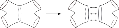
Figure 3: Pants decomposition of a hyperbolic surface.

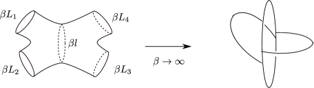
Figure 4: The $\beta\to\infty$ limit.

In this limit, the decomposition in Figure 3 becomes the one in Figure 2. Therefore the decomposition in Figure 2 can be considered as a combinatorial version of the pants decomposition. The combinatorial pairs of pants can be obtained by taking the $\beta\to\infty$ limit of the hyperbolic pairs of pants as in Figure 5. They have different shapes depending on the lengths of the three boundary components.

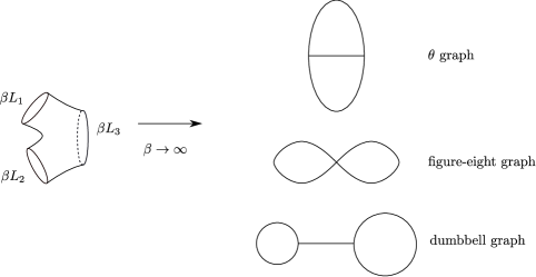
Figure 5: The combinatorial pairs of pants.

Mondello [19, 20] and Do [21] showed that this intuitive picture is true mathematically. Hence we expect that various notions defined for hyperbolic surfaces can also be defined for metric ribbon graphs. In [15], it was shown that the description of the combinatorial moduli space can be given in parallel to that of the moduli space of hyperbolic surfaces, as we will explain in the following.

Let $\mathcal{M}_{g,n}(\mathbf{L})$ denote the moduli space of hyperbolic surfaces of genus $g$ with $n$ boundary components, whose boundary components are geodesics with lengths $\mathbf{L}=(L_{1},\cdots,L_{n})$. Cutting a surface $\Sigma_{g,n,\mathbf{L}}\in\mathcal{M}_{g,n}(\mathbf{L})$ along non-peripheral simple closed geodesics, we can decompose it into $2g-2+n$ pairs of pants with geodesic boundary. There are many choices for such decomposition and here we pick one. The hyperbolic structure of the surface is specified by the lengths of the simple closed geodesics and the way how boundaries of pairs of pants are identified. Therefore $\mathcal{M}_{g,n}(\mathbf{L})$ can be parametrized locally by the Fenchel-Nielsen coordinates $(l_{s};\tau_{s})\ (s=1,\cdots,3g-3+n)$, where $l_{s}$ are the lengths of the simple closed geodesics and $\tau_{s}$ denote the twist parameters which specify how boundaries of different pairs of pants are identified on $\Sigma_{g,n,\mathbf{L}}$. The Fenchel-Nielsen coordinates are global coordinates on the Teichmüller space $\mathcal{T}_{g,n}(\mathbf{L})$, which corresponds to the region $0<l_{s}<\infty,-\infty<\tau_{s}<\infty$. The moduli space $\mathcal{M}_{g,n}(\mathbf{L})$ is given as

$$\mathcal{M}_{g,n}(\mathbf{L})=\mathcal{T}_{g,n}(\mathbf{L})/\mathrm{Mod}_{g,n}\,,$$

where $\mathrm{Mod}_{g,n}$ denotes the boundary label-preserving mapping class group.

For the combinatorial moduli space, one can define the pants decomposition and the Fenchel-Nielsen coordinates in a similar way. Let $G_{g,n,\mathbf{L}}\in\mathcal{M}_{g,n}^{\mathrm{comb}}(\mathbf{L})$ be a metric ribbon graph, whose boundary components are labeled by indices $a=1,\cdots,n$ and have lengths $\mathbf{L}=(L_{1},\cdots,L_{n})$. As mentioned above, one can decompose $G_{g,n,\mathbf{L}}$ into $2g-2+n$ combinatorial pairs of pants. This can be done without resorting to the $\beta\to\infty$ limit of hyperbolic surfaces via the following procedure. Roughly speaking, what we should do is to thicken $G_{g,n,\mathbf{L}}$, cut it along $3g-3+n$ non boundary parallel (also called essential) simple closed curves to get $2g-2+n$ pairs of pants, and shrink them back to metric ribbon graphs (Figure 6). A simple closed curve on thickened $G_{g,n,\mathbf{L}}$ corresponds to a non-backtracking closed curve $\gamma$ on $G_{g,n,\mathbf{L}}$, which travels along its edges. In general, $\gamma$ visits some edges of $G_{g,n,\mathbf{L}}$ multiple number of times (Figure 7). Given such a decomposition, it is easy to write down an equation like (2) for $\delta_{G_{g,n,\mathbf{L}}}$.

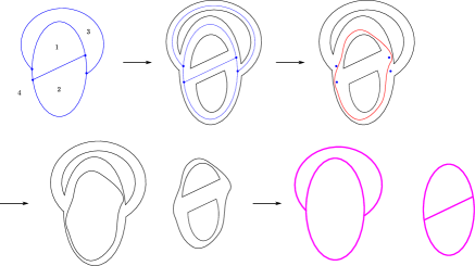
Figure 6: A pants decomposition of a metric ribbon graph. We get two $\theta$ graphs.

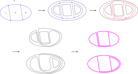
Figure 7: A pants decomposition of a metric ribbon graph. We get two dumbbell graphs.

The above intuitively explained procedure is defined precisely in [15]. What we loosely call “thickened $G_{g,n,\mathbf{L}}$” is given as the geometric realization $\left|G_{g,n,\mathbf{L}}\right|$ of $G_{g,n,\mathbf{L}}$ defined as follows. Given an edge $e$ of $G_{g,n,\mathbf{L}}$, we thicken it by considering $e\times I$, where $I=\left\{y\,|\,-1\leq y\leq 1\right\}$ is a closed interval. We get a rectangle as depicted in Figure 8 on which we have coordinates $(x,y)$ where $x$ is a coordinate on $e$ satisfying $dx=\sqrt{\varphi(z)}dz$ with $\varphi(z)dz^{2}$ being the Strebel differential on $\mathrm{gr}_{\infty}(G_{g,n,\mathbf{L}})$. The rectangle is foliated by leaves given by the curves $x=\text{constant}$. The edge $e$ is identified with the curve $y=0$. At the vertices of $\left|G_{g,n,\mathbf{L}}\right|$ where three edges meet, we glue the thickened edges as illustrated in Figure 8. The gluing rule is defined for other cases in a similar way. Gluing all thickened edges, we get a genus $g$ surface with $n$ boundary components which is denoted by $\left|G_{g,n,\mathbf{L}}\right|$. The construction looks quite like that of Feynman diagrams in Witten’s open string field theory [22]. We have a foliation with isolated singularities on $\left|G_{g,n,\mathbf{L}}\right|$ which is equipped with the transverse measure $\left|dx\right|$, by which we can define the lengths of arcs transverse to the foliation. Such a foliation is called a measured foliation [23, 24, 25].

The surface $\left|G_{g,n,\mathbf{L}}\right|$ can be cut along $3g-3+n$ essential simple closed curves so that we get $2g-2+n$ pairs of pants. By deforming the curves homotopically and changing the foliation if necessary, we can take the curves to be transverse to the foliation. Then each pair of pants inherits the measured foliation which is equivalent to that of $\left|G_{0,3,\mathbf{L}}\right|$ for some $\mathbf{L}=(L_{1},L_{2},L_{3})$. $L_{1},L_{2},L_{3}$ coincide with the combinatorial lengths of the boundary components of the pair of pants, defined through the transverse measure. If we shrink the pairs of pants down to the combinatorial ones, we get a combinatorial pants decomposition of $G_{g,n,\mathbf{L}}$.

Given a pants decomposition, the combinatorial Fenchel-Nielsen coordinates $(l_{s}^{\mathrm{comb}};\tau_{s}^{\mathrm{comb}})\ (s=1,\cdots,3g-3+n)$ are defined by using the measured foliation on $\left|G_{g,n,\mathbf{L}}\right|$. $l_{s}^{\mathrm{comb}}$ coincide with the combinatorial lengths of the closed curves on $\left|G_{g,n,\mathbf{L}}\right|$, along which $\left|G_{g,n,\mathbf{L}}\right|$ is cut. $\tau_{s}$ denote the twist parameters which specify how boundaries of different pairs of pants are identified on $\left|G_{g,n,\mathbf{L}}\right|$. Unlike the Fenchel-Nielsen coordinates for hyperbolic surfaces, for fixed $(l_{1}^{\mathrm{comb}},\cdots,l_{3g-3+n}^{\mathrm{comb}})\in\mathbb{R}_{+}^{3g-3+n}$, some values of $(\tau_{1}^{\mathrm{comb}},\cdots,\tau_{3g-3+n}^{\mathrm{comb}})\in\mathbb{R}^{3g-3+n}$ are not admissible [15]. An example of such a twist is presented in appendix B. However, the non-admissible values of $\tau_{s}$ are of measure zero and the coordinates $(l_{s}^{\mathrm{comb}};\tau_{s}^{\mathrm{comb}})$ with $0<l_{s}<\infty,-\infty<\tau_{s}<\infty$. are almost everywhere global coordinates on the combinatorial version of the Teichmüller space $\mathcal{T}_{g,n}^{\mathrm{comb}}(\mathbf{L})$. The moduli space $\mathcal{M}_{g,n}^{\mathrm{comb}}(\mathbf{L})$ is given as

$$\mathcal{M}_{g,n}^{\mathrm{comb}}(\mathbf{L})=\mathcal{T}_{g,n}^{\mathrm{comb}}(\mathbf{L})/\mathrm{Mod}_{g,n}\,.$$

Hence the combinatorial Fenchel-Nielsen coordinates $(l_{s}^{\mathrm{comb}};\tau_{s}^{\mathrm{comb}})$ can be used as local coordinates on $\mathcal{M}_{g,n}^{\mathrm{comb}}(\mathbf{L})$.

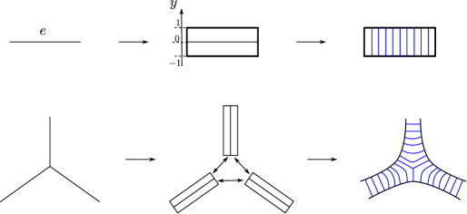
Figure 8: $\left|G_{g,n,\mathbf{L}}\right|$ and the measured foliation.

2.2 The surface states

The expression (1) is rather formal but one can make it tractable by introducing the surface states. As is described in appendix A, given $G_{g,n,\mathbf{L}}\in\mathcal{M}_{g,n}^{\mathrm{comb}}(\mathbf{L})$, we can construct a punctured Riemann surface $\mathrm{gr}_{\infty}(G_{g,n,\mathbf{L}})$ by attaching semi-infinite cylinders $D_{a}$ to the boundary components of $G_{g,n,\mathbf{L}}$. We take the local coordinate $u_{a}$ on $D_{a}$, as explained in appendix A. In this way, from $G_{g,n,\mathbf{L}}$ we obtain a punctured Riemann surface $\mathrm{gr}_{\infty}(G_{g,n,\mathbf{L}})$ with local coordinates $u_{a}$ defined up to phases around the punctures $u_{a}=0$. Let $\mathcal{H}$ denote the state space of the worldsheet theory. We define the surface state $|G_{g,n,\mathbf{L}}\rangle\in\mathcal{H}^{\otimes n}$ associated to the punctured Riemann surface $\mathrm{gr}_{\infty}(G_{g,n,\mathbf{L}})$ with local coordinates $u_{a}$ to satisfy

$${}_{1\cdots n}\langle G_{g,n,\mathbf{L}}|\Psi_{1}\rangle_{1}\cdots|\Psi_{n}\rangle_{n}=\langle\prod_{a=1}^{n}u_{a}^{-1}\circ\mathcal{O}_{\Psi_{a}}(0)\rangle_{\mathrm{gr}_{\infty}(G_{g,n,\mathbf{L}})}\,.$$ (3)

Here $\langle G_{g,n,\mathbf{L}}|$ denotes the BPZ conjugate of $|G_{g,n,\mathbf{L}}\rangle$, $\mathcal{O}_{\Psi_{a}}$ denotes the operator corresponding to the state $|\Psi_{a}\rangle\in\mathcal{H}$ and $\left\langle\cdot\right\rangle_{\Sigma}$ denotes the correlation function of the worldsheet theory on surface $\Sigma$. Since $|G_{g,n,\mathbf{L}}\rangle$ is uniquely determined by the values of $\langle G_{g,n,\mathbf{L}}|\Psi_{1}\rangle\cdots|\Psi_{n}\rangle$, (3) can be regarded as giving a definition of the surface state $|G_{g,n,\mathbf{L}}\rangle$.

The surface state $|G_{g,n,\mathbf{L}}\rangle\in\mathcal{H}^{\otimes n}$ is the state such that

$${}_{1\cdots n}\langle G_{g,n,\mathbf{L}}|X^{(1)}\rangle_{1}\cdots|X^{(n)}\rangle_{n}=\delta_{G_{g,n,\mathbf{L}}}\left[X^{(1)},\cdots,X^{(n)}\right]\,,$$

holds, where $|X\rangle$ denotes the coherent state of $X$. Indeed, $n$ point correlation functions of the worldsheet conformal field theory on $\mathrm{gr}_{\infty}(G_{g,n,\mathbf{L}})$ will be given by

$$\int\left[dX^{(1)}\cdots dX^{(n)}\right]\delta_{G_{g,n,\mathbf{L}}}\left[X^{(1)},\cdots,X^{(n)}\right]\Psi_{1}\left[X^{(1)}\right]\cdots\Psi_{n}\left[X^{(n)}\right]$$

$$\quad={}_{1\cdots n}\langle G_{g,n,\mathbf{L}}|\Psi_{1}\rangle_{1}\cdots|\Psi_{n}\rangle_{n}\,,$$

where $\Psi_{a}\left[X^{(a)}\right]=\langle X^{(a)}|\Psi_{a}\rangle\ (a=1,\cdots,n)$. Taking $|\Psi_{a}\rangle=\mathcal{O}_{\Psi_{a}}(0)|0\rangle$, we obtain (3).

Using the surface state, (2) can be recast in the form

$${}_{1234}\langle G|={}_{125}\langle G_{3}|{}_{634}\langle G_{3}^{\prime}|R_{56}\rangle\,,$$ (4)

where $|R_{aa^{\prime}}\rangle\in\mathcal{H}^{\otimes 2}$ denotes the reflector satisfying

$${}_{a}\langle\phi|R_{aa^{\prime}}\rangle=|\phi\rangle_{a^{\prime}}\,,$$

for any $|\phi\rangle\in\mathcal{H}$. For general $(g,n)$, we have factorization identities of the forms

$${}_{1\cdots n}\langle G_{g,n,\mathbf{L}}| = {}_{1\cdots n_{1}\,-1}\langle G_{g_{1},n_{1}+1,\mathbf{L}_{1}}|\ {}_{0\,n_{1}+1\cdots n}\langle G_{g_{2},n_{2}+1,\mathbf{L}_{2}}|R_{-1\,0}\rangle\,,$$

$${}_{1\cdots n}\langle G_{g,n,\mathbf{L}}| = {}_{1\cdots n\,-1\,0}\langle G_{g-1,n+2,\mathbf{L^{\prime}}}|R_{-1\,0}\rangle\,,$$ (5)

with $g_{1}+g_{2}=g,\,n_{1}+n_{2}=n$.

2.3 Three string vertices

In the string field theory we will construct, $\langle G_{g,n,\mathbf{L}}|$ is expressed in terms of three string vertices using the factorization identities (5). The three string vertex corresponds to a surface state $\langle G_{0,3,\mathbf{L}}|$ for $G_{0,3,\mathbf{L}}\in\mathcal{M}_{0,3}^{\mathrm{comb}}(\mathbf{L})$ with $\mathbf{L}=(L_{1},L_{2},L_{3})$. $\langle G_{0,3,\mathbf{L}}|$ satisfies

$$\langle G_{0,3,\mathbf{L}}|\Psi_{1}\rangle|\Psi_{2}\rangle|\Psi_{3}\rangle=\langle\prod_{k=1}^{3}U_{k}^{-1}\circ\mathcal{O}_{\Psi_{k}}(0)\rangle_{\mathrm{gr}_{\infty}(G_{0,3,\mathbf{L}})}\,,$$ (6)

where $U_{k}\ (k=1,2,3)$ are used for the $u_{a}$ in (3) for later convenience. $\mathrm{gr}_{\infty}(G_{0,3,\mathbf{L}})$ can be expressed by the Riemann sphere $\hat{\mathbb{C}}$ with three punctures. Let $z$ be the global complex coordinate on $\hat{\mathbb{C}}$. We take the punctures to be at $z=z_{k}\ (k=1,2,3)$ with $(z_{1},z_{2},z_{3})=(0,1,\infty)$. Let $\Phi(z)dz^{2}$ be the Strebel differential. It is fixed by the conditions that

$$\Phi(z)dz^{2}\sim\left(-\frac{1}{(2\pi)^{2}}\frac{L_{k}^{2}}{(z-z_{k})^{2}}+\cdots\right)dz^{2}\,,$$

for $z\sim z_{k}$ and $\Phi(z)$ is holomorphic for $z\neq z_{k}$. We get

$$\Phi(z)dz^{2} = -\frac{1}{(2\pi)^{2}}\left[\frac{L_{1}^{2}}{z^{2}}+\frac{L_{2}^{2}}{(z-1)^{2}}+\frac{L_{3}^{2}-L_{1}^{2}-L_{2}^{2}}{z(z-1)}\right]dz^{2}\,,$$ (7)

$$= -\frac{L_{3}^{2}z^{2}+(L_{2}^{2}-L_{1}^{2}-L_{3}^{2})z+L_{1}^{2}}{(2\pi)^{2}z^{2}(z-1)^{2}}dz^{2}\,.$$

It is possible to show that

$$\Phi(w)dw^{2}=\begin{cases}\left.\Phi(z)dz^{2}\right|_{L_{1}\leftrightarrow L_{2}}&\text{ for }w=1-z\\ \left.\Phi(z)dz^{2}\right|_{L_{1}\leftrightarrow L_{3}}&\text{ for }w=\frac{1}{z}\\ \left.\Phi(z)dz^{2}\right|_{L_{2}\leftrightarrow L_{3}}&\text{ for }w=\frac{z}{z-1}\end{cases}\,,$$ (8)

holds.

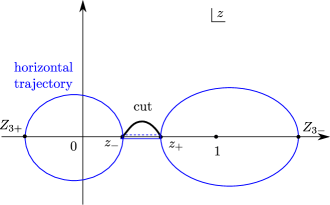
Figure 9: The case $D>0,\ 0<z_{-}<z_{+}<1$.

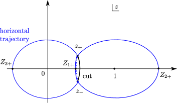
Figure 10: The case $D<0$.

The vertices of the metric ribbon graph $G_{0,3,\mathbf{L}}$ correspond to the solutions of the equation

$$\Phi(z)=0\,.$$ (9)

There are generically two solutions $z=z_{\pm}$ to (9) where

$$z_{\pm}=\frac{L_{1}^{2}-L_{2}^{2}+L_{3}^{2}\pm\sqrt{D}}{2L_{3}^{2}}\,,$$ (10)

with

$$D=-(L_{1}+L_{2}+L_{3})\prod_{k=1}^{3}(L_{1}+L_{2}+L_{3}-2L_{k})\,.$$ (11)

$D<0,\,D=0$ and $D>0$ correspond to $\theta$ graph, figure-eight graph and dumbbell graph depicted in Figure 5, respectively.

Since the state $\langle G_{0,3,\mathbf{L}}|$ is uniquely fixed by the condition (6), we would like to calculate the local coordinate $U_{k}$, which is equal to

$$e^{\pm\frac{2\pi i}{L_{k}}\int^{z}dz^{\prime}\sqrt{\Phi(z^{\prime})}}\,,$$ (12)

up to a phase. The sign in the exponent should be chosen so that $U_{k}=0$ corresponds to $z=z_{k}$. The explicit form of the integral in the exponent is given by

$$\int^{z}dz^{\prime}\sqrt{\Phi(z^{\prime})} = \frac{i}{2\pi}\left[-L_{1}\log\frac{(L_{2}^{2}-L_{1}^{2}-L_{3}^{2})z+2L_{1}^{2}-2L_{1}\sqrt{L_{3}^{2}z^{2}+(L_{2}^{2}-L_{1}^{2}-L_{3}^{2})z+L_{1}^{2}}}{z}\right.$$ (13)

$$\quad\hphantom{\frac{1}{2\pi}}+L_{2}\log\frac{(L_{2}^{2}-L_{1}^{2}+L_{3}^{2})(z-1)+2L_{2}^{2}-2L_{2}\sqrt{L_{3}^{2}z^{2}+(L_{2}^{2}-L_{1}^{2}-L_{3}^{2})z+L_{1}^{2}}}{z-1}$$

$$\quad\hphantom{\frac{1}{2\pi}}+L_{3}\log\left(2L_{3}^{2}z+L_{2}^{2}-L_{1}^{2}-L_{3}^{2}+2L_{3}\sqrt{L_{3}^{2}z^{2}+(L_{2}^{2}-L_{1}^{2}-L_{3}^{2})z+L_{1}^{2}}\right)\left.\vphantom{\frac{(L_{2}^{2}-L_{1}^{2}-L_{3}^{2})z+2L_{1}^{2}-2L_{1}\sqrt{L_{3}^{2}z^{2}+(L_{2}^{2}-L_{1}^{2}-L_{3}^{2})z+L_{1}^{2}}}{z}}\right]\,.$$

We take the cut of the function

$$\sqrt{L_{3}^{2}z^{2}+(L_{2}^{2}-L_{1}^{2}-L_{3}^{2})z+L_{1}^{2}}\,,$$

to be a curve which connects $z_{+}$ to $z_{-}$.

Let us first consider the case $D>0$, which corresponds to either $L_{1}+L_{2}<L_{3}$, $L_{1}+L_{3}<L_{2}$ or $L_{2}+L_{3}<L_{1}$. For $L_{1}+L_{2}<L_{3}$ , $0<z_{-}<z_{+}<1$ holds and the cut can be taken to be the one shown in Figure 9. We obtain

$$\sqrt{L_{3}^{2}z^{2}+(L_{2}^{2}-L_{1}^{2}-L_{3}^{2})z+L_{1}^{2}}\sim\begin{cases}-L_{1}&z\sim 0\\ L_{2}&z\sim 1\\ L_{3}z&z\sim\infty\end{cases}\,,$$ (14)

and

$$\int^{z}dz^{\prime}\sqrt{\Phi(z^{\prime})}\sim\begin{cases}\frac{i}{2\pi}L_{1}\log z&z\sim 0\\ \frac{i}{2\pi}L_{2}\log(z-1)&z\sim 1\\ \frac{i}{2\pi}L_{3}\log z&z\sim\infty\end{cases}\,.$$ (15)

Therefore we should take

$$U_{1} = e^{-\frac{2\pi i}{L_{1}}\int_{Z_{1}}^{z}dz^{\prime}\sqrt{\Phi(z^{\prime})}}\,,$$

$$U_{2} = e^{-\frac{2\pi i}{L_{2}}\int_{Z_{2}}^{z}dz^{\prime}\sqrt{\Phi(z^{\prime})}}\,,$$

$$U_{3} = e^{\frac{2\pi i}{L_{3}}\int_{Z_{3}}^{z}dz^{\prime}\sqrt{\Phi(z^{\prime})}}\,.$$ (16)

Here $Z_{1},Z_{2},Z_{3}$ are chosen to be $Z_{3+}$ or $z_{-}$, $z_{+}$ or $Z_{3-}$, $Z_{3-}$ or $Z_{3+}$ in Figure 9 respectively. Other cases can be dealt with in the same way or one can use (8) to get the formulas for $U_{k}$.

Let us turn to the case $D<0$. Taking the cut shown in Figure 10, we get (16) with $Z_{1},Z_{2},Z_{3}$ chosen to be $Z_{3+}$ or $Z_{1+}$, $Z_{1+}$ or $Z_{2+}$, $Z_{2+}$ or $Z_{3+}$ in the figure respectively. $D=0$ is realized as a limiting case.

2.4 $b$ ghost insertions

We would like to construct a theory in which the amplitudes are described by the contact interactions of strings represented by the critical graphs. For this purpose, we utilize the combinatorial moduli space $\mathcal{M}_{g,n}^{\mathrm{comb}}(\mathbf{L})$ to describe the moduli space. The amplitudes will be expressed by integrals of the form

$$\int_{\mathcal{M}_{g,n}^{\mathrm{comb}}(\mathbf{L})}\langle B_{6g-6+2n}\prod_{a=1}^{n}u_{a}^{-1}\circ\mathcal{O}_{\Psi_{a}}(0)\rangle_{\mathrm{gr}_{\infty}(G_{g,n,\mathbf{L}})}\,,$$

where $\Psi_{a}$ are the external states. $B_{6g-6+2n}$ on the right hand side is given by

$$B_{6g-6+2n}=\prod_{s=1}^{3g-3+n}\left[b(\partial_{l_{s}^{\mathrm{comb}}})b(\partial_{\tau_{s}^{\mathrm{comb}}})\right]\bigwedge_{s=1}^{3g-3+n}\left[dl_{s}^{\mathrm{comb}}\wedge d\tau_{s}^{\mathrm{comb}}\right]\,.$$ (17)

Here $(l_{s}^{\mathrm{comb}};\tau_{s}^{\mathrm{comb}})\ (s=1,\cdots,3g-3+n)$ are the combinatorial Fenchel-Nielsen coordinates on $\mathcal{M}_{g,n}^{\mathrm{comb}}(\mathbf{L})$ corresponding to a pants decomposition of $G_{g,n,\mathbf{L}}$. $b(\partial_{l_{s}^{\mathrm{comb}}})$ and $b(\partial_{\tau_{s}^{\mathrm{comb}}})$ are the $b$ ghost insertions corresponding to the tangent vectors $\partial_{l_{s}^{\mathrm{comb}}}$ and $\partial_{\tau_{s}^{\mathrm{comb}}}$ on $\mathcal{M}_{g,n}^{\mathrm{comb}}(\mathbf{L})$ respectively.

In general, the $b$ ghost insertions are defined as follows [7, 26, 27, 28, 29]. Cutting the worldsheet along circles $\left\{C_{A}\right\}$, we decompose it into coordinate patches. We fix the orientation of $C_{A}$ so that $\sigma_{A}$ and $\sigma_{A}^{\prime}$ are the complex coordinates on the left and the right of $C_{A}$ respectively. These two coordinates are related by a transition function as

$$\sigma_{A}=F_{A}(\sigma_{A}^{\prime})\,,$$

where $F_{A}$ is a holomorphic function in a neighborhood of $C_{A}$. Let $x_{t}\ (t=1,\cdots,6g-6+2n)$ be coordinates on the moduli space. Then the $b$ ghost insertion corresponding to the tangent vector $\partial_{x_{t}}$ is given by

$$b(\partial_{x_{t}})=\sum_{A}\left[\oint_{C_{\beta}}\frac{d\sigma_{A}}{2\pi i}\frac{\partial F_{A}}{\partial x_{t}}b(\sigma_{A})+\text{c.c.}\right]\,,$$ (18)

where c.c. denotes the antiholomorphic contribution.

In our case, we decompose $\mathrm{gr}_{\infty}(G_{g,n,\mathbf{L}})$ into coordinate patches in the following way. Let us assume that $G_{g,n,\mathbf{L}}$ is a trivalent graph. For $\epsilon>0$, we define $\tilde{D}_{a}^{\epsilon}\subset D_{a}\ (a=1,\cdots,n)$ to be the region given by $\left|u_{a}\right|\leq e^{-\frac{2\pi}{L_{a}}\epsilon}$. It is easy to see that $\mathrm{gr}_{\infty}(G_{g,n,\mathbf{L}})\backslash\cup_{a}\tilde{D}_{a}^{\epsilon}$ is homeomorphic to $\left|G_{g,n,\mathbf{L}}\right|$. Indeed $\mathrm{gr}_{\infty}(G_{g,n,\mathbf{L}})\backslash\cup_{a}\tilde{D}_{a}^{\epsilon}$ is made from rectangular neighborhoods of edges of $G_{g,n,\mathbf{L}}$ on which one can define coordinates $(x,y)\ (-1\leq y\leq 1)$ such that

$$\epsilon y+ix=\int_{z_{0}}^{z}dz^{\prime}\sqrt{\varphi(z^{\prime})}\,,$$ (19)

where $z$ denotes a local coordinate on $\mathrm{gr}_{\infty}(G_{g,n,\mathbf{L}})\backslash\cup_{a}\tilde{D}_{a}^{\epsilon}$ and $z_{0}$ corresponds to a point on the edge. At the vertices the rectangles are glued together as in Figure 8. With the transverse measure $\left|dx\right|$, one can define a measured foliation on $\mathrm{gr}_{\infty}(G_{g,n,\mathbf{L}})\backslash\cup_{a}\tilde{D}_{a}^{\epsilon}$ in the same way as in the case of $\left|G_{g,n,\mathbf{L}}\right|$. Therefore we may identify $\mathrm{gr}_{\infty}(G_{g,n,\mathbf{L}})\backslash\cup_{a}\tilde{D}_{a}^{\epsilon}$ with $\left|G_{g,n,\mathbf{L}}\right|$ using the homeomorphism.

The pants decomposition of $G_{g,n,\mathbf{L}}$ corresponding to the Fenchel-Nielsen coordinates is obtained by cutting $\left|G_{g,n,\mathbf{L}}\right|$ along simple closed curves transverse to the foliation. By cutting $\mathrm{gr}_{\infty}(G_{g,n,\mathbf{L}})\backslash\cup_{a}\tilde{D}_{a}^{\epsilon}$ along these curves, we can decompose it into $2g-2+n$ pairs of pants. Let $S_{i}^{\epsilon}\ (i=1,\cdots,2g-2+n)$ denote the closure of these pairs of pants. $\mathrm{gr}_{\infty}(G_{g,n,\mathbf{L}})$ is decomposed into $S_{i}^{\epsilon}$ and $\tilde{D}_{a}^{\epsilon}$. The decomposition can be obtained by cutting $\mathrm{gr}_{\infty}(G_{g,n,\mathbf{L}})$ along $3g-3+2n$ circles.

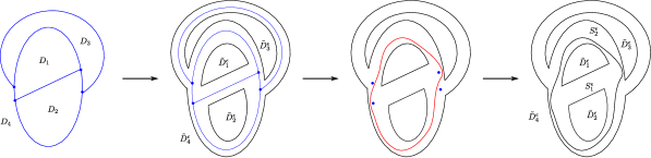
Figure 11: Coordinate patches on $\mathrm{gr}_{\infty}(G_{g,n,\mathbf{L}})$.

If the measured foliation on $S_{i}^{\epsilon}$ is equivalent to that on $\left|G_{0,3,(L_{1},L_{2},L_{3})}\right|$, one can construct a conformal map from $S_{i}^{\epsilon}$ to $\mathrm{gr}_{\infty}(G_{0,3,(L_{1},L_{2},L_{3})})$ in the following way. $\mathrm{gr}_{\infty}(G_{0,3,(L_{1},L_{2},L_{3})})$ can be expressed by the Riemann sphere $\hat{\mathbb{C}}$ with three punctures. Let $z_{i}$ be the the global complex coordinate on the Riemann sphere $\hat{\mathbb{C}}$ so that the Strebel differential on $\mathrm{gr}_{\infty}(G_{0,3,(L_{1},L_{2},L_{3})})$ is given by

$$\Phi(z_{i})dz_{i}^{2}\,,$$

where $\Phi$ is defined in (7). Then we consider a conformal map from $S_{i}^{\epsilon}$ to $\mathrm{gr}_{\infty}(G_{0,3,(L_{1},L_{2},L_{3})})$ such that the two zeros of $\varphi(z)dz^{2}$ in $S_{i}^{\epsilon}$ are mapped to the zeros of $\Phi(z_{i})dz_{i}^{2}$ and

$$\sqrt{\varphi(z)}dz=\sqrt{\Phi(z_{i})}dz_{i}\,,$$ (20)

is satisfied. The map $z_{i}(z)$ is obtained by solving (20) around the zeros of $\varphi(z)dz^{2}$ and analytically continuing it to other regions in $S_{i}^{\epsilon}$. (20) implies that the rectangular neighborhoods of edges of $G_{g,n,\mathbf{L}}$ are mapped to those of edges of $G_{0,3,(L_{1},L_{2},L_{3})}$. As can be seen from Figure 12, the images of the neighborhoods cover $\mathrm{gr}_{\infty}(G_{0,3,(L_{1},L_{2},L_{3})})\backslash\cup_{k=1}^{3}\tilde{D}_{k}^{\epsilon}$ and $S_{i}^{\epsilon}$ is conformally equivalent to a region in the $z_{i}$ plane.

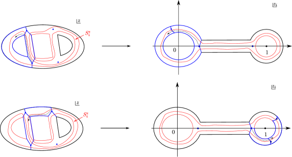
Figure 12: The analytic continuation of $z_{i}(z)$. The rectangular neighborhoods are depicted as hexagons.

Hence $z_{i}$ provides a local coordinate on $S_{i}^{\epsilon}$. $u_{a}$ can be used as a local coordinate on $\tilde{D}_{a}^{\epsilon}$. If $S_{i}^{\epsilon}\cap\tilde{D}_{a}^{\epsilon}=\partial\tilde{D}_{a}^{\epsilon}$, $z_{i}$ and $u_{a}$ are related by

$$z_{i}=U_{k}^{-1}(u_{a})\,,$$ (21)

for some $k\ (k=1,2,3)$ in a neighborhood of $\partial\tilde{D}_{a}^{\epsilon}$. In the same way, we can see that if $S_{i}^{\epsilon}\cap S_{j}^{\epsilon}=\mathrm{C}_{ij}^{\epsilon}$, $z_{i}$ and $z_{j}$ are related by

$$z_{i}=U_{k}^{-1}\left(\frac{e^{i\theta_{ij}}}{U_{k^{\prime}}(z_{j})}\right)\,,$$ (22)

for some $k,k^{\prime}$. Here $\theta_{ij}$ is the twist angle.

Substituting (21) and (22) into (18), we obtain $b(\partial_{l_{s}^{\mathrm{comb}}})$ and $b(\partial_{\tau_{s}^{\mathrm{comb}}})$. $l_{s}^{\mathrm{comb}}$ should be the combinatorial length of $\mathrm{C}_{ij}^{\epsilon}$ for some $i,j$. Hence $b(\partial_{l_{s}^{\mathrm{comb}}})$ can be given by

$$b(\partial_{l_{s}^{\mathrm{comb}}})=b_{S_{i}^{\epsilon}}(\partial_{l_{s}^{\mathrm{comb}}})+b_{S_{j}^{\epsilon}}(\partial_{l_{s}^{\mathrm{comb}}})\,,$$

$$b_{S_{i}^{\epsilon}}(\partial_{l_{s}^{\mathrm{comb}}})=-\oint_{\partial S_{i}^{\epsilon}}\frac{dz_{i}}{2\pi i}\frac{\partial U_{k}(z_{i})}{\partial l_{s}^{\mathrm{comb}}}\left(\frac{\partial U_{k}(z_{i})}{\partial z_{i}}\right)^{-1}b(z_{i})+\text{c.c.}\,,$$

$$b_{S_{j}^{\epsilon}}(\partial_{l_{s}^{\mathrm{comb}}})=-\oint_{\partial S_{j}^{\epsilon}}\frac{dz_{j}}{2\pi i}\frac{\partial U_{k}(z_{j})}{\partial l_{s}^{\mathrm{comb}}}\left(\frac{\partial U_{k}(z_{j})}{\partial z_{j}}\right)^{-1}b(z_{j})+\text{c.c.}\,.$$ (23)

Here $k\ (k=1,2,3)$ for $U_{k}$ in each term is chosen so that $U_{k}$ gives a good coordinate on the relevant component of the boundary. With the choice of $Z_{k}$ in (16), $\partial_{\tau_{s}^{\mathrm{comb}}}=\frac{1}{l_{s}^{\mathrm{comb}}}\partial_{\theta_{ij}}$ and we have

$$b(\partial_{\tau_{s}^{\mathrm{comb}}})=-\frac{2\pi}{l_{s}}\left[\oint_{\mathrm{C}_{ij}^{\epsilon}}\frac{dz_{i}}{2\pi i}iU_{k}(z_{i})\left(\frac{\partial U_{k}(z_{i})}{\partial z_{i}}\right)^{-1}b(z_{i})+\text{c.c.}\right]\,,$$ (24)

where $k$ for $U_{k}$ is chosen so that $U_{k}(z_{i})$ is a good coordinate on $\mathrm{C}_{ij}^{\epsilon}$. The contours run along $\mathrm{C}_{ij}^{\epsilon}$ so that $S_{j}^{\epsilon}$ lies to its left.

In the same way, if $S_{i}^{\epsilon}\cap\tilde{D}_{a}^{\epsilon}=\partial\tilde{D}_{a}^{\epsilon}$, we define

$$b_{S_{i}^{\epsilon}}(\partial_{L_{a}})=-\oint_{\partial S_{i}^{\epsilon}}\frac{dz_{i}}{2\pi i}\frac{\partial U_{k}(z_{i})}{\partial L_{a}}\left(\frac{\partial U_{k}(z_{i})}{\partial z_{i}}\right)^{-1}b(z_{i})+\text{c.c.}\,,$$ (25)

which play important roles in the following. All these formulas look quite similar to those in the hyperbolic case [11].

Thus we have constructed $b$ ghost insertions assuming that $G_{g,n,\mathbf{L}}$ is a trivalent graph. When $G_{g,n,\mathbf{L}}$ is not trivalent, it is not possible to define the coordinate patches $S_{i}^{\epsilon}$ and $\tilde{D}_{a}^{\epsilon}$. However, nontrivalent graphs can be identified as limits of trivalent graphs as lengths of some of the edges go to $0$. Therefore we define $b$ ghost insertions for a nontrivalent graph by Eqs. (23), (24) and (25) in such a limit. For trivalent graphs, these $b$ ghost insertions can be shown to be equal to those using the Schiffer variation [7], for example, by deforming the contours. Since those $b$ ghost insertions are well-defined for nontrivalent graphs, they are well-defined in the limit.

For later use, we will show that (23), (24) and (25) can be expressed in terms of quantities defined on the ribbon graph. We can do so by taking the $\epsilon\to 0$ limit using the fact that the $b$ ghost insertions do not depend on $\epsilon$. On the $z_{i}$ plane, for $l_{s}^{\mathrm{comb}}=L_{k^{\prime}}$, $b(\partial_{\tau_{s}^{\mathrm{comb}}})$ is recast into

$$\pm\oint_{\partial\tilde{D}_{k^{\prime}}^{\epsilon}}\frac{dz_{i}}{2\pi i}\frac{1}{\sqrt{\Phi(z_{i})}}b(z_{i})+\text{c.c.}\,,$$

using (16), and it can be shown to be equal to

$$\lim_{\epsilon\to 0}b(\partial_{\tau_{s}^{\mathrm{comb}}})=\pm\oint_{\partial D_{k^{\prime}}}\frac{dz_{i}}{2\pi i}\frac{1}{\sqrt{\Phi(z_{i})}}b(z_{i})+\text{c.c.}\,,$$ (26)

by a contour deformation. The right hand side of (26) is given in terms of quantities defined on the ribbon graph. In the same way, $b_{S_{i}^{\epsilon}}(\partial_{l_{s}^{\mathrm{comb}}})$ can be transformed into

$$-\sum_{k=1}^{3}\oint_{\partial\tilde{D}_{k}^{\epsilon}}\frac{dz_{i}}{2\pi i}\frac{\partial}{\partial L_{k^{\prime}}}\left(\frac{1}{L_{k}}\int_{Z_{k}}^{z_{i}}dz^{\prime}\sqrt{\Phi(z^{\prime})}\right)\frac{L_{k}}{\sqrt{\Phi(z_{i})}}b(z_{i})+\text{c.c.}$$

$$\quad=-\sum_{k=1}^{3}\oint_{\partial\tilde{D}_{k}^{\epsilon}}\frac{dz_{i}}{2\pi i}\frac{\partial}{\partial L_{k^{\prime}}}\left(\int_{Z_{k}}^{z_{i}}dz^{\prime}\sqrt{\Phi(z^{\prime})}\right)\frac{1}{\sqrt{\Phi(z_{i})}}b(z_{i})$$

$$\hphantom{\quad=}+\frac{1}{L_{k^{\prime}}}\oint_{\partial\tilde{D}_{k^{\prime}}^{\epsilon}}\frac{dz_{i}}{2\pi i}\frac{1}{\sqrt{\Phi(z_{i})}}b(z_{i})\int_{Z_{k^{\prime}}}^{z_{i}}dz^{\prime}\sqrt{\Phi(z^{\prime})}$$

$$\hphantom{\quad=}+\text{c.c.}\,.$$

In this case, the function $\frac{\partial}{\partial L_{k^{\prime}}}\left(\int_{Z_{k}}^{z_{i}}dz^{\prime}\sqrt{\Phi(z^{\prime})}\right)\frac{1}{\sqrt{\Phi(z_{i})}}$ in the integrand develops poles at $z_{i}=z_{\pm}$. This function can be expressed as

$$\frac{\partial}{\partial L_{k^{\prime}}}\left(\int_{Z_{k}}^{z_{i}}dz^{\prime}\sqrt{\Phi(z^{\prime})}\right)\frac{1}{\sqrt{\Phi(z_{i})}}$$

$$\quad=\frac{\partial z_{+}}{\partial L_{k^{\prime}}}\frac{a_{+}}{z_{i}-z_{+}}+\frac{\partial z_{-}}{\partial L_{k^{\prime}}}\frac{a_{-}}{z_{i}-z_{-}}+R_{k^{\prime}}(z_{i})\,,$$

where $a_{\pm}$ are constants and $R_{k^{\prime}}(z_{i})$ is a function which does not have poles at $z_{i}=z_{\pm}$. Using this formula, we can show that $b_{S_{i}^{\epsilon}}(\partial_{l_{s}^{\mathrm{comb}}})$ is equal to

$$b_{S_{i}^{0}}(\partial_{l_{s}^{\mathrm{comb}}}) \equiv \lim_{\epsilon\to 0}b_{S_{a}^{\epsilon}}(\partial_{l_{s}^{\mathrm{comb}}})$$ (27)

$$= a_{+}\frac{\partial z_{+}}{\partial L_{k^{\prime}}}b(z_{+})+a_{-}\frac{\partial z_{-}}{\partial L_{k^{\prime}}}b(z_{-})$$

$$-\sum_{k=1}^{3}\oint_{\partial D_{k}}\frac{dz_{i}}{2\pi i}R_{k^{\prime}}(z_{i})b(z_{i})$$

$$+\frac{1}{L_{k^{\prime}}}\oint_{\partial D_{k^{\prime}}}\frac{dz_{i}}{2\pi i}\frac{1}{\sqrt{\Phi(z_{i})}}b(z_{i})\int_{Z_{k^{\prime}}}^{z_{i}}dz^{\prime}\sqrt{\Phi(z^{\prime})}$$

$$+\text{c.c.}\,.$$

The right hand side of this equation consists of quantities defined on the critical graph on the $z_{i}$ plane. Using $\eqref{eq:rootphi}$, we can express the right hand sides of (26) and (27) in terms of quantities defined on $G_{g,n,\mathbf{L}}$ as long as $G_{g,n,\mathbf{L}}$ is trivalent. $b_{S_{i}^{0}}(\partial_{L_{a}})$ is defined in the same way and can be shown to be equal to $b_{S_{i}^{\epsilon}}(\partial_{L_{a}})$.

2.5 The off-shell amplitudes

Since $b(\partial_{l_{s}^{\mathrm{comb}}})$ and $b(\partial_{\tau_{s}^{\mathrm{comb}}})$ can be expressed in terms of quantities defined on $G_{g,n,\mathbf{L}}$, one can represent $B_{6g-6+2n}$ in (17) as an operator acting on the surface state $\langle G_{g,n,\mathbf{L}}|$. Let $\mathcal{H}_{0}$ denote the subspace of $\mathcal{H}$, which consists of the states $|\Psi\rangle$ satisfying

$$b_{0}^{-}|\Psi\rangle=(L_{0}-\bar{L}_{0})|\Psi\rangle=0\,,$$ (28)

where $b_{0}^{\pm}\equiv b_{0}\pm\bar{b}_{0}$. In our setup, the external lines for the off-shell amplitudes are labeled by a state in $\mathcal{H}_{0}$ and the length of the string. We define $g$ loop $n$ string amplitudes for $g\geq 0,\ n\geq 1,\ 2g-2+n>0$ to be

$$A_{g,n}\left((|\Psi_{1}\rangle,L_{1}),\cdots,(|\Psi_{n}\rangle,L_{n})\right)=2^{-\delta_{g,1}\delta_{n,1}}(2\pi i)^{-3g+3-n}\int_{\mathcal{M}_{g,n}^{\mathrm{comb}}(\mathbf{L})}\langle G_{g,n,\mathbf{L}}|B_{6g-6+2n}|\Psi_{1}\rangle\cdots|\Psi_{n}\rangle\,,$$ (29)

for $|\Psi_{a}\rangle\in\mathcal{H}_{0}\ (a=1,\cdots,n)$. The factor $2^{-\delta_{g,1}\delta_{n,1}}$ is due to the $\mathbb{Z}_{2}$ symmetry possessed by $G_{1,1,L}$. Since $\mathcal{M}_{g,n}^{\mathrm{comb}}(\mathbf{L})$ is homeomorphic to the moduli space $\mathcal{M}_{g,n}$ of punctured Riemann surfaces $\mathrm{gr}_{\infty}(G_{g,n,\mathbf{L}})$, these amplitudes coincide with the conventional amplitudes when $|\Psi_{a}\rangle$ are on-shell physical states.

In the following, we will manipulate the expression (29) of the amplitudes and derive identities satisfied by them. Since the moduli space $\mathcal{M}_{g,n}^{\mathrm{comb}}(\mathbf{L})$ is noncompact, the amplitudes may suffer from divergences coming from the boundary. What we would like to do is to construct a formalism using which we obtain the expression on the right hand side of (29), and discuss the behavior at the boundary later. In order to proceed, we here assume that there exists a good regularization such that the regularized integrands of the amplitudes go to zero rapidly at the boundary of moduli space. In many cases, the amplitudes may be divergent when the regularization is removed.

3 A recursion relation for the off-shell amplitudes

In calculating the amplitudes (29), $\mathcal{M}_{g,n}^{\mathrm{comb}}(\mathbf{L})$ should be realized as a fundamental domain of $\mathrm{Mod}_{g,n}$ in $\mathcal{T}_{g,n}^{\mathrm{comb}}(\mathbf{L})$ but there is no concrete description of it for general $(g,n)$. In calculations of the volumes $V_{g,n}(\mathbf{L})$ of the moduli spaces $\mathcal{M}_{g,n}(\mathbf{L})$ for hyperbolic surfaces, a similar problem was overcome by Mirzakhani’s integration scheme [12, 13]. Mirzakhani used McShane identity [30] and its generalization (Mirzakhani-McShane identity) to unfold the integrals over $\mathcal{M}_{g,n}(\mathbf{L})$ and make the calculation possible. By doing so, she derived a recursion relation satisfied by $V_{g,n}(\mathbf{L})$.

There exists a generalization of Mirzakhani-McShane identity [14, 15] for combinatorial moduli space $\mathcal{M}_{g,n}^{\mathrm{comb}}(\mathbf{L})$, which can be used to unfold integrals over $\mathcal{M}_{g,n}^{\mathrm{comb}}(\mathbf{L})$. Applying this method to the integral on the right hand side of (29), it is possible to derive a recursion relation satisfied by the off-shell amplitudes.

3.1 Mirzakhani-McShane identity for combinatorial moduli space

Given $G_{g,n,\mathbf{L}}\in\mathcal{M}_{g,n}^{\mathrm{comb}}(\mathbf{L})$, let $\beta_{1},\cdots,\beta_{n}$ be the boundary components of $\left|G_{g,n,\mathbf{L}}\right|$ such that the combinatorial lengths of $\beta_{1},\cdots,\beta_{n}$ are $L_{1},\cdots,L_{n}$ respectively. The Mirzakhani-McShane identity for combinatorial moduli space is given by [15, 14]

$$1=\sum_{a=2}^{n}\sum_{\gamma\in\mathscr{C}_{a}}\mathsf{B}(L_{1},L_{a},l_{\gamma})+\frac{1}{2}\sum_{\left(\gamma,\delta\right)\in\mathscr{C}_{1}}\mathsf{C}(L_{1},l_{\gamma},l_{\delta})\,,$$ (30)

for $3g-3+n>0,\ (g,n)\neq(1,1)$ and

$$1=\sum_{\gamma\in\mathscr{C}^{\mathrm{T}}}\mathsf{C}(L_{1},l_{\gamma},l_{\gamma})\,,$$ (31)

for $(g,n)=(1,1)$. Here

$$\mathscr{C}_{a} \equiv \left\{\begin{array}[]{l}\text{the set of homotopy classes of essential simple closed curves }\gamma\text{ on }\text{$\left|G_{g,n,\mathbf{L}}\right|$}\\ \text{which bound a pair of pants together with the bondary components }\beta_{1}\text{ and }\beta_{a}\end{array}\right\}\,,$$

$$\mathscr{C}_{1} \equiv \left\{\begin{array}[]{l}\text{the set of ordered pairs of homotopy classes of essential simple closed curves }\left(\gamma,\delta\right)\\ \text{on }\text{$\left|G_{g,n,\mathbf{L}}\right|$}\text{ which bound a pair of pants together with the bondary component }\beta_{1}\end{array}\right\}\,,$$

$$\mathscr{C}^{\mathrm{T}} \equiv \left\{\begin{array}[]{l}\text{the set of homotopy classes of essential simple closed curves }\gamma\text{ on }\text{$\left|G_{1,1,L_{1}}\right|$}\end{array}\right\}\,,$$

$l_{\gamma}$ denotes the combinatorial length of $\gamma$ and

$$\mathsf{B}(L_{1},L_{2},L_{3}) = \frac{1}{2L_{1}}\left(\left[L_{1}-L_{2}-L_{3}\right]_{+}-\left[-L_{1}+L_{2}-L_{3}\right]_{+}+\left[L_{1}+L_{2}-L_{3}\right]_{+}\right)$$

$$= \begin{cases}0&L_{1}+L_{2}\leq L_{3}\\ \frac{1}{2L_{1}}\left(L_{1}+L_{2}-L_{3}\right)&\left|L_{1}-L_{2}\right|<L_{3}<L_{1}+L_{2}\\ 1&L_{3}\leq L_{2}-L_{1}\\ \frac{1}{L_{1}}(L_{1}-L_{3})&L_{3}\leq L_{1}-L_{2}\end{cases}\,,$$

$$\mathsf{C}(L_{1},L_{2},L_{3}) = \frac{1}{L_{1}}\left[L_{1}-L_{2}-L_{3}\right]_{+}$$ (35)

$$= \begin{cases}0&L_{1}\leq L_{2}+L_{3}\\ \frac{1}{L_{1}}(L_{1}-L_{2}-L_{3})&L_{2}+L_{3}<L_{1}\end{cases}\,,$$

with $\left[x\right]_{+}=\max\left\{x,0\right\}$. Unlike the hyperbolic case, only a finite number of terms on the right hand sides of (30) and (31) are nonzero because of the definitions of $\mathsf{B}$ and $\mathsf{C}$.

3.2 A recursion relation for the off-shell amplitudes

A recursion relation for the off-shell amplitudes can be derived by following the same procedure as in [11]. Let us first introduce a basis of the state space of the worldsheet theory. We define $\mathcal{H}_{0}^{c}$ to be the subspace of $\mathcal{H}$ which consists of the states $|\Psi\rangle$ satisfying

$$c_{0}^{-}|\Psi\rangle=(L_{0}-\bar{L}_{0})|\Psi\rangle=0\,,$$

with $c_{0}^{\pm}=c_{0}\pm\bar{c}_{0}$. We choose the bases $\{|\varphi_{i}\rangle\}$ and $\{|\varphi_{i}^{c}\rangle\}$ of $\mathcal{H}_{0}$ and $\mathcal{H}_{0}^{c}$ respectively so that

$$\langle\varphi_{i}^{c}|\varphi_{j}\rangle = \delta_{ij}\,,$$

$$\langle\varphi_{j}|\varphi_{i}^{c}\rangle = (-1)^{\left|\varphi_{i}\right|}\delta_{ij}\,,$$

$$\sum_{i}|\varphi_{i}\rangle\langle\varphi_{i}^{c}| = \frac{1}{2}b_{0}^{-}c_{0}^{-}P\equiv P_{+}\,,$$

$$\sum_{i}|\varphi_{i}^{c}\rangle\langle\varphi_{i}|(-1)^{\left|\varphi_{i}\right|} = \frac{1}{2}c_{0}^{-}b_{0}^{-}P\equiv P_{-}\,,$$

$$P^{(1)}|R_{12}\rangle = P^{(2)}|R_{12}\rangle=\sum_{i}\left[|\varphi_{i}\rangle_{1}|\varphi_{i}^{c}\rangle_{2}+|\varphi_{i}^{c}\rangle_{1}|\varphi_{i}\rangle_{2}(-1)^{\left|\varphi_{i}\right|}\right]\,,$$ (36)

hold. Here

$$P=\int_{0}^{2\pi}\frac{d\theta}{2\pi}e^{i\theta(L_{0}-\bar{L}_{0})}\,.$$

In order to derive a recursion relation, it is convenient to define the following amplitudes:

$$A_{g,n}^{I_{1}\cdots I_{n}}\equiv 2^{-\delta_{g,1}\delta_{n,1}}(2\pi i)^{-3g+3-n}\int_{\mathcal{M}_{g,n}^{\mathrm{comb}}(\mathbf{L})}\langle G_{g,n,\mathbf{L}}|B_{6g-6+2n}B_{\alpha_{1}}^{1}\cdots B_{\alpha_{n}}^{n}|\varphi_{i_{1}}^{\alpha_{1}}\rangle\cdots|\varphi_{i_{n}}^{\alpha_{n}}\rangle\,.$$ (37)

Here the external lines are labeled by $I_{a}=(i_{a},\alpha_{a},L_{a})\ (a=1,\cdots,n)$. The indices $\alpha_{a}$ take values $\pm$ and

$$|\varphi_{i_{a}}^{\alpha_{a}}\rangle=\begin{cases}|\varphi_{i_{a}}\rangle&\alpha_{a}=+\\ |\varphi_{i_{a}}^{c}\rangle&\alpha_{a}=-\end{cases}\,.$$

$B_{\alpha_{a}}^{a}$is given by

$$B_{\alpha_{a}}^{a}\equiv\begin{cases}1&\alpha_{a}=+\\ b_{0}^{-(a)}b_{S_{a}^{0}}(\partial_{L_{a}})&\alpha_{a}=-\end{cases}\,.$$ (38)

Here we define $S_{a}^{\epsilon}$ to be the pair of pants one of whose boundary component coincides with $\partial\tilde{D}_{a}^{\epsilon}$ in a pants decomposition of $\mathrm{gr}_{\infty}(G_{g,n,\mathbf{L}})\backslash\cup_{a}\tilde{D}_{a}^{\epsilon}$. $b_{S_{a}^{\epsilon}}(\partial_{L_{a}})$ depends on the choice of the pants decomposition, because it corresponds to the variation $L_{a}\to L_{a}+\varepsilon$ with the Fenchel-Nielsen coordinates $l_{s}^{\mathrm{comb}},\tau_{s}^{\mathrm{comb}}$ fixed. However, $b_{S_{a}^{\epsilon}}(\partial_{L_{a}})B_{6g-6+2n}$ does not depend on the choice and the amplitudes in (37) are well-defined.

Now we would like to derive a recursion relation for $A_{g,n}^{I_{1}\cdots I_{n}}$. In order to do so, let us multiply (30) by

$$(2\pi i)^{-3g+3-n}\langle G_{g,n,\mathbf{L}}|B_{6g-6+2n}B_{\alpha_{1}}^{1}\cdots B_{\alpha_{n}}^{n}|\varphi_{i_{1}}^{\alpha_{1}}\rangle\cdots|\varphi_{i_{n}}^{\alpha_{n}}\rangle\,,$$

and integrate over $\mathcal{M}_{g,n}^{\mathrm{comb}}(\mathbf{L})$. We obtain

$$(2\pi i)^{-3g+3-n}\int_{\mathcal{M}_{g,n}^{\mathrm{comb}}(\mathbf{L})}\langle G_{g,n,\mathbf{L}}|B_{6g-6+2n}B_{\alpha_{1}}^{1}\cdots B_{\alpha_{n}}^{n}|\varphi_{i_{1}}^{\alpha_{1}}\rangle\cdots|\varphi_{i_{n}}^{\alpha_{n}}\rangle$$

$$\quad=\sum_{a=2}^{n}\sum_{\gamma\in\mathscr{C}_{a}}\int_{\mathcal{M}_{g,n}^{\mathrm{comb}}(\mathbf{L})}\mathsf{B}(L_{1},L_{a},l_{\gamma})(2\pi i)^{-3g+3-n}\langle G_{g,n,\mathbf{L}}|B_{6g-6+2n}B_{\alpha_{1}}^{1}\cdots B_{\alpha_{n}}^{n}|\varphi_{i_{1}}^{\alpha_{1}}\rangle\cdots|\varphi_{i_{n}}^{\alpha_{n}}\rangle$$

$$\hphantom{\quad=}+\frac{1}{2}\sum_{\left(\gamma,\delta\right)\in\mathscr{C}_{1}}\int_{\mathcal{M}_{g,n}^{\mathrm{comb}}(\mathbf{L})}\mathsf{C}(L_{1},l_{\gamma},l_{\delta})(2\pi i)^{-3g+3-n}\langle G_{g,n,\mathbf{L}}|B_{6g-6+2n}B_{\alpha_{1}}^{1}\cdots B_{\alpha_{n}}^{n}|\varphi_{i_{1}}^{\alpha_{1}}\rangle\cdots|\varphi_{i_{n}}^{\alpha_{n}}\rangle\,,$$

(39)

for $(g,n)\neq(1,1)$. The left hand side is equal to $A_{g,n}^{I_{1}\cdots I_{n}}$. We get what we want by rewriting the right hand side of (39) following the proof of Proposition 3.13 in [15].

Let us first study the term

$$\sum_{\gamma\in\mathscr{C}_{a}}\int_{\mathcal{M}_{g,n}^{\mathrm{comb}}(\mathbf{L})}\mathsf{B}(L_{1},L_{a},l_{\gamma})(2\pi i)^{-3g+3-n}\langle G_{g,n,\mathbf{L}}|B_{6g-6+2n}B_{\alpha_{1}}^{1}\cdots B_{\alpha_{n}}^{n}|\varphi_{i_{1}}^{\alpha_{1}}\rangle\cdots|\varphi_{i_{n}}^{\alpha_{n}}\rangle\,,$$ (40)

on the right hand side of (39). Using the fact that $\sum_{\gamma\in\mathscr{C}_{a}}\int_{\mathcal{M}_{g,n}^{\mathrm{comb}}(\mathbf{L})}$ can be regarded as an integration over the space

$$\mathcal{M}_{g,n}^{\mathrm{comb},\gamma}(\mathbf{L})\equiv\left\{\left.(G_{g,n,\mathbf{L}},\gamma)\,\right|\,G_{g,n,\mathbf{L}}\in\mathcal{M}_{g,n}^{\mathrm{comb}}(\mathbf{L}),\,\gamma\in\mathscr{C}_{a}\right\}\,,$$

we obtain

$$\sum_{\gamma\in\mathscr{C}_{a}}\int_{\mathcal{M}_{g,n}^{\mathrm{comb}}(\mathbf{L})}\mathsf{B}(L_{1},L_{a},l_{\gamma})(2\pi i)^{-3g+3-n}\langle G_{g,n,\mathbf{L}}|B_{6g-6+2n}B_{\alpha_{1}}^{1}\cdots B_{\alpha_{n}}^{n}|\varphi_{i_{1}}^{\alpha_{1}}\rangle\cdots|\varphi_{i_{n}}^{\alpha_{n}}\rangle$$

$$\quad=\int_{\mathcal{M}_{g,n}^{\mathrm{comb},\gamma}(\mathbf{L})}\mathsf{B}(L_{1},L_{a},l_{\gamma})(2\pi i)^{-3g+3-n}\langle G_{g,n,\mathbf{L}}|B_{6g-6+2n}B_{\alpha_{1}}^{1}\cdots B_{\alpha_{n}}^{n}|\varphi_{i_{1}}^{\alpha_{1}}\rangle\cdots|\varphi_{i_{n}}^{\alpha_{n}}\rangle\,.$$

For $(G_{g,n,\mathbf{L}},\gamma)\in\mathcal{M}_{g,n}^{\mathrm{comb},\gamma}(\mathbf{L})$, by cutting $\left|G_{g,n,\mathbf{L}}\right|$ along a representative of $\gamma$, we get a pair of pants and a surface which has a foliation equivalent to that of $\left|G_{g,n-1,\mathbf{L^{\prime}}}^{\prime}\right|$ for $G_{g,n-1,\mathbf{L^{\prime}}}^{\prime}\in\mathcal{M}_{g,n-1}^{\mathrm{comb}}(\mathbf{L^{\prime}})$ with boundary components $\beta_{1}^{\prime},\cdots\beta_{n-1}^{\prime}$ such that

$$\mathbf{L^{\prime}}=(l_{\beta_{1}^{\prime}},\cdots,l_{\beta_{n-1}^{\prime}})=(l_{\gamma},L_{2},\cdots,\hat{L}_{a},\cdots,L_{n})\,.$$

$\mathcal{M}_{g,n}^{\mathrm{comb},\gamma}(\mathbf{L})$ can be described by the triple $(l_{\gamma},\tau_{\gamma},G_{g,n-1,\mathbf{L^{\prime}}}^{\prime})$ where $\tau_{\gamma}$ is the twist parameter corresponding to $\gamma$. $\mathcal{M}_{g,n}^{\mathrm{comb},\gamma}(\mathbf{L})$ corresponds to the region

$$0<l_{\gamma}<\infty,\ 0\leq\tau_{\gamma}<l_{\gamma}\,,$$

with non-admissible values of $\tau_{\gamma}$ excluded. We pick a pants decomposition of $\left|G_{g,n,\mathbf{L}}\right|$ such that one pair of pants has boundary components $\beta_{1},\beta_{a},\gamma$ and define the Fenchel-Nielsen coordinates $l_{s}^{\mathrm{comb}},\tau_{s}^{\mathrm{comb}}\ (s=1,\cdots,3g-3+n)$ so that $(l_{1}^{\mathrm{comb}},\tau_{1}^{\mathrm{comb}})=(l_{\gamma},\tau_{\gamma})$. $l_{s}^{\mathrm{comb}},\tau_{s}^{\mathrm{comb}}\ (s=2,\cdots,3g-3+n)$ give local coordinates on $\mathcal{M}_{g,n-1}^{\mathrm{comb}}(\mathbf{L^{\prime}})$ and we get

$$\int_{\mathcal{M}_{g,n}^{\mathrm{comb},\gamma}(\mathbf{L})}\mathsf{B}(L_{1},L_{a},l_{\gamma})(2\pi i)^{-3g+3-n}\langle G_{g,n,\mathbf{L}}|B_{6g-6+2n}B_{\alpha_{1}}^{1}\cdots B_{\alpha_{n}}^{n}|\varphi_{i_{1}}^{\alpha_{1}}\rangle\cdots|\varphi_{i_{n}}^{\alpha_{n}}\rangle$$

$$\quad=\int_{0}^{\infty}dl_{\gamma}\int_{0}^{l_{\gamma}}d\tau_{\gamma}\int_{\mathcal{M}_{g,n-1}^{\mathrm{comb}}(\mathbf{L^{\prime}})}\mathsf{B}(L_{1},L_{a},l_{\gamma})(2\pi i)^{-3g+3-n}$$

$$\hphantom{\quad=\int_{0}^{\infty}dl_{\gamma}\int_{0}^{l_{\gamma}}d\tau_{\gamma}\int_{\mathcal{M}_{g,n-1}^{\mathrm{comb}}(\mathbf{L^{\prime}})}\quad}\times\langle G_{g,n,\mathbf{L}}|b(\partial_{l_{\gamma}})b(\partial_{\tau_{\gamma}})B_{6g-8+2n}^{\prime}B_{\alpha_{1}}^{1}\cdots B_{\alpha_{n}}^{n}|\varphi_{i_{1}}^{\alpha_{1}}\rangle\cdots|\varphi_{i_{n}}^{\alpha_{n}}\rangle\,,$$ (41)

with

$$B_{6g-8+2n}^{\prime}=\prod_{s=2}^{3g-3+n}\left[b(\partial_{l_{s}^{\mathrm{comb}}})b(\partial_{\tau_{s}^{\mathrm{comb}}})\right]\bigwedge_{s=2}^{3g-3+n}\left[dl_{s}^{\mathrm{comb}}\wedge d\tau_{s}^{\mathrm{comb}}\right]\,.$$

For $l_{\gamma}$ with

$$\mathsf{B}(L_{1},L_{a},l_{\gamma})\neq 0\,,$$

it is known that all the values of $\tau_{\gamma}\ (0\leq\tau_{\gamma}<l_{\gamma})$ are admissible (Corollary 2.33 in [15]).

Since $G_{g,n,\mathbf{L}}$ can be decomposed into a combinatorial pair of pants $G_{0,3,(L_{1},L_{a},l_{\gamma})}$ and $G_{g,n-1,\mathbf{L^{\prime}}}^{\prime}$, the right hand side of (41) is transformed into

$$\varepsilon_{a}\int_{0}^{\infty}dl_{\gamma}\mathsf{B}(L_{1},L_{a},l_{\gamma})2^{\delta_{g,1}\delta_{n,2}}(2\pi i)^{-3g+4-n}$$

$$\hphantom{\varepsilon_{a}\int_{0}^{\infty}dl_{\gamma}\mathsf{B}}\times\left[{}_{1a\,-1}\langle G_{0,3,(L_{1},L_{a},l_{\gamma})}|B_{\alpha_{1}}^{1}B_{\alpha_{a}}^{a}B_{-}^{-1}|\varphi_{i_{1}}^{\alpha_{1}}\rangle_{1}|\varphi_{i_{a}}^{\alpha_{a}}\rangle_{a}\vphantom{\int_{\mathcal{M}_{g,n-1}^{\mathrm{comb}}(\mathbf{L^{\prime}})}{}_{02\cdots\hat{a}\cdots n}\langle G_{g,n-1,\mathbf{L^{\prime}}}^{\prime}|B_{6g-8+2n}^{\prime}B_{-}^{0}\prod_{\begin{subarray}{c}2\leq a^{\prime}\leq n\\ a^{\prime}\neq a\end{subarray}}B_{\alpha_{a^{\prime}}}^{a^{\prime}}|\varphi_{i_{2}}^{\alpha_{2}}\rangle_{2}\cdots\widehat{|\varphi_{i_{a}}^{\alpha_{a}}\rangle_{a}}\cdots|\varphi_{i_{n}}^{\alpha_{n}}\rangle_{n}}\right.$$

$$\hphantom{\varepsilon_{a}\int_{0}^{\infty}dl_{\gamma}\mathsf{B}\times\qquad}\times\int_{\mathcal{M}_{g,n-1}^{\mathrm{comb}}(\mathbf{L^{\prime}})}{}_{02\cdots\hat{a}\cdots n}\langle G_{g,n-1,\mathbf{L^{\prime}}}^{\prime}|B_{6g-8+2n}^{\prime}\prod_{\begin{subarray}{c}2\leq a^{\prime}\leq n\\ a^{\prime}\neq a\end{subarray}}B_{\alpha_{a^{\prime}}}^{a^{\prime}}|\varphi_{i_{2}}^{\alpha_{2}}\rangle_{2}\cdots\widehat{|\varphi_{i_{a}}^{\alpha_{a}}\rangle_{a}}\cdots|\varphi_{i_{n}}^{\alpha_{n}}\rangle_{n}$$

$$\hphantom{\varepsilon_{a}\int_{0}^{\infty}dl_{\gamma}\mathsf{B}\times\quad}+{}_{1a\,-1}\langle G_{0,3,(L_{1},L_{a},l_{\gamma})}|B_{\alpha_{1}}^{1}B_{\alpha_{a}}^{a}|\varphi_{i_{1}}^{\alpha_{1}}\rangle_{1}|\varphi_{i_{a}}^{\alpha_{a}}\rangle_{a}$$

$$\hphantom{\varepsilon_{a}\int_{0}^{\infty}dl_{\gamma}\mathsf{B}\times\qquad}\left.\times\int_{\mathcal{M}_{g,n-1}^{\mathrm{comb}}(\mathbf{L^{\prime}})}{}_{02\cdots\hat{a}\cdots n}\langle G_{g,n-1,\mathbf{L^{\prime}}}^{\prime}|B_{6g-8+2n}^{\prime}B_{-}^{0}\prod_{\begin{subarray}{c}2\leq a^{\prime}\leq n\\ a^{\prime}\neq a\end{subarray}}B_{\alpha_{a^{\prime}}}^{a^{\prime}}|\varphi_{i_{2}}^{\alpha_{2}}\rangle_{2}\cdots\widehat{|\varphi_{i_{a}}^{\alpha_{a}}\rangle_{a}}\cdots|\varphi_{i_{n}}^{\alpha_{n}}\rangle_{n}\right]$$

$$\hphantom{\varepsilon_{a}\int_{0}^{\infty}dl_{\gamma}\mathsf{B}}\times P^{(-1)}|R_{-1\,0}\rangle\,,$$ (42)

using (23) and (24). Here

$$\varepsilon_{a}=(-1)^{\left|\Psi_{a}\right|(\left|\Psi_{2}\right|+\cdots+\left|\Psi_{a-1}\right|)}\,,$$

with $\left|\Psi\right|$ being the Grassmannality of $|\Psi\rangle$.

Substituting (36) into (42), (40) can be expressed in terms of the amplitudes (37). In order to simplify the formula, we introduce the following notation. For $X_{I}=X(i,\alpha,L)$ and $Y^{I}=Y(i,\alpha,L)$, we define

$$X_{I}Y^{I}=X^{I}Y_{I}\equiv\sum_{i}\sum_{\alpha=\pm}\int_{0}^{\infty}dLX(i,\alpha,L)Y(i,\alpha,L)\,.$$

We also define

$$B^{I_{1}I_{2}I_{3}} \equiv \mathsf{B}(L_{1},L_{2},L_{3})\langle G_{0,3,(L_{1},L_{2},L_{3})}|B_{\alpha_{1}}^{1}B_{\alpha_{2}}^{2}B_{\alpha_{3}}^{3}|\varphi_{i_{1}}^{\alpha_{1}}\rangle_{1}|\varphi_{i_{2}}^{\alpha_{2}}\rangle_{2}|\varphi_{i_{3}}^{\alpha_{3}}\rangle_{3}\,,$$

$$C^{I_{1}I_{2}I_{3}} \equiv \mathsf{C}(L_{1},L_{2},L_{3})\langle G_{0,3,(L_{1},L_{2},L_{3})}|B_{\alpha_{1}}^{1}B_{\alpha_{2}}^{2}B_{\alpha_{3}}^{3}|\varphi_{i_{1}}^{\alpha_{1}}\rangle_{1}|\varphi_{i_{2}}^{\alpha_{2}}\rangle_{2}|\varphi_{i_{3}}^{\alpha_{3}}\rangle_{3}\,,$$

$$G_{I_{1}I_{2}} \equiv \delta(L_{1}-L_{2})\delta_{i_{1},i_{2}}\left[\delta_{\alpha_{1},+}\delta_{\alpha_{2},-}+\delta_{\alpha_{1},-}\delta_{\alpha_{2},+}(-1)^{\left|\varphi_{i_{1}}\right|}\right]\,.$$

Then (42) is equal to

$$\varepsilon_{a}B^{I_{1}I_{a}I}G_{IJ}A_{g,n-1}^{JI_{2}\cdots\hat{I_{a}}\cdots I_{n}}\,.$$ (43)

The term

$$\sum_{\left(\gamma,\delta\right)\in\mathscr{C}_{1}}\int_{\mathcal{M}_{g,n}^{\mathrm{comb}}(\mathbf{L})}\mathsf{C}(L_{1},l_{\gamma},l_{\delta})(2\pi i)^{-3g+3-n}\langle G_{g,n,\mathbf{L}}|B_{6g-6+2n}B_{\alpha_{1}}^{1}\cdots B_{\alpha_{n}}^{n}|\varphi_{i_{1}}^{\alpha_{1}}\rangle\cdots|\varphi_{i_{n}}^{\alpha_{n}}\rangle\,,$$ (44)

on the right hand side of (39) can be dealt with in the same way. In this case, $\sum_{\left(\gamma,\delta\right)\in\mathscr{C}_{1}}\int_{\mathcal{M}_{g,n}^{\mathrm{comb}}(\mathbf{L})}$ can be regarded as an integration over the space

$$\mathcal{M}_{g,n}^{\mathrm{comb},(\gamma,\delta)}(\mathbf{L})\equiv\left\{\left.(G_{g,n,\mathbf{L}},\gamma,\delta)\,\right|\,G_{g,n,\mathbf{L}}\in\mathcal{M}_{g,n}^{\mathrm{comb}}(\mathbf{L}),\,(\gamma,\delta)\in\mathscr{C}_{1}\right\}\,.$$

Cutting $\left|G_{g,n,\mathbf{L}}\right|$ along representatives of $\gamma$ and $\delta$, we get a pair of pants along with a connected surface or two connected surfaces. $\mathcal{M}_{g,n}^{\mathrm{comb},(\gamma,\delta)}(\mathbf{L})$ consists of components corresponding to these different configurations of surfaces. Each component is described by a tuple of variables $(l_{\gamma},\tau_{\gamma},l_{\delta},\tau_{\delta},G_{g-1,n+1,\mathbf{L^{\prime}}}^{\prime})$ or $(l_{\gamma},\tau_{\gamma},l_{\delta},\tau_{\delta},G_{g_{1},n_{1},\mathbf{L}_{1}}^{\prime},G_{g_{2},n_{2},\mathbf{L}_{2}}^{\prime\prime})$ with

$$0<l_{\gamma}<\infty,\ 0\leq\tau_{\gamma}<l_{\gamma}\,,$$

$$0<l_{\delta}<\infty,\ 0\leq\tau_{\delta}<l_{\delta}\,.$$

It is known that for $l_{\gamma},l_{\delta}$ satisfying

$$\mathsf{C}(L_{1},l_{\gamma},l_{\delta})\neq 0\,,$$

all the values of $\tau_{\gamma},\tau_{\delta}\ (0\leq\tau_{\gamma}<l_{\gamma},\ 0\leq\tau_{\delta}<l_{\delta})$ are admissible. We can express (44) in terms of the amplitudes (37).

Putting everything together, we can recast (39) into the following form of recursion relation for $3g-3+n>0,\ (g,n)\neq(1,1)$:

$$A_{g,n}^{I_{1}\cdots I_{n}} = \sum_{a=2}^{n}\varepsilon_{a}B^{I_{1}I_{a}J}G_{JI}A_{g,n-1}^{II_{2}\cdots\hat{I}_{a}\cdots I_{n}}$$ (45)

$$+\frac{1}{2}C^{I_{1}J^{\prime}J}G_{JI}G_{J^{\prime}I^{\prime}}\left[A_{g-1,n+1}^{II^{\prime}I_{2}\cdots I_{n}}+\sum_{\text{stable}}\frac{\varepsilon_{\mathcal{I}_{1}\mathcal{I}_{2}}}{(n_{1}-1)!(n_{2}-1)!}A_{g_{1},n_{1}}^{I\mathcal{I}_{1}}A_{g_{2},n_{2}}^{I^{\prime}\mathcal{I}_{2}}\right]\,.$$

Here $\mathcal{I}_{1},\mathcal{I}_{2}$ denote ordered sets of indices with $n_{1}-1,n_{2}-1$ elements respectively. The sum $\sum_{\text{stable}}$ means the sum over $g_{1},g_{2},n_{1},n_{2},\mathcal{I}_{1},\mathcal{I}_{2}$ such that

$$g_{1}+g_{2} = g\,,$$

$$n_{1}+n_{2} = n+1\,,$$

$$\mathcal{I}_{1}\cup\mathcal{I}_{2} = \left\{I_{2},\cdots,I_{n}\right\}\,,$$

$$\mathcal{I}_{1}\cap\mathcal{I}_{2} = \phi\,,$$

$$2g_{1}-2+n_{1} > 0\,,$$

$$2g_{2}-2+n_{2} > 0\,.$$ (46)

$\varepsilon_{\mathcal{I}_{1}\mathcal{I}_{2}}=\pm 1$ is the sign which will appear when we change the order of the product $II^{\prime}I_{2}\cdots I_{n}$ to $I\mathcal{I}_{1}I^{\prime}\mathcal{I}_{2}$, regarding the indices as Grassmann numbers with Grassmannality of the corresponding string state. For $(g,n)=(1,1)$, we can derive

$$A_{1,1}^{I}=\frac{1}{2}C^{IJK}G_{JK}\,,$$ (47)

from (31), in the same way.

With the recursion relation, the calculation of the amplitudes is reduced to the base case

$$A_{0,3}^{I_{1}I_{2}I_{3}}=\langle G_{0,3,(L_{1},L_{2},L_{3})}|B_{\alpha_{1}}^{1}B_{\alpha_{2}}^{2}B_{\alpha_{3}}^{3}|\varphi_{i_{1}}^{\alpha_{1}}\rangle_{1}|\varphi_{i_{2}}^{\alpha_{2}}\rangle_{2}|\varphi_{i_{3}}^{\alpha_{3}}\rangle_{3}\,.$$ (48)

We can express $A_{g,n}^{I_{1}\cdots I_{n}}$ for any $g\geq 0,\ n\geq 1,\ 2g-2+n>0$ in terms of the three string vertices by solving (45) and (47) with (48).

For later convenience, we introduce fictitious amplitudes

$$A_{0,1}^{I}\equiv 0,\ A_{0,2}^{I_{1}I_{2}}\equiv G^{I_{1}I_{2}}\,,$$

and define the generating functional of the off-shell amplitudes

$$W[J]\equiv\sum_{g=0}^{\infty}\sum_{n=1}^{\infty}g_{\mathrm{s}}^{2g-2+n}\frac{1}{n!}J_{I_{n}}\cdots J_{I_{1}}A_{g,n}^{I_{1}\cdots I_{n}}\,.$$ (49)

Here

$$G^{I_{1}I_{2}}=\delta(L_{1}-L_{2})\delta_{i_{1},i_{2}}\left[\delta_{\alpha_{1},+}\delta_{\alpha_{2},-}(-1)^{\left|\varphi_{i_{1}}\right|}+\delta_{\alpha_{1},-}\delta_{\alpha_{2},+}\right]\,,$$

which satisfies

$$G_{I_{1}I_{2}}G^{I_{2}I_{3}}=\delta_{I_{1}}^{\ I_{3}}=\delta_{i_{1},i_{3}}\delta_{\alpha_{1},\alpha_{3}}\delta(L_{1}-L_{3})\,.$$

It is straightforward to show that the equations (45), (47) and (48) are equivalent to the following identity [11]:

$$L\frac{\delta W[J]}{\delta J_{I}} = LJ_{I^{\prime}}G^{I^{\prime}I}$$ (50)

$$+\frac{1}{2}g_{\mathrm{s}}LC^{II^{\prime}I^{\prime\prime}}G_{I^{\prime\prime}K^{\prime\prime}}G_{I^{\prime}K^{\prime}}\left[\frac{\delta^{2}W[J]}{\delta J_{K^{\prime\prime}}\delta J_{K^{\prime}}}+\frac{\delta W[J]}{\delta J_{K^{\prime\prime}}}\frac{\delta W[J]}{\delta J_{K^{\prime}}}\right]$$

$$+g_{\mathrm{s}}L(B^{II^{\prime}I^{\prime\prime}}-C^{II^{\prime}I^{\prime\prime}})G_{I^{\prime\prime}K^{\prime\prime}}J_{I^{\prime}}\frac{\delta W[J]}{\delta J_{K^{\prime\prime}}}(-1)^{\left|I\right|\left|I^{\prime}\right|}\,.$$

Here $\left|I\right|$ denote the Grassmannality of $|\varphi_{i}\rangle$.

4 The Fokker-Planck formalism

Eq. (50) has the same form as Eq. (49) in [11] for the hyperbolic case. Therefore it is quite easy to develop the Fokker-Planck formalism [31, 32, 33, 34, 35] for string fields using which we can compute the off-shell amplitudes $A_{g,n}^{I_{1}\cdots I_{n}}$.

4.1 The Fokker-Planck formalism

The Fokker-Planck formalism is described by introducing operators $\hat{\phi}^{I},\hat{\pi}_{I}$ and states $|0\rangle\negthinspace\rangle,\langle\negthinspace\langle 0|$ which satisfy

$$[\hat{\pi}_{I},\hat{\phi}^{K}] = \delta_{I}^{\ K}\,,$$

$${}[\hat{\pi}_{I},\hat{\pi}_{K}] = [\hat{\phi}^{I},\hat{\phi}^{K}]=0\,,$$

$$\langle\negthinspace\langle 0|\hat{\phi}^{I} = \hat{\pi}_{I}|0\rangle\negthinspace\rangle=0\,,$$

with

$$[X^{I},Y^{K}]\equiv X^{I}Y^{K}-(-1)^{|I||K|}Y^{K}X^{I}\,,$$

Using the Fokker-Planck Hamiltonian

$$\hat{H} = -L\hat{\pi}_{I}\hat{\pi}_{I^{\prime}}G^{I^{\prime}I}+L\hat{\phi}^{I}\hat{\pi}_{I}$$ (51)

$$-\frac{1}{2}g_{\mathrm{s}}LC^{II^{\prime}I^{\prime\prime}}G_{I^{\prime\prime}K^{\prime\prime}}G_{I^{\prime}K^{\prime}}\hat{\phi}^{K^{\prime\prime}}\hat{\phi}^{K^{\prime}}\hat{\pi}_{I}$$

$$-g_{\mathrm{s}}L(B^{II^{\prime}I^{\prime\prime}}-C^{II^{\prime}I^{\prime\prime}})G_{I^{\prime\prime}K^{\prime\prime}}\hat{\phi}^{K^{\prime\prime}}\hat{\pi}_{I^{\prime}}\hat{\pi}_{I}\,,$$

the correlation functions of $\phi^{I}$’s are defined to be

$$\langle\negthinspace\langle\phi^{I_{1}}\cdots\phi^{I_{n}}\rangle\negthinspace\rangle\equiv\lim_{\tau\to\infty}\langle\negthinspace\langle 0|e^{-\tau\hat{H}}\hat{\phi}^{I_{1}}\cdots\hat{\phi}^{I_{n}}|0\rangle\negthinspace\rangle\,,$$ (52)

The correlation functions can be calculated perturbatively with respect to $g_{\mathrm{s}}$. The connected correlation functions $\langle\negthinspace\langle\phi^{I_{1}}\cdots\phi^{I_{n}}\rangle\negthinspace\rangle^{\mathrm{c}}$ are expanded as

$$\langle\negthinspace\langle\phi^{I_{1}}\cdots\phi^{I_{n}}\rangle\negthinspace\rangle^{\mathrm{c}}=\sum_{g=0}^{\infty}g_{\mathrm{s}}^{2g-2+n}\langle\negthinspace\langle\phi^{I_{1}}\cdots\phi^{I_{n}}\rangle\negthinspace\rangle_{g}^{\mathrm{c}}\,.$$

It is possible to prove the equality

$$A_{g,n}^{I_{1}\cdots I_{n}}=\langle\negthinspace\langle\phi^{I_{1}}\cdots\phi^{I_{n}}\rangle\negthinspace\rangle_{g}^{\mathrm{c}}\,,$$ (53)

exactly in the same way as in the hyperbolic case [11], by showing that the Schwinger-Dyson equation for the correlation functions (52) is equivalent to (50). Thus the Fokker-Planck Hamiltonian (51) made from kinetic terms and three string interaction terms, describes the string theory.

A few comments are in order:

• (50) implies that

  $$\left[\lim_{\tau\to\infty}\langle\negthinspace\langle 0|e^{-\tau\hat{H}}\right]\hat{\mathcal{T}}^{I}=0\,,$$ (54)

  holds with

  $$\hat{\mathcal{T}}^{I} \equiv -L\hat{\pi}_{I^{\prime}}G^{II^{\prime}}+L\hat{\phi}^{I}$$

  $$-\frac{1}{2}g_{\mathrm{s}}LC^{II^{\prime}I^{\prime\prime}}G_{I^{\prime\prime}K^{\prime\prime}}G_{I^{\prime}K^{\prime}}\hat{\phi}^{K^{\prime\prime}}\hat{\phi}^{K^{\prime}}$$

  $$-g_{\mathrm{s}}L(B^{II^{\prime}I^{\prime\prime}}-C^{II^{\prime}I^{\prime\prime}})G_{I^{\prime\prime}K^{\prime\prime}}\hat{\phi}^{K^{\prime\prime}}\hat{\pi}_{I^{\prime}}\,.$$

  The Fokker-Planck Hamiltonian can be written as

  $$\hat{H}=\hat{\mathcal{T}}^{I}\hat{\pi}_{I}\,.$$

• One may try to describe the theory using a path integral with action $S[\phi^{I}]$ such that

  $$\langle\negthinspace\langle\phi^{I_{1}}\cdots\phi^{I_{n}}\rangle\negthinspace\rangle=\frac{\int[d\phi^{I}]e^{-S[\phi^{I}]}\phi^{I_{1}}\cdots\phi^{I_{n}}}{\int[d\phi^{I}]e^{-S[\phi^{I}]}}\,.$$

  In the same way as in the hyperbolic case, one can derive an equation for $S[\phi^{I}]$ :

  $$[LG^{IJ}+g_{\mathrm{s}}L(B^{IJI^{\prime}}-C^{IJI^{\prime}})G_{I^{\prime}J^{\prime}}\phi^{J^{\prime}}]\frac{\delta S}{\delta\phi^{J}}$$

  $$\quad=L\phi^{I}-\frac{1}{2}g_{\mathrm{s}}LC^{II^{\prime}I^{\prime\prime}}G_{I^{\prime}J^{\prime}}G_{I^{\prime\prime}J^{\prime\prime}}\phi^{J^{\prime\prime}}\phi^{J^{\prime}}+g_{\mathrm{s}}L(B^{IJI^{\prime}}-C^{IJI^{\prime}})G_{I^{\prime}I^{\prime\prime}}\,.$$ (55)

  As in the hyperbolic case, this equation is not well-defined because the last term on the right hand side is divergent because the integration region includes infinitely many fundamental domains of the mapping class group. Formally, it is possible to solve (55) perturbatively and obtain $S[\phi^{I}]$ which will be nonpolynomial and divergent.

4.2 SFT notation

It is convenient to rewrite the Fokker-Planck Hamiltonian in terms of variables $|\phi^{\alpha}(L)\rangle,|\pi_{\alpha}(L)\rangle$ defined by

$$|\phi^{\alpha}(L)\rangle = \sum_{i}\hat{\phi}^{I}|\varphi_{i}^{-\alpha}\rangle(\delta_{\alpha,+}+\delta_{\alpha,-}(-1)^{\left|\varphi_{i}\right|})\,,$$

$$|\pi_{\alpha}(L)\rangle = \sum_{i}|\varphi_{i}^{\alpha}\rangle\hat{\pi}_{I}\,.$$

These fields take values in the Hilbert space of strings as is usually the case in string field theory. They are Grassmann even and satisfy the canonical commutation relations

$$[|\pi_{\alpha}(L)\rangle_{1},|\phi^{\alpha^{\prime}}(L^{\prime})\rangle_{2}] = \delta_{\alpha}^{\alpha^{\prime}}\delta(L-L^{\prime})P_{\alpha}^{(1)}|R_{12}\rangle\,,$$

$${}[|\pi_{\alpha}(L)\rangle_{1},|\pi_{\alpha^{\prime}}(L^{\prime})\rangle_{2}] = [|\phi^{\alpha}(L)\rangle_{1},|\phi^{\alpha^{\prime}}(L^{\prime})\rangle_{2}]=0\,,$$

and

$$\langle\negthinspace\langle 0||\phi^{\alpha}(L)\rangle=|\pi_{\alpha}(L)\rangle|0\rangle\negthinspace\rangle=0\,.$$

In terms of $|\phi^{\alpha}(L)\rangle,|\pi_{\alpha}(L)\rangle$, the Fokker-Planck Hamiltonian is expressed as

$$\hat{H} = \int_{0}^{\infty}dLL\left[\langle R_{12}|\phi^{\alpha}(L)\rangle_{1}|\pi_{\alpha}(L)\rangle_{2}-\langle R_{12}|\pi_{\alpha}(L)\rangle_{1}|\pi_{-\alpha}(L)\rangle_{2}\right]$$

$$-\frac{1}{2}g_{\mathrm{s}}\int_{0}^{\infty}dL_{3}\int_{0}^{L_{3}}dL_{1}\int_{0}^{L_{3}-L_{1}}dL_{2}(L_{3}-L_{1}-L_{2})\langle G_{0,3,\mathbf{L}}|B_{-\alpha_{1}}^{1}B_{-\alpha_{2}}^{2}B_{\alpha_{3}}^{3}|\phi^{\alpha_{1}}(L_{1})\rangle_{1}|\phi^{\alpha_{2}}(L_{2})\rangle_{2}|\pi_{\alpha_{3}}(L_{3})\rangle_{3}$$

$$-g_{\mathrm{s}}\int_{0}^{\infty}dL_{2}\int_{0}^{\infty}dL_{3}\int_{\left|L_{2}-L_{3}\right|}^{L_{2}+L_{3}}dL_{1}(L_{2}+L_{3}-L_{1})\langle G_{0,3,\mathbf{L}}|B_{-\alpha_{1}}^{1}B_{\alpha_{2}}^{2}B_{\alpha_{3}}^{3}|\phi^{\alpha_{1}}(L_{1})\rangle_{1}|\pi_{\alpha_{2}}(L_{2})\rangle_{2}|\pi_{\alpha_{3}}(L_{3})\rangle_{3}$$

$$-g_{\mathrm{s}}\int_{0}^{\infty}dL_{2}\int_{0}^{\infty}dL_{3}\int_{0}^{\left|L_{2}-L_{3}\right|}dL_{1}\min(L_{2},L_{3})\langle G_{0,3,\mathbf{L}}|B_{-\alpha_{1}}^{1}B_{\alpha_{2}}^{2}B_{\alpha_{3}}^{3}|\phi^{\alpha_{1}}(L_{1})\rangle_{1}|\pi_{\alpha_{2}}(L_{2})\rangle_{2}|\pi_{\alpha_{3}}(L_{3})\rangle_{3}\,,$$

where $\mathbf{L}=(L_{1},L_{2},L_{3})$ and the sum over repeated indices $\alpha_{1},\alpha_{2},\alpha_{3}$ is understood. $\hat{\phi}^{I}$ and $\hat{\pi}_{I}$ are given by

$$\hat{\phi}^{I} = \langle\varphi_{i}^{\alpha}|\phi^{\alpha}(L)\rangle\,,$$

$$\hat{\pi}_{I} = \langle\varphi_{i}^{-\alpha}|\pi_{\alpha}(L)\rangle(\delta_{\alpha,+}+\delta_{\alpha,-}(-1)^{\left|\varphi_{i}\right|})\,,$$

and the connected correlation functions are written as

$$\langle\negthinspace\langle|\phi^{\alpha_{1}}(L_{1})\rangle_{1}\cdots|\phi^{\alpha_{n}}(L_{n})\rangle_{n}\rangle\negthinspace\rangle_{g}^{\mathrm{c}}$$

$$\quad=2^{-\delta_{g,1}\delta_{n,1}}(2\pi i)^{-3g+3-n}\int_{\mathcal{M}_{g,n,\mathbf{L}}}{}_{1^{\prime}\cdots n^{\prime}}\langle G_{g,n,\mathbf{L}}|B_{6g-6+2n}B_{\alpha_{1}}^{1^{\prime}}\cdots B_{\alpha_{n}}^{n^{\prime}}P_{-\alpha_{1}}^{(1)}|R_{1^{\prime}1}\rangle\cdots P_{-\alpha_{n}}^{(n)}|R_{n^{\prime}n}\rangle\,.$$

The correlation functions can be expressed in the path integral formalism as

$$\langle\negthinspace\langle|\phi^{\alpha_{1}}(L_{1})\rangle\cdots|\phi^{\alpha_{n}}(L_{n})\rangle\rangle\negthinspace\rangle=\frac{\int[d\pi d\phi]e^{-I}|\phi^{\alpha_{1}}(0,L_{1})\rangle\cdots|\phi^{\alpha_{n}}(0,L_{n})\rangle}{\int[d\pi d\phi]e^{-I}}\,,$$ (56)

using the Euclidean action

$$I=\int_{0}^{\infty}d\tau\left[-\int_{0}^{\infty}dL\langle R|\pi_{\alpha}(\tau,L)\rangle\frac{\partial}{\partial\tau}|\phi^{\alpha}(\tau,L)\rangle+H(\tau)\right]\,.$$ (57)

In (56), $|\phi^{\alpha}(\tau,L)\rangle,|\pi_{\alpha}(\tau,L)\rangle$ are taken to satisfy the boundary conditions

$$\lim_{\tau\to\infty}|\phi^{\alpha}(\tau,L)\rangle=|\pi_{\alpha}(0,L)\rangle=0\,,$$

and the reality condition [7, 36]

$$|\phi^{+}(\tau,L)\rangle^{\dagger} = \langle\phi^{+}(\tau,L)|\,,$$

$$|\phi^{-}(\tau,L)\rangle^{\dagger} = -\langle\phi^{-}(\tau,L)|\,.$$ (58)

4.3 BRST invariant formulation

As in the hyperbolic case, the amplitudes defined in (37) are invariant under the BRST transformation

$$\delta_{\eta}|\phi^{+}(L)\rangle = \eta P_{-}Q|\phi^{+}(L)\rangle\,,$$

$$\delta_{\eta}|\phi^{-}(L)\rangle = \eta Q|\phi^{-}(L)\rangle-\eta b_{0}^{-}P\partial_{L}|\phi^{+}(L)\rangle\,,$$

where $Q$ is the BRST operator of the worldsheet theory and $\eta$ is a Grassmann odd parameter. In the Fokker-Planck formalism the generator of the transformation is given by

$$\hat{Q} = \int dL\left[\langle R_{12}|Q|\phi^{+}(L)\rangle_{1}|\pi_{+}(L)\rangle_{2}+\langle R_{12}|Q|\phi^{-}(L)\rangle_{1}|\pi_{-}(L)\rangle_{2}\right.$$

$$\hphantom{\int dL\quad\langle R|Q|\phi^{+}(L)\rangle|\pi_{+}(L)\rangle}\left.-\langle R_{12}|b_{0}^{-}P\partial_{L}|\phi^{+}(L)\rangle_{1}|\pi_{-}(L)\rangle_{2}\right]\,.$$

Although $\hat{Q}$ satisfies

$$\hat{Q}|0\rangle\negthinspace\rangle=\langle\negthinspace\langle 0|\hat{Q}=0\,,$$

$$\left[\lim_{\tau\to\infty}\langle\negthinspace\langle 0|e^{-\tau\hat{H}}\right]\hat{Q}=0\,,$$

the Fokker-Planck Hamiltonian $\hat{H}$ is not invariant under the BRST transformation. Since $\hat{H}$ can be written as

$$\hat{H}=\int_{0}^{\infty}dL\langle R_{12}|\mathcal{T}^{\alpha}(L)\rangle_{1}|\pi_{\alpha}(L)\rangle_{2}\,,$$

with

$$|\mathcal{T}^{\alpha}(L)\rangle=\sum_{i}\hat{T}^{I}|\varphi_{i}^{-\alpha}\rangle(\delta_{\alpha,+}+\delta_{\alpha,-}(-1)^{\left|\varphi_{i}\right|})\,,$$

the BRST variation of $\hat{H}$ is given by

$$[\hat{Q},\hat{H}]=\int_{0}^{\infty}dL\left(\langle R_{12}|\mathcal{Q}^{\alpha}(L)\rangle_{1}|\pi_{\alpha}(L)\rangle_{2}+\langle R_{12}|\mathcal{T}^{\alpha}(L)\rangle_{1}[\hat{Q},|\pi_{\alpha}(L)\rangle_{2}]\right)\,,$$

where

$$|\mathcal{Q}^{\alpha}(L)\rangle\equiv[\hat{Q},|\mathcal{T}^{\alpha}(L)\rangle]\,.$$

Although $|\mathcal{T}^{\alpha}(L)\rangle$ and $|\mathcal{Q}^{\alpha}(L)\rangle$ satisfy

$$\left[\lim_{\tau\to\infty}\langle\negthinspace\langle 0|e^{-\tau\hat{H}}\right]|\mathcal{T}^{\alpha}(L)\rangle=0\,,$$ (59)

$$\left[\lim_{\tau\to\infty}\langle\negthinspace\langle 0|e^{-\tau\hat{H}}\right]|\mathcal{Q}^{\alpha}(L)\rangle=0\,,$$ (60)

$[\hat{Q},\hat{H}]$ does not vanish.

Since we need to define the physical states by the BRST transformation, we want to have a BRST invariant formulation. Such a formulation is given by introducing auxiliary fields $|\lambda_{\alpha}^{\mathcal{T}}(\tau,L)\rangle,|\lambda_{\alpha}^{\mathcal{Q}}(\tau,L)\rangle$ and modifying the Euclidean action (57) as follows:

$$I_{\mathrm{BRST}} = \int_{0}^{\infty}d\tau\left[-\int_{0}^{\infty}dL\langle R_{12}|\pi_{\alpha}(\tau,L)\rangle_{1}\frac{\partial}{\partial\tau}|\phi^{\alpha}(\tau,L)\rangle_{2}+H(\tau)\right.$$

$$\hphantom{\int_{0}^{\infty}d\tau\quad}\left.+\int_{0}^{\infty}dL\left(\langle R_{12}|\mathcal{Q}^{\alpha}(\tau,L)\rangle_{1}|\lambda_{\alpha}^{\mathcal{Q}}(\tau,L)\rangle_{2}+\langle R_{12}|\mathcal{T}^{\alpha}(\tau,L)\rangle_{1}|\lambda_{\alpha}^{\mathcal{T}}(\tau,L)\rangle_{2}\right)\vphantom{\int_{0}^{\infty}dL\langle R|\pi_{\alpha}(\tau,L)\rangle\frac{\partial}{\partial\tau}|\phi^{\alpha}(\tau,L)\rangle}\right]\,.$$

$I_{\mathrm{BRST}}$ is invariant under the transformation

$$\delta_{\eta}|\phi^{+}(\tau,L)\rangle = \eta P_{-}Q|\phi^{+}(\tau,L)\rangle\,,$$

$$\delta_{\eta}|\phi^{-}(\tau,L)\rangle = \eta Q|\phi^{-}(\tau,L)\rangle-\eta b_{0}^{-}P\partial_{L}|\phi^{+}(\tau,L)\rangle\,,$$

$$\delta_{\eta}|\pi_{+}(\tau,L)\rangle = \eta Q|\pi_{+}(\tau,L)\rangle-\eta b_{0}^{-}P\partial_{L}|\pi_{-}(\tau,L)\rangle\,,$$

$$\delta_{\eta}|\pi_{-}(\tau,L)\rangle = \eta P_{-}Q|\pi_{-}(\tau,L)\rangle\,,$$

$$\delta_{\eta}|\lambda_{\alpha}^{\mathcal{Q}}(\tau,L)\rangle = \eta\left[|\pi_{\alpha}(\tau,L)\rangle+|\lambda_{\alpha}^{\mathcal{T}}(\tau,L)\rangle\right]\,,$$

$$\delta_{\eta}|\lambda_{\alpha}^{\mathcal{T}}(\tau,L)\rangle = -\delta_{\eta}|\pi_{\alpha}(\tau,L)\rangle\,.$$ (61)

The correlation functions defined by

$$\frac{\int[d\pi d\phi d\lambda^{\mathcal{Q}}d\lambda^{\mathcal{T}}]e^{-I_{\mathrm{BRST}}}|\phi^{\alpha_{1}}(0,L_{1})\rangle\cdots|\phi^{\alpha_{n}}(0,L_{n})\rangle}{\int[d\pi d\phi d\lambda^{\mathcal{Q}}d\lambda^{\mathcal{T}}]e^{-I_{\mathrm{BRST}}}}\,.$$ (62)

can be proved to coincide with those in (56) using (59) and (60) [11]. The BRST transformation (61) can be used to define the physical states.

5 Discussions

In this paper, we have constructed a string field theory based on the Strebel differential and the combinatorial moduli space. The formulation of the theory looks exactly like that of the theory [11] based on the pants decomposition of hyperbolic surfaces. The intrinsic reason for this is that the combinatorial moduli space arises [19, 20, 21] in the long boundary limit of the description using the hyperbolic surfaces. Actually the recursion relations (45) and (47) can be obtained by taking the long string limit of those for the hyperbolic case, assuming that the hyperbolic amplitudes defined in [11] become the combinatorial one defined in this paper in the limit.

The propagator of the string field theory corresponds to a cylinder of vanishing height as in the hyperbolic case. Such formulations are pretty unconventional. It is usually assumed that the kinetic terms of a string field theory should yield those for the elementary particles contained in the theory. Moreover, in our theory, both the propagator and vertices represent local interactions of strings and nonlocality resides only in the propagation of the external strings, as was mentioned in subsection 2.1. Such a description looks very unphysical, but the formulation may be suitable for studying the tensionless limit of string theory [37, 38].

The Fokker-Planck Hamiltonian and the Euclidean action we obtain consists of kinetic terms and three string interaction terms. It will be an interesting future problem to explore the classical solution of the theory, in particular closed string tachyon solutions [39, 40, 41, 42]. Another thing to do is to generalize the formulation to the superstring case. In doing so, the recent results [43] on the combinatorial description of the supermoduli space may be helpful.

Appendix A Combinatorial moduli space

In this appendix, we will give a brief review of Strebel differentials and combinatorial moduli space. We refer the reader to [37, 2, 6, 44] for details.

A.1 Strebel differentials

Let us consider quadratic differentials

$$\varphi(z)dz^{2}\,,$$

on a compact Riemann surface. With a nonzero quadratic differential $\varphi(z)dz^{2}$, one can define a locally flat metric

$$ds^{2}=\left|\varphi(z)\right|dzd\bar{z}\,,$$ (63)

on the surface. A horizontal trajectory of the quadratic differential $\varphi(z)dz^{2}$ is a curve along which $\varphi(z)dz^{2}$ is real and positive. The horizontal trajectories are either closed or nonclosed. Jenkins-Strebel quadratic differentials are those for which the union of nonclosed horizontal trajectories covers a set of measure zero. The nonclosed horizontal trajectories of a Jenkins-Strebel quadratic differential decompose the surface into ring domains swept by closed horizontal trajectories. These ring domains can be annuli or punctured disks.

Let $\mathrm{C}$ be a compact Riemann surface of genus $g$ with $n$ marked points ${p_{1},\cdots,p_{n}}$ with

$$n\geq 1,\ 2g-2+n>0\,.$$

Strebel [1] proved that for any such $\mathrm{C}$ and any $n$-tuple of positive numbers $(L_{1},\cdots,L_{n})$, there exists a unique Jenkins-Strebel differential $\varphi(z)dz^{2}$ which satisfies the following conditions:

• $\varphi(z)dz^{2}$ has double poles at $p_{a}\ (a=1,\cdots,n)$ and is holomorphic on $\mathrm{C}\backslash\left\{p_{1},\cdots,p_{n}\right\}$.

• The maximal ring domains of $\varphi(z)dz^{2}$ are $n$ punctured disks $D_{a}\ (a=1,\cdots,n)$ around $p_{a}$, which is swept out by closed trajectories with length $L_{a}$ with respect to the metric (63).

This unique quadratic differential is called the Strebel differential.

The nonclosed trajectories of the Strebel differential decompose $\mathrm{C}$ into disks $D_{a}$ around $p_{a}$. It is possible to choose a local coordinate $u_{a}$ around $p_{a}$, so that the Strebel differential $\varphi(z)dz^{2}$ is expressed as

$$\varphi(z)dz^{2}=-\left(\frac{L_{a}}{2\pi}\right)^{2}\frac{\left(du_{a}(z)\right)^{2}}{\left(u_{a}(z)\right)^{2}}\,,$$ (64)

where $p_{a}$ corresponds to $u_{a}=0$. $u_{a}(z)$ can be written as

$$u_{a}(z)=e^{\pm\frac{2\pi i}{L_{a}}\int_{z_{0}}^{z}dz^{\prime}\sqrt{\varphi(z^{\prime})}}\,.$$ (65)

The metric on the disk $D_{a}$ becomes

$$ds^{2}=\left(\frac{L_{a}}{2\pi}\right)^{2}\frac{\left|du_{a}\right|^{2}}{\left|u_{a}\right|^{2}}\,.$$ (66)

Therefore the disk becomes a semi-infinite cylinder with circumference $L_{a}$ and $p_{a}$ can be regarded as a puncture.

A.2 Ribbon graphs

Given a Strebel differential, the union of the nonclosed trajectories and the zeros is called its critical graph. A critical graph of a Strebel differential becomes a so-called ribbon graph.

A ribbon graph is a graph made from vertices and edges with a cyclic orientation of the half edges meeting at each vertex. We restrict ourselves to connected graphs such that every vertex has degree at least three. The cyclic ordering allows the edges to be thickened in a canonical way and we get a graph made of ribbons. For such a graph, one can define its boundary. If a ribbon graph possesses $e$ edges, $v$ vertices and $n$ boundary components, the genus $g$ of the graph is defined to satisfy

$$v-e+n=2-2g\,.$$

The number of the boundary components of the critical graph of a Strebel differential is equal to that of the punctures and the genus $g$ is equal to that of the Riemann surface. A ribbon graph of genus $g$ and with $n$ labeled boundary components is called a ribbon graph of type $(g,n)$.

We can assign lengths to the edges of the critical graph. A ribbon graph with lengths of the edges assigned is called a metric ribbon graph. The set of equivalence classes of metric ribbon graphs of type $(g,n)$ with respect to symmetry is denoted by $\mathcal{M}_{g,n}^{\mathrm{comb}}$, which is called the combinatorial moduli space. $\mathcal{M}_{g,n}^{\mathrm{comb}}$ can be decomposed into cells such that a cell corresponds to a ribbon graph $\Gamma$ of type $(g,n)$. The cell for $\Gamma$ is parametrized by the lengths $l_{1},\cdots,l_{e(\Gamma)}$ of the edges of $\Gamma$, where $e(\Gamma)$ denotes the number of edges of $\Gamma$. Therefore $\mathcal{M}_{g,n}^{\mathrm{comb}}$ can be identified with

$$\bigcup_{\Gamma}\frac{\mathbb{R}_{+}^{e(\Gamma)}}{\mathrm{Aut}(\Gamma)}\,,$$ (67)

where $\mathrm{Aut}(\Gamma)$ denotes the automorphism group of $\Gamma$ preserving the boundary labeling. One can go to an adjacent cell by taking the length of an edge to be $0$ or by expanding out a collapsed vertex.

From the theorem of Strebel, we can see that there is a map

$$\mathcal{M}_{g,n}\times\mathbb{R}_{+}^{n}\to\mathcal{M}_{g,n}^{\mathrm{comb}}\,,$$ (68)

where $\mathcal{M}_{g,n}$ denotes the moduli space of Riemann surfaces of genus $g$ with $n$ punctures and $\mathbb{R}_{+}^{n}$ represents the parameters $(L_{1},\cdots,L_{n})$. Actually there exists the inverse of the map (68) and $\mathcal{M}_{g,n}\times\mathbb{R}_{+}^{n}$ and $\mathcal{M}_{g,n}^{\mathrm{comb}}$ are homeomorphic.

For our purpose, it is convenient to define $\mathcal{M}_{g,n}^{\mathrm{comb}}(\mathbf{L})$ which is the set of equivalence classes of metric ribbon graphs of genus $g$ with $n$ labeled boundary components whose lengths are $\mathbf{L}=(L_{1},\cdots,L_{n})$. Locally $\mathcal{M}_{g,n}^{\mathrm{comb}}(\mathbf{L})$ is parametrized by the lengths of the edges of the metric ribbon graph which satisfy the constraint that the lengths of the boundary components are $\mathbf{L}=(L_{1},\cdots,L_{n})$. From a metric ribbon graph $G\in\mathcal{M}_{g,n}^{\mathrm{comb}}(\mathbf{L})$, one can construct a punctured Riemann surface $\mathrm{gr}_{\infty}(G)\in\mathcal{M}_{g,n}$ by attaching semi-infinite cylinders to the boundary, with the metric (66) for the $a$-th cylinder.

$$\mathrm{gr}_{\infty}:\mathcal{M}_{g,n}^{\mathrm{comb}}(\mathbf{L})\to\mathcal{M}_{g,n}\,,$$

is a homeomorphism which is real analytic on each cell [19].

Appendix B Non-admissible twists

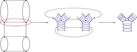
Figure 13: An example of non-admissible twist.

As is mentioned in subsection 2.1, we can decompose $\left|G_{g,n,\mathbf{L}}\right|$ into $2g-2+n$ pairs of pants by cutting it along along $3g-3+n$ essential simple closed curves. Each pair of pants inherits the measured foliation which is equivalent to that of $\left|G_{0,3,(L_{1},L_{2},L_{3})}\right|$ for some $L_{1},L_{2},L_{3}$. On the other hand, if we glue surfaces of the form $\left|G_{0,3,\cdot}\right|$ with the measured foliations in a measure preserving way, we cannot get a surface of the form $\left|G_{g,n,\mathbf{L}}\right|$ for some choice of twists. Such a twist is called a non-admissible twist.

An example of such a twist is illustrated in Figure 13. Let us consider two dumbbell type combinatorial pairs of pants of the same shape and glue them with the zero twist as shown in the figure. The thickened pairs of pants are glued in the way so that the foliation develops leaves connecting singular points and a part of the surface looks like a closed string propagator. Such a foliation cannot come from a metric ribbon graph.

References

- [1] K. Strebel, Quadratic differentials. Springer, 1984.
- [2] M. Saadi and B. Zwiebach, “Closed string field theory from polyhedra,” Annals Phys. 192 (1989) 213.
- [3] T. Kugo, H. Kunitomo, and K. Suehiro, “Nonpolynomial closed string field theory,” Phys. Lett. B 226 (1989) 48–54.
- [4] T. Kugo and K. Suehiro, “Nonpolynomial closed string field theory: Action and its gauge invariance,” Nucl. Phys. B 337 (1990) 434–466.
- [5] B. Zwiebach, “Consistency of closed string polyhedra from minimal area,” Phys. Lett. B 241 (1990) 343–349.
- [6] B. Zwiebach, “How covariant closed string theory solves a minimal area problem,” Commun. Math. Phys. 136 (1991) 83–118.
- [7] B. Zwiebach, “Closed string field theory: Quantum action and the Batalin-Vilkovisky master equation,” Nucl. Phys. B 390 (1993) 33–152, arXiv:hep-th/9206084.
- [8] S. F. Moosavian and R. Pius, “Hyperbolic geometry and closed bosonic string field theory. part I. the string vertices via hyperbolic Riemann surfaces,” JHEP 08 (2019) 157, arXiv:1706.07366 [hep-th].
- [9] S. F. Moosavian and R. Pius, “Hyperbolic geometry and closed bosonic string field theory. part II. the rules for evaluating the quantum BV master action,” JHEP 08 (2019) 177, arXiv:1708.04977 [hep-th].
- [10] K. Costello and B. Zwiebach, “Hyperbolic string vertices,” JHEP 02 (2022) 002, arXiv:1909.00033 [hep-th].
- [11] N. Ishibashi, “The Fokker-Planck formalism for closed bosonic strings,” PTEP 2023 (2023) no. 2, 023B05, arXiv:2210.04134 [hep-th].
- [12] M. Mirzakhani, “Simple geodesics and Weil-Petersson volumes of moduli spaces of bordered Riemann surfaces,” Invent. Math. 167 (2006) no. 1, 179–222.
- [13] M. Mirzakhani, “Weil-Petersson volumes and intersection theory on the moduli space of curves,” J. Am. Math. Soc. 20 (2007) no. 01, 1–24.
- [14] J. Bennett, D. Cochran, B. Safnuk, and K. Woskoff, “Topological recursion for symplectic volumes of moduli spaces of curves,” Michigan Mathematical Journal 61 (2012) no. 2, 331–358.
- [15] J. E. Andersen, G. Borot, S. Charbonnier, A. Giacchetto, D. Lewański, and C. Wheeler, “On the Kontsevich geometry of the combinatorial Teichmüller space,” arXiv preprint arXiv:2010.11806 (2020) .
- [16] M. Kontsevich, “Intersection theory on the moduli space of curves and the matrix Airy function,” Communications in Mathematical Physics 147 (1992) 1–23.
- [17] A. H. Fırat, “Hyperbolic three-string vertex,” JHEP 08 (2021) 035, arXiv:2102.03936 [hep-th].
- [18] A. H. Fırat, “Bootstrapping closed string field theory,” JHEP 05 (2023) 186, arXiv:2302.12843 [hep-th].
- [19] G. Mondello, “Riemann surfaces with boundary and natural triangulations of the Teichmüller space,” Journal of the European Mathematical Society 13 (2011) no. 3, 635–684.
- [20] G. Mondello, “Triangulated Riemann surfaces with boundary and the Weil-Petersson Poisson structure,” Journal of Differential Geometry 81 (2009) no. 2, 391–436.
- [21] N. Do, “The asymptotic Weil-Petersson form and intersection theory on ,” arXiv preprint arXiv:1010.4126 (2010) .
- [22] E. Witten, “Noncommutative geometry and string field theory,” Nucl. Phys. B 268 (1986) 253–294.
- [23] W. P. Thurston, “On the geometry and dynamics of diffeomorphisms of surfaces,” Bulletin of the American mathematical society 19 (1988) no. 2, 417–431.
- [24] A. Fathi, F. Laudenbach, and V. Poénaru, Thurston’s Work on Surfaces (MN-48), vol. 48. Princeton University Press, 2021.
- [25] R. C. Penner and J. L. Harer, Combinatorics of train tracks. No. 125. Princeton University Press, 1992.
- [26] A. Sen, “Off-shell amplitudes in superstring theory,” Fortsch. Phys. 63 (2015) 149–188, arXiv:1408.0571 [hep-th].
- [27] C. de Lacroix, H. Erbin, S. P. Kashyap, A. Sen, and M. Verma, “Closed superstring field theory and its applications,” Int. J. Mod. Phys. A 32 (2017) no. 28n29, 1730021, arXiv:1703.06410 [hep-th].
- [28] T. Erler, “Four lectures on closed string field theory,” Phys. Rept. 851 (2020) 1–36, arXiv:1905.06785 [hep-th].
- [29] H. Erbin, String Field Theory: A Modern Introduction, vol. 980 of Lecture Notes in Physics. 3, 2021.
- [30] G. McShane, “A remarkable identity for lengths of curves,” Ph. D. thesis, University of Warwick (1991) .
- [31] N. Ishibashi and H. Kawai, “String field theory of noncritical strings,” Phys. Lett. B 314 (1993) 190–196, arXiv:hep-th/9307045.
- [32] A. Jevicki and J. P. Rodrigues, “Loop space Hamiltonians and field theory of noncritical strings,” Nucl. Phys. B 421 (1994) 278–292, arXiv:hep-th/9312118.
- [33] N. Ishibashi and H. Kawai, “String field theory of noncritical strings,” Phys. Lett. B 322 (1994) 67–78, arXiv:hep-th/9312047.
- [34] M. Ikehara, N. Ishibashi, H. Kawai, T. Mogami, R. Nakayama, and N. Sasakura, “String field theory in the temporal gauge,” Phys. Rev. D 50 (1994) 7467–7478, arXiv:hep-th/9406207.
- [35] M. Ikehara, N. Ishibashi, H. Kawai, T. Mogami, R. Nakayama, and N. Sasakura, “A note on string field theory in the temporal gauge,” Prog. Theor. Phys. Suppl. 118 (1995) 241–258, arXiv:hep-th/9409101.
- [36] A. Sen, “Reality of superstring field theory action,” JHEP 11 (2016) 014, arXiv:1606.03455 [hep-th].
- [37] R. Gopakumar, “From free fields to AdS. III,” Phys. Rev. D 72 (2005) 066008, arXiv:hep-th/0504229.
- [38] F. Bhat, R. Gopakumar, P. Maity, and B. Radhakrishnan, “Twistor coverings and Feynman diagrams,” JHEP 05 (2022) 150, arXiv:2112.05115 [hep-th].
- [39] Y. Okawa and B. Zwiebach, “Twisted tachyon condensation in closed string field theory,” JHEP 03 (2004) 056, arXiv:hep-th/0403051.
- [40] H. Yang and B. Zwiebach, “A closed string tachyon vacuum?,” JHEP 09 (2005) 054, arXiv:hep-th/0506077.
- [41] N. Moeller and H. Yang, “The nonperturbative closed string tachyon vacuum to high level,” JHEP 04 (2007) 009, arXiv:hep-th/0609208.
- [42] J. Scheinpflug and M. Schnabl, “Closed string tachyon condensation revisited,” arXiv:2308.16142 [hep-th].
- [43] A. S. Schwarz and A. M. Zeitlin, “Super Riemann surfaces and fatgraphs,” Universe 9 (2023) no. 9, 384.
- [44] M. Mulase and M. Penkava, “Ribbon graphs, quadratic differentials on Riemann surfaces, and algebraic curves defined over ," Asian Journal of Mathematics 2 (4),(1998) 875–920,” arXiv preprint math-ph/9811024 (1998) .