Supplementary materials: Minimal design of the elephant trunk as an active filament

Bartosz Kaczmarski, Sophie Leanza, Renee Zhao Department of Mechanical Engineering, Stanford University, Stanford, CA-94305, United States    Derek E. Moulton Mathematical Institute, University of Oxford, Oxford, UK    Ellen Kuhl Department of Mechanical Engineering, Stanford University, Stanford, CA-94305, United States    Alain Goriely Mathematical Institute, University of Oxford, Oxford, UK

Model set-up.—In the active filament formulae,

$$\begin{split}\hat{{\mathsf{u}}}_{1}&=-\frac{4}{3R_{0}^{4}}A\delta_{1}\sin\left(\varphi-\frac{Z}{R_{0}}\tan\alpha\right),\\ \hat{{\mathsf{u}}}_{2}&=-\frac{4}{3R_{0}^{4}}A\delta_{2}\cos\left(\varphi-\frac{Z}{R_{0}}\tan\alpha\right),\\ \hat{{\mathsf{u}}}_{3}&=\frac{2}{R_{0}^{4}}\delta_{3}a_{0},\quad\hat{\zeta}=1+\frac{1}{2R_{0}^{2}}\delta_{0}a_{0},\end{split}$$ (1)

the quantities $\delta_{0}$, $\delta_{1}$, $\delta_{2}$, and $\delta_{3}$ are functions of the filament geometry, fiber architecture, and the Poisson’s ratio of the filament material. As shown in [1], given a ring cross-section with an inner radius $R_{1}$ and an outer radius $R_{2}=R_{0}$, a fiber architecture with a constant helical angle $\alpha$, and a Poisson’s ratio $\nu$ of the structure, we have

$$\begin{split}\delta_{0}&=(\nu+1)R_{2}^{2}\cot^{2}\alpha\log\left(\frac{R_{2}^{2}\sec^{2}\!\alpha}{R_{1}^{2}\tan^{2}\alpha+R_{2}^{2}}\right)+\nu\left(R_{1}^{2}-R_{2}^{2}\right),\\ \delta_{1}&=\delta_{2}=\left(R_{1}-R_{2}\right)\left(\nu\left(R_{1}^{2}+R_{2}R_{1}+R_{2}^{2}\right)-3(\nu+1)R_{2}^{2}\cot^{2}\alpha\right)\\ &\phantom{\delta_{2}=\delta_{1}=}+3(\nu+1)R_{2}^{3}\cot^{3}\alpha\arctan\left(\frac{R_{1}\tan\alpha}{R_{2}}\right)-3\alpha(\nu+1)R_{2}^{3}\cot^{3}\alpha,\\ \delta_{3}&=-(1+\nu)R_{2}\cot\alpha\left(R_{1}^{2}-R_{2}^{2}+R_{2}^{2}\cot^{2}\alpha\log\left(\frac{2R_{2}^{2}}{\left(R_{2}^{2}-R_{1}^{2}\right)\cos 2\alpha+R_{1}^{2}+R_{2}^{2}}\right)\right).\end{split}$$ (2)

For longitudinal fibers, we take the limit $\alpha\rightarrow 0$, for which these expressions simplify to

$$\begin{split}\delta_{0}&=R_{2}^{2}-R_{1}^{2},\\ \delta_{1}&=\delta_{2}=R_{2}^{3}-R_{1}^{3},\\ \delta_{3}&=0.\end{split}$$ (3)

In the case of a tapered filament geometry with a tapering angle $\phi_{2}(Z)$ defined at the outer surface $R=R_{2}(Z)$ of the filament, and longitudinal fibers with $\alpha=0$, the $\delta_{0}$, $\delta_{1}$, $\delta_{2}$, and $\delta_{3}$ quantities then become

$$\begin{split}\delta_{0}&=4(R_{1}^{2}-R_{2}^{2})\nu-\frac{4(1+\nu)}{c_{\phi}^{2}}\log\left(\frac{1+R_{1}^{2}c_{\phi}^{2}}{1+R_{2}^{2}c_{\phi}^{2}}\right),\\ \delta_{1}&=\delta_{2}=4(R_{1}^{3}-R_{2}^{3})\nu+\frac{12(1+\nu)}{c_{\phi}^{3}}\left(\arctan(R_{1}c_{\phi})\right.\\ &\qquad\qquad\left.-\arctan(R_{2}c_{\phi})+(R_{2}-R_{1})c_{\phi}\right),\\ \delta_{3}&=0,\\ c_{\phi}&=c_{\phi}(Z)=\frac{\tan{(\phi_{2}(Z))}}{R_{2}(Z)}.\end{split}$$ (4)

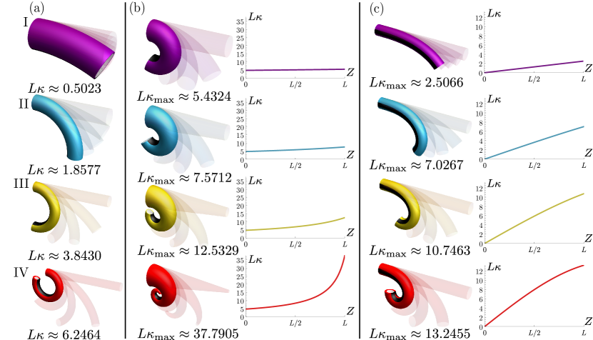
Curvatures in the parametric studies—In the parametric studies, we reported the dimensionless curvature $L\kappa$ for the case of varied slenderness $S_{\text{r}}$, and the maximal curvature $L\kappa_{\text{max}}$ for the cases in which the tapering angle $\phi$ and the fiber revolution $\Omega$ were varied. The reason for reporting the maximal curvature in the two latter scenarios is that the curvature itself varies along the length of the filament. To supplement the reported results, fig. S1 provides specific numerical values of $L\kappa$ and $L\kappa_{\text{max}}$ for the 12 evaluated designs, as well as the curvature functions $L\kappa(Z)$ for the tapering angle and fiber helicity studies shown in figs. S1b and S1c, respectively.

Refer to caption
Figure 1: Additional information regarding curvature values and curvature functions present for the 12 designs presented in the parametric studies. (a) Designs with different slenderness values. Since the curvature is constant along $Z$, just the values of $L\kappa$ are shown for the designs I-IV. (b) Designs with different tapering angles and (c) designs with different fiber revolution angles. The curvature varies along $Z$ in (b) and (c), so both the values of $L\kappa_{\text{max}}$ and the plots of $L\kappa$ vs. Z are shown for the four respective designs in each case.

Material properties of evaluated designs.—In parametric studies, the only mechanical property of the filament material whose value is significant for the reported results is the Poisson’s ratio $\nu$, which was chosen to be $\nu=1/2$ and homogeneous for all 12 designs. The Young’s modulus $E$ was also assumed to be homogeneous throughout the entire structure in those designs, which, according to the theory in [1], removes the dependence on the value of $E$ in $\hat{{\mathsf{u}}}_{1}$, $\hat{{\mathsf{u}}}_{2}$, $\hat{{\mathsf{u}}}_{3}$, and $\hat{\zeta}$ under the assumption of the ring solution.

However, for the comparison between the minimal design and the experimental results to be valid, the assumption of a homogeneous Young’s modulus and Poisson’s ratio is no longer valid since the LCE fiber bundles in the experimental prototype have different material properties than that of the surrounding elastic matrix.

Therefore, a minor adjustment to the model setup has to be made to account for material inhomogeneity in the minimal design. Let $E_{\text{f}}$ and $\nu_{\text{f}}$ denote the elastic modulus and Poisson’s ratio of the LCE fibers, and $E_{\text{M}}$ and $\nu_{\text{M}}$ denote the elastic modulus and Poisson’s ratio of the elastic matrix. Then, an approximation of the intrinsic curvatures $\hat{{\mathsf{u}}}_{1}$, $\hat{{\mathsf{u}}}_{2}$, $\hat{{\mathsf{u}}}_{3}$, and extension $\hat{\zeta}$ can be shown to be expressed as

$$\begin{split}\hat{{\mathsf{u}}}_{1}&\approx-\frac{4E_{\text{f}}}{3\left(E_{\text{M}}R_{1}^{4}+E_{\text{f}}(R_{0}^{4}-R_{1}^{4})\right)}A\delta_{1,\text{f}}\sin\left(\varphi-\frac{Z}{R_{0}}\tan\alpha\right),\\ \hat{{\mathsf{u}}}_{2}&\approx-\frac{4E_{\text{f}}}{3\left(E_{\text{M}}R_{1}^{4}+E_{\text{f}}(R_{0}^{4}-R_{1}^{4})\right)}A\delta_{2,\text{f}}\cos\left(\varphi-\frac{Z}{R_{0}}\tan\alpha\right),\\ \hat{{\mathsf{u}}}_{3}&\approx\frac{2E_{\text{f}}(1+\nu_{\text{M}})}{E_{\text{M}}R_{1}^{4}(1+\nu_{\text{f}})+E_{\text{f}}(R_{0}^{4}-R_{1}^{4})(1+\nu_{\text{M}})}\delta_{3,\text{f}}a_{0},\\ \hat{\zeta}&\approx 1+\frac{E_{\text{f}}}{2(E_{\text{M}}R_{1}^{2}+E_{\text{f}}(R_{0}^{2}-R_{1}^{2}))}\delta_{0,\text{f}}a_{0},\end{split}$$ (5)

where $\delta_{i,\text{f}}$ are defined as in Eqs. (2) and (4), but with the substitution $\nu\rightarrow\nu_{\text{f}}$. All other quantities are defined as before. The approximation stems from the simplifying assumption that the activated ring region shares the material properties of the LCE fibers, even if the LCE fibers do not make up the entirety of the activatable ring. The accuracy of this approximation increases as the size of the ring relative to the size of the elastic matrix decreases, and as the total angular extent of the LCE fibers in the ring approaches $2\pi$.

Multiple helical angles in a ring.—The minimal design consists of a longitudinal fiber bundle and two symmetrically arranged helical fiber bundles of opposite handedness. That is, $\alpha^{(1)}=0\neq\alpha^{(2)}\neq\alpha^{(3)}$ and $\alpha^{(2)}=-\alpha^{(3)}$, where $\alpha^{(1)}=0$ is the helical angle of the longitudinal fiber bundle, and $\alpha^{(2)}$, $\alpha^{(3)}$ are the helical angles of the two helical fiber bundles. However, Eq. (1) is posed in terms of a single angle $\alpha$. To be able to account for the contributions of all three fiber bundles, we can utilize the superposition property of the active filament model, which handles the mathematical treatment of multiple concentric rings of activation [1]. Similar to Eq. (5), for a general filament with $M$ concentric rings of activation and different material properties in the fibers of each ring and the elastic matrix, the resulting curvatures and extensions can be approximated as

$$\begin{split}\hat{{\mathsf{u}}}_{1}&\approx-\frac{4\sum_{i=1}^{M}E_{\text{f}}^{(i)}\delta_{1,\text{f}}^{(i)}A^{(i)}\sin\left(\varphi^{(i)}-\frac{Z}{R_{2}^{(i)}}\tan{\alpha^{(i)}}\right)}{3\left[E_{\text{M}}\left(R_{1}^{(1)}\right)^{4}+\sum_{i=1}^{M}E_{\text{f}}^{(i)}\left(\left(R_{2}^{(i)}\right)^{4}-\left(R_{1}^{(i)}\right)^{4}\right)\right]},\\ \hat{{\mathsf{u}}}_{2}&\approx-\frac{4\sum_{i=1}^{M}E_{\text{f}}^{(i)}\delta_{2,\text{f}}^{(i)}A^{(i)}\cos\left(\varphi^{(i)}-\frac{Z}{R_{2}^{(i)}}\tan{\alpha^{(i)}}\right)}{3\left[E_{\text{M}}\left(R_{1}^{(1)}\right)^{4}+\sum_{i=1}^{M}E_{\text{f}}^{(i)}\left(\left(R_{2}^{(i)}\right)^{4}-\left(R_{1}^{(i)}\right)^{4}\right)\right]},\\ \hat{{\mathsf{u}}}_{3}&\approx\frac{2\sum_{i=1}^{M}a_{0}^{(i)}E_{\text{f}}^{(i)}\delta_{3,\text{f}}^{(i)}\left(1+\nu_{\text{f}}^{(i)}\right)^{-1}}{E_{\text{M}}\left(R_{1}^{(i)}\right)^{4}\left(1+\nu_{\text{M}}\right)^{-1}+\sum_{i=1}^{M}E_{\text{f}}^{(i)}\left(\left(R_{2}^{(i)}\right)^{4}-\left(R_{1}^{(i)}\right)^{4}\right)\left(1+\nu_{\text{f}}^{(i)}\right)^{-1}},\\ \hat{\zeta}&\approx 1+\frac{\sum_{i=1}^{M}a_{0}^{(i)}E_{\text{f}}^{(i)}\delta_{0,\text{f}}^{(i)}}{2\left[E_{\text{M}}\left(R_{1}^{(i)}\right)^{2}+\sum_{i=1}^{M}E_{\text{f}}^{(i)}\left(\left(R_{2}^{(i)}\right)^{2}-\left(R_{1}^{(i)}\right)^{2}\right)\right]},\end{split}$$ (6)

where any quantity $(\cdot)^{(i)}$ is associated with the $i$-th activation ring in the filament, $i=1,\ldots,M$. The approximation is again the result of the assumption of constant material properties $E_{\text{f}}^{(i)}$, $\nu_{\text{f}}^{(i)}$ within a given ring, but different properties $E_{\text{M}}$, $\nu_{\text{M}}$ in the elastic matrix. We emphasize that, in the single-ring case, it was true that $R_{0}=R_{2}$ (outer radius of the whole structure is the outer radius of the single ring), but, in the $M$-ring case, we have $R_{0}=R_{2}^{(M)}$.

In the case of the minimal design, three rings are needed to represent the actuators utilizing the three different fiber architectures. All three rings have the same inner radius $R_{1}$ and outer radius $R_{2}$ since all three fiber bundles are contained within one ring region. Therefore, we can set $R_{1}^{(1)}=R_{1}^{(2)}=R_{1}^{(3)}=R_{1}$ and $R_{2}^{(1)}=R_{2}^{(2)}=R_{2}^{(3)}=R_{0}$. Further, the three fiber bundles have the same material properties, so $E_{\text{f}}^{(1)}=E_{\text{f}}^{(2)}=E_{\text{f}}^{(3)}=E_{\text{f}}$ and $\nu_{\text{f}}^{(1)}=\nu_{\text{f}}^{(2)}=\nu_{\text{f}}^{(3)}=\nu_{\text{f}}$, which simplifies the general expressions in Eq. (6).

The outlined procedure was also applied to the simpler case of the design with two symmetrically arranged helical fiber bundles in the parametric study of the fiber revolution parameter $\Omega$. In that scenario, we remove the longitudinal actuator ring and assume $E_{\text{M}}=E_{\text{f}}^{(i)}$, $\nu_{\text{M}}=\nu_{\text{f}}^{(i)}$, for $i=1,2$.

Definitions of tapering and fiber revolution—For a general tapering profile, we can define the tapering angle field as a function of the cylindrical radius coordinate $R$ and the parameter $Z$ as [1]

$\displaystyle\tan(\phi(R,Z))=\frac{R}{R_{2}(Z)}R_{2}^{\prime}(Z).$ (7)

Given that the tapering profile is assumed to be linear, it can be described with a single tapering angle prescribed for the whole design such that

$\displaystyle\tan(\phi(R=R_{2}))=\frac{R_{2}(L)-R_{2}(0)}{L},$ (8)

which is the definition used for the color bar in the parametric studies. The inner radius profile $R_{1}(Z)$ is then set to follow the tapering profile according to

$\displaystyle R_{1}(Z)=\frac{R_{1}(0)}{R_{2}(0)}R_{2}(Z).$ (9)

The fiber revolution angle $\Omega$ is the total angular revolution of the fiber for $Z\in[0,L]$. Given a helical angle $\alpha$, it is defined for an non-tapered structure as

$\displaystyle\Omega=\frac{L}{R_{2}}\tan{\alpha}.$ (10)

Using the fiber revolution angle for design purposes is the most intuitive as it allows direct reasoning about fiber interpenetration when multiple helical fibers are present.

Stiffness correction for overlapping rings—The actuators of the minimal design are represented with three activation rings with the same inner and outer radii. Thus, the rings overlap fully with one another, which results in overcounting of the stiffness contributions from $E_{\text{f}}$ in each of the overlapping rings, while there is only one physical ring region. As such, we use a simple stiffness correction that addresses this overcounting issue. Since the stiffness is overcounted $M$ times for an $M$-ring filament, a simple scaling by $k_{\text{count}}=1/M$ is sufficient, so that the corrected Young’s modulus is $\tilde{E}_{\text{count}}^{(i)}=k_{\text{count}}E_{\text{f}}$ for the $i$-th ring.

Stiffness correction for the comparison with experimental results—The fabricated experimental prototype involves LCE fiber bundles that adhere to the outer surface of the tubular elastic matrix. In the context of the ring solution in the active filament model, this effectively introduces empty space between the activated angular sectors of the ring. By default, however, the model assumes that the elastic matrix also fills the space between the fiber bundles within the ring, since the derivation of the curvature and extension formulae is not straightforward for the case of a Young’s modulus that is variable and discontinuous in the polar angle. Thus, we performed a stiffness averaging operation, so that the adjusted axial stiffness matches the axial stiffness of the ring with the empty space that is present in the experimental setup.

Specifically, consider the $i$-th ring of the filament with a Young’s modulus $E_{\text{f}}$ and with its default definition under the active filament model (filled space between fiber bundles). Its axial stiffness is

$\displaystyle K_{0}^{(i)}=E_{\text{f}}\pi((R_{2}^{(i)})^{2}-(R_{1}^{(i)})^{2}).$ (11)

Now, for a piecewise-constant activation pattern $\gamma^{(i)}(\theta)$ that defines a set of $N^{(i)}$ discrete fiber bundles with angular extents $\sigma^{(i)}$ in the $i$-th ring, the axial stiffness of the ring that accounts for the empty space is

$\displaystyle\tilde{K}_{0}^{(i)}=\frac{N^{(i)}\sigma^{(i)}}{2\pi}K_{0}^{(i)},$ (12)

which means that the scaling factor for the Young’s modulus of the $i$-th ring could be chosen as $k_{\text{empty}}^{(i)}=N^{(i)}\sigma^{(i)}/2\pi$, so that the corrected Young’s modulus is $\tilde{E}_{\text{empty}}^{(i)}=k_{\text{empty}}^{(i)}E_{\text{f}}$.

We combine the stiffness correction for overlapping rings with the empty-space stiffness correction, which gives the final corrected Young’s modulus

$\displaystyle\tilde{E}_{\text{f}}=\left(k_{\text{count}}\sum_{i=1}^{M}k_{\text{empty}}^{(i)}\right)E_{\text{f}}.$ (13)

For consistency, this combined correction was also employed in the generation of the reachability clouds in addition to its use in the comparison with experimental deformations, given that the same actuator design is used in both results.

Note that the discussed stiffness corrections are not relevant to the parametric study of the fiber revolution angle, since that scenario assumes a homogeneous Young’s modulus throughout the filament, i.e., $E_{\text{M}}=E_{\text{f}}$, which removes the dependence of the curvature and extension functions on the Young’s modulus. Particularly, the stiffness overcounting is not manifested in that case, even though two overlapping helical rings are used. There is also no need to apply the empty-space correction, as the default active filament representation is appropriate for reasoning about the fiber helicity effects.

Minimal design parameter details—The minimal design consists of a filament of length $L=0.09\,\text{m}$ and an outer radius $R_{0}=L/20$, in which the activatable ring has a constant outer radius $R_{2}=R_{0}=L/20$ and a constant inner radius $R_{1}=(5/6)R_{2}$. The piecewise-constant activation pattern in the ring defines a set of three fiber bundles with angular extents $\sigma=48^{\circ}$. Two of the fiber bundles are helical with opposite handedness (red and green actuators), and start with angular phase offsets $\theta_{0,\text{red}}=66^{\circ}$ and $\theta_{0,\text{green}}=114^{\circ}$ in the cross section at $Z=0$. The third fiber bundle (blue actuator) is longitudinal and starts at an angle offset $\theta_{0,\text{blue}}=270^{\circ}$ in the cross section. The fiber revolutions of the helical fiber bundles are set such that they just meet (and not interpenetrate) the longitudinal fiber bundle at $Z=L$, which means that $\Omega_{\text{red}}=-108^{\circ}$ and $\Omega_{\text{green}}=108^{\circ}$. These give rise to helical angles $\alpha_{\text{red}}\approx-0.756$ and $\alpha_{\text{green}}\approx 0.756$.

The material properties of the minimal design are set to match the experimental setup in the experimental validation step. In particular, we set

$$\begin{split}E_{\text{f}}&=1.4\,\text{MPa},\\ \nu_{\text{f}}&=0.495,\\ E_{\text{M}}&=127.8\,\text{kPa},\\ \nu_{\text{M}}&=0.5,\end{split}$$ (14)

and a volumetric density $\rho_{\text{vol}}=1000\text{kg}/\text{m}^{3}$.

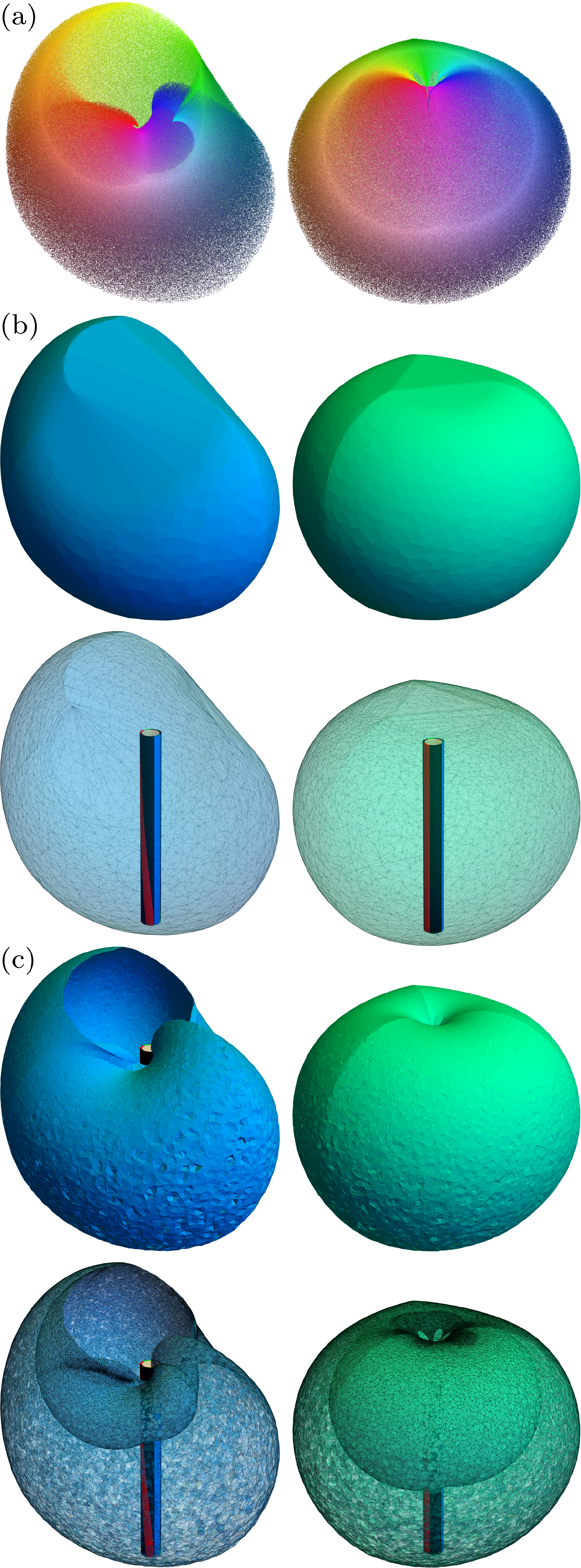
Reachability cloud volume—The task of establishing the volumetric coverage of an arbitrary point cloud is generally non-trivial. We estimated the upper bound of the reachability cloud volume as the volume of the convex hull bounding the 2 million endpoints of the deformed design. Further, we estimated the minimal non-convex volume spanned by the reachability cloud by constructing the concave hull mesh of the 3D data using the $\alpha$-shapes method [2]. Both the convex and the concave hulls are visualized in Fig. S2 for both the minimal design and the design with 3 longitudinal fiber bundles.

Refer to caption
Figure 2: Convex and concave hulls of the reachability clouds of the minimal design (left) and the design with 3 longitudinal fiber bundles (right). (a) The discrete reachability point cloud of deformed design endpoints obtained through uniform sampling $\gamma_{i}\in[-5,0]$. (b) The convex hull of the cloud which gives the upper bound for the cloud volume. (c) Concave hull mesh that wraps around the topologically complex, non-convex structure of the cloud. The initial configurations are shown in the translucent visualizations of the hull meshes.

Muscle strains in the minimal design—To compare the activation magnitudes $|\gamma_{i}|$ to muscular contraction levels observed physiologically in elephant trunks, we used a measure of deformed fiber strain during a simple in-plane bending motion of the minimal design with only the longitudinal bundle activated. An estimate of the deformed fiber strain in the deformed configuration can be computed as $(L_{\mathcal{F}}^{1}/L_{\mathcal{F}}^{0})-1$, where $L_{\mathcal{F}}^{0}$ is the initial total arc length of the fiber $\mathcal{F}$ and $L_{\mathcal{F}}^{1}$ is its deformed total arc length. For a given filament configuration $\{\mathbf{r}(Z),\mathbf{d}_{1}(Z),\mathbf{d}_{2}(Z),\mathbf{d}_{3}(Z)\}$, the total arc length of a fiber with initial phase offset $\theta_{0}$, helical angle $\alpha$, and outer radius $R_{2}$ can be computed as

$\displaystyle L_{\mathcal{F}}$ $\displaystyle=\int_{0}^{L}\left\|\frac{\partial}{\partial Z}\left[\mathbf{r}(Z)+R_{2}\left(\mathbf{d}_{1}\cos\left(\theta_{0}+\frac{Z}{R_{2}}\tan\alpha\right)\right.\right.\right.$
$\displaystyle\hskip 42.67912pt\left.\left.\left.+\;\mathbf{d}_{2}\sin\left(\theta_{0}+\frac{Z}{R_{2}}\tan\alpha\right)\right)\right]\right\|\,dZ.$ (15)

For the minimal design, this gives an estimate of $|\gamma_{3}|\approx 3.33$ that results in a fibrillar contraction of $33\%$ in the longitudinal bundle for the pure-bending deformation.

Filament integration with gravitational forces—To compute the deformation of the activated filament under the influence of gravitational forces due to its own weight, we treat the filament as an extensible, unshearable Kirchhoff rod governed by a constitutive law for an isotropic material with a quadratic energy form. This construction is adapted from [3] for the specific case of integration under self-weight.

Let us first specify three configurations utilized in the theory: the initial configuration (pre-activation), the reference configuration (post-activation) and the deformed configuration (post-activation and with external loading). The arc length parameters for the three configurations are $Z$, $S$, and $s$, respectively. The extension in the reference configuration is $\hat{\zeta}=dS/dZ$, and the extension in the deformed configuration due to external forces is $\zeta_{\mathbf{F}}=ds/dS$.

Under the influence of gravitational acceleration $\mathbf{g}$, the filament is subject to an external body force per unit length in the deformed configuration $\rho\mathbf{g}$, where $\rho$ is the linear density of the filament in the deformed configuration. This gives

$\displaystyle\frac{\partial\mathbf{n}}{\partial s}+\rho\mathbf{g}$ $\displaystyle=\mathbf{0}$ (16)

for the balance of the internal force $\mathbf{n}$ in the deformed configuration. Now, given that $ds/dZ=(ds/dS)(dS/dZ)=\zeta_{\mathbf{F}}\hat{\zeta}$, we can write

$\displaystyle\frac{\partial\mathbf{n}}{\partial Z}+\hat{\zeta}\zeta_{\mathbf{F}}\rho\mathbf{g}$ $\displaystyle=\mathbf{0}.$ (17)

Further, an infinitesimal element of mass $dm$ and density $\rho_{0}$ in the initial configuration is mapped to an element with the same mass and different density $\rho$ in the deformed configuration, such that

$\displaystyle dm=\rho\,ds=\rho\hat{\zeta}\zeta_{\mathbf{F}}\,dZ=\rho_{0}\,dZ\Rightarrow\rho=\frac{\rho_{0}}{\hat{\zeta}\zeta_{\mathbf{F}}}$ (18)

Thus,

$\displaystyle\frac{\partial\mathbf{n}}{\partial Z}+\rho_{0}\mathbf{g}$ $\displaystyle=\mathbf{0},$ (19)

which, given that $\mathbf{n}(L)=\mathbf{0}$, yields the internal force

$\displaystyle\mathbf{n}(Z)=\mathbf{g}\int_{Z}^{L}\rho_{0}(Z^{\prime})\,dZ^{\prime}.$ (20)

Assuming a non-tapered filament with homogeneous volumetric density ($\rho_{0}$ becomes constant) and that $\mathbf{g}=-g\mathbf{e}_{Z}$, we obtain the following components of $\mathbf{n}$ expressed in the local basis:

$\displaystyle\mathsf{n}_{i}(Z)=g\rho_{0}(Z-L)(\mathbf{d}_{i}\cdot\mathbf{e}_{Z}).$ (21)

The general moment balance for the filament can be expressed in the deformed configuration as

$\displaystyle\frac{\partial\mathbf{m}}{\partial s}+\frac{\partial\mathbf{r}}{\partial s}\times\mathbf{n}+\zeta_{\mathbf{F}}^{-1}\mathbf{l}$ $\displaystyle=\mathbf{0},$ (22)

where $\mathbf{m}$ is the internal moment, and $\zeta_{\mathbf{F}}^{-1}\mathbf{l}$ is the couple per unit length in the deformed configuration. For gravitational loading, we have $\mathbf{l}=\mathbf{0}$, so we can write the components of the moment $\mathbf{m}$ in the local basis as

$$\begin{split}\mathsf{m}_{1}^{\prime}(Z)&=\hat{\zeta}(\mathsf{u}_{3}(Z)\mathsf{m}_{2}(Z)-\mathsf{u}_{2}(Z)\mathsf{m}_{3}(Z))+\zeta\mathsf{n}_{2}(Z),\\ \mathsf{m}_{2}^{\prime}(Z)&=\hat{\zeta}(\mathsf{u}_{1}(Z)\mathsf{m}_{3}(Z)-\mathsf{u}_{3}(Z)\mathsf{m}_{1}(Z))-\zeta\mathsf{n}_{1}(Z),\\ \mathsf{m}_{3}^{\prime}(Z)&=\hat{\zeta}(\mathsf{u}_{2}(Z)\mathsf{m}_{1}(Z)-\mathsf{u}_{1}(Z)\mathsf{m}_{2}(Z)),\end{split}$$ (23)

where $\zeta=\zeta_{\mathbf{F}}\hat{\zeta}$ is the overall extension of the rod. The deformed curvatures $\mathsf{u}_{i}$ are derived from the intrinsic curvatures as

$\displaystyle\mathsf{u}_{i}(Z)$ $\displaystyle=\hat{\mathsf{u}}_{i}(Z)+\frac{\mathsf{m}_{i}(Z)}{K_{i}},$ (24)

where $K_{i}$ are the stiffness coefficients of the rod about $\mathbf{d}_{i}$, for $i=1,2,3$.

To construct the extension $\zeta_{\mathbf{F}}$ due to the external loading, we use the constitutive relationship

$$\begin{split}\mathsf{n}_{3}(Z)=K_{0}(\zeta_{\mathbf{F}}(Z)-1).\end{split}$$ (25)

Finally, the deformed configuration of the rod is obtained by solving the boundary value problem

$$\begin{split}\mathbf{r}^{\prime}(Z)&=\zeta(Z)\mathbf{d}_{3}(Z),\\ \mathbf{d}_{i}^{\prime}(Z)&=\hat{\zeta}(Z)\mathbf{u}(Z)\times\mathbf{d}_{i}(Z),\quad i\in\{1,2,3\},\\ \mathsf{m}_{1}^{\prime}(Z)&=\hat{\zeta}(\mathsf{u}_{3}(Z)\mathsf{m}_{2}(Z)-\mathsf{u}_{2}(Z)\mathsf{m}_{3}(Z))+\zeta\mathsf{n}_{2}(Z),\\ \mathsf{m}_{2}^{\prime}(Z)&=\hat{\zeta}(\mathsf{u}_{1}(Z)\mathsf{m}_{3}(Z)-\mathsf{u}_{3}(Z)\mathsf{m}_{1}(Z))-\zeta\mathsf{n}_{1}(Z),\\ \mathsf{m}_{3}^{\prime}(Z)&=\hat{\zeta}(\mathsf{u}_{2}(Z)\mathsf{m}_{1}(Z)-\mathsf{u}_{1}(Z)\mathsf{m}_{2}(Z)),\\ \mathbf{r}(0)&=\mathbf{r}_{0},\\ \mathbf{d}_{i}(0)&=\mathbf{d}_{i0},\quad i\in\{1,2,3\},\\ \mathbf{m}(L)&=\mathbf{0},\end{split}$$ (26)

where $\mathbf{r}_{0}$, and $\mathbf{d}_{i0}$ define the clamped boundary condition. The BVP is solved using a shooting method and the Verner’s 7(6) Runge-Kutta method for the integration step [4]. Continuation is used through iterative scaling of the gravitational acceleration $g$ and reusing the previous BVP solution at each iteration.

Experimental methods—To fabricate the LCE ink, liquid crystal mesogens (2-Methyl-1,4-phenylene bis(4-((6-(acryloyloxy)hexyl)oxy)benzoate)) (RM 82, BOC Sciences, USA) and (1,4-Bis-[4-(3-acryloyloxypropyloxy)benzoyloxy]-2-methylbenzene) (RM 257, BOC Sciences, USA) are mixed in a weight ratio of 2.7:1. Next, the spacers, (2,2-(Ethylenedioxy)diethanethiol) (EDDET, Sigma Aldrich, USA) and (2,6-Di-tert-butyl-4-methylphenol) (BHT, Sigma Aldrich, USA) are added at 22.5 wt% and 2.25 wt% to the total weight of mesogens. After melting all components at 80°C for 45 min, the catalyst triethylamine (TEA, Sigma Aldrich, USA) and photoinitiator Irgacure 819 (Sigma Aldrich, USA) are added at 1.6 wt% and 1.8 wt%, respectively, to the total weight of mesogens. The mixture is stirred for 3 min with a magnetic stir bar at 80°C, then oligomerized in an oven at 80°C for 15 min, and next transferred to a 10 mL syringe barrel (Nordson EFD, USA), and heated again in a vacuum oven at 80°C for 20 min. The ink is finally defoamed in a planetary mixer (AR-100, Thinky, USA) at 2200 rpm for 6 min to remove trapped air. A customized three-dimensional (3D) printer is used for printing of the LCE fibers. 90 mm-long fibers with longitudinal alignment, a width of 1.7 mm, and thickness of 0.4 mm are printed. 44 AWG (0.050 mm diameter) copper wire is coiled, with coil diameter of 0.5 mm, and stretched such that there are 0.68 coils/mm along the fiber. Two rows of coiled copper wires are embedded in each LCE fiber, and the fibers are then cured with UV light for 10 min. The Young’s modulus of the cured LCE is measured to be 1.4 MPa.

The liquid resin for the inactive polymer rod is created by mixing butyl acrylate (Sigma Aldrich, USA), a commercial UV-curable phenoxyethyl acrylate monomer (Ebecryl 114, Allnex, USA), and a commercial UV-curable urethane oligomer (Ebecryl 8413, Allnex, USA) in a weight ratio of 12:7:1. Photoinitiator Irgacure 819 (Sigma Aldrich, USA) is added at 2 wt% to the total weight of the resin, and the resin is mixed for 10 min at 80°C until homogeneous. The shear modulus of this inactive polymer upon curing is estimated as 42.6 kPa, using a neo-Hookean fit of tensile test data.

Silicone molds are created in order to fabricate the soft actuator. The mold is an inverse of the soft actuator design; it includes the cavity of a 4 mm diameter by 90 mm long cylinder with 0.4 mm thick slots along the cylinder, two patterned helically with opposite handedness and one patterned longitudinally. By inserting the fabricated LCE fibers into the slots in the mold, the orientation of the LCE fibers is fixed. The inactive polymer resin is then poured into the mold and UV light is shined on the semi-transparent mold for 15 minutes. During this time, the inactive rod cures while also bonding to the LCE fibers. Once removed from the mold, the soft actuator is fully fabricated. Currents between 0.9A and 1A are applied to the copper wires in the respective LCE fibers for the experimental implementations shown in Fig. 5.

References

  • Kaczmarski et al. [2022] B. Kaczmarski, D. E. Moulton, E. Kuhl, and A. Goriely, Journal of the Mechanics and Physics of Solids 164, 104918 (2022).
  • Edelsbrunner et al. [1983] H. Edelsbrunner, D. Kirkpatrick, and R. Seidel, IEEE Transactions on Information Theory 29, 551 (1983).
  • Moulton et al. [2012] D. E. Moulton, T. Lessinnes, and A. Goriely, J. Mech. Phys. Solids 61, 398 (2012).
  • Verner [2010] J. H. Verner, Numerical Algorithms 53, 383 (2010).