MCMC-driven learning

Alexandre Bouchard-Côté (bouchard@stat.ubc.ca)
Trevor Campbell (trevor@stat.ubc.ca)
Geoff Pleiss (geoff.pleiss@stat.ubc.ca)
Nikola Surjanovic (nikola.surjanovic@stat.ubc.ca)

1.1 Introduction

Markov chain Monte Carlo (MCMC) is a general computational methodology for obtaining approximate draws from a target probability distribution $\pi$ by simulating a Markov chain with stationary distribution $\pi$. Historically, MCMC has been used mostly in situations with a fixed target distribution $\pi$ that admits pointwise density evaluation up to a constant; this is the usual case for Bayesian posterior inference, which is one of the most fruitful application areas for MCMC. Similarly, the majority of MCMC research in computational statistics has used a fixed Markov kernel $\kappa$.

In the last two decades, MCMC has been increasingly used in situations where either the target $\pi$, the kernel $\kappa$, or both involve parameters $\phi\in\Phi\subset\mathbb{R}^{m}$ that are tuned based on the generated Markov chain sequence. Originally this research area was driven by work on adaptive MCMC methods [7] whose goal was still to take draws from a fixed target $\pi$, but with an adaptive kernel $\kappa_{\phi}$ in the interest of improved mixing. Adaptivity arose from either varying scale/step size parameters in traditional kernels [53, 5, 105], by adding parametrized families to generate independent proposals [72], or as a surrogate for fast proposal generation [97]. Connections to the stochastic approximation literature (first noted by Andrieu & Robert [6]), and more recently advances from machine learning (ML), have created the need to study and develop MCMC methods in situations where both the kernel $\kappa_{\phi}$ and target $\pi_{\phi}$ may be adaptive, and the goal is not just to produce samples from $\pi_{\phi}$ but perhaps also to minimize some cost associated with $\phi$—often a discrepancy between $\pi_{\phi}$ and some other target $\pi$.

The goal of this chapter is to unify all of these problems—which encompass black-box variational inference [16, 66, 96, 131], adaptive MCMC [7], normalizing flow construction and transport-assisted MCMC [10, 42, 54, 73, 111, 129], surrogate-likelihood MCMC [60, 74, 128], coreset construction for MCMC with big data [21, 22, 23, 29, 30, 56, 71, 82], Markov chain gradient descent [115], Markovian score climbing [62, 81], and more; see Table 1.1—within one common framework, so that theory and methods developed for each may be translated and generalized. To unify this wide range of seemingly different MCMC/ML tasks, we introduce the notion of a Markovian optimization-integration (MOI) problem, which involves finding $\phi\in\Phi\subset\mathbb{R}^{m}$ such that

$$\addcontentsline{lla}{section}{\numberline{\string\crtrefnumber{eq:key}}{e}q:key}g(\phi):=\mathbb{E}_{\pi_{\phi}}\left[g(X,\phi)\right]=0,$$ (1.2)

where we do not have access to i.i.d. draws $X\in{\mathcal{X}}$ from $\pi_{\phi}$, but rather for each $\phi\in\Phi$ we are able to simulate from a $\pi_{\phi}$-invariant Markov chain with transition kernel $\kappa_{\phi}$ [14]. We are often motivated by cases where $g:{\mathcal{X}}\times\Phi\to\mathbb{R}^{m^{\prime}}$ in Eq. 1.2 is the gradient of a function that we seek to optimize, i.e., $g(x,\phi)=-\nabla_{\phi}f(x,\phi)$ for an objective $f$, and we are interested in solving

$$\addcontentsline{lla}{section}{\numberline{\string\crtrefnumber{eq:min}}{e}q:min}\min_{\phi}f(\phi).\qquad f(\phi):=\mathbb{E}_{\pi_{\phi}}\left[f(X,\phi)\right].$$ (1.3)

As we illustrate in this chapter, MOI problems of the form Eqs. 1.2 and 1.3 capture a wide range of both well-established and cutting-edge research areas at the intersection of MCMC and ML. For example, standard Bayesian variational inference—i.e., minimization of the reverse KL divergence $\mathrm{D_{KL}}(q_{\phi}||\pi)=\int\log\frac{q_{\phi}(x)}{\pi(x)}q_{\phi}(x)\,\mathrm{d}x$ within a family $q_{\phi}\in{\mathcal{Q}}$ that admits i.i.d. draws—can be seen as an MOI problem by setting $f(\phi)=\mathrm{D_{KL}}(q_{\phi}||\pi)$ and $\pi_{\phi}=q_{\phi}$ in Eq. 1.3. But so can more challenging settings, such as minimization of the reverse KL divergence when $q_{\phi}$ does not admit i.i.d. draws (as in coreset construction [29]), or minimization of the forward KL divergence, by setting $f(\phi)=\mathrm{D_{KL}}(\pi||q_{\phi})$ and $\pi_{\phi}=\pi$ in Eq. 1.3 [62, 81, 117].

By unifying these problems under the MOI framework, we see commonalities among the optimization procedures used to solve them. Existing algorithms designed for specific MOI problems can often be cast as variants of the adaptive algorithm

$$\addcontentsline{lla}{section}{\numberline{\string\crtrefnumber{eq:rm}}{e}q:rm}\phi_{t+1} =\phi_{t}+\gamma_{t}g(X_{t},\phi_{t})$$ (1.4)

$$X_{t+1} \sim\kappa_{\phi_{t+1}}(\cdot|X_{t}),$$ (1.5)

where $\gamma_{t}$ is the step size at iteration $t\geq 0$ and $\kappa_{\phi}$ is a Markov kernel that targets $\pi_{\phi}$. This algorithm, and in particular the convergence of the parameters $\phi_{t}$, has been studied extensively for the general setup in Eq. 1.2 [4, 5, 8, 14]. But this chapter also highlights deviations from this general formula, both in terms of the algorithmic approach [117] and the theoretical analysis techniques used to demonstrate convergence [29] for specific instances of Eq. 1.2.

The chapter concludes with a detailed exploration of a case of particular interest: distribution approximation via minimization of the forward KL divergence $f(\phi)=\mathrm{D_{KL}}(\pi||q_{\phi})$. Traditionally, the forward KL has not been considered in divergence minimization problems due to the inavailability of i.i.d. draws from $\pi$, making the minimization of this divergence generally more difficult. However, the forward KL is of particular interest because it has the property that it is mass covering; for instance, in the case of a multimodal distribution $\pi$, an optimal approximating distribution $q_{\phi^{\star}}$ under the forward KL would generally avoid undesirable mode collapse. Our example first considers training $q_{\phi}$ for use within an independence Metropolis–Hastings (IMH) proposal. We then generalize IMH to the case of variational parallel tempering [117], which targets distributions along an annealing path $q_{\phi}^{1-\beta}\cdot\pi^{\beta}$ for $0\leq\beta\leq 1$; here the forward KL is particularly desirable to minimize as it is known to control performance [117, 121].

This chapter is organized as follows. In Section 1.2, we list important examples of MOI problems, mapping them onto Eqs. 1.2 and 1.3. Next, in Section 1.3, we cover general strategies for solving MOI problems in greater detail, and in Section 1.4 we present theoretical results on stability and convergence. Because the MOI framework unifies many different algorithms at the intersection of MCMC and ML, the accompanying theory can therefore be applied to a wide range of problems. Finally, in Section 1.5, we work through a case study introducing several ideas and highlighting techniques previously presented in the chapter. We end with a discussion in Section 1.6 and a summary of suggested further reading in Section 1.7.

Table 1.1: Common MOI problems and a classification of the primary aspect of interest: either samples from $\pi$ (sampling problem) and/or an approximation $q_{\phi}$ of $\pi$ (optimization problem). Optional settings are indicated by $\sim$. $\star$ denotes a problem described in detail in Section 1.5.

Problem		Sampling problem?	Optimization problem?	Adaptive $\kappa_{\phi}$?	Adaptive $\pi_{\phi}$?
Black-box VI [16, 66, 96, 131]			✓	✓	✓
Forward KL VI/Score climbing$\star$ [62, 81]			✓	$\sim$	$\sim$
Adaptive MCMC [7]		✓		✓
Transport-assisted MCMC [10, 42, 54, 73, 111, 129]		✓	✓	$\sim$	$\sim$
Surrogate-likelihood MCMC [60]		✓		✓	✓
Coreset MCMC [21, 22, 23, 29, 30, 56, 71, 82]		✓	✓	✓	✓
Markov chain gradient descent [115]			✓
Variational parallel tempering$\star$ [117, 121]		✓	✓	✓	✓

1.2 Examples of MOI problems

We give an overview of various problems that have the MOI mathematical structure, given by Eq. 1.2 and Eq. 1.3, in order to motivate and emphasize the prevalence of such problems. A summary is provided in Table 1.1.

Forward KL variational inference

Bayesian variational inference (see, e.g., [16, 66, 96, 131]) targeting a wide range of divergences is a common example of an MOI problem. One divergence of particular interest in statistical applications is the forward (i.e., inclusive) KL divergence:

$$\min_{\phi}\mathrm{D_{KL}}(p||q_{\phi}) =\min_{\phi}\int p(x)\log\frac{p(x)}{q_{\phi}(x)}\,\mathrm{d}x,$$ (1.6)

We can view this problem as an MOI problem by setting $\pi_{\phi}=p$ and $f(x,\phi)=\log\frac{p(x)}{q_{\phi}(x)}$, where $\kappa_{\phi}$ is a Markov chain targeting $p$. This framework is quite general, encompassing techniques like Markovian score climbing [62, 81] and cases where $q_{\phi}$ does not have a tractable normalizing constant.

In Section 1.5, we work through the derivation of a forward KL minimization algorithm where the variational family contains the prior $\pi_{0}$ and the MCMC samples are obtained on a transformed space. Specifically, given a tractable distribution $f_{0}$ and function $G$ such that $f_{0}\circ G^{-1}=\pi_{0}$, we set the target distribution on the transformed space to be $\tilde{\pi}(z)\propto f_{0}(z)\;L(G(z)|x)$, where $L(\cdot|x)$ is the likelihood. If $f_{0}$ lies withing some variational family $\{f_{\phi}:\phi\in\Phi\}$, we consider $\min_{\phi}\mathrm{D_{KL}}(\tilde{\pi}||f_{\phi})$, instead of $\min_{\phi}\mathrm{D_{KL}}(\pi||q_{\phi})$. That is, we set $\pi_{\phi}=\tilde{\pi}$, $\kappa_{\phi}$ is a Markov kernel targeting $\tilde{\pi}$, and $f(x,\phi)=\log\frac{\tilde{\pi}(x)}{f_{\phi}(x)}$.

Another perhaps less obvious instantiation of forward KL minimization is parallel tempering with a variational reference $q_{\phi}$ [117]. We provide a detailed discussion of this problem in Section 1.5.2.

Reverse KL variational inference

The most common divergence to use in Bayesian variational inference is the reverse (i.e., exclusive) KL divergence:

$$\min_{\phi}\mathrm{D_{KL}}(q_{\phi}||p) =\min_{\phi}\int q_{\phi}(x)\log\frac{q_{\phi}(x)}{p(x)}\,\mathrm{d}x.$$ (1.7)

Here $p$ is the target distribution/density of interest and $q_{\phi}$ belongs to a family of distributions parameterized by $\phi\in\Phi$ that each enables tractable i.i.d. draws and pointwise density evaluation (although see the coreset MCMC example below for a reverse KL minimization problem without the availability of i.i.d. draws or density evaluation). In the setup of Eq. 1.3, we have $\pi_{\phi}=q_{\phi}$, $\kappa_{\phi}(\mathrm{d}x|x)=q_{\phi}(\mathrm{d}x)$, and $f(x,\phi)=\log\frac{q_{\phi}(x)}{p(x)}$; note here that since $q_{\phi}$ enables i.i.d. draws, the kernel $\kappa_{\phi}$ does not depend on the previous state. This optimization problem encompasses a wide range of approaches to inference, including methods such as normalizing flows [123, 122, 100, 88], amortized variational inference [65], and variational annealing families [44, 132, 59], among others.

There are various extensions and modifications to this setup. For example, if the target $p=p_{\phi}$ has its own parameters (but is still known up to a constant, e.g., when $p_{\phi}\propto p_{\phi}(z)p_{\phi}(x|z)$ with tractable prior/likelihood families), then this approach becomes variational expectation–maximization. Another common modification is a reparameterization of the problem above, resulting in an objective of the form

$$\min_{\phi}\mathrm{D_{KL}}(q_{\phi}||p) =\min_{\phi}\int q(x)\log\frac{q(x)}{p_{\phi}(x)}\,\mathrm{d}x,$$ (1.8)

where $p_{\phi}$ is the transformed version of $p$, $\kappa_{\phi}(\mathrm{d}x|x)=q(\mathrm{d}x)$, and $f(x,\phi)=\log\frac{q(x)}{p_{\phi}(x)}$. Even after reparameterization, this problem is still expressable within the MOI framework.

Adaptive MCMC

In the adaptive MCMC literature (see, e.g., [7]), we are typically provided a parametrized kernel $\kappa_{\phi}$ that targets a fixed distribution $\pi$, and an objective function that guides $\phi$ towards a value that approximately minimizes the autocorrelation of the Markov chain with kernel $\kappa_{\phi}$. For instance, a common metric is the expected squared jump distance at stationarity. Let $X_{1}\sim\pi$ and $X_{2}|X_{1}\sim\kappa_{\phi}(X_{1},\cdot)$. Then, our objective may be

$$\min_{\phi}-\mathbb{E}\left[(X_{1}-X_{2})^{2}\right].$$ (1.9)

To express this in the MOI framework, we note that the joint distribution of $X=(X_{1},X_{2})$ is $\pi\otimes\kappa_{\phi}$. Then, $\pi_{\phi}=\pi\otimes\kappa_{\phi}$, and $f(x,\phi)=-(x_{1}-x_{2})^{2}$, where $x=(x_{1},x_{2})$. Alternatively, one might target a particular (theoretically optimal) acceptance rate $\alpha^{\star}\in[0,1]$,

$$\min_{\phi}\mathbb{E}\left[(\alpha(X_{1},X_{2})-\alpha^{\star})^{2}\right],$$ (1.10)

where $\alpha(x_{1},x_{2})$ is a valid MH acceptance probability. This approach can be useful when a theoretically optimal choice of acceptance rate $\alpha^{\star}$ is known, such as for random-walk MH [103] and the Metropolis-adjusted Langevin algorithm [104]. Here, the setup is the same as above, except that we take $f(x,\phi)=(\alpha(x_{1},x_{2})-\alpha^{\star})^{2}$. Alternative objectives for adaptive MCMC can be incorporated into the MOI framework similarly.

Transport-assisted MCMC

Transport assisted MCMC methods build invertible transport maps $f_{\phi}$ such that $q_{\phi}=q\circ f_{\phi}^{-1}\approx\pi$, where $q$ is some simple distribution such as a standard multivariate normal. We provide a more detailed overview of these methods in Section 1.5.3; here we briefly summarize the two high-level approaches for using transport maps. The first approach uses MCMC to obtain approximate samples $X_{1},\ldots,X_{t}$ from $\pi\circ f_{\phi}$, which should have a simpler geometry. These samples are then transported to $f_{\phi}(X_{1}),\ldots,f_{\phi}(X_{t})$, yielding an approximation to $\pi$. The second approach uses $q_{\phi}$ as a proposal within IMH (or some variant thereof) and learning the appropriate parameters $\phi$. In both cases, learning the variational parameters $\phi$ can often be subsumed into the forward or reverse KL variational inference framework above. For instance, in the second approach to transport-assisted MCMC with a Markov kernel targeting $\pi$, one can compose an IMH proposal from $q_{\phi}$ with any other kernel $\kappa$ targeting $\pi$ [42]. In this case, one may hope that an appropriate proposal $q_{\phi}$ is learned to allow for large global moves, while the Markov kernel $\kappa$ explores locally.

Surrogate-based inference

In many large-scale applications, we may wish to sample from a posterior $\pi(x)\propto L(\mathcal{D}\mid x)\pi_{0}(x)$, where the likelihood $L(\cdot\mid x)$ can only be accessed through sampling. Approximate Bayesian Computaition (ABC) algorithms [13, 106] aim to produce an approximate posterior based on limited and potentially noisy samples $\mathcal{D}^{\prime}\sim L(\cdot\mid x)$. A recent trend in the ABC literature is to approximate $L(\mathcal{D}\mid x)$ with a tractable surrogate density $q_{\phi}(\cdot\mid x)$ which can be used in conjunction with MCMC or approximate inference methods to produce approximate posterior samples drawn from $\pi_{\phi}(x)\propto q_{\phi}(\mathcal{D}\mid x)\pi_{0}(x)$. In its simplest form, $q_{\phi}(\cdot\mid x)$ is a simple parametric density (e.g., a multivariate normal) where parameters are estimated from repeated evaluations of $L(\cdot\mid x)$ [94, 128]. Recent work uses more powerful density estimates for $q_{\phi}(\cdot\mid x)$ such as normalizing flows [89]. More complex instantiations approximate $q_{\phi}(\cdot\mid x)$ with a probabilistic model, such as a Gaussian process [74, 127], and uncertainty over $q_{\phi}(\cdot\mid x)$ is used in conjunction with the MCMC kernel to determine where to evaluate $L$ [52, 60, 61].

Surrogate-based inference algorithms can often be cast as MOI problems. For example, [89] propose the following adaptive loop for optimizing the surrogate likelihood $q_{\phi}(\cdot\mid x)$:

1. $x_{i}$ is sampled from $\pi_{\phi_{i-1}}(\cdot)\propto q_{\phi_{i-1}}(\mathcal{D}\mid\cdot)\pi_{0}(\cdot)$ via MCMC,

2. $\mathcal{D}^{\prime}_{i}$ is sampled from $L(\cdot|x_{i})$, and

3. the surrogate likelihood parameters are updated via maximum likelihood:

   $$\addcontentsline{lla}{section}{\numberline{\string\crtrefnumber{eq:surrogate_update}}{e}q:surrogate_{u}pdate}\phi_{i}=\operatornamewithlimits{arg\,min}_{\phi}\tfrac{1}{i}\sum_{j=1}^{i}\log q_{\phi_{i-1}}\left(\mathcal{D}^{\prime}_{j}\mid x_{j}\right).$$ (1.11)

Note that the objective in Eq. 1.11 is an unbiased estimate of the summation of cross entropies $\tfrac{1}{i}\sum_{j=1}^{i}\mathbb{E}_{L(\mathcal{D}^{\prime}\mid x_{j})}[\log q_{\phi_{i-1}}(\mathcal{D}^{\prime}\mid x_{j})].$ Assuming that Eq. 1.11 is optimized by gradient descent, this iterative procedure can be viewed as an instantiation of Eq. 1.4 and thus optimizes the following MOI problem:

$$\min_{\phi}\mathbb{E}_{\pi_{\phi}(x)}\left[\mathbb{E}_{L(\mathcal{D}^{\prime}\mid x)}\left[\log\left(q_{\phi}(\mathcal{D}^{\prime}\mid x_{j}\right)\right]\right].$$ (1.12)

Coreset MCMC

When the size of a dataset is large, traditional MCMC algorithms can suffer due to the need to examine the entire dataset for each (gradient) log-likelihood computation. With $N$ data points, this evaluation takes $O(N)$ time, and hence is infeasible when $N$ is on the order of millions or billions of data points. One way around this issue is to construct a representative subsample of the data, referred to as a coreset [21, 22, 23, 29, 30, 56, 71, 82]. In certain settings, there exists a coreset of size $O(\log N)$ that suffices to summarize a dataset of size $N$, resulting in an exponential reduction in computational cost [30, 82]; the difficulty remains in accurately and efficiently finding such a coreset. Formally, if we express

$$\pi(x)\propto\pi_{0}(x)\cdot\exp\left(\sum_{n=1}^{N}\ell_{n}(x)\right),$$ (1.13)

the goal of coreset construction is to find $M\ll N$ data points and corresponding weights $\{w_{m}\}_{m=1}^{M}$ such that the coreset approximation to the posterior, $\pi_{w}$, is close to $\pi$. In expressing $\pi_{w}$, we assume without loss of generality that the subsample consists of the first $M$ data points, so that

$$\pi_{w}(x)\propto\pi_{0}(x)\cdot\exp\left(\sum_{m=1}^{M}w_{m}\ell_{m}(x)\right).$$ (1.14)

Some coreset construction techniques fall within the MOI framework. For instance, following the approach of [29], the coreset construction problem is posed as a reverse KL divergence minimization problem:

$$\min_{w\in{\mathcal{W}}}\mathrm{D_{KL}}(\pi_{w}||\pi),\qquad{\mathcal{W}}=\{w\in\mathbb{R}^{M}:w_{m}\geq 0\}.$$ (1.15)

Hence, we can set $\phi=w$, $\pi_{\phi}=\pi_{w}$, and $f(x,\phi)=\log\frac{\pi_{w}(x)}{\pi(x)}$. In this case, since $\pi_{w}$ does not enable i.i.d. draws, we are forced to use a kernel $\kappa_{\phi}$ targeting $\pi_{\phi}=\pi_{w}$ to obtain estimates of the divergence gradient [29].

Markov chain gradient descent

Consider minimization of a function $f:\Phi\to\mathbb{R}$ that can be expressed as

$$\addcontentsline{lla}{section}{\numberline{\string\crtrefnumber{eq:mcgd}}{e}q:mcgd}f(\phi)=\mathbb{E}_{\pi}[f(X,\phi)],$$ (1.16)

for some $f:{\mathcal{X}}\times\Phi\to\mathbb{R}$ and a distribution $\pi$ on ${\mathcal{X}}$. For instance, if $f(\phi)=N^{-1}\sum_{n=1}^{N}f_{n}(\phi)$, then it can be expressed in the form Eq. 1.16. In stochastic gradient descent one would draw $X\sim\pi$ and use $f(X,\phi)$ as an estimate of $f(\phi)$ to perform a gradient update. In contrast, Markov chain gradient descent methods [115] use a fixed Markov kernel $\kappa$ that admits $\pi$ as a stationary distribution to estimate $f(\phi)$. In the MOI framework, this corresponds to setting $\pi_{\phi}=\pi$ and $\kappa_{\phi}=\kappa$. This approach can be useful when direct simulation of $\pi$ is difficult. Another example where such an approach might be useful is if the data points $f_{n}(x)$ are stored across multiple machines, as highlighted by [115], in which case it may be desirable to form a random walk along data points that minimizes communication costs between machines.

1.3 Strategies for MOI problems

In this section we offer some wisdom for solving various MOI problems. Our review touches upon the reparameterization trick and REINFORCE techniques for gradient estimation, automatic differentitation, other gradient descent techniques, and methods for stabilizing gradient estimates.

1.3.1 Stochastic gradient estimation

Consider the MOI optimization problem Eq. 1.3. Classical methods rely on the exact computation of $\nabla f$. However, due to the intractable expectation in Eq. 1.3, this is not generally possible in the MOI context. Instead, many methods such as stochastic gradient descent rely on an estimate of $\nabla f$. In other words, a random variable $\hat{G}$ such that $\hat{G}=g(X_{t},\phi_{t})$ approximates $-\nabla f(\phi_{t})$. In this section we review methods to construct such approximations.

First, we clarify what is meant by the assertion that “$\hat{G}$ approximates $\nabla f$.” In a large segment of the stochastic optimization literature, the hypothesis on $\hat{G}$ is that it is an unbiased estimate, namely that $\mathbb{E}[\hat{G}|X_{1},\dots,X_{t-1}]=-\nabla f(\phi_{t})$ (see e.g. [79, Section 2]). In our context, unbiasedness only holds in the special case where $X_{t}\sim\pi_{\phi_{t}}$, but recall that the MOI setup instead allows for the more general situation where $X_{t}\sim\kappa_{\phi_{t}}(\cdot|X_{t-1})$, with $\kappa_{\phi_{t}}$ being a $\pi_{\phi_{t}}$-invariant Markov kernel. As a result, the gradient estimators considered for MOI problems often do not satisfy the unbiasedness condition. As covered later in Section 1.4, the theory in this more general Markovian setting is rather technical. As a result, the MOI methodological literature has so far generally used gradient estimators $\hat{G}$ that originate from the unbiasedness setting, but where the Markovian $X_{t}$ is plugged-in instead of the i.i.d. counterpart.

In the remainder of this section we start by covering the two most popular estimators in machine learning: one based on the reparameterization trick (for the i.i.d. special case), and the REINFORCE estimator. For a more in-depth review of stochastic gradient estimation, we refer readers to [76]. Both the reparameterization trick and the REINFORCE estimator reduce the problem of computing the gradient of an expectation to the problem of computing the gradient of a function. However, the function to be differentiated might be complicated, and so the success of these methods often depends on automatic differentiation methods, reviewed in Section 1.3.2.

Before going into further details on gradient estimators, we emphasize a point that we later expand on in Section 1.5: in the MOI context it is sometimes possible to avoid gradient estimation altogether and instead transform the optimization problem into an “auxiliary statistical estimation problem.” However, in other situations, gradient estimation might be unavoidable.

Reparameterization trick

We review a gradient estimator first introduced in the operations research literature under the name of the “push-out” estimator [107], and later reinvented in the machine learning literature under the name of the “reparameterization trick” [65, 101]. We use the more popular machine learning term for clarity.

When performing gradient-based MOI optimization, one is usually required to compute gradients of the form $\nabla_{\phi}\mathbb{E}_{q_{\phi}}[f(X,\phi)]$, for some function $f$. For instance, $f$ may be the difference of log densities $f(x,\phi)=\log\frac{q_{\phi}(x)}{\pi(x)}$, in which case the gradient can be used for minimization of the reverse KL divergence $\mathrm{D_{KL}}(q_{\phi}||\pi)$.

Suppose that there exists a tractable base distribution $q$ and a map $m_{\phi}$ such that $q_{\phi}=q\circ m_{\phi}^{-1}$. The reparameterization trick is based on the observation that

$$\nabla_{\phi}\mathbb{E}_{q_{\phi}}[f(X,\phi)] =\nabla_{\phi}\mathbb{E}_{q}[f(m_{\phi}(X),\phi)]=\int\nabla_{\phi}f(m_{\phi}(x),\phi)q(x)\,\mathrm{d}x,$$ (1.17)

provided that $f$ is differentiable with respect to both arguments, that $m_{\phi}$ is differentiable with respect to $\phi$, and the existence of an integrable envelope for $\nabla_{\phi}f(m_{\phi}(x),\phi)$. An unbiased estimate of this gradient can be obtained with

$$\hat{\nabla}_{\phi}\mathbb{E}_{q_{\phi}}[f(X,\phi)]=T^{-1}\sum_{t=1}^{T}\nabla_{\phi}f(m_{\phi}(X_{t}),\phi),$$ (1.18)

where $\{X_{t}\}_{t=1}^{T}$ are i.i.d. samples from $q$.

Although the reparameterization trick is a common way of obtaining estimates of such gradients, it is important to keep in mind that it only applies in certain settings. For instance, the restrictive condition on the differentiability of $f$ with respect to both arguments needs to be satisfied. In the next section, we introduce a technique called REINFORCE that is applicable in a wider range of settings, albeit at the expense of potentially higher-variance gradient estimates.

REINFORCE

In settings where the reparameterization trick presented above cannot be applied, such as when the derivatives of $f(x,\phi)$ with respect to both $x$ and $\phi$ are not available, the REINFORCE method may be applicable. Generally, REINFORCE estimates of gradients have been observed to have higher variance than corresponding estimates based on the reparameterization trick. Central to this method is the identity that

$$\nabla_{\phi}q_{\phi}=q_{\phi}\nabla_{\phi}\log q_{\phi},$$ (1.19)

combined with an interchange of an integral and a derivative under appropriate assumptions.

Consider the same gradient estimation problem as above for the reparameterization trick. Using the identity above, note that

$$\nabla_{\phi}\mathbb{E}_{q_{\phi}}[f(X,\phi)] =\nabla_{\phi}\int f(x,\phi)q_{\phi}(x)\,\mathrm{d}x$$ (1.20)

$$=\int\{\nabla_{\phi}f(x,\phi)q_{\phi}(x)+f(x,\phi)\nabla_{\phi}q_{\phi}(x)\}\,\mathrm{d}x$$ (1.21)

$$=\int\{\nabla_{\phi}f(x,\phi)q_{\phi}(x)+f(x,\phi)\nabla_{\phi}\log q_{\phi}(x)q_{\phi}(x)\}\,\mathrm{d}x,$$ (1.22)

where this time the only differentiability of $f$ is with respect to its second argument $\phi$ (combined with an integrable envelope condition, this time on $\nabla f(x,\phi)q_{\phi}(x)$). This gradient can therefore be approximated with

$$\hat{\nabla}_{\phi}\mathbb{E}_{q_{\phi}}[f(X,\phi)]=T^{-1}\sum_{t=1}^{T}\{\nabla_{\phi}f(X_{t},\phi)+f(X_{t},\phi)\nabla_{\phi}\log q_{\phi}(X_{t})\},$$ (1.23)

where $\{X_{t}\}_{t=1}^{T}$ are i.i.d. samples from $q_{\phi}$.

A drawback of the REINFORCE method is the empirical observation that is often (but not always) have high variance compared to the reparametrization trick [76]. To counteract this inflated variance, it is common to use control variates, which is a technique that we present in Section 1.3.5.

1.3.2 Automatic differentation

The methods presented in the preceding section all involve computation of a gradient of a function $f$, which may potentially be very complex. For instance, $f$ may be a neural network with a complicated architecture. With this in mind, how can one go about implementing various MOI problems without painstakingly deriving expressions for the gradients each time?

Automatic differentiation (AD) [78] provides an elegant solution to this problem. AD takes as input the code for a function and outputs a new function computing the gradient. It bypasses the issues of symbolic computation of gradients and numerically-unstable finite differencing techniques. As a now widespread approach to differentiation [12], AD combines the worlds of symbolic and numeric differentiation and is superior to either alone in the context of solving MOI problems: gradients are computed using symbolic differentiation rules but are represented numerically (as augmented dual numbers) in the machine. In essence, the computer program itself is differentiated, resulting in a programming paradigm referred to as differentiable programming.

AD has proven to be an indispensable tool for solving MOI problems and has revolutionized the field of machine learning, allowing users to implement complicated architectures without worrying about the details of gradient calculation for the purpose of optimizing hyperparameters. The AD approach to differentiation is fundamentally different from traditional approaches such as symbolic and numerical differentiation and bypasses issues presented with both. For instance, numerical differentiation based on finite differencing is prone to round-off errors, while symbolic differentiation is in theory exact but requires the entire computer source code to be compiled to a mathematical expression. In contrast, automatic differentiation allows exact computation of gradients (up to the standard floating point error) without the need to compile source code to a symbolic mathematical expression. One of the ways to implement AD this is by replacing calculations on the real numbers with corresponding “dual numbers” in which the second coordinate eventually stores the derivative output. We refer readers to [12] for more information on automatic differentiation and a more comprehensive review.

When using automatic differentiation, it is important to understand that it comes in two main differentiation modes: forward and reverse mode. In short, the modes differ in the order in which the chain rule is applied: forward mode works toward the outside from the inside, while reverse mode works in the opposite direction. This has important computational consequences (with respect to both time and memory) when differentiating a function $f:\mathbb{R}^{n}\to\mathbb{R}^{m}$, where $n\ll m$ or $m\ll n$. In general, if $n\ll m$, it is preferred to perform forward-mode AD, whereas reverse-mode AD is generally preferred when $m\ll n$ (at the cost of a higher memory consumption in the latter case).

Automatic differentiation is available in most programming languages as an additional package or extension. For instance, Python and NumPy code can be automatically differentiated with JAX. In Julia, several packages are available for reverse- or forward-mode differentiation, such as Zygote, Enzyme, and ForwardDiff. In C++, the autodiff library allows users to perform automatic differentiation.

1.3.3 Mini-batching

Consider the special but important case where the objective function $f(x,\phi)$ can be written as a sum over $N$ terms, so that

$$\addcontentsline{lla}{section}{\numberline{\string\crtrefnumber{eq:sum}}{e}q:sum}f(x,\phi)=\sum_{i=1}^{N}f_{i}(x,\phi).$$ (1.24)

Typically, $N$ is the number of observations, assumed to be large. When Eq. 1.24 holds, the gradient can be approximated by sampling an index $I$ uniformly at random in the set $\{1,2,\dots,N\}$ and by using only the $I$-th term with weighting $N$, resulting in the estimator

$$\hat{G}=N\hat{G}_{I},$$ (1.25)

where $\hat{G}_{i}$ is the gradient estimator for term $i$. This construction is motivated by the following: if each $\hat{G}_{i}$ is unbiased for $-\nabla f_{i}(x,\phi)$, then $\hat{G}$ is also unbiased. That is,

$$\mathbb{E}[\hat{G}]=N\cdot\mathbb{E}[\mathbb{E}[\hat{G}_{I}|I]]=-N\sum_{i=1}^{N}\frac{1}{N}\nabla f_{i}(x,\phi)=-\nabla f(x,\phi).$$ (1.26)

This can be generalized to picking more than one term at a time; each group of such terms is called a mini-batch. This yields a trade-off: smaller mini-batches are faster to evaluate but are more noisy, while larger mini-batches can be more expensive to evaluate but are generally less noisy. When selecting a mini-batch size, the given hardware constraints are a key consideration. In particular, when computation is done in a vectorized fashion, i.e., by doing all the items in the mini-batch in parallel, there is a maximum number of items that can be processed in parallel. For example, when vectorization is done on a GPU, the constraints will be the number of cores in the GPUs as well as its available memory.

The idea of mini-batching illustrates an important general principle: it is possible to trade-off more computational cost per stochastic gradient evaluation for a reduced variance. For any gradient estimator, one can simulate it $B$ times, $\hat{G}^{(1)},\hat{G}^{(2)},\dots,G^{(B)}$, and use the average, $\sum_{b}\hat{G}^{(b)}/B$, to create a lower variance but computationally more expensive gradient estimator.

1.3.4 Stochastic gradient descent algorithms

We now turn to the question of the choice of optimization algorithm for approaching MOI problems given by Eqs. 1.2 and 1.3.

We take as a starting point the stochastic gradient algorithm. When using an optimal step size selection, this algorithm converges at the rate of

$$\mathbb{E}[f(\phi_{t})]-\min_{\phi}f(\phi)=O(1/\mathchoice{{\hbox{$\displaystyle\sqrt{t\,}$}\lower 0.4pt\hbox{\vrule height=6.15079pt,depth=-4.92065pt}}}{{\hbox{$\textstyle\sqrt{t\,}$}\lower 0.4pt\hbox{\vrule height=6.15079pt,depth=-4.92065pt}}}{{\hbox{$\scriptstyle\sqrt{t\,}$}\lower 0.4pt\hbox{\vrule height=4.30556pt,depth=-3.44447pt}}}{{\hbox{$\scriptscriptstyle\sqrt{t\,}$}\lower 0.4pt\hbox{\vrule height=3.0754pt,depth=-2.46033pt}}}),$$ (1.27)

for convex $f(\phi)$ and Lipschitz continuous $g(\phi)$ [85]. In fact, the above rate is matched with well-known lower bound results, established for i.i.d. gradient oracles [1, 86]. In other words, there exists MOI problems where SGD is provably optimal in terms of the convergence rate in $t$. Of course, for other more specific problem classes, specialized algorithms can outperform SGD in theory and practice. For example, such specialized algorithms have been developed in the case where the stochasticity of the gradient estimator only comes from the mini-batch selection (i.e., where $\hat{g}_{i}=-\nabla f_{i}$ in the notation of Section 1.3.3 in Eq. 1.24) [113], a setup that however excludes most non-trivial MOI problems discussed in this chapter. Moreover, since the mini-batch selection setup is central to many deep learning methods, the stochastic optimization literature currently puts a strong emphasis on that special case. As the MOI setup has distinct characteristics, it is important to be aware that popular recommendations in that literature (both from theory and practical experience) may not necessarily be optimal in certain MOI problems.

This initial discussion suggests two follow-up questions. First, before recommending SGD as a generic, default choice for MOI, one has to discuss the selection of the learning rate $\gamma_{t}$ (also known as the step size), as SGD’s theoretical properties and practical effectiveness heavily depend on it. Second, what algorithms beyond SGD should be considered to attack specific classes of MOI problems?

Selection of SGD learning rates

As described in more detail in Section 1.4, there is a tension when setting $\gamma_{t}$, where values that are too large lead to instability while values that are too small lead to slow progress. Classical treatments of SGD consider parametric forms of decay for $\gamma_{t}$, for example of the form $\gamma_{0}(1+C\gamma_{0}t)^{-\alpha}$, with $\alpha\in(1/2,1]$, see e.g., [77, Section 18.5.2], and values for $\alpha$ closer to the lower bound of the interval often preferred, see e.g., [7, Section 4.2.2]. Another special case of parametric “decay” is to use a constant step size, e.g., [85, Section 2.2].

In many MOI applications the requirement is not to optimize to high accuracy but rather to quickly get in a neighborhood of the solution (for example, due to model mis-specification; or when the learned parameters are only used to assist MCMC sampling). SGD is a good fit for this kind of situation as its fast initial speed of convergence is often considered its strength, however it can only achieve this when the learning rate is good in a non-asymptotic sense. This motivates the development of automatic step size algorithms, which sidestep the need to fix a parametric form for $\gamma_{t}$. The main approaches explored in that large literature can be roughly categorized in the following types: methods that collect summary statistics on the points and gradients observed so far, methods that perform gradient descent on the step size, and finally, methods that use a line search algorithm—see e.g., [24, Section 1.1] for a recent literature review. Most previous approaches, however, either void SGD’s theoretical guarantees—for example, subsequent analysis [98] of the popular Adam optimizer [64] identified an error in the proof of convergence and provided an example of non-convergence on a convex function—or focus on setups that may not be representative of certain MOI problems, e.g., where stochasticity comes from mini-batch selection or using specific characteristics of deep learning training. Another recent approach that shows promise both empirically and theoretically (in the i.i.d. setting) is the Distance over Gradients (DoG) method [58]. However, similarly to most step size adaptation methods, DoG has not be analyzed in the Markovian setting yet.

We note that progressively increasing the size of the mini-batch can be used as an alternative (or in combination) to a decrease in step size, a technique sometimes known as “batching” [41], and is related to the round-based scheme described in Section 1.5.1. Batching can be generalized to methods that progressively decrease the variance of $\hat{G}_{t}$, and in that optic relates to Sample Average Approximation (SAA) methods [63]. In some cases, this variance may also decrease naturally as a consequence of the form of specific problems, see e.g., [29].

It should also be noted that often these methods do not completely remove the need for tuning SGD’s learning rate, but instead reduce it to a small number of parameters, such as an initial step size. One can then use a grid over the remaining parameter(s) and compare the objective function values obtained.

Other algorithms

The vanilla SGD algorithm can be improved in many ways and forms the basis for several more advanced optimization algorithms. A first common modification is to use a different learning rate for each dimension, to take into account that they might require different scales. A flurry of methods have been developed for doing this, including Adagrad [35], AMSGrad [99], and Adam [64]. A building block for this line of work is to incorporate a “momentum” to the optimizer, which after unrolling the updates leads to

$$\phi_{t+1} =\phi_{t}+\gamma g(X_{t},\phi_{t})+\beta(\phi_{t}-\phi_{t-1}),$$ (1.28)

a method known as momentum gradient descent or the heavy ball algorithm [92]. See also [87] and [118, Section 2] for the closely related notion of accelerated gradient.

Another well-known perspective to using a different learning rate for each dimension is that it acts as a diagonal pre-conditioning matrix, see, e.g., [17, Section 5]. The natural generalization is to look at full pre-conditioning, leading to so-called second order methods. When the pre-conditioning matrix is based on the Hessian matrix this leads to Newton’s method. However, the general wisdom is that the high cost per iteration involved with manipulating the Hessian matrix does not justify the faster convergence when the dimensionality is large. In fact, the trade-off is even more against second-order methods in the stochastic optimization setting compared to the deterministic one due to the fact that noise makes the quadratic Hessian approximation often less reliable. An important exception to this rule arise when it is possible to implicitly precondition by careful selection of the variational family parameterization, hence avoiding the costly manipulation of a pre-conditioning matrix. We give an example in Remark 1.5.2.

Another attractive variant of pre-conditioning is to approximate the Hessian matrix rather than computing it exactly, leading to quasi-Newton or more broadly, “1.5 order” methods. We refer readers to [51] for a recent review of these methods in the context of stochastic optimization. The most common way to form the Hessian approximation is to use a low-rank matrix updated from the history of previously computed gradients, leading to the L-BFGS algorithm [68]. Recently, alternatives based on early stopping of the conjugate gradient algorithm used in an inner loop [33, 83] have regained popularity in the stochastic context, see e.g., [114]. Part of the reason for this resurgence is the development of sophisticated libraries for automatic differentiation (Section 1.3.2) that can efficiently compute Hessian vector products using a combination of reverse-mode and forward-mode automatic differentiation [18].

Polyak averaging is a technique for stabilizing stochastic gradient descent methods [109, 93]. The idea is to run standard SGD, and to return the average of the parameters instead of the last parameter visited. This can also be modified to incorporate a “burn-in,” see e.g., [38]. This technique is useful in particular because methods based on stochastic gradient descent often converge to within a ball, at which point the iterates move randomly within the ball due to noise from the gradient estimates. The Polyak averaging technique can partially cancel this noise.

1.3.5 Stabilization of gradient descent

Estimates of the gradient $\nabla f$ may have a large variance even if they are unbiased. We introduce two simple techniques that are useful for stabilizing gradient descent: control variates and Rao-Blackwellization. The method of control variates is a technique that can be used to reduce the variance of estimates of an unkown quantity of interest. Let $g=-\nabla f$ be the gradient of interest and $\hat{g}=-\hat{\nabla}f$ an unbiased estimate of $g$. That is, $\mathbb{E}[\hat{g}]=g$. By introducing a control variate, $\hat{c}$, which is a random variable with a known expected value $c$, one can substantially reduce the variance of an estimate of $g$ provided that $\lvert\operatorname{Corr}[\hat{g},\hat{c}]\rvert$ is high. The form of an estimate of $g$ given by the method of control variates is given by $\hat{g}+k(\hat{c}-c)$, where $k$ is a tunable constant. To see that such an estimator can reduce the variance of $\hat{g}$, observe that

$$\operatorname{Var}[\hat{g}+k(\hat{c}-c)]=\operatorname{Var}[\hat{g}]+k^{2}\operatorname{Var}[\hat{c}]+2k\operatorname{Cov}[\hat{g},\hat{c}].$$ (1.29)

Solving for $k$ to minimize the magnitude of this expression, we find that

$$k^{\star} =-\operatorname{Cov}[\hat{g},\hat{c}]/\operatorname{Var}[\hat{c}]$$ (1.30)

$$\operatorname{Var}[\hat{g}+k^{\star}(\hat{c}-c)] =(1-\operatorname{Corr}[\hat{g},\hat{c}]^{2})\operatorname{Var}[\hat{g}].$$ (1.31)

In general, $k^{\star}$ is not known beforehand, but can sometimes be estimated using Monte Carlo samples $\hat{g}_{1},\ldots,\hat{g}_{T}$ and $\hat{c}_{1},\ldots,\hat{c}_{T}$. Similarly, even if the value of $c$ is unknown, this quantity can also be estimated using Monte Carlo samples.

In certain circumstances, Rao-Blackwellization techniques [25, 96] offer substantial variance reduction without any tuning parameters. Let $X=(X_{1},X_{2})\sim\pi_{\phi}$ so that $g(X,\phi)$ is an unbiased estimate of $\nabla_{\phi}f(\phi)$. By the Rao-Blackwell theorem, the conditional expectation

$$\mathbb{E}_{\pi_{\phi}(X_{2}\mid X_{1})}\left[g((X_{1},X_{2}),\phi)\right]$$ (1.32)

is a lower variance estimate of the gradient. This estimator is useful provided that it does not depend on the unknown quantity $\nabla_{\phi}f(\phi)$ (i.e., we condition on a sufficient statistic), and that the conditional expectation of $g$ can be computed analytically. Such cases occur frequently in (reverse KL) variational inference settings when the variational distribution over $X_{1},X_{2}$ is the product of independent densities [96].

1.4 Theoretical analysis

In this section we provide a brief introduction to the analysis of the stability and convergence behaviour of MOI algorithms. Having unified various problems at the intersection of MCMC and ML, such theory can be applied to many different settings. When using the adaptive algorithm Eq. 1.4 to solve an MOI problem Eq. 1.2, there are a few questions a user may be interested in, depending on the particular case under consideration:

• Do the parameters $\phi_{t}$ remain in a compact region of $\mathbb{R}^{m}$?

• Do the parameters $\phi_{t}$ converge to a solution $\phi^{\star}\in\mathbb{R}^{m}$ of Eq. 1.2 (or Eq. 1.3)?

• If the parameters $\phi_{t}$ converge to some $\phi^{\star}\in\mathbb{R}^{m}$, at what rate do they converge?

• Are the states $X_{t}$ useful for estimating expectations under some distribution?

Answers to the above questions are remarkably technically challenging to obtain at a reasonable level of generality, and failure modes abound even with restrictive assumptions. In order to focus the discussion of this section on the core interesting challenges that arise from MOI problems—as opposed to technicalities—we will assume that $\Phi=\mathbb{R}^{m}$, that $g(\phi)=-\nabla f(\phi)$ for $g,f$ in Eqs. 1.2 and 1.3, that $f$ is twice differentiable, and that each kernel $\kappa_{\phi}$ has a single stationary distribution $\pi_{\phi}$. A much more thorough, general, and rigorous (but less accessible) treatment of this material can be found in the literature on stochastic approximation; see [4, 5, 8] and especially [4] for a good entry point into that literature.

1.4.1 Counterexamples, assumptions, and results

Failures of the adaptive algorithm occur due to one of a few causes: poor properties of the objective function $f$, insufficiently controlled noise in the random estimate $g(X,\phi)\approx g(\phi)$ given $X\sim\pi_{\phi}$, a poorly chosen step size sequence $\gamma_{t}$, and bias of the estimate $g(X,\phi)$ due to slow mixing of the kernel $\kappa_{\phi}$. Note that only the last of these sources of failure involve the Markovian nature of the problem; the first three also occur in the classical Robbins–Monro [102] setting with independent draws $X\sim\pi_{\phi}$.

We split our analysis into three nested parts and gradually introduce assumptions required for each setting. We first consider a setup where the gradients are deterministic, corresponding to a review of standard gradient descent theory. Then, we consider the case of unbiased gradient estimates and introduce appropriate assumptions that guarantee convergence in the presence of gradient noise; these results are essentially a review of the theory underlying stochastic gradient descent. Finally, we assume that the noise in gradient estimates is Markovian. This final setting requires the most assumptions in order to guarantee convergence to an optimum.

(a)

(b)

(c)

(d)

Figure 1.1: Examples of failures of the adaptive algorithm Eq. 1.4 in a deterministic setting. Orange arrow segments depict the sequence of iterates. Fig. 1.1(a): $f$ is given by Eq. 1.33; the adaptive algorithm is led away from a solution by a decaying right tail. Fig. 1.1(b): $f$ is given by Eq. 1.34; the step size sequence decays too quickly, and the adaptive algorithm gets stuck. Fig. 1.1(c): $f$ is given by Eq. 1.34; the step size sequence is too aggressive, and the adaptive algorithm becomes unstable. Fig. 1.1(d): $f$ is given by Eq. 1.38; the step size sequence is reasonable, but the function $f$ is not Lipschitz smooth, leading again to instability.

Deterministic setup

We begin with the simplest case where the kernel $\kappa_{\phi}$ mixes quickly and the estimates $g(X,\phi)$ have little noise. Mathematically, we model this extreme case by considering a deterministic setup assuming there is no estimation noise at all (i.e., for all $\phi\in\Phi$, $x\in{\mathcal{X}}$, $g(x,\phi)=g(\phi)$) in the update Eq. 1.4. Even in this case, it is possible that the adaptive algorithm produces a sequence $\phi_{t}$ that not only fails to converge to a solution of Eq. 1.2, but diverges entirely; there is little hope for a stochastic version of the adaptive algorithm unless we first address these counterexamples. For example, consider the function $f:\mathbb{R}\to\mathbb{R}$ shown in Fig. 1.1(a),

$$f(\phi)=1-e^{-\phi^{2}}+e^{-(\phi-2)^{2}}+e^{-(\phi+2)^{2}},\addcontentsline{lla}{section}{\numberline{\string\crtrefnumber{eq:wiggle}}{e}q:wiggle}$$ (1.33)

which has a single local minimum at $\phi^{\star}=0$. But if Eq. 1.4 is initialized at $\phi_{0}=2.5$, for any reasonable choice of step sequence $\gamma_{t}$, we have $\phi_{t}\to\infty$. To prevent this failure, we need to assume that $g$ is such that the noise-free dynamics stabilizes around solutions $\Phi^{\star}=\{\phi:g(\phi)=0\}$ of Eq. 1.2. In what follows, let $d(x,A)$ for $x\in\mathbb{R}$, $A\subseteq\mathbb{R}$ be defined as $d(x,A)=\inf_{y\in A}\|x-y\|$.

Assumption 1.4.1.

$\inf_{\phi}f(\phi)=\underline{f}\in\mathbb{R}$, $\Phi^{\star}\neq\emptyset$, and if $\{\phi_{t}\}_{t\geq 0}$ is a sequence such that $g(\phi_{t})\to 0$, then $d(\phi_{t},\Phi^{\star})\to 0$.

It is also important to carefully select the step size sequence $\gamma_{t}$ to avoid instabilities and converging to a point not equal to any solution in $\Phi^{\star}$. For example, consider the quadratic objective function $f:\mathbb{R}\to\mathbb{R}$ shown in Figs. 1.1(b) and 1.1(c),

$$f(\phi)=\frac{1}{2}\phi^{2}.\addcontentsline{lla}{section}{\numberline{\string\crtrefnumber{eq:quadratic}}{e}q:quadratic}$$ (1.34)

If we initialize at $\phi_{0}\neq 0$ and use the quickly-decaying step size sequence $\gamma_{t}=1/(t+1)^{2}$, we find that as $t\to\infty$,

$$\phi_{t}=\phi_{0}\prod_{k=0}^{t-1}(1-\gamma_{k})\approx\phi_{0}e^{-\sum_{k=0}^{t-1}\gamma_{k}}=\phi_{0}e^{-\sum_{k=1}^{t}\frac{1}{k^{2}}}\to\phi_{0}e^{-\pi^{2}/6}\neq 0,\addcontentsline{lla}{section}{\numberline{\string\crtrefnumber{eq:phitstuck}}{e}q:phitstuck}$$ (1.35)

and hence the parameter sequence never approaches $\Phi^{\star}$ because the initialization bias does not decay to 0 (see Fig. 1.1(b)). Examining Eq. 1.35, to avoid this behaviour, we need that the step sizes are aggressive enough such that their sum diverges.

Assumption 1.4.2.

The step size sequence satisfies

$$\sum_{k=0}^{t}\gamma_{k}\to\infty\quad\text{as}\quad t\to\infty.$$ (1.36)

On the other hand, we need the step sizes $\gamma_{t}$ to be small enough to avoid instabilities in $\phi_{t}$. For example, consider the same objective function except with fixed step size $\gamma_{t}=3$. Then $\phi_{t+1}=-2\phi_{t}$, and so for any initialization $\phi_{0}\neq 0$ (see Fig. 1.1(c)),

$$|\phi_{t}|=|\phi_{0}(-2)^{t}|\to\infty\quad\text{as}\quad t\to\infty.$$ (1.37)

Instabilities of this kind can occur even with reasonably decaying step sizes if $g(\phi)$ grows too quickly. For example, consider the function $f:\mathbb{R}\to\mathbb{R}$ given by

$$f(\phi)=e^{\phi}+e^{-\phi}.\addcontentsline{lla}{section}{\numberline{\string\crtrefnumber{eq:cosh}}{e}q:cosh}$$ (1.38)

Initializing the algorithm at $\phi_{0}=1.39$ and using step sizes $\gamma_{t}=1/(t+1)$ causes the sequence of parameters $\phi_{t}$ to diverge (see Fig. 1.1(d)). To prevent such instabilities, we require that the step sizes are set in such a manner that they are compatible with the (Lipschitz) smoothness of the objective function; generally speaking, a smoother objective enables more aggressive steps.

Assumption 1.4.3.

There exists an $L<\infty$ such that

$$\sup_{\phi\neq\phi^{\prime}}\frac{\|g(\phi)-g(\phi^{\prime})\|}{\|\phi-\phi^{\prime}\|}\leq L,\quad\text{and}\quad\sup_{t}\gamma_{t}<\frac{1}{L}.$$ (1.39)

It turns out these are the only pathologies in the deterministic case; Theorem 1.4.4 shows that as long as they are all circumvented using the aforementioned assumptions, the adaptive algorithm given by Eq. 1.4—which, in the deterministic case is just vanilla gradient descent—converges to the set of solutions $\Phi^{\star}$ of Eq. 1.2. The proof is inspired by that of [67, Theorem 2] and [47, Theorem 2.1], but focuses on the deterministic setting.

Theorem 1.4.4.

Suppose Assumptions 1.4.1, 1.4.2 and 1.4.3 hold, and for all $x\in{\mathcal{X}}$, $\phi\in\Phi$, $g(x,\phi)=g(\phi)$. Then,

$$g(\phi_{t})\to 0\quad\text{and}\quad d(\phi_{t},\Phi^{\star})\to 0\quad\text{as}\quad t\to\infty,$$ (1.40)

and

$$\min_{k\in\{0,\dots,t\}}\|g(\phi_{t})\|^{2}\leq\frac{f(\phi_{0})-\underline{f}}{\sum_{k=0}^{t}\gamma_{k}\left(1-\frac{\gamma_{k}L}{2}\right)}.$$ (1.41)

Proof.

By Taylor’s theorem, for some $\xi_{t}\in[\phi_{t},\phi_{t+1}]$, recalling that $g(\phi)=-\nabla f(\phi)$ and $\phi_{t+1}=\phi_{t}+\gamma_{t}g(\phi_{t})$, we have

$$f(\phi_{t+1}) =f(\phi_{t})-g(\phi_{t})^{T}(\phi_{t+1}-\phi_{t})+\frac{1}{2}(\phi_{t+1}-\phi_{t})^{T}\nabla^{2}f(\xi_{t})(\phi_{t+1}-\phi_{t})$$ (1.42)

$$\leq f(\phi_{t})-\gamma_{t}\|g(\phi_{t})\|^{2}+\frac{\gamma_{t}^{2}L}{2}\|g(\phi_{t})\|^{2}.\addcontentsline{lla}{section}{\numberline{\string\crtrefnumber{eq:detthmrec1}}{e}q:detthmrec1}$$ (1.43)

So

$$\gamma_{t}\left(1-\frac{\gamma_{t}L}{2}\right)\|g(\phi_{t})\|^{2} \leq f(\phi_{t})-f(\phi_{t+1})$$ (1.44)

$$\sum_{k=0}^{t}\gamma_{k}\left(1-\frac{\gamma_{k}L}{2}\right)\|g(\phi_{k})\|^{2} \leq\sum_{k=0}^{t}f(\phi_{k})-f(\phi_{k+1})=f(\phi_{0})-f(\phi_{t+1})\leq f(\phi_{0})-\underline{f}.$$ (1.45)

Therefore,

$$\min_{k\in\{0,\dots,t\}}\|g(\phi_{k})\|^{2} \leq\frac{f(\phi_{0})-\underline{f}}{\sum_{k=0}^{t}\gamma_{k}\left(1-\frac{\gamma_{k}L}{2}\right)}.$$ (1.46)

By modifying the previous telescoping sum technique to start at $k>0$ instead of at $k=0$, we see that $\liminf_{t\to\infty}\|g(\phi_{t})\|^{2}=0$. Now suppose $\limsup_{t\to\infty}\|g(\phi_{t})\|^{2}>0$. Therefore, there exists an $\epsilon>0$ and infinitely many segments of indices $t_{n},t_{n}+1,\dots,T_{n}$, $T_{n}>t_{n}$, such that

$$\|g(\phi_{t_{n}})\| \geq 2\epsilon, \|g(\phi_{T_{n}})\| \leq\epsilon, \text{and}\quad\forall t_{n}<t<T_{n},\quad\|g(\phi_{t})\| \geq\epsilon.$$ (1.47)

Therefore,

$$\epsilon^{2} \leq\epsilon\left(\|g(\phi_{t_{n}})\|-\|g(\phi_{T_{n}})\|\right)$$ (1.48)

$$\leq\epsilon\|g(\phi_{t_{n}})-g(\phi_{T_{n}})\|$$ (1.49)

$$\leq\epsilon\sum_{k=t_{n}}^{T_{n}-1}\|g(\phi_{k+1})-g(\phi_{k})\|$$ (1.50)

$$\leq L\epsilon\sum_{k=t_{n}}^{T_{n}-1}\|\phi_{k+1}-\phi_{k}\|$$ (1.51)

$$\leq L\epsilon\sum_{k=t_{n}}^{T_{n}-1}\gamma_{k}\|g(\phi_{k})\|$$ (1.52)

$$\leq L\sum_{k=t_{n}}^{T_{n}-1}\gamma_{k}\|g(\phi_{k})\|^{2}.$$ (1.53)

Since $\frac{1}{2}\leq\left(1-\frac{\gamma_{k}L}{2}\right)$,

$$\frac{\epsilon^{2}}{2L}\leq\sum_{k=t_{n}}^{T_{n}-1}\gamma_{k}\left(1-\frac{\gamma_{k}L}{2}\right)\|g(\phi_{k})\|^{2}.$$ (1.54)

Using this result in the previous telescoping sum proof technique yields

$$\frac{\epsilon^{2}}{2L}\leq f(\phi_{t_{n}})-f(\phi_{T_{n}}).$$ (1.55)

The above suggests that $f(\phi_{t})$ undergoes infinitely many decreases of size at least $\epsilon^{2}/2L$, and hence is unbounded below, which is a contradiction. Therefore, we have that $\|g(\phi_{t})\|\to 0$, and thus $g(\phi_{t})\to 0$ and $d(\phi_{t},\Phi^{\star})\to 0$. ∎

Independent noise

Next, we identify failure modes caused by the use of noisy estimates $g(X,\phi)$ of $g(\phi)$ in the adaptive algorithm Eq. 1.4. Prior to moving onto a fully general setting, we consider again the simpler case where the kernel $\kappa_{\phi}$ always mixes quickly; we model this setting mathematically by assuming $\kappa_{\phi}$ corresponds to independent draws from $\pi_{\phi}$. The first failure mode relates again to poor choices of the step size sequence. In particular, consider the smooth, strongly convex function $f:\mathbb{R}\to\mathbb{R}$ with unique minimum $\phi^{\star}=0$,

$$f(\phi)=\frac{1}{2}\phi^{2},\addcontentsline{lla}{section}{\numberline{\string\crtrefnumber{eq:quadratic_again}}{e}q:quadratic_{a}gain}$$ (1.56)

with estimate given by $g(X,\phi)$, $X\sim\pi_{\phi}=\mathcal{N}(0,1)$, where

$$g(x,\phi) =-\phi+x.$$ (1.57)

In this case we can write the sequence $\phi_{t}$ in closed form:

$$\phi_{t} =\phi_{0}\prod_{k=0}^{t-1}(1-\gamma_{k})+\sum_{k=0}^{t-1}\gamma_{k}X_{k}\prod_{j=k+1}^{t-1}(1-\gamma_{j}).$$ (1.58)

Figure 1.2: An example of a failure of the adaptive algorithm Eq. 1.4 due to noise. Orange arrow segments depict the sequence of iterates. The objective $f$ is given by Eq. 1.56. Because the step size sequence is a constant, the perturbations due to noise do not decay adequately and the sequence does not converge.

We can satisfy the earlier Assumption 1.4.3 by setting $\gamma_{t}=1/2$; the initialization bias converges geometrically to 0 as $t\to\infty$. However, with a constant step size, the noisy estimates perturb the sequence $\phi_{t}$ enough such that it never converges to $\phi^{\star}$, but rather bounces around within a ball containing $\phi^{\star}$ (see Fig. 1.2). Indeed, $\phi_{t}$ is normally distributed with mean and second moment given by

$$\mathbb{E}[\phi_{t}] =\phi_{0}\prod_{k=0}^{t-1}(1-\gamma_{k})=\phi_{0}2^{-t}$$ (1.59)

$$\mathbb{E}[\phi_{t}^{2}] =\phi^{2}_{0}\prod_{k=0}^{t-1}(1-\gamma_{k})^{2}+\sum_{k=0}^{t-1}\gamma^{2}_{k}\prod_{j=k+1}^{t-1}(1-\gamma_{j})^{2}=\phi_{0}^{2}4^{-t}+\frac{1-4^{-t}}{3},$$ (1.60)

and hence $\phi_{t}$ does not converge to a solution, but instead $\phi_{t}\overset{d}{\to}\mathcal{N}(0,1/3)$ as $t\to\infty$. A more severe issue can occur if the variance of the noise is unbounded. There are many ways to construct examples in this situation that result in failure of the adaptive algorithm. For example, consider the same problem except that $\pi_{\phi}=\mathcal{N}(0,e^{2\phi})$. Then, for $Z_{t}\overset{\text{iid}}{\sim}\mathcal{N}(0,1)$,

$$\phi_{t+1}=(1-\gamma_{t})\phi_{t}+\gamma_{t}e^{\phi_{t}}Z_{t}.$$ (1.61)

Therefore,

$$\mathbb{P}\left(|\phi_{t+1}|>2|\phi_{t}|\mid\phi_{t}\right) =2-F\left(|\phi_{t}|e^{-\phi_{t}}\frac{3-\gamma_{t}}{\gamma_{t}}\right)-F\left(|\phi_{t}|e^{-\phi_{t}}\frac{1+\gamma_{t}}{\gamma_{t}}\right),$$ (1.62)

where $F(x)$ is the CDF of the standard normal. Suppose we initialize $\phi_{0}=2$ and use $\gamma_{t}=1/(2(t+1))$. Then, if $|\phi_{k+1}|>2|\phi_{k}|$ for all $k=0,\dots,t-1$, we have that $|\phi_{t}|>2^{t+1}$. Therefore

$$\mathbb{P}\left(|\phi_{t+1}|>2|\phi_{t}|\mid\min_{k<t}\frac{|\phi_{k+1}|}{|\phi_{k}|}>2\right) \geq 2-F\left(O(t2^{t}e^{-2^{t}})\right)-F\left(O(t2^{t}e^{-2^{t}})\right)$$ (1.63)

$$=1-O(t2^{t}e^{-2^{t}}),$$ (1.64)

where the last line follows for large $t$ from Lipschitz continuity of $F$ at $0$. Therefore,

$$\mathbb{P}\left(\forall t,|\phi_{t}|>2^{t+1}\right)>0,$$ (1.65)

and neither stability nor convergence are guaranteed. To address this, we essentially need to enforce that the variance of $\gamma_{t}g(X_{t},\phi_{t})$ decays faster than the mean as $t\to\infty$. Although there are many ways to accomplish this, here we bound the second moment with a constant and a term that may grow as $g$ does.

Assumption 1.4.5.

There exist $a,b>0$ such that

$$\mathbb{E}\left[\|g(X_{t},\phi_{t})\|^{2}\right]\leq a+b\|g(\phi_{t})\|^{2},\quad\sup_{t}\gamma_{t}<\frac{1}{Lb},\quad\sum_{t=0}^{\infty}\gamma_{t}^{2}<\infty.$$ (1.66)

This is the only additional assumption required to obtain convergence in Theorem 1.4.6, which provides very similar guarantees to those in Theorem 1.4.4, but in the stochastic setting with independent noise $X_{t}\sim\pi_{\phi}$.

Theorem 1.4.6.

Suppose Assumptions 1.4.1, 1.4.2, 1.4.3 and 1.4.5 hold, and for all $x^{\prime}\in{\mathcal{X}}$, $\kappa_{\phi}(\mathrm{d}x,x^{\prime})=\pi_{\phi}(\mathrm{d}x)$. Then,

$$g(\phi_{t})\overset{p}{\to}0,\qquad d(\phi_{t},\Phi^{\star})\overset{p}{\to}0,\qquad t\to\infty,$$ (1.67)

and

$$\min_{k\in\{0,\dots,t\}}\mathbb{E}\|g(\phi_{k})\|^{2} \leq\frac{f(\phi_{0})-\underline{f}+\frac{\sum_{k=0}^{t}\gamma_{k}^{2}aL}{2}}{\sum_{k=0}^{t}\gamma_{k}\left(1-\frac{\gamma_{k}bL}{2}\right)}.$$ (1.68)

Proof.

The proof is nearly identical to that of Theorem 1.4.4, except that we use Assumption 1.4.5 to bound $\mathbb{E}\|g(X_{t},\phi_{t})\|^{2}$ above with $a+b\|g(\phi_{t})\|^{2}$. We also note that $\sum_{k=t_{n}}^{T_{n}-1}\gamma_{k}^{2}aL/2$ converges to 0 as $n\to\infty$. Finally, we show that $g(\phi_{t})\overset{p}{\to}0$ implies that $d(\phi_{t},\Phi^{\star})\overset{p}{\to}0$ by using the property that any subsequence has a further subsequence where $g\to 0$ almost surely and hence $d\to 0$ almost surely on that same subsequence, yielding the desired convergence in probability on the full sequence. ∎

Markovian noise

We finally consider failures of the adaptive algorithm Eq. 1.4 caused by poor behaviour of the Markov kernel $\kappa_{\phi}$. At a high level, as long as the mixing of $\kappa_{\phi}$ is uniformly well-behaved over the domain $\Phi$, the draws from $\kappa_{\phi}$ will look sufficiently like independent draws to obtain results similar to the independent noise setting. Issues can occur, however, when the $\kappa_{\phi}$ are not uniformly well-behaved; this is true even when the objective $f$ and distribution $\pi_{\phi}$ are ideal, and the $\kappa_{\phi}$ are pointwise well-behaved. For example, consider

$$f(\phi)=\mathbb{E}\left[f(X,\phi)\right],\quad X\sim{\mathrm{Unif}}\{+,-\},\addcontentsline{lla}{section}{\numberline{\string\crtrefnumber{eq:strcvx}}{e}q:strcvx}$$ (1.69)

where

$$f(+,\phi) =\mathds{1}[\phi\leq 0](\phi-1)^{2}+\mathds{1}[\phi>0](1-2\phi)$$ (1.70)

$$f(-,\phi) =\mathds{1}[\phi\leq 0](1+2\phi)+\mathds{1}[\phi>0](1+\phi)^{2}.$$ (1.71)

Figure 1.3: An example of a failure of the adaptive algorithm Eq. 1.4 due to non-uniform kernel mixing behaviour. Orange arrow segments depict the sequence of iterates. The objective $f$ is given by Eq. 1.69. The algorithm is initialized in the $+$ state (green dashed line), and so the iterates follow the negative gradient and proceed in the positive direction. However, the kernel mixes increasingly more slowly for parameters of larger magnitude; eventually the kernel becomes stuck in the $+$ state and the iterates diverge to $+\infty$.

As shown in Fig. 1.3, the objective $f$ is strongly convex and Lipschitz smooth and has a unique minimum at $\phi^{\star}=0$; the two components $f(\cdot,\phi)$ are likewise convex and Lipschitz smooth. Inspired by an example from Younes [130, Sec. 6.3], we use the kernel $\kappa_{\phi}$ that toggles the state with probability $\exp(-\exp(|\phi|))$ and remains in the current state otherwise. For all $\phi\in\mathbb{R}$, the invariant distribution of this kernel is ${\mathrm{Unif}}\{+,-\}$ and each kernel $\kappa_{\phi}$ is uniformly geometrically ergodic (with respect to the initialization $x\in\{+,-\}$), as desired. However, the ergodicity is not uniform over $\phi$. In particular, if we initialize the system at $\phi_{0}=0$, $X_{0}=+$, and use the step size $\gamma_{t}=1/(t+1)$, we have that

$$\mathbb{P}\left(\forall t,X_{t}=+\right) =\prod_{t=0}^{\infty}\left(1-e^{-e^{2\sum_{k=0}^{t}\gamma_{k}}}\right)\approx\prod_{t=1}^{\infty}\left(1-e^{-t^{2}}\right)>0.$$ (1.72)

Therefore, the probability that the state never switches—and hence $\phi_{t}\to\infty$—is positive, and neither stability nor convergence are guaranteed. The remedy to this problem, of course, is to ask that the mixing of $\kappa_{\phi}$ is uniformly well-behaved over $\Phi$. Note that this assumption is not satisfied by many important cases, e.g., a Metropolis–Hastings kernel based on a Gaussian proposal with a tunable standard deviation $\sigma>0$, which mixes increasingly slowly as $\sigma\to 0$. In such cases, past work either imposes restrictive assumptions on $\kappa_{\phi}$, $f$, and $g$ [115], or modifies the adaptive algorithm Eq. 1.4 to operate on a sequence of growing compact subsets of $\Phi$ and periodically reset the procedure (e.g. [28, 27, 4, 8]); see Section 1.4.2 for details. To avoid the intricacies of either technique, we modify the adaptive algorithm to apply $n_{t}$ kernel updates per step,

$$\begin{aligned} \phi_{t+1}&=\phi_{t}+\gamma_{t}g(X_{t},\phi_{t})\\ X_{t+1}&\sim\kappa_{\phi_{t+1}}^{n_{t}}(\cdot\mid X_{t}),\end{aligned}\addcontentsline{lla}{section}{\numberline{\string\crtrefnumber{eq:multirm}}{e}q:multirm}$$ (1.73)

and introduce Assumption 1.4.7, which stipulates that $\kappa_{\phi}$ has uniformly good behaviour on $\Phi$ and $n_{t}$ increases quickly enough that biases in estimates of $g(\phi)$ will not build up over time.

Assumption 1.4.7.

$\sum_{t=0}^{\infty}\gamma_{t}^{2}<\infty$, and there exist $a,b>0$ and a sequence $\rho_{k}\to 0$ such that for all $\phi\in\Phi,x\in{\mathcal{X}},k\in\mathbb{N}$,

$$\max\left\{\left|g(\phi)^{T}\mathbb{E}g(X^{(\phi,x)}_{k},\phi)-\|g(\phi)\|^{2}\right|,\rho_{k}\mathbb{E}\left\|g(X^{(\phi,x)}_{k},\phi)\right\|^{2}\right\}\leq\rho_{k}\left(a+b\|g(\phi)\|^{2}\right),$$ (1.74)

where $X^{(\phi,x)}_{k}$ is the random variable generated by $k$ applications of the kernel $\kappa_{\phi}$ to the initial state $X_{0}=x$. Furthermore, the sequence $n_{t}$ is designed such that

$$\sum_{t=0}^{\infty}\gamma_{t}\rho_{n_{t}}<\infty,\quad\text{ and }\quad\sup_{t}\frac{\gamma_{t}}{1-2\rho_{n_{t}}a}<\frac{1}{Lb}.$$ (1.75)

Assumption 1.4.7 states that the sequence $n_{t}$—and hence the computational effort per iteration—must grow quickly enough such that $\gamma_{k}\rho_{n_{k}}$ is summable. Although this may seem like a heavy price to pay for simplicity, a quickly mixing kernel or a quickly decaying step size leads to very little additional work. For example, consider $\gamma_{t}=1/(1+t)$, and a uniformly geometrically ergodic kernel (over $x$ and $\phi$) with $\rho_{k}=\rho^{k}$ for some $\rho\in(0,1)$. Then $n_{t}=\lceil 1+\log(1+t)\rceil$ would satisfy the condition on $n_{t}$ in Assumption 1.4.7. Note that Assumption 1.4.7 also controls the noise in the process, superceding Assumption 1.4.5 in Theorem 1.4.8 below.

Theorem 1.4.8.

Suppose Assumptions 1.4.1, 1.4.2, 1.4.3 and 1.4.7 hold. Then

$$g(\phi_{t})\overset{p}{\to}0,\qquad d(\phi_{t},\Phi^{\star})\overset{p}{\to}0,\qquad t\to\infty,$$ (1.76)

and

$$\min_{k\in\{0,\dots,t\}}\mathbb{E}\|g(\phi_{k})\|^{2} \leq\frac{f(\phi_{0})-\underline{f}+\frac{\sum_{k=0}^{t}a(\gamma_{k}^{2}L+2\gamma_{k}\rho_{n_{k}})}{2}}{\sum_{k=0}^{t}\gamma_{k}\left(1-\frac{2\rho_{n_{k}}a+\gamma_{k}bL}{2}\right)}.$$ (1.77)

Proof.

The proof proceeds identically to that of Theorems 1.4.4 and 1.4.6, except that we apply Assumption 1.4.7 instead of Assumption 1.4.5 to control both $\mathbb{E}g(\phi_{t})^{T}g(X_{t},\phi_{t})$ and $\mathbb{E}\|g(X_{t},\phi_{t})\|^{2}$. ∎

The final question to answer is whether empirical averages based on the sequence $X_{1},\dots,X_{T}$ converge to expectations under $\pi_{\phi}$. For simplicity we assume that $\Phi^{\star}$ consists of a single point $\Phi^{\star}=\{\phi^{\star}\}$, but similar techniques could be used in the common case where $\Phi^{\star}$ is a set of finitely many local minima of $f$. Theorem 1.4.10 states that as long as $\pi_{\phi}$ varies continuously in total variation around $\phi^{\star}$, and the kernel $\kappa_{\phi}$ mixes uniformly well near $\phi^{\star}$, then empirical averages of the state sequence $X_{t}$ produced by the multi-draw modified adaptive algorithm Eq. 1.73 behave as expected.

Assumption 1.4.9.

There is a unique solution $\phi^{\star}\in\Phi$ to the equation $g(\phi)=0$, and $\phi_{t}\to\phi^{\star}$ implies $\mathrm{D_{TV}}(\pi_{\phi_{t}},\pi_{\phi^{\star}})\to 0$. Further, there exists $\epsilon>0$ and a sequence $\rho_{k}\to 0$ such that for all $k\in\mathbb{N}$, distributions $\pi_{0}$ on ${\mathcal{X}}$, and $\phi$ such that $\|\phi-\phi^{\star}\|\leq\epsilon$,

$$\mathrm{D_{TV}}(\kappa^{k}_{\phi}\pi_{0},\pi_{\phi})\leq\rho_{k}.$$ (1.78)

Theorem 1.4.10.

Suppose Assumption 1.4.9 holds as well as those in Theorem 1.4.8. Then for a bounded measurable function $h:{\mathcal{X}}\to\mathbb{R}$,

$$\frac{1}{T}\sum_{t=1}^{T}h(X_{t})\overset{p}{\to}\mathbb{E}h(X),\quad X\sim\pi_{\phi^{\star}},\qquad T\to\infty.$$ (1.79)

Proof.

For any sequence $(Y_{t})_{t=1}^{\infty}$ of elements in ${\mathcal{X}}$,

$$\mathbb{P}\left(\left|\frac{1}{T}\sum_{t=1}^{T}h(X_{t})-\frac{1}{T}\sum_{t=1}^{T}h(Y_{t})\right|>\epsilon\right) \leq\mathbb{P}\left(\frac{1}{T}\sum_{t=1}^{T}\left|h(X_{t})-h(Y_{t})\right|>\epsilon\right)$$ (1.80)

$$\leq\mathbb{P}\left(\frac{2\|h\|_{\infty}}{T}\sum_{t=1}^{T}\mathds{1}\left[X_{t}\neq Y_{t}\right]>\epsilon\right)$$ (1.81)

$$\leq\frac{2\|h\|_{\infty}}{T\epsilon}\sum_{t=1}^{T}\mathbb{P}\left(X_{t}\neq Y_{t}\right).$$ (1.82)

Now set $Y_{t}$ such that conditioned on $\phi_{t}$, its marginal distribution is $\pi_{\phi_{t}}$, but it is maximally coupled with $X_{t}$. Then

$$\mathbb{P}\left(X_{t}\neq Y_{t}\right) =\mathbb{E}\left[\mathbb{P}\left(X_{t}\neq Y_{t}\mid\phi_{t},X_{t-1}\right)\right]$$ (1.83)

$$=\mathbb{E}\mathrm{D_{TV}}(\kappa_{\phi_{t}}^{n_{t}},\pi_{\phi_{t}})$$ (1.84)

$$=\mathbb{E}\mathrm{D_{TV}}(\kappa_{\phi_{t}}^{n_{t}},\pi_{\phi_{t}})\mathds{1}[|\phi_{t}-\phi^{\star}|\leq\epsilon]+\mathbb{E}\mathrm{D_{TV}}(\kappa_{\phi_{t}}^{n_{t}},\pi_{\phi_{t}})\mathds{1}[|\phi_{t}-\phi^{\star}|>\epsilon]$$ (1.85)

$$\leq\rho_{n_{t}}+\mathbb{P}\left(|\phi_{t}-\phi^{\star}|>\epsilon\right).$$ (1.86)

By Assumption 1.4.9 and Theorem 1.4.8, both terms converge to 0 as $t\to\infty$. Therefore $\left|\frac{1}{T}\sum_{t=1}^{T}h(X_{t})-\frac{1}{T}\sum_{t=1}^{T}h(Y_{t})\right|\overset{p}{\to}0$ as $T\to\infty$. By the boundedness of $h$ and independence of $(Y_{t})_{t=1}^{\infty}$ given $(\phi_{t})_{t=1}^{\infty}$, Hoeffding’s inequality shows that

$$\left|\frac{1}{T}\sum_{t=1}^{T}h(Y_{t})-\frac{1}{T}\sum_{t=1}^{T}\mathbb{E}_{\pi_{\phi_{t}}}h(X)\right|\overset{p}{\to}0.$$ (1.87)

Finally, by the definition of total variation distance,

$$\left|\frac{1}{T}\sum_{t=1}^{T}\mathbb{E}_{\pi_{\phi_{t}}}h(X)-\frac{1}{T}\sum_{t=1}^{T}\mathbb{E}_{\pi_{\phi^{\star}}}h(X)\right| \leq\frac{2\|h\|_{\infty}}{T}\sum_{t=1}^{T}\mathrm{D_{TV}}(\pi_{\phi_{t}},\pi_{\phi^{\star}}).$$ (1.88)

Theorem 1.4.8 guarantees that $\phi_{t}\overset{p}{\to}\phi^{\star}$ as $t\to\infty$, so $\mathrm{D_{TV}}(\pi_{\phi_{t}},\pi_{\phi^{\star}})\overset{p}{\to}0$ as $t\to\infty$ by Assumption 1.4.9, and hence the above average converges to 0 in probability. Combining the previous three convergence results with the triangle inequality yields the stated result. ∎

1.4.2 Discussion

In this section, we developed a set of counterexamples to convergence and stability of the adaptive algorithm Eq. 1.4 (and its multi-draw modification Eq. 1.73), which then led to a set of assumptions sufficient to prove convergence in probability of $g(\phi_{t})$ to 0 and $\phi_{t}$ to the set of solutions $\{\phi:g(\phi)=0\}$. It is worth noting that the results in this section (Theorems 1.4.4, 1.4.6, 1.4.8 and 1.4.10) are based on techniques from the stochastic optimization literature, which tends to focus mostly on settings with independent noise processes $X_{t}$, and seeks to obtain explicit rates of convergence in expectation (and hence in probability) of $g(\phi_{t})$, $f(\phi_{t})$ and $\phi_{t}$. There are, however, many other techniques in the broader literature that have been used to study MOI algorithms.

Confinement methods

We assumed that various properties of $g$ and $\kappa_{\phi}$—such as Lipschitz continuity, mixing properties, etc.—hold uniformly over the parameter space $\Phi$. As mentioned earlier, neither of these assumptions holds in a wide array of problems encountered in practice. One of the simpler approaches to relaxing these assumptions in the literature involves approximation of the parameter space $\Phi$ by compact subsets [27, 28], where the assumptions are now required to hold only within each compact subset. In particular, [4, 5] introduce the usage of an increasing sequence of compact approximations $\Phi_{t}\uparrow\Phi$ and derive general conditions under which the sequence $\phi_{t}$ is guaranteed to remain confined within one of the compacta almost surely. This literature also tends to obtain stronger almost sure convergence results, as opposed to the convergence in probability results from this chapter. Key limitations are the design of the sequence of compacta and various tuning parameters and sequences, as well as the need to “reset” the state $\phi_{t}$ to lie within the first compact restriction $\Phi_{0}$ in certain circumstances, leading to poor practical performance. It is possible to avoid these “resets” [8] at the cost of knowing more about how quickly one can increase the size of the compacta.

Rates of convergence of $\phi_{t}$ and empirical averages using $X_{t}$

In this chapter, we obtain rates of convergence of $g(\phi_{t})$ and a law of large numbers for $X_{t}$, but do not prove anything about the rate of convergence of $f(\phi_{t})$ and $\phi_{t}$. In the stochastic optimization literature, it is typical to make assumptions about the strict/strong convexity of $f$ to ensure that there is a unique solution $\phi^{\star}$ to $g(\phi)=0$ and to obtain convergence rates for $f(\phi_{t})$ and $\phi_{t}$ [95]; similar techniques should work reasonably for the adaptive algorithm. See [5] for a much more general treatment of when the states $X_{t}$ can be used to obtain approximations of expectations.

Fixed targets and adaptive MCMC

An important subset of MOI problems that offer some reprieve compared to the general case is found in adaptive MCMC, where $\pi_{\phi}=\pi$ does not depend on the parameters, and Eq. 1.4 is used to guide improvements to $\kappa_{\phi}$. Here the main question of importance is whether the state sequence $X_{t}$ provides asymptotically exact estimates of expectations under $\pi$; the behaviour of the parameter sequence $\phi_{t}$ itself is not of concern aside from its effect on $X_{t}$. In this case, perhaps the simplest way to ensure that the state sequence $X_{t}$ can be used as approximate draws from $\pi$ is to adapt $\kappa_{\phi}$ increasingly infrequently as time goes on (e.g., AirMCMC [31], doubling strategies [117, 120]). The fixed-target setting also enables another useful strategy: one can stabilize the adaptive kernel $\kappa_{\phi}$ by mixing it with a nonadaptive kernel, $\kappa^{\prime}_{\phi}=0.5\kappa_{\phi}+0.5\kappa$, where $\kappa$ is $\pi$-invariant. This ensures that $\kappa^{\prime}_{\phi}$ matches within a factor of 2 the performance of the better of $\kappa_{\phi}$ and $\kappa$, thus taking advantage of $\kappa_{\phi}$ when it performs well but falling back to $\kappa$ when adaptation fails poorly.

Variance reduction and coreset MCMC

In general, in stochastic optimization problems, sublinear convergence (for example, $\mathbb{E}f(\phi_{t})-\underline{f}\propto 1/t$) is usually the best one can hope for, even under strong convexity, due to the presence of noise that constantly perturbs the sequence $\phi_{t}$ [95]. However, there is one situation in which faster rates (e.g., $\mathbb{E}f(\phi_{t})-\underline{f}\propto\exp(-t)$) typical of deterministic first order methods applied to sufficiently nice function (e.g. strongly convex) are exhibited by stochastic optimization routines: when the magnitude of the noise decays to 0 as $t\to\infty$. This property has been exploited extensively by the literature on variance-reduced stochastic optimization methods; see [49] for a recent review. Although variance reduction has not been thoroughly explored yet in the broader MOI literature, it has made an appearance in coreset MCMC [29]. Specifically, gradient estimates in coreset MCMC roughly take the form

$$g(X_{t},\phi_{t})=C(X_{t})(\phi_{t}-\phi^{\star}),$$ (1.89)

for some matrix $C$. Under certain assumptions, the $\phi_{t}-\phi^{\star}$ multiplicative factor in the gradient estimate ensures that as $\phi_{t}\to\phi^{\star}$ the noise in $g(X_{t},\phi_{t})$ decays, yielding linear convergence [29, Theorem 3.4]. Further exploration is warranted to determine whether variance reduction might play a role in MOI problems more generally.

1.5 MCMC-driven distribution approximation

Having presented the MOI framework, strategies for solving MOI problems, and a unified convergence theory for problems falling within this framework, we now focus our attention on a detailed example. In this section we study the use of MCMC for solving the following common MOI problem: given a target distribution $\pi$ and a family of approximating distributions ${\mathcal{Q}}=\{q_{\phi}:\phi\in\Phi\}$, find a $\phi^{\star}$ such that $q_{\phi^{\star}}\approx\pi$ with respect to some chosen divergence. This $q_{\phi^{\star}}$ may be of independent interest, but it may also be used to assist in further MCMC sampling.

We begin by considering the problem of learning a proposal for an independence Metropolis–Hastings (IMH) kernel. We introduce a family of approximating distributions and show how to minimize the forward KL divergence within this family. Then, we discuss tempering as a technique for avoiding the curse of dimensionality and tackling challenging high-dimensional probability distributions. Finally, we introduce transport map techniques, based on methods such as normalizing flows, to further increase the expressiveness of ${\mathcal{Q}}$.

1.5.1 A simple example: learning via independence kernels

In this example, an independence MH kernel is optimized by minimization of the forward KL divergence. The focus of this section is on how to formulate the family of distributions to be optimized and how to perform the optimization with MCMC.

A flexible family of approximating distributions

Denote the vector of $d$ latent variables of interest by $X=(X_{1},X_{2},\dots,X_{d})$. For instance, these may be parameters or random effects. Given $x\in\mathbb{R}^{d}$ and an observation $y$, we denote the likelihood by $L(y|x)$. Because $y$ is fixed in the Bayesian setup, we omit it from the notation and write $L(x)=L(y|x)$.

For our new family of approximating distributions it is convenient to express the prior as $X=G(Z)$ where $Z$ is a (multivariate) standard normal random variable and $G$ is a deterministic function. This transformation-based construction is sufficiently general, capturing many important models including state-space models, spike-and-slap regression, and discretizations of diffusion processes. This construction allows us to embed the prior into a larger class of distributions, where the other members of the class are obtained by going from a standard normal distribution to a family of normal distributions. We emphasize that we do not make any assumptions on $G$ other than that it can be evaluated pointwise.

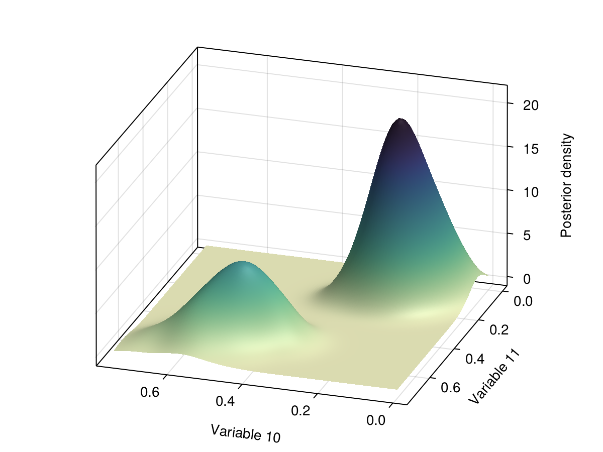
Figure 1.4: Visualization of the bridge SDE posterior distribution used to illustrate the various algorithms in this section. The SDE is a Wright–Fisher diffusion on $(0,1)$. Left: Distribution over SDE paths (red) bridging two fixed anchors and avoiding a hard constraint (thick black line). Middle: Pairwise distribution of variables in the neighborhood of the hard constraint showing multimodality. Right: Pair plot of all pairwise posterior distributions.

Running example

As a concrete running example in this section, consider the distribution over paths of a stochastic differential equation (SDE) bridging two fixed anchors while avoiding a hard constraint (see Fig. 1.4). In this setting, we take $X_{i}$ to be the random value at time point $i$ of the discretized process. In this example we use a discretization of the Wright–Fisher diffusion with Euler–Maruyama step-size $\delta$ [112], for which

$$X_{i}=G_{i}(X_{i-1},Z_{i})=\operatornamewithlimits{proj}_{[0,1]}\left(X_{i-1}+\mathchoice{{\hbox{$\displaystyle\sqrt{\delta X_{i-1}(1-X_{i-1})\,}$}\lower 0.4pt\hbox{\vrule height=7.5pt,depth=-6.00003pt}}}{{\hbox{$\textstyle\sqrt{\delta X_{i-1}(1-X_{i-1})\,}$}\lower 0.4pt\hbox{\vrule height=7.5pt,depth=-6.00003pt}}}{{\hbox{$\scriptstyle\sqrt{\delta X_{i-1}(1-X_{i-1})\,}$}\lower 0.4pt\hbox{\vrule height=5.25pt,depth=-4.20003pt}}}{{\hbox{$\scriptscriptstyle\sqrt{\delta X_{i-1}(1-X_{i-1})\,}$}\lower 0.4pt\hbox{\vrule height=3.75pt,depth=-3.00002pt}}}Z_{i}\right),$$ (1.90)

where $\operatornamewithlimits{proj}_{[0,1]}$ denotes a projection onto $[0,1]$ and $Z_{i}$ is standard normal. The Wright-Fisher diffusion model is used in population genetics to model the evolution of an allele frequency over time [124].

Sampling in $Z$-space

Because $X$ is a deterministic function of $Z$, one can define a sampler over either the $X$ variables (with prior denoted $\pi_{0}$) or the $Z$ variables (with prior denoted $f_{0}$). As we will see soon, in our example it is highly advantageous to define the chain on the variable $Z$, targeting the distribution

$$\tilde{\pi}(z)\propto f_{0}(z)\;L(G(z)),$$ (1.91)

where $f_{0}$ denotes the prior distribution on $Z$. Doing so will allow us to define a variational family that can be optimized using a simple moment matching algorithm. Morevoer, that algorithm achieves the fast convergence of second order methods without explictly forming a pre-conditioning matrix. Note that $\tilde{\pi}$ satisfies the property that the pushforward of $\tilde{\pi}$, denoted $\tilde{\pi}\circ G^{-1}$, is equal to $\pi$. In our running Wright-Fisher example, the reparameterized prior $f_{0}$ is a standard normal distribution.

Independence kernel Metropolis-Hastings algorithm

Consider one of the simplest possible sampling schemes: MCMC with an independence Metropolis-Hastings (IMH) kernel. In this section it will instead We use IMH as a pedagogical starting point leading to powerful MOI-based approximations for complex posterior distributions.

In IMH, the proposal $Z_{t}^{*}$ does not not depend on $Z_{t-1}$. Denote that proposal density by $f_{\phi}$. We first review the simple situation where $\phi$ is fixed, then extend to learning $\phi$ on the fly.

Recall the transition kernel of IMH is given by:

$$\addcontentsline{lla}{section}{\numberline{\string\crtrefnumber{eq:imh-kernel}}{e}q:imh-kernel}Z_{t}\leftarrow\operatorname{MH}_{\alpha_{\text{IMH}}}(Z_{t}^{*},Z_{t-1},U_{t}),\qquad Z_{t}^{*}\sim f_{\phi},\qquad\alpha_{\text{IMH}}(z^{*},z)=1\wedge\frac{\tilde{\pi}(z^{*})f_{\phi}(z)}{\tilde{\pi}(z)f_{\phi}(z^{*})},$$ (1.92)

where $U_{t}$ is i.i.d. uniform, and the MH kernel $\operatorname{MH}_{\alpha}(z^{*},z,u)$ is equal to $z^{*}$ if $u<\alpha$ and to $z$ otherwise.

The average rejection rate (RR) of the IMH algorithm at stationarity can be expressed in terms of the total variation distance. That is, for $Z\sim\tilde{\pi}$ and $Z^{*}\sim f_{\phi}$,

$$\addcontentsline{lla}{section}{\numberline{\string\crtrefnumber{eq:tv-bound}}{e}q:tv-bound}\text{RR}=1-\mathbb{E}[\alpha_{\text{IMH}}(Z^{*},Z)]=\mathrm{D_{TV}}(\tilde{\pi}\times f_{\phi},f_{\phi}\times\tilde{\pi})\leq 2\mathrm{D_{TV}}(\tilde{\pi},f_{\phi}).$$ (1.93)

We see from Eq. 1.93 that effective use of IMH relies on the construction of a proposal $f_{\phi}$ such that: (1) $f_{\phi}$ is close to $\tilde{\pi}$ in total variation distance; and (2) $f_{\phi}$ should be tractable, which we define in our context as being able to sample from $f_{\phi}$ i.i.d. and evaluate the density of $f_{\phi}$ pointwise.

With Eq. 1.93 in mind, the choice of the proposal distribution for an IMH algorithm can be cast as a minimization problem of the total variation distance between $\tilde{\pi}$ and a proposal distributions $f_{\phi}$.

Learning the independence kernel: formulation

We now formalize an optimization problem aimed at improving the IMH proposal. This example draws from the substantial literature on optimization of IMH proposals. Early work rooted in variational inference [32] is based on the reverse (exclusive) KL. The first implicit instance of forward (inclusive) KL optimization that we are aware of is in [43, Section 3], and the connection to forward KL optimization is made explicit in [5, Section 7]. See also [108] and [70] for further developments.

The space over which we are optimizing consists of a set of candidate proposal distributions, which we denote by ${\mathcal{F}}=\{f_{\phi}:\phi\in\Phi\}$. In our running example, we take ${\mathcal{F}}$ to be the set of multivariate normal distributions with diagonal covariance matrices. By construction, $f_{0}\in{\mathcal{F}}$, and hence optimization over ${\mathcal{F}}$ should not degrade performance compared to naive IMH based on the prior.

With greater generality, we may assume that ${\mathcal{F}}$ is an exponential family, which we construct in two steps: first defining $\bar{}{\mathcal{F}}$, then reindexing it to obtain ${\mathcal{F}}$. First, we define a canonical exponential family, $\bar{}{\mathcal{F}}=\{\bar{f}_{\eta}\}$,

$$\bar{f}_{\eta}(z)=\exp(\eta^{\top}s(z)-A(\eta)),$$ (1.94)

where $s$ is the sufficient statistic, $A$ is the log normalization function, and $\eta$ lies in some natural parameter space $E$. Second, letting $\sigma$ be the moment mapping,

$$\sigma(\eta):=\mathbb{E}[s(Z_{\eta})],\quad Z_{\eta}\sim\bar{f}_{\eta},$$ (1.95)

the exponential family ${\mathcal{F}}$ under the moment parameterization is given by

$${\mathcal{F}}=\{f_{\phi}:\phi\in\Phi\},\qquad f_{\phi}:=\bar{f}_{\sigma^{-1}(\phi)},\qquad\Phi:=\left\{\sigma(\eta):\eta\in E\right\}.$$ (1.96)

While Eq. 1.93 suggests an objective function based on the total variation distance, this objective is seldom directly used as an IMH tuning objective, with a few exceptions, e.g., [117, Appendix F.11.2]. Instead, the forward KL is often preferred [121, 62, 81] in the MCMC-driven optimization context. One motivation for this choice is its ease of optimization, as the forward KL minimization often admits closed-form updates. To see this, it is useful to recall the classical connection between forward KL minimization and maximum likelihood estimation. Let $\{Z_{t}\}_{t=1}^{T}$ denote MCMC samples with stationary distribution $\pi$. We have that

$$\operatornamewithlimits{arg\,min}_{\phi}\mathrm{D_{KL}}(\tilde{\pi}||f_{\phi})\approx\operatornamewithlimits{arg\,min}_{\phi}\frac{1}{T}\sum_{t=1}^{T}\log\frac{\tilde{\pi}(Z_{t})}{f_{\phi}(Z_{t})}=\operatornamewithlimits{arg\,max}_{\phi}\sum_{t=1}^{T}\log f_{\phi}(Z_{t}),$$ (1.97)

where we recognize in the final expression the maximum likelihood estimation objective function. We can therefore cast the problem of minimizing the forward KL as the following “artificial” statistical estimation problem: treat the samples $Z_{t}$ as observations, the family ${\mathcal{F}}$ as a statistical parametric model, and then perform maximum likelihood estimation from these observations.

Returning to our running example of a Wright-Fisher diffusion, where ${\mathcal{F}}$ consists of multivariate normal distributions with diagonal covariance matrices, we combine the above connection with the standard fact that the maximum likelihood under our Gaussian family has closed-form updates that consist of matching empirical first and second moments. To generalize this observation to other exponential families, note that, for $Z\sim\tilde{\pi}$,

$$\operatornamewithlimits{arg\,min}_{\eta}\mathrm{D_{KL}}(\tilde{\pi}||\bar{f}_{\eta}) =\operatornamewithlimits{arg\,max}_{\eta}\mathbb{E}[\log\bar{f}_{\eta}(Z)],$$ (1.98)

$$=\operatornamewithlimits{arg\,max}_{\eta}\eta^{\top}\mathbb{E}[s(Z)]-A(\eta).\addcontentsline{lla}{section}{\numberline{\string\crtrefnumber{kl-obj}}{k}l-obj}$$ (1.99)

Taking the gradient with respect to $\eta$, the critical points are given by

$$\mathbb{E}[s(Z)]-\nabla A(\eta)=0.$$ (1.100)

From basic exponential family properties, $\nabla A(\eta)=\mathbb{E}[s(Z_{\eta})]=\sigma(\eta)$. Hence, by exponential family convexity,

$$\operatornamewithlimits{arg\,min}_{\eta}\mathrm{D_{KL}}(\tilde{\pi}||\bar{f}_{\eta})=\sigma^{-1}(\mathbb{E}[s(Z)]).$$ (1.101)

In the moment parameterization, this is then simply

$$\addcontentsline{lla}{section}{\numberline{\string\crtrefnumber{eq:close-form}}{e}q:close-form}\operatornamewithlimits{arg\,min}_{\phi}\mathrm{D_{KL}}(\tilde{\pi}||f_{\phi})=\mathbb{E}[s(Z)].$$ (1.102)

In the following section we offer some practical advice for performing this optimization.

Learning the independence kernel: optimization

We present algorithms to perform the optimization formulated in the last section. In the following, let $Z_{1},Z_{2},\ldots$ be a sequence from a Markov chain and define

$$\bar{S}_{T}=\frac{1}{T}\sum_{t=1}^{T}S_{t},\qquad S_{t}=s\left(Z_{t}\right).$$ (1.103)

Suppose that $\mathbb{E}[\bar{S}_{T}]\overset{a.s.}{\to}s^{\star}=\mathbb{E}[s(Z)]$, where $Z\sim\tilde{\pi}$, as $T\to\infty$. In our context, because the $Z_{t}$ are Markovian, the convergence above is guaranteed by the law of large numbers for Markov chains. We also write $\bar{K}(\eta)=-\eta^{\top}s^{\star}+A(\eta)$ to denote our forward KL objective function under the natural parameterization, and $K(\phi)=\bar{K}(\sigma^{-1}(\phi))$ for the objective under the moment parameterization.

Naive stochastic gradient: because it is trivial to obtain stochastic gradients with respect to $\bar{K}$, it is tempting to use a simple SGD scheme of the form

$$\eta_{t}\leftarrow\eta_{t-1}-\gamma_{t}\hat{\nabla}_{t}\bar{K}(\eta_{t-1}),$$ (1.104)

where the deterministic and stochastic gradients are given by

$$\addcontentsline{lla}{section}{\numberline{\string\crtrefnumber{eq:gradient}}{e}q:gradient}\nabla\bar{K}(\eta)=-s^{\star}+\nabla A(\eta),\qquad\hat{\nabla}_{t}\bar{K}(\eta)=-S_{t}+\nabla A(\eta).$$ (1.105)

However, as we show below, in the present context this choice is strictly dominated in terms of performance and complexity of implementation by a simple moment-matching scheme [43, Section 3] that we present below.

From a pilot MCMC run: Consider a simplified setup where a pilot or warm-up MCMC run has produced estimates of the sufficient statistics parameter $\bar{S}_{t}$. In that case, working in the moment parameterization and using Eq. 1.102 yields the update $\phi\leftarrow\bar{S}_{t}$. While the moment parameterization $\phi$ is convenient for parameter estimation, it is often not directly supported by random number generator and density evaluation libraries, both of which are needed when proposing from the learned distribution $f_{\phi}$. This means that one has to convert $\phi$ into a more standard parameterization. In some cases, such as for normal distributions, this can be done in closed-form. In other cases, such as for gamma distributions, the moment mapping $\sigma(\eta)=\nabla A(\eta)$ might not have a closed-form inverse. When this is the case, one can use a “mini optimization” inner loop to compute $\sigma^{-1}$. The key point is that this mini-optimization has a compute cost independent of the number of samples $t$ and so it is not a bottleneck, especially since it can be warm-started at the previous point. This type of nested optimization is related to mirror descent [3].

Online method: Instead of doing a pilot MCMC run, one can instead continually update $\phi$ using an online mean estimator, such as

$$\addcontentsline{lla}{section}{\numberline{\string\crtrefnumber{eq:online}}{e}q:online}\phi_{t}\leftarrow\frac{(t-1)\phi_{t-1}+S_{t}}{t}=\phi_{t-1}+\frac{S_{t}-\phi_{t-1}}{t}.$$ (1.106)

This update can be seen as a special case of the online EM algorithm used in [5, Section 7.4] to learn an IMH sampler when setting the number of mixture components to one. We see in Fig. 1.5 that this online scheme strongly outperforms naive SGD. This might be surprising because the updates superficially appear very similar. We demystify this in Remark 1.5.2 by recasting the above moment update as a preconditioned SGD scheme.

Round-based method: In a distributed computational setting, an online update is less attractive as it produces diminishing changes per constant communication cost. Instead, one can use a round-based scheme (see [31] and [120, Section 5.4]), based on batches $\bar{S}^{(r)}$ where batch $r$ contains $2^{r}$ samples based on parameter $\phi^{(r)}=\bar{S}^{(r-1)}$.

Figure 1.5: Online learning of a normal distribution with mean $0.2$ and variance $0.4$ from i.i.d. draws.

Having presented several approaches to performing the optimization, we provide an end-to-end MOI algorithm example based on the developed methodology.

Example 1.5.1.

Denote the IMH kernel defined by Eq. 1.92 as $\kappa_{\phi}$. At each iteration $t$ we proceed as follows. First, we perform one IMH step using the current proposal parameter $\phi_{t-1}$ (Eq. 1.92 with $\phi=\phi_{t-1}$):

$$Z_{t}\sim\kappa_{\phi_{t-1}}(\cdot|Z_{t-1}).$$ (1.107)

Then, we compute the increment on the sufficient statistics, $S_{t}\leftarrow s(Z_{t})$, and update the proposal parameters via Eq. 1.106.

Remark 1.5.2.

To demystify the performance gap between naive SGD and moment matching that can be seen in Fig. 1.5, we review how Eq. 1.106 can be interpreted as SGD with a specific preconditioning matrix $P$ and learning rate sequence $\gamma_{t}$. For background on the closely related notion of a natural gradient, see [2]. Recall that pre-conditioned gradient descent of a function $H$ uses updates of the following form:

$$\addcontentsline{lla}{section}{\numberline{\string\crtrefnumber{eq:generic-newton}}{e}q:generic-newton}\phi_{t}\leftarrow\phi_{t-1}-\gamma_{t}P(\phi_{t-1})^{-1}\nabla H(\phi_{t-1}).$$ (1.108)

For example, Newton’s method uses the Hessian matrix as the pre-conditioner, so that $P(\phi)=\nabla^{2}H(\phi)$.

However, to make Eq. 1.108 coincide with moment matching, we have to use a different preconditioner than the Hessian matrix of the objective $H=K$ (recall that $K$ is the forward KL objective under the moment parameterization). To infer the preconditioner establishing the connection with moment matching, first note that by the chain rule,

$$\nabla K(\phi) =\nabla\{\bar{K}\circ\sigma^{-1}\}(\phi)$$ (1.109)

$$=\nabla\sigma^{-1}(\phi)^{\top}\nabla\{\bar{K}\}(\sigma^{-1}(\phi)).$$ (1.110)

Therefore, if we set $P=(\nabla\sigma^{-1})^{\top}$, we obtain

$$P(\phi)^{-1}\nabla K(\phi)=\nabla\{\bar{K}\}(\sigma^{-1}(\phi)).$$ (1.111)

Plugging this into Eq. 1.108 with $H=K$ and $P=(\nabla\sigma^{-1})^{\top}$, we obtain the update

$$\phi_{t}\leftarrow\phi_{t-1}-\gamma_{t}\nabla\{\bar{K}\}(\sigma^{-1}(\phi_{t-1})).$$ (1.112)

To conclude our connection to moment matching, we derive a stochastic version of the algorithm. From Eq. 1.105 and $\nabla A=\sigma$,

$$\hat{\nabla}_{t}\bar{K}(\sigma^{-1}(\phi_{t-1}))=-S_{t}+\phi_{t-1},$$ (1.113)

so setting $\gamma_{t}=1/t$, we obtain the moment matching update in Eq. 1.106.

To see that $P$ is distinct from the Hessian of the objective, it is enough to examine the univariate case:

$$K^{\prime}(\phi) =-(\sigma^{-1})^{\prime}(s^{\star}-\phi)$$ (1.114)

$$K^{\prime\prime}(\phi) =-(\sigma^{-1}(\phi))^{\prime\prime}(s^{\star}-\phi)+(\sigma^{-1}(\phi))^{\prime}$$ (1.115)

$$=P(\phi)-(\sigma^{-1}(\phi))^{\prime\prime}(s^{\star}-\phi).$$ (1.116)

Therefore, $P$ is close to the Hessian $K^{\prime\prime}$ when $\phi\approx s^{\star}$. This behaviour is seen empirically in Fig. 1.5: after a sufficient number of iterations, online moment matching is eventually indistinguishable from Hessian-conditioned natural gradient. The take-away message is that moment matching should be used whenever possible, given its ease of implementation and optimality properties [2, Section 4]. Both methods strongly outperform naive unconditioned SGD.

In Fig. 1.6 we present the improvements in effective sample size (ESS) per second when an optimized IMH kernel is used for the Wright–Fisher diffusion model at 20 discretized time points. We train the IMH kernel using the approach presented in Example 1.5.1, but with the round-based tuning procedure describe earlier. We alternate one iteration of IMH with one iteration of slice sampling, which performs well on targets with varying local geometry even with default settings.

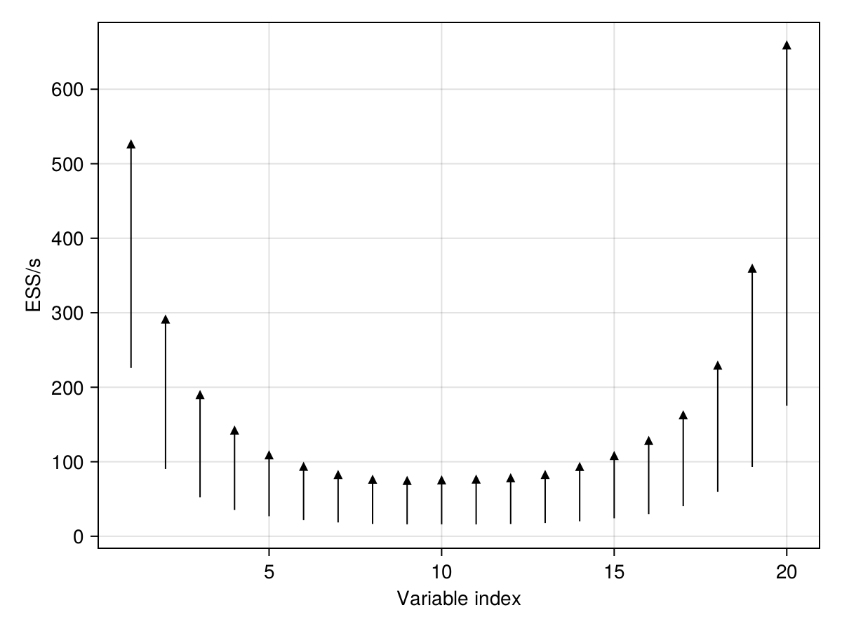
Figure 1.6: Improvement in ESS per second brought by the optimized IMH algorithm for the constrained Wright–Fisher diffusion. For each variable in the model (x-axis), we present the ESS per second (timings include variational training.). The baseline is a random walk MH algorithm (point at the beginning of each arrow), which we compare to an optimized IMH algorithm (point at the end of each arrow). Arrows pointing upwards represent an efficiency improvement brought by the optimized IMH kernel.

1.5.2 Scalability via tempering

We previously saw an example of an IMH kernel proposing from $q_{\phi}$ and targeting $\pi$. Such an approach tends to fail in high dimensions due to low MH acceptance probabilities as a consequence of the curse of dimensionality, which we illustrate below. One resolution to this problem is to bridge the gap between $q_{\phi}$ and $\pi$ by introducing a sequence of distributions lying on an annealing path between the two endpoints. We do so using a technique called parallel tempering. The hope is that MH acceptance probabilities between adjacent distributions on the path are higher and can help samples from $q_{\phi}$ travel to $\pi$. When only two distributions are used on the path, parallel tempering is actually equivalent to the IMH method from last section, but increasing the number of intermediate distributions in the path is key to high-dimensional scaling.

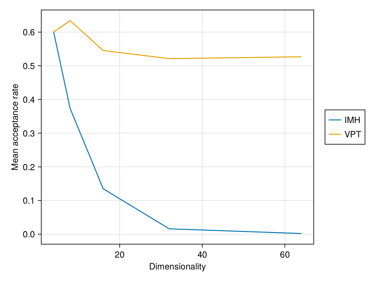
Figure 1.7: Left: Introduction of more “observations” (anchors) in the Wright–Fisher example. Here we show the distribution of paths obtained after adding one additional observation. Right: As more observations are introduced, the dimensionality of the posterior distribution increases, and the acceptance rate of the optimized IMH algorithm collapses exponentially fast (blue line). This is addressed by generalizing optimized IMH into a “variational parallel tempering” (VPT) algorithm. With VPT, a polynomial increase in the number of PT chains suffices to preserve a constant swap acceptance rate. Specifically, in this example we set the number of chains to $N\propto d^{1/2}$, as predicted in [11].

In the right panel of Fig. 1.7 we see that as the dimension of the problem increases, the IMH kernel acceptance probability approaches zero. To see that IMH proposals can result in very low acceptance probabilities in high dimensions, we consider the special case of product distributions. For $d\geq 1$, consider proposals from $q_{\phi}^{d}$ targeting $\pi^{d}$. Then, for $x_{0}^{d},x_{1}^{d}\in{\mathcal{X}}^{d}$, the corresponding IMH acceptance probability is given by

$$\alpha(d,x_{0}^{d},x_{1}^{d})=1\wedge\frac{\pi^{d}(x_{1}^{d})\cdot q_{\phi}^{d}(x_{0}^{d})}{\pi^{d}(x_{0}^{d})\cdot q_{\phi}^{d}(x_{1}^{d})}.$$ (1.117)

It can be shown that at stationarity—i.e., $X_{0}^{d}\sim\pi^{d}$ and $X_{1}^{d}\sim q_{\phi}^{d}$—for any $\epsilon>0$ we have

$$\alpha(d,X_{0}^{d},X_{1}^{d})^{d^{-1+\epsilon}}\xrightarrow{p}0,\qquad d\to\infty.$$ (1.118)

This suggests that the IMH acceptance probabilities decrease exponentially as the dimension of the problem increases and so IMH will generally not perform well in high dimensions without an annealing-based approach.

We demonstrate how to use tempering paths to obtain up to an exponential improvement for high-dimensional targets, as illustrated in the right panel of Fig. 1.7. One common path of distributions is given by

$$\addcontentsline{lla}{section}{\numberline{\string\crtrefnumber{eq:annealing_path}}{e}q:annealing_{p}ath}\pi_{\phi,\beta}=q_{\phi}^{1-\beta}\cdot\pi^{\beta},\qquad 0\leq\beta\leq 1.$$ (1.119)

This simple path, which linearly interpolates between log densities and uses a possibly tuned variational reference $q_{\phi}$ from which we can obtain i.i.d. samples, is one of many possible choices [117, 120]. This approach can also be seen as a generalization of some previous work on adaptive IMH proposals [32, 43, 70]. In the context of PT and annealing methods, this approach is similar to [20, Section 4.1] and [90, Section 5].

In the case of parallel tempering (PT), which we describe below, one can show that only $O(d)$ samples from $q_{\phi}^{d}$ are required to obtain an approximately independent sample from $\pi^{d}$ under appropriate assumptions [120, Theorems 1; Appendix F, Proposition 4], which is in stark contrast to the $O(c^{d})$ number of samples in the case of non-tempered IMH. There are several ways to take advantage of the annealing path in Eq. 1.119 to form an effective MCMC algorithm for sampling from $\pi$, including parallel tempering (PT) [45, 57, 119, 120] and simulated tempering methods [15, 46]. With both methods, a finite number of chains $N$ and an annealing schedule ${\mathcal{B}}_{N}=\{\beta_{n}\}_{n=0}^{N}$ with $0=\beta_{0}\leq\beta_{1}\leq\cdots\leq\beta_{N}=1$ are selected, which induce a sequence of distributions $\pi_{\phi,\beta_{n}}$ on the annealing path. Strategies for selecting the number of chains and an optimal annealing schedule exist in the literature on PT [120].

In PT, a Markov chain is constructed targeting $\pi_{\phi,\beta_{0}}\times\pi_{\phi,\beta_{1}}\times\cdots\times\pi_{\phi,\beta_{N}}$ on the augmented space ${\mathcal{X}}^{N+1}$. Updates on the augmented space proceed by alternating between two different types of Markov kernels referred to as local exploration and communication moves, respectively. For a given annealing parameter $\beta_{n}$, an exploration kernel $K^{(\beta_{n})}$ is assigned, such as a Hamiltonian Monte Carlo, Gibbs, or slice sampler. An exploration move consists of an application of each $K^{(\beta_{n})}$ to the $n^{\text{th}}$ marginal of the Markov chain. These updates are non-interacting and can be performed in parallel. However, the goal of tempering is to allow samples from the reference $q_{\phi}$ to travel to the target chain corresponding to $\pi$. This is achieved by allowing chains to interact using communication moves. These moves allow states between the $n^{\text{th}}$ and $(n+1)^{\text{th}}$ marginals of the Markov chain to be exchanged with a certain MH acceptance probability. We present pseudocode for non-reversible parallel tempering [120] in Algorithm 1. This approach to PT has been shown to provably dominate other PT approaches previously used in the literature [120].

Algorithm 1 Non-reversible parallel tempering

Initial state $\bar{x}_{0}\in{\mathcal{X}}^{N+1}$, annealing schedule $\mathcal{B}_{N}$, # iterations $T$, annealing path $\pi_{\beta}$ ($0\leq\beta\leq 1$)

for $t=1,2,\ldots,T$ do

    $\bar{x}\leftarrow\texttt{LocalExploration}(\bar{x}_{t-1},{\mathcal{B}}_{N},\pi_{\beta})$ $\triangleright$ Local exploration kernels

    $\triangleright$ $S_{\text{even}}$ and $S_{\text{odd}}$ are the even and odd subsets of $\{0,1,\ldots,N-1\}$

    if ($t-1$ is even) $S_{t}\leftarrow S_{\text{even}}$ else $S_{t}\leftarrow S_{\text{odd}}$

    for $n\in S_{t}$ do

        $\alpha\leftarrow 1\wedge\frac{\pi_{\beta_{n}}(x^{n+1})\cdot\pi_{\beta_{n+1}}(x^{n})}{\pi_{\beta_{n}}(x^{n})\cdot\pi_{\beta_{n+1}}(x^{n+1})}$

        $U\leftarrow\text{Unif}(0,1)$

        if $U\leq\alpha$ then $x^{n+1},\,x^{n}\leftarrow x^{n},\,x^{n+1}$ $\triangleright$ Swap components $n$ and $n+1$ of $\bar{x}$

    end for

    $\bar{x}_{t}\leftarrow\bar{x}$

end for

Return: $(\bar{x}_{t})_{t=0}^{T}$

It is preferable to parallelize computation because of the demands of working on the considerably larger augmented space ${\mathcal{X}}^{N+1}$. An efficient distributed implementation of PT in the Julia programming language is provided by [116]; this software is also used throughout this chapter to demonstrate several useful examples.

Stabilization

In our exposition of PT above, we introduced an annealing path between a variational reference $q_{\phi}$ and fixed target $\pi$, given by Eq. 1.119. This presentation has an added degree of freedom due to the ability to tune the reference; traditionally, a tempering path between a fixed reference $\pi_{0}$ and target $\pi$ is used. However, stable estimates of $\phi$ are necessary in this case: a locally (but not globally) optimal choice of $\phi$ can lead to poor samples that further reinforce our selection of $\phi$ in a non-global optimum. This issue is predicted by PT theory [117].

In the case of IMH, this issue can perhaps be seen even more clearly. If the IMH proposal from $q_{\phi}$ learns to only propose within one mode of a distribution, then we will see mode collapse: proposed samples will be from the given mode and it will be difficult to learn a better global proposal for $q_{\phi}$. In this case, one simple solution might be to alternate between the proposal $q_{\phi}$ and some fixed proposal $\pi_{0}$ to help avoid this issue of mode collapse.

To circumvent this issue in PT, it is necessary to stabilize PT when a variational reference $q_{\phi}$ is used. One solution is to introduce multiple reference distributions, by introducing multiple “legs” of PT [117]. For instance, one possible annealing path is

$$\pi_{\phi,\beta}\propto\begin{cases}q_{\phi}^{1-2\beta}\cdot\pi^{2\beta},&0\leq\beta\leq 0.5\\ \pi_{0}^{2\beta-1}\cdot\pi^{2-2\beta},&0.5<\beta\leq 1\\ \end{cases}$$ (1.120)

For more details about stabilizing PT using multiple reference distributions, we refer readers to [117].

1.5.3 Improving expressiveness using approximate transport

In this section we demonstrate one way of further increasing the expressiveness of $q_{\phi}$ using approximate transport maps. Transport-based methods construct a map, $f_{\phi}:{\mathcal{X}}\to{\mathcal{X}}$ for some $\phi\in\Phi$, such that the pushforward measure of some simple distribution $q$ with respect to $f_{\phi}$, denoted $q\circ f_{\phi}^{-1}$, is close to the target distribution $\pi$. In almost all cases $f_{\phi}$ is a diffeomorphism (both the map and its inverse are differentiable) for all $\phi$ so that the distribution of $q_{\phi}\equiv q\circ f_{\phi}^{-1}$ can be obtained by the change of variables formula. To find an $f_{\phi}$ such that $q_{\phi}$ is close to $\pi$, one typically minimizes $\mathrm{D_{KL}}(q_{\phi}||\pi)$. In the idealized setting, $q$ is a distribution from which we can obtain i.i.d. samples, such as a multivariate Gaussian, and hence minimization of the (reverse) KL divergence above can be achieved with gradient descent.

With the recent popularization of transport-based methods for inference such as normalizing flows (NFs) [34, 36, 88], a natural question that arises is whether these powerful methods can be applied to MCMC to assist MCMC exploration. Additionally, MCMC methods might be useful for minimizing other divergences such as the forward (inclusive) KL divergence $\mathrm{D_{KL}}(\pi||q_{\phi})$. A review of some advantages and drawbacks of methods that combine MCMC and normalizing flow methods is given by [50].

One approach, that we elaborate on in this section, is to (repeatedly) use a transport map from $q$ to $\pi$ and then use MCMC to sample from a distribution close to $\pi$ [10, 42, 54, 73, 111, 129]. We illustrate one example of such a method below, based on the work of [42]. We offer more details on other uses of approximate transport maps in conjunction with MCMC later in this section.

Given a transport map $f_{\phi}$ such that $q_{\phi}=q\circ f_{\phi}^{-1}\approx\pi$, and a $\pi$-invariant Markov kernel $\kappa$, we define the transport-based IMH kernel $\kappa_{T}$ as

$$\kappa_{T}(x,\mathrm{d}y;\phi) =\alpha(x,y)q_{\phi}(\mathrm{d}y)+(1-r(x))\delta_{x}(\mathrm{d}y)$$ (1.121)

$$r(x) =\int\alpha(x,y)q_{\phi}(\mathrm{d}y)$$ (1.122)

$$\alpha(x,y) =1\wedge\frac{\pi(y)q_{\phi}(x)}{\pi(x)q_{\phi}(y)}.$$ (1.123)

We can then compose $\kappa$ and $\kappa_{T}$ to obtain a composite kernel targeting $\pi$.

Following the work of [42], we update the parameters $\phi$ of the transport map as follows. The algorithm is presented in Algorithm 2. We start with $N$ particles, preferably initialized within each of the separate modes of the target distribution $\pi$. The states of these particles are denoted $\{x_{n}\}_{n=1}^{N}$. These particles are then separately updated using $a\geq 1$ applications of the $\pi$-invariant Markov kernel $\kappa$, followed by one application of the IMH transport map kernel $\kappa_{T}$. Along the way, obtained samples $\{x_{n}(k)\}_{n=1}^{N}$ for $k\geq 1$ are used to update the transport map $f_{\phi}$. Instead of minimizing the forward KL divergence $\mathrm{D_{KL}}(\pi||q_{\phi})$, which requires samples from the intractable target $\pi$, the approach taken in [42] is to minimize a KL divergence between $q_{\phi}\kappa^{k}$ and $q_{\phi}$. Specifically, at time step $k$, the loss for a given $\phi$ is proportional to $\mathrm{D_{KL}}(q_{\phi}\kappa^{k}||q_{\phi})$ and the estimate of the loss is given by

$${\mathcal{L}}_{N}(\phi)=-\frac{1}{N}\sum_{n=1}^{N}\log q_{\phi}(x_{n}(k)).$$ (1.124)

This loss is then minimized using gradient descent. The output of the algorithm is an approximating distribution $q_{\phi}$, as well as a collection of samples approximately distributed according to $\pi$, $\{x_{n}(k)\}_{k=0,n=1}^{k_{\text{max}},N}$.

Algorithm 2 Adaptive MC with transport maps [42]

target $\pi$, initial map $f_{\phi}$, starting particles $\{x_{n}(0)\}_{n=1}^{N}$, total duration $k_{\text{max}}$, number of applications of $\kappa$ before applying $f_{\phi}$: $a$, gradient step size $\epsilon$

for $k=0,2,\ldots,k_{\text{max}}-1$ do

    for $n=1,2,\ldots,N$ do

        if $k\text{ mod }a+1=0$ then

           $x_{n}(k+1)\sim\kappa_{T}(x_{n}(k),\cdot)$

        else

           $x_{n}(k+1)\sim\kappa(x_{n}(k),\cdot)$

        end if

    end for

    ${\mathcal{L}}_{N}(\phi)\leftarrow-\frac{1}{N}\sum_{n=1}^{N}\log q_{\phi}(x_{n}(k+1))$

    $\phi\leftarrow\phi-\epsilon\nabla_{\phi}{\mathcal{L}}_{N}(\phi)$

end for

Return: $\{x_{n}(k)\}_{k=0,n=1}^{k_{\text{max}},N},f_{\phi}$

Algorithm 2 can be connected to the variational PT algorithm presented in Section 1.5.2. In [42], the authors remark that the use of a fixed kernel $\kappa$ in conjunction with the adaptive $\kappa_{T}$ “improves the robustness of the scheme by ensuring that sampling proceeds in places within the modes where the map is not optimal,” which is similar to the variational PT stabilization procedure previously mentioned. However, referring to Algorithm 2, “one should not expect the procedure to find states in basins distinct from initialization” [42]. This is because the fixed kernel $\kappa$ will likely remain trapped within a given mode of initialization; such problems can be avoided with the use of annealing. There is therefore likely room for annealing-based methods to be used to improve Algorithm 2.

A note on approximate transport maps for pre-conditioning

An alternative method of combining MCMC and transport, compared to the method introduced above, is to construct a map $f_{\phi}$, sample from $\pi\circ f_{\phi}$ using MCMC, and then push forward the obtained samples through $f_{\phi}$ [19, 55, 72, 91]. The main premise is that $\pi\circ f_{\phi}$ should lie close to $q$, which is chosen to be a distribution that is easy to sample from. These methods may work well when both $q$ and $\pi$ are log-concave distributions, however if the distributions have a different structure (e.g., $\pi$ is multimodal), then it can be difficult to find an invertible transform $f_{\phi}$ that can capture this structure.

The use of such transport maps for the purposes of performing MCMC sampling on a simpler space was studied by [75, Section 2.4], [72] and [91]. For example, [72] consider a polynomial-based approach for $f_{\phi}$. However, this approach was noted by [55] to be too expensive when the target distribution lives in a high-dimensional space. To this end, [55] consider using inverse autoregressive flows (IAFs) and Hamiltonian Monte Carlo (HMC) on the $q$ space to improve the performance of the method. In a similar vein, [19] consider training a map $f_{\phi}$ to minimize $\mathrm{D_{KL}}(q\circ f_{\phi}^{-1}||\pi)$ where $q$ is chosen to be a multivariate normal distribution. Then, an elliptical slice sampler [80] is used to sample from $\pi\circ f_{\phi}$, which should be approximately normally distributed.

1.6 Discussion

In this chapter we presented a unifying framework for many problems at the intersection of MCMC and machine learning, which we refer to as Markovian optimization-integration (MOI) problems. These problems encompass black-box variational inference, adaptive MCMC, normalizing flow construction and transport-assisted MCMC, surrogate-likelihood MCMC, coreset construction for MCMC with big data, Markov chain gradient descent, Markovian score climbing, and more. By unifying these problems, theory and methods developed for each may be translated and generalized. After presenting a list of some common MOI problems, we presented an example with techniques for MCMC-driven distribution approximation, as well as some other common strategies for tackling MOI problems and some convergence theory.

Although the MOI framework is very general, there are still some optimization-integration problems that cannot be captured with this approach. For instance, it may be the case that the Markovian assumption presented is still too strong. To achieve an even greater level of generality, we may wish to substitute results for gradient estimates with Markovian noise with any estimators that are asymptotically consistent. However, as we discussed in Section 1.4, replacing an i.i.d. assumption with a Markovian noise assumption leads to a more complicated set of sufficient theoretical conditions that guarantee convergence; generalizing beyond a Markovian noise assumption could yield even greater difficulties for the study of theoretical convergence properties.

1.7 Further reading

1.7.1 In this book

Chapter 2 discusses the adaptive MCMC literature, which is complementary to the present chapter. In the setups explored in the chapter on adaptive MCMC, the optimized parameter $\phi^{\star}$ is in itself not of primary interest; for instance, $\phi$ may be a proposal bandwidth in that setting. In contrast, for the class of methods reviewed here, finding $\phi^{\star}$ is often a part of or even the whole objective. For instance, one may consider the case where $\phi$ parameterizes a rich parametric family approximating the posterior distribution.

Chapter 23 covers state-of-the-art methods to perform Bayesian inference over deep neural networks, while the methods explored in the present chapter are agnostic to the nature of the posterior distribution. Deep neural networks are often part of MCMC-driven learning methods, but focus so far has been on fitting them using non-Bayesian methods.

1.7.2 Other connections

“Big data” has been a major focus in both machine learning and statistics in the past 10 years. Section 1.2 reviews many important techniques used to approach large datasets, including black-box variational inference and coreset MCMC, both of which use as a building block the mini-batch gradient estimation reviewed in Section 1.3.3. However, this only scratches the surface of the range of methods developed to approach large datasets. See, for example, [9] for a review of other techniques such as data subsampling and divide-and-conquer MCMC methods.

While we have focused mostly on the machine learning, statistics and optimization literatures, MOI problems have been studied in many other fields. In particular, they arise in reinforcement learning and control under the name of “average reward problems” [69]. Even within a given field, it is often studied separately in different subfields. For example, in machine learning they are studied both in the optic of large-scale training (where gradient stochasticity is a purely algorithmic device) and in the sub-field of online learning (where the stochasiticity is viewed as epistemic) [26]. Similarly, due to space constraints we have skipped other important MOI applications, for example to Monte Carlo and stochastic EM [40, 110].

For simplicity, we have assumed throughout the chapter that the Markov kernel $\kappa_{\phi}$ is exactly $\pi_{\phi}$-invariant. However, there has been recently a resurgence of interest in methods where $\kappa_{\phi}$ is only approximately $\pi_{\phi}$-invariant [37, 126]. The most popular example comes from unadjusted approximations to Langevin dynamics [39, 84], often combined with stochastic gradients. These “unadjusted” methods typically have a worse asymptotic rate of convergence compared to exactly invariant kernels. Instead, unadjusted methods are typically advantageous in the initial “burn-in” phase [125], making them a good match with the MOI setup.

References

- [1] Alekh Agarwal, Peter L. Bartlett, Pradeep Ravikumar, and Martin J. Wainwright. Information-theoretic lower bounds on the oracle complexity of stochastic convex optimization. IEEE Transactions on Information Theory, 58(5):3235–3249, 2012.
- [2] Shun’ichi Amari. Natural gradient works efficiently in learning. Neural Computation, 10(2):251–276, 1998.
- [3] Ehsan Amid and Manfred K. Warmuth. Reparameterizing mirror descent as gradient descent. Advances in Neural Information Processing Systems, 33:8430–8439, 2020.
- [4] Christophe Andrieu, Éric Moulines, and Pierre Priouret. Stability of stochastic approximation under verifiable conditions. In IEEE Conference on Decision and Control, 2005.
- [5] Christophe Andrieu and Éric Moulines. On the ergodicity properties of some adaptive MCMC algorithms. The Annals of Applied Probability, 16(3):1462–1505, 2006.
- [6] Christophe Andrieu and Christian Robert. Controlled MCMC for optimal sampling. Cahiers du Cérémade 0125, 2001.
- [7] Christophe Andrieu and Johannes Thoms. A tutorial on adaptive MCMC. Statistics and Computing, 18:343–373, 2008.
- [8] Christophe Andrieu and Matti Vihola. Markovian stochastic approximation with expanding projections. Bernoulli, 20(2):545–585, 2014.
- [9] Elaine Angelino, Matthew James Johnson, Ryan P Adams, et al. Patterns of scalable Bayesian inference. Foundations and Trends in Machine Learning, 9(2-3):119–247, 2016.
- [10] Michael Arbel, Alex Matthews, and Arnaud Doucet. Annealed flow transport Monte Carlo. In International Conference on Machine Learning, pages 318–330. PMLR, 2021.
- [11] Yves F Atchadé, Gareth O Roberts, and Jeffrey S Rosenthal. Towards optimal scaling of Metropolis-coupled Markov chain Monte Carlo. Statistics and Computing, 21:555–568, 2011.
- [12] Atilim Gunes Baydin, Barak A Pearlmutter, Alexey Andreyevich Radul, and Jeffrey Mark Siskind. Automatic differentiation in machine learning: A survey. Journal of Machine Learning Research, 18:1–43, 2018.
- [13] Mark A Beaumont, Wenyang Zhang, and David J Balding. Approximate Bayesian computation in population genetics. Genetics, 162(4):2025–2035, 2002.
- [14] Albert Benveniste, Michel Métivier, and Pierre Priouret. Adaptive Algorithms and Stochastic Approximations, volume 22. Springer Science & Business Media, 2012.
- [15] Miguel Biron-Lattes, Trevor Campbell, and Alexandre Bouchard-Côté. Automatic regenerative simulation via non-reversible simulated tempering. arXiv:2309.05578, 2023.
- [16] David M Blei, Alp Kucukelbir, and Jon D McAuliffe. Variational inference: A review for statisticians. Journal of the American Statistical Association, 112(518):859–877, 2017.
- [17] Antoine Bordes, Léon Bottou, and Patrick Gallinari. SGD-QN: Careful quasi-Newton stochastic gradient descent. Journal of Machine Learning Research, 10(59):1737–1754, 2009.
- [18] James Bradbury, Roy Frostig, Peter Hawkins, Matthew James Johnson, Chris Leary, Dougal Maclaurin, George Necula, Adam Paszke, Jake VanderPlas, Skye Wanderman-Milne, and Qiao Zhang. JAX: Composable transformations of Python+NumPy programs, 2018.
- [19] Alberto Cabezas and Christopher Nemeth. Transport elliptical slice sampling. In Artificial Intelligence and Statistics, pages 3664–3676. PMLR, 2023.
- [20] Ewan Cameron and Anthony Pettitt. Recursive pathways to marginal likelihood estimation with prior-sensitivity analysis. Statistical Science, 29(3):397–419, 2014.
- [21] Trevor Campbell and Boyan Beronov. Sparse variational inference: Bayesian coresets from scratch. Advances in Neural Information Processing Systems, 32, 2019.
- [22] Trevor Campbell and Tamara Broderick. Bayesian coreset construction via greedy iterative geodesic ascent. In International Conference on Machine Learning, pages 698–706. PMLR, 2018.
- [23] Trevor Campbell and Tamara Broderick. Automated scalable Bayesian inference via Hilbert coresets. The Journal of Machine Learning Research, 20(1):551–588, 2019.
- [24] Yair Carmon and Oliver Hinder. Making SGD parameter-free. In Proceedings of Thirty Fifth Conference on Learning Theory, pages 2360–2389. PMLR, 2022.
- [25] George Casella and Christian P Robert. Rao-Blackwellisation of sampling schemes. Biometrika, 83(1):81–94, 1996.
- [26] Nicolò Cesa-Bianchi and Gábor Lugosi. Prediction, Learning, and Games. Cambridge University Press, Cambridge ; New York, 2006.
- [27] Han-Fu Chen, Lei Guo, and Ai-Jun Gao. Convergence and robustness of the Robbins–Monro algorithm truncated at randomly varying bounds. Stochastic Processes and their Applications, 27:217–231, 1988.
- [28] Han-Fu Chen and Yun-Min Zhu. Stochastic approximation procedures with randomly varying truncations. Scientia Sinica 1, 29:914–926, 1986.
- [29] Naitong Chen and Trevor Campbell. Coreset Markov chain Monte Carlo. arXiv:2310.17063, 2023.
- [30] Naitong Chen, Zuheng Xu, and Trevor Campbell. Bayesian inference via sparse Hamiltonian flows. Advances in Neural Information Processing Systems, 35:20876–20888, 2022.
- [31] Cyril Chimisov, Krzysztof Latuszynski, and Gareth Roberts. Air Markov chain Monte Carlo, 2018. arXiv:1801.09309.
- [32] Nando de Freitas, Pedro Højen-Sørensen, Michael I Jordan, and Stuart Russell. Variational MCMC. In Proceedings of the Seventeenth Conference on Uncertainty in Artificial Intelligence, pages 120–127, 2001.
- [33] Ron S. Dembo and Trond Steihaug. Truncated-Newton algorithms for large-scale unconstrained optimization. Mathematical Programming, 26(2):190–212, 1983.
- [34] Laurent Dinh, Jascha Sohl-Dickstein, and Samy Bengio. Density estimation using Real NVP. arXiv:1605.08803, 2016.
- [35] John Duchi, Elad Hazan, and Yoram Singer. Adaptive subgradient methods for online learning and stochastic optimization. Journal of Machine Learning Research, 12(7), 2011.
- [36] Conor Durkan, Artur Bekasov, Iain Murray, and George Papamakarios. Neural spline flows. Advances in Neural Information Processing Systems, 32, 2019.
- [37] Alain Durmus and Éric Moulines. High-dimensional Bayesian inference via the unadjusted Langevin algorithm. Bernoulli, 25(4A), 2019.
- [38] Alain Durmus, Éric Moulines, Alexey Naumov, and Sergey Samsonov. Finite-time High-probability Bounds for Polyak-Ruppert Averaged Iterates of Linear Stochastic Approximation, 2023. arXiv:2207.04475.
- [39] Donald L. Ermak. A computer simulation of charged particles in solution. The Journal of Chemical Physics, 62(10):4189–4196, 1975.
- [40] Gersende Fort and Éric Moulines. Convergence of the Monte Carlo expectation maximization for curved exponential families. The Annals of Statistics, 31(4):1220–1259, 2003.
- [41] Michael P. Friedlander and Mark Schmidt. Hybrid deterministic-stochastic methods for data fitting. SIAM Journal on Scientific Computing, 34(3):A1380–A1405, 2012.
- [42] Marylou Gabrié, Grant M Rotskoff, and Eric Vanden-Eijnden. Adaptive Monte Carlo augmented with normalizing flows. Proceedings of the National Academy of Sciences, 119(10):e2109420119, 2022.
- [43] Jørund Gåsemyr. On an adaptive version of the Metropolis–Hastings algorithm with independent proposal distribution. Scandinavian Journal of Statistics, 30(1):159–173, 2003.
- [44] Tomas Geffner and Justin Domke. MCMC variational inference via uncorrected Hamiltonian annealing. In Advances in Neural Information Processing Systems, 2021.
- [45] Charles J Geyer. Markov chain Monte Carlo maximum likelihood. Computing Science and Statistics, Proceedings of the 23rd Symposium on the Interface, pages 156–163, 1991.
- [46] Charles J Geyer and Elizabeth A Thompson. Annealing Markov chain Monte Carlo with applications to ancestral inference. Journal of the American Statistical Association, 90(431):909–920, 1995.
- [47] Saeed Ghadimi and Guanghui Lan. Stochastic first- and zeroth-order methods for nonconvex stochastic programming. SIAM Journal on Optimization, 23(4), 2013.
- [48] Peter W. Glynn. Likelihood ratio gradient estimation for stochastic systems. Communications of the ACM, 33(10):75–84, 1990.
- [49] Robert Gower, Mark Schmidt, Francis Bach, and Peter Richtárik. Variance-reduced methods for machine learning. Proceedings of the IEEE, 108(11):1968–1983, 2020.
- [50] Louis Grenioux, Alain Durmus, Éric Moulines, and Marylou Gabrié. On sampling with approximate transport maps. arXiv:2302.04763, 2023.
- [51] Tian-De Guo, Yan Liu, and Cong-Ying Han. An overview of stochastic quasi-Newton methods for large-scale machine learning. Journal of the Operations Research Society of China, 11(2):245–275, 2023.
- [52] Michael U Gutmann, Jukka Cor, et al. Bayesian optimization for likelihood-free inference of simulator-based statistical models. Journal of Machine Learning Research, 17(125):1–47, 2016.
- [53] Heiko Haario, Eero Saksman, and Joanna Tamminen. An adaptive Metropolis algorithm. Bernoulli, 7(2):223–242, 2001.
- [54] Paul Hagemann, Johannes Hertrich, and Gabriele Steidl. Stochastic normalizing flows for inverse problems: a Markov chains viewpoint. SIAM/ASA Journal on Uncertainty Quantification, 10(3):1162–1190, 2022.
- [55] Matthew Hoffman, Pavel Sountsov, Joshua V Dillon, Ian Langmore, Dustin Tran, and Srinivas Vasudevan. NeuTra-lizing bad geometry in Hamiltonian Monte Carlo using neural transport. arXiv:1903.03704, 2019.
- [56] Jonathan Huggins, Trevor Campbell, and Tamara Broderick. Coresets for scalable Bayesian logistic regression. Advances in Neural Information Processing Systems, 29, 2016.
- [57] Koji Hukushima and Koji Nemoto. Exchange Monte Carlo method and application to spin glass simulations. Journal of the Physical Society of Japan, 65(6):1604–1608, 1996.
- [58] Maor Ivgi, Oliver Hinder, and Yair Carmon. DoG is SGD’s best friend: A parameter-free dynamic step size schedule, 2023. arXiv:2302.12022.
- [59] Martin Jankowiak and Du Phan. Surrogate likelihoods for variational annealed importance sampling. arXiv:2112.12194, 2021.
- [60] Marko Järvenpää, Michael U Gutmann, Arijus Pleska, Aki Vehtari, and Pekka Marttinen. Efficient acquisition rules for model-based approximate Bayesian computation. Bayesian Analysis, 14(2):595–622, 2019.
- [61] Kirthevasan Kandasamy, Jeff Schneider, and Barnabás Póczos. Query efficient posterior estimation in scientific experiments via Bayesian active learning. Artificial Intelligence, 243:45–56, 2017.
- [62] Kyurae Kim, Jisu Oh, Jacob Gardner, Adji Bousso Dieng, and Hongseok Kim. Markov chain score ascent: A unifying framework of variational inference with Markovian gradients. Advances in Neural Information Processing Systems, 35:34802–34816, 2022.
- [63] Sujin Kim, Raghu Pasupathy, and Shane Henderson. A guide to sample average approximation. In Handbook of Simulation Optimization, volume 216, pages 207–243. Springer, 2015.
- [64] Diederik P. Kingma and Jimmy Ba. Adam: A method for stochastic optimization. In International Conference on Learning Representations, 2015.
- [65] Diederik P Kingma and Max Welling. Auto-encoding variational Bayes. In International Conference on Learning Representations, 2014.
- [66] Alp Kucukelbir, Dustin Tran, Rajesh Ranganath, Andrew Gelman, and David M Blei. Automatic differentiation variational inference. Journal of Machine Learning Research, 2017.
- [67] Yunwen Lei, Ting Hu, Guiying Li, and Ke Tang. Stochastic gradient descent for nonconvex learning without bounded gradient assumptions. IEEE Transactions on Neural Networks and Learning Systems, 31(10):4394–4400, 2020.
- [68] Dong C. Liu and Jorge Nocedal. On the limited memory BFGS method for large scale optimization. Mathematical Programming, 45(1):503–528, 1989.
- [69] Sridhar Mahadevan. Average reward reinforcement learning: Foundations, algorithms, and empirical results. Machine Learning, 22(1):159–195, 1996.
- [70] Florian Maire, Nial Friel, Antonietta Mira, and Adrian E. Raftery. Adaptive incremental mixture Markov chain Monte Carlo. Journal of Computational and Graphical Statistics, 28(4):790–805, 2019.
- [71] Dionysis Manousakas, Zuheng Xu, Cecilia Mascolo, and Trevor Campbell. Bayesian pseudocoresets. Advances in Neural Information Processing Systems, 33:14950–14960, 2020.
- [72] Youssef Marzouk, Tarek Moselhy, Matthew Parno, and Alessio Spantini. An introduction to sampling via measure transport. arXiv:1602.05023, 2016.
- [73] Alex Matthews, Michael Arbel, Danilo Jimenez Rezende, and Arnaud Doucet. Continual repeated annealed flow transport Monte Carlo. In International Conference on Machine Learning, pages 15196–15219. PMLR, 2022.
- [74] Edward Meeds and Max Welling. GPS-ABC: Gaussian process surrogate approximate Bayesian computation. In Uncertainty in Artificial Intelligence, pages 593–602, 2014.
- [75] Xiao-Li Meng and Stephen Schilling. Warp Bridge Sampling. Journal of Computational and Graphical Statistics, 11(3):552–586, 2002.
- [76] Shakir Mohamed, Mihaela Rosca, Michael Figurnov, and Andriy Mnih. Monte Carlo gradient estimation in machine learning. Journal of Machine Learning Research, 21(132):1–62, 2020.
- [77] Grégoire Montavon, Geneviève B. Orr, and Klaus-Robert Müller, editors. Neural Networks: Tricks of the Trade: Second Edition, volume 7700 of Lecture Notes in Computer Science. Springer Berlin Heidelberg, 2012.
- [78] Jacques Morgenstern. How to compute fast a function and all its derivatives: a variation on the theorem of Baur-Strassen. ACM SIGACT News, 16(4):60–62, 1985.
- [79] Éric Moulines and Francis Bach. Non-asymptotic analysis of stochastic approximation algorithms for machine learning. In Advances in Neural Information Processing Systems, volume 24, 2011.
- [80] Iain Murray, Ryan Adams, and David MacKay. Elliptical slice sampling. In International Conference on Artificial Intelligence and Statistics, pages 541–548. JMLR Workshop and Conference Proceedings, 2010.
- [81] Christian Naesseth, Fredrik Lindsten, and David Blei. Markovian score climbing: Variational inference with KL(p||q). Advances in Neural Information Processing Systems, 33:15499–15510, 2020.
- [82] Cian Naik, Judith Rousseau, and Trevor Campbell. Fast Bayesian coresets via subsampling and quasi-Newton refinement. Advances in Neural Information Processing Systems, 35:70–83, 2022.
- [83] Stephen G. Nash. A survey of truncated-Newton methods. Journal of Computational and Applied Mathematics, 124(1):45–59, 2000.
- [84] Radford Neal. Bayesian learning via stochastic dynamics. In Advances in Neural Information Processing Systems, volume 5, 1992.
- [85] A. Nemirovski, A. Juditsky, G. Lan, and A. Shapiro. Robust stochastic approximation approach to stochastic programming. SIAM Journal on Optimization, 19(4):1574–1609, January 2009.
- [86] A. S. Nemirovski and D. B. Yudin. Problem Complexity and Method Efficiency in Optimization. Wiley-Interscience Series in Discrete Mathematics. Wiley, Chichester ; New York, 1983.
- [87] Y. Nesterov. A method for solving the convex programming problem with convergence rate . Proceedings of the USSR Academy of Sciences, 1983.
- [88] George Papamakarios, Eric Nalisnick, Danilo Jimenez Rezende, Shakir Mohamed, and Balaji Lakshminarayanan. Normalizing flows for probabilistic modeling and inference. The Journal of Machine Learning Research, 22(1):2617–2680, 2021.
- [89] George Papamakarios, David Sterratt, and Iain Murray. Sequential neural likelihood: Fast likelihood-free inference with autoregressive flows. In Artificial Intelligence and Statistics, pages 837–848, 2019.
- [90] Ulrich Paquet, Ole Winther, and Manfred Opper. Perturbation corrections in approximate inference: Mixture modelling applications. Journal of Machine Learning Research, 10(43):1263–1304, 2009.
- [91] Matthew D Parno and Youssef M Marzouk. Transport map accelerated Markov chain Monte Carlo. SIAM/ASA Journal on Uncertainty Quantification, 6(2):645–682, 2018.
- [92] Boris Polyak. Some methods of speeding up the convergence of iteration methods. USSR Computational Mathematics and Mathematical Physics, 4(5):1–17, 1964.
- [93] Boris Polyak. New stochastic approximation type procedures. Avtomatica i Telemekhanika, 7:98–107, 1990.
- [94] Leah F Price, Christopher C Drovandi, Anthony Lee, and David J Nott. Bayesian synthetic likelihood. Journal of Computational and Graphical Statistics, 27(1):1–11, 2018.
- [95] Alexander Rakhlin, Ohad Shamir, and Karthik Sridharan. Making gradient descent optimal for strongly convex stochastic optimization. In International Conference on Machine Learning, 2012.
- [96] Rajesh Ranganath, Sean Gerrish, and David Blei. Black box variational inference. In Artificial Intelligence and Statistics, pages 814–822. PMLR, 2014.
- [97] Carl Rasmussen. Gaussian processes to speed up hybrid Monte Carlo for expensive Bayesian integrals. In Bayesian Statistics, pages 651–659, 2003.
- [98] Sashank J. Reddi, Satyen Kale, and Sanjiv Kumar. On the convergence of Adam and beyond. In International Conference on Learning Representations, 2018.
- [99] Sashank J Reddi, Satyen Kale, and Sanjiv Kumar. On the convergence of Adam and beyond. arXiv:1904.09237, 2019.
- [100] Danilo Rezende and Shakir Mohamed. Variational inference with normalizing flows. In International Conference on Machine Learning, 2015.
- [101] Danilo Jimenez Rezende, Shakir Mohamed, and Daan Wierstra. Stochastic backpropagation and approximate inference in deep generative models. In International Conference on Machine Learning, pages 1278–1286, 2014.
- [102] Herbert Robbins and Sutton Monro. A stochastic approximation method. Annals of Mathematical Statistics, 22(3):400–407, 1951.
- [103] Gareth O Roberts, Andrew Gelman, and Walter R Gilks. Weak convergence and optimal scaling of random walk Metropolis algorithms. The Annals of Applied Probability, 7(1):110–120, 1997.
- [104] Gareth O Roberts and Jeffrey S Rosenthal. Optimal scaling of discrete approximations to Langevin diffusions. Journal of the Royal Statistical Society: Series B (Statistical Methodology), 60(1):255–268, 1998.
- [105] Gareth O Roberts and Jeffrey S Rosenthal. Examples of adaptive MCMC. Journal of Computational and Graphical Statistics, 18(2):349–367, 2009.
- [106] Donald B Rubin. Bayesianly justifiable and relevant frequency calculations for the applied statistician. The Annals of Statistics, pages 1151–1172, 1984.
- [107] Reuven Y. Rubinstein. Sensitivity analysis of discrete event systems by the “push out” method. Annals of Operations Research, 39(1):229–250, 1992.
- [108] Håvard Rue, Ingelin Steinsland, and Sveinung Erland. Approximating hidden Gaussian Markov random fields. Journal of the Royal Statistical Society: Series B (Statistical Methodology), 66(4):877–892, 2004.
- [109] D. Ruppert. Efficient Estimations from a Slowly Convergent Robbins-Monro Process. Technical report, Cornell University Operations Research and Industrial Engineering, 1988.
- [110] William Ruth. A review of Monte Carlo-based versions of the EM algorithm, 2024. arXiv:2401.00945.
- [111] Sergey Samsonov, Evgeny Lagutin, Marylou Gabrié, Alain Durmus, Alexey Naumov, and Éric Moulines. Local-global MCMC kernels: The best of both worlds. Advances in Neural Information Processing Systems, 35:5178–5193, 2022.
- [112] Simo Särkkä and Arno Solin. Applied Stochastic Differential Equations, volume 10. Cambridge University Press, 2019.
- [113] Mark Schmidt, Nicolas Le Roux, and Francis Bach. Minimizing finite sums with the stochastic average gradient. Mathematical Programming, 162(1):83–112, 2017.
- [114] John Schulman, Sergey Levine, Pieter Abbeel, Michael Jordan, and Philipp Moritz. Trust region policy optimization. In International Conference on Machine Learning, pages 1889–1897. PMLR, 2015.
- [115] Tao Sun, Yuejiao Sun, and Wotao Yin. On Markov chain gradient descent. Advances in Neural Information Processing Systems, 31, 2018.
- [116] Nikola Surjanovic, Miguel Biron-Lattes, Paul Tiede, Saifuddin Syed, Trevor Campbell, and Alexandre Bouchard-Côté. Pigeons.jl: Distributed sampling from intractable distributions. arXiv:2308.09769, 2023.
- [117] Nikola Surjanovic, Saifuddin Syed, Alexandre Bouchard-Côté, and Trevor Campbell. Parallel tempering with a variational reference. Advances in Neural Information Processing Systems, 35:565–577, 2022.
- [118] Ilya Sutskever, James Martens, George Dahl, and Geoffrey Hinton. On the importance of initialization and momentum in deep learning. In International Conference on Machine Learning, pages 1139–1147, 2013.
- [119] Robert H Swendsen and Jian-Sheng Wang. Replica Monte Carlo simulation of spin-glasses. Physical Review Letters, 57(21):2607, 1986.
- [120] Saifuddin Syed, Alexandre Bouchard-Côté, George Deligiannidis, and Arnaud Doucet. Non-reversible parallel tempering: A scalable highly parallel MCMC scheme. Journal of the Royal Statistical Society: Series B (Statistical Methodology), 84(2):321–350, 2022.
- [121] Saifuddin Syed, Vittorio Romaniello, Trevor Campbell, and Alexandre Bouchard-Côté. Parallel tempering on optimized paths. In International Conference on Machine Learning, pages 10033–10042. PMLR, 2021.
- [122] Esteban Tabak and Cristina Turner. A family of nonparametric density estimation algorithms. Communications on Pure and Applied Mathematics, 66(2):145–164, 2013.
- [123] Esteban Tabak and Eric Vanden-Eijnden. Density estimation by dual ascent of the log-likelihood. Communications in Mathematical Sciences, 8(1):217–233, 2010.
- [124] Paula Tataru, Maria Simonsen, Thomas Bataillon, and Asger Hobolth. Statistical inference in the Wright–Fisher model using allele frequency data. Systematic Biology, 66(1):e30–e46, 2017.
- [125] YW Teh, A Thiery, and SJ Vollmer. Consistency and fluctuations for stochastic gradient Langevin dynamics. Journal of Machine Learning Research, 17(7):1–33, 2016. Publisher: Journal of Machine Learning Research.
- [126] Max Welling and Yee Whye Teh. Bayesian learning via stochastic gradient Langevin dynamics. In International Conference on Machine Learning, pages 681–688, 2011.
- [127] Richard Wilkinson. Accelerating ABC methods using Gaussian processes. In Artificial Intelligence and Statistics, pages 1015–1023, 2014.
- [128] Simon N Wood. Statistical inference for noisy nonlinear ecological dynamic systems. Nature, 466(7310):1102–1104, 2010.
- [129] Hao Wu, Jonas Köhler, and Frank Noé. Stochastic normalizing flows. Advances in Neural Information Processing Systems, 33:5933–5944, 2020.
- [130] Laurent Younes. On the convergence of Markovian stochastic algorithms with rapidly decreasing ergodicity rates. Stochastics and Stochastic Reports, 65:177–228, 1999.
- [131] Cheng Zhang, Judith Bütepage, Hedvig Kjellström, and Stephan Mandt. Advances in variational inference. IEEE Transactions on Pattern Analysis and Machine Intelligence, 41(8):2008–2026, 2018.
- [132] Guodong Zhang, Kyle Hsu, Jianing Li, Chelsea Finn, and Roger Grosse. Differentiable annealed importance sampling and the perils of gradient noise. In Advances in Neural Information Processing Systems, 2021.