Horseshoe Priors for Sparse Dirichlet-Multinomial Models

Abstract

Bayesian inference for Dirichlet-Multinomial (DM) models has a long and important history. The concentration parameter $\alpha$ is pivotal in smoothing category probabilities within the multinomial distribution and is crucial for the inference afterward. Due to the lack of a tractable form of its marginal likelihood, $\alpha$ is often chosen ad-hoc, or estimated using approximation algorithms. A constant $\alpha$ often leads to inadequate smoothing of probabilities, particularly for sparse compositional count datasets. In this paper, we introduce a novel class of prior distributions facilitating conjugate updating of the concentration parameter, allowing for full Bayesian inference for DM models. Our methodology is based on fast residue computation and admits closed-form posterior moments in specific scenarios. Additionally, our prior provides continuous shrinkage with its heavy tail and substantial mass around zero, ensuring adaptability to the sparsity or quasi-sparsity of the data. We demonstrate the usefulness of our approach on both simulated examples and on a real-world human microbiome dataset. Finally, we conclude with directions for future research.

Key Words: Hierarchical Modeling, Conjugate Bayesian Analysis, Dirichlet-Multinomial, Continuous Shrinkage Prior, Sparse Compositional Counts

1 Introduction

In this paper, we provide a conjugate family of prior distributions for full Bayesian inference for Dirichlet-Multinomial models. In particular, a horseshoe-type default prior is proposed for modeling high-dimensional quasi-sparse multinomial compositional count data with excessive zeros or values near zero. In real-world applications, zero-inflated count datasets are frequently encountered. For example, in bag-of-words analysis, certain words may exhibit frequent occurrences while others appear infrequently or not at all. Another example commonly discussed example is the human microbiome data (Zeng et al., 2022; Koslovsky, 2023), where structural zeros populate.

We first describe our setup for the Dirichlet-Multinomial (DM) distribution, denoted as ${\rm{DM}}({\bm{\alpha}},K,{\bm{n}})$. Let us consider $K$ categories with counts represented by ${\bm{n}}=(n_{1},\dots,n_{K})$, where the total count is $N=\sum_{k=1}^{K}n_{k}$. The model assumes that the vector of probabilities for each outcome, denoted by ${\bm{\pi}}=(\pi_{1},\pi_{2},...,\pi_{K})$, subjects to $\sum_{k=1}^{K}\pi_{k}=1$ and follows a Dirichlet distribution ${\rm{Dir}}({\bm{\alpha}})$ with hyperparameters ${\bm{\alpha}}=(\alpha_{1},\alpha_{2},\ldots,\alpha_{K})$. The Dirichlet density function is given by $p({\bm{\pi}}|{\bm{\alpha}})={{\mathcal{B}}({\bm{\alpha}})^{-1}}\prod_{k=1}^{K}\pi_{k}^{\alpha_{k}-1}$, where ${\mathcal{B}}({\bm{\alpha}})=\prod_{k=1}^{K}\Gamma(\alpha_{k})/\Gamma(A)$ with $A=\sum_{k=1}^{K}\alpha_{k}$ and $\Gamma(\cdot)$ is the Gamma function. The multinomial likelihood ${\rm{Mu}}({\bm{\pi}},{\bm{n}})$ for the count data is $p({\bm{n}}\mid{\bm{\pi}})={N!}/{(n_{1}!\cdots n_{K}!)}\times\prod_{k=1}^{K}\pi_{k}^{n_{k}}.$

One advantage of the Dirichlet prior is that the posterior of ${\bm{\pi}}$ also follows a Dirichlet distribution, given by

$$p({\bm{\pi}}\mid{\bm{n}},{\bm{\alpha}})=\frac{N!}{n_{1}!\cdots n_{K}!}\frac{1}{{\mathcal{B}}({\bm{\alpha}})}\prod_{k=1}^{K}\pi_{k}^{n_{k}+\alpha_{k}-1}\sim{\rm{Dir}}({\bm{n}}+{\bm{\alpha}}).$$ (1)

For simplicity of notation, we abuse the notation to denote the homogeneous Dirichlet distribution as ${\rm{Dir}}(\alpha)$, where $\alpha_{k}=\alpha$ for every $i={1,\ldots,K}$, and the corresponding DM distribution as ${\rm{DM}}(\alpha,K,{\bm{n}})$. The posterior mean from (1) has the form

$${\mathbb{E}}(\pi_{k}\mid{\bm{n}},{\bm{\alpha}})=\frac{n_{k}+\alpha_{k}}{N+\sum_{k=1}^{K}\alpha_{k}},$$ (2)

which corresponds to the probability estimator known as additive smoothing, Laplace smoothing or Lidstone smoothing (Lidstone, 1920). The conjugate nature of the Dirichlet distribution for the multinomial distribution and its ease of use have permitted good results in various modern applications, including Latent Dirichlet Allocation (LDA)(Blei et al., 2003), a popular topic modeling algorithm that is widely used in natural language processing.

Despite the prevalence of DM models, it has been a long-standing challenge to select its concentration hyperparameters ${\bm{\alpha}}$. The choice significantly impacts the posterior distribution of category probabilities and the model’s classification accuracy. Often the parameter is chosen in an ad-hoc manner, with common choices including the uniform prior $\alpha=1$, derived from first principles by Jeffreys (Jeffreys, 1939), and $\alpha=1/2$ according to Jeffreys’ rule (Jeffreys, 1946). Additionally, Perks (1947) proposed $\alpha=1/K$, recommended by Berger et al. (2015) as the “Overall Objective Prior”. Although additive smoothing is straightforward to implement, it can produce biased estimates and is not always effective in practice. Another approach to choosing ${\bm{\alpha}}$ is via maximum marginal likelihood $p({\bm{n}}\mid{\bm{\alpha}})$, also known as the empirical Bayes choice. However, $p({\bm{n}}\mid{\bm{\alpha}})$ is usually not analytically tractable. Various approximation schemes have been proposed to find the maximizer of the marginal distribution. The first type is to approximate the Dirichlet likelihood with a simpler function (Gamma density) by matching the first two derivatives (Minka, 2000). The same strategy was also used in inferring the Gamma shape parameter (Rossell, 2009; Miller, 2019). Another common strategy involves variants of the Expectation-Maximization (EM) algorithm, including Monte Carlo EM (Wallach, 2006) and variational EM (Blei et al., 2003). A different approach by George and Doss (2017) combines Markov Chain Monte Carlo (MCMC) and importance sampling to estimate the marginal likelihood up to a normalizing constant. Xia and Doss (2020) propose an MCMC-based fully Bayesian method to obtain the empirical Bayes estimate. However, these methods only provide a point estimate for $\alpha$ and are unable to supply uncertainty quantification. Liu et al. (2020) propose an empirical Bayes method by fixing $\alpha$ to the maximizer of the evidence, i.e., the marginal DM likelihood.

Another challenge arises from appropriately handling an abundance of zeros or small counts. The additive smoothing representation in (2) can bias inference. For example, for scenarios where $K>N$, many categories are expected to have zero counts, but the estimated probabilities for zero-count categories are strictly positive. Given the sparsity nature, an improperly chosen ${\bm{\alpha}}$ automatically reduces the probabilities of seen events to give a non-zero probability to non-seen events. This yields poor results for datasets with sparse or quasi-sparse counts. Alternatively, some models address the excess zeros with two-component zero-inflated priors, a technique that has also been seen in Poisson distributions (Lambert, 1992), negative binomial distributions (Yang et al., 2009), DM distributions (Koslovsky, 2023), generalized DM distributions (Tang and Chen, 2019), logistic normal Multinomial distributions (Zeng et al., 2022), and LDA models (Deek and Li, 2021). With the two-component mixtures, category probabilities $\pi_{k}$ can be directly set to zero with a non-zero probability. However, it is less flexible for quasi-sparse data, and the two-component mixture form likely leads to high computational costs.

In this paper, we propose a novel class of priors to address the challenges described above. By utilizing hierarchical modeling, we transfer the reference prior to a ‘higher level’ of the model, where we can impose desired structures on the model. First, our prior admits conjugate posterior computation for the DM distribution. By utilizing partial fraction decomposition, we are able to provide closed-form posterior moments for homogeneous cases. An extension of the class also allows for marginal posterior inference on the concentration parameter, $\alpha$, enabling high dimensional marginalization of the class probabilities. Second, our prior provides continuous shrinkage and adapts to the degree of sparsity or quasi-sparsity in the data. The shape of the prior is inspired by local-global shrinkage priors used in sparse Gaussian means and linear regression (Carvalho et al., 2010; Armagan et al., 2011, 2013; Bhattacharya et al., 2015), as well as quasi-sparse count data (Datta and Dunson, 2016). Our prior is also related to the Stirling-Gamma prior proposed in the independent work of Zito et al. (2023). Our prior places substantial mass around zero and possesses a heavy tail, allowing concentration parameters ${\bm{\alpha}}$ to move freely between zero and infinity.

The rest of the paper is outlined as follows. Section 2 provides the motivation for our priors and we introduce two classes of partial fraction priors tailored for DM models. Section 3 provides calculations for marginal posteriors and posterior moments, where we utilize recursive calculation of residues of the partial fraction representation of the posterior. We illustrate the efficacy of our proposed priors on simulated examples in Section 4 and validate the performance via real data analysis, focusing on microbiome studies, in Section 5. Finally, Section 6 wraps up with avenues for future research.

2 Conjugate Priors for Compositional Count Data

In this section, we first describe the motivation of how we construct a prior class that facilitates conjugate updating of the concentration parameter ${\bm{\alpha}}$. Later we delve into the selection of hyperparameters of this prior class. We show that with specific configurations, the prior exhibits two crucial properties essential for continuous sparsity-inducing regularization: (1) substantial mass around zero, and (2) a heavy tail. Essentially, we offer “a one-group answer to the two-groups problem” (Polson and Scott, 2010) for analyzing compositional count data.

2.1 Motivation

Our goal is to provide a flexible class of priors such that the marginal posterior inference for ${\bm{\alpha}}$ is computationally straightforward. We begin by examining the posterior in (1). One advantage of employing the Dirichlet prior is that we can marginalize out ${\bm{\pi}}$ to obtain a marginal likelihood for ${\bm{\alpha}}$ given the counts as

$$p({\bm{n}}\mid{\bm{\alpha}})=\frac{N!}{n_{1}!\cdots n_{K}!}\frac{B({\bm{n}}+{\bm{\alpha}})}{{\mathcal{B}}({\bm{\alpha}})}=\frac{N!}{\prod_{k}n_{k}!}\frac{\Gamma(\sum_{k}\alpha_{k})}{\prod_{k}\Gamma(\alpha_{k})}\frac{\prod_{k}\Gamma(n_{k}+\alpha_{k})}{\Gamma(N+\sum_{k}\alpha_{k})}=\frac{N!}{\prod_{k}n_{k}!}\frac{1}{[A]^{N}}\prod_{k}[\alpha_{k}]^{n_{k}}$$

where $[x]^{n}:=x(x+1)\cdots(x+n-1)$ is the rising Pochhammer polynomial. Thus, for any prior $p({\bm{\alpha}})$, by Bayes’ rule, we obtain the marginal posterior as

$$p({\bm{\alpha}}\mid{\bm{n}})\propto p({\bm{n}}\mid{\bm{\alpha}})p({\bm{\alpha}})\propto\frac{1}{[A]^{N}}\prod_{k}[\alpha_{k}]^{n_{k}}\times p({\bm{\alpha}}).$$

For simplicity, we first look into the homogeneous case where $\alpha_{k}=\alpha$, leading to $A=K\alpha$ and the posterior

$$p(\alpha\mid{\bm{n}})=\frac{1}{C_{N}}\frac{\prod_{k=1}^{K}[\alpha]^{n_{k}}}{[K\alpha]^{N}}p(\alpha).$$ (3)

where $C_{N}$ is a normalizing constant.

To construct a conjugate prior for the concentration parameter $\alpha$, we rewrite the fraction term as the sum of residuals (the explicit form of $\gamma_{i}$ will be introduced later) as

$$\frac{\prod_{k=1}^{K}[\alpha]^{n_{k}}}{[K\alpha]^{N}}=\sum_{i=1}^{N}\frac{\gamma_{i}\alpha}{K\alpha+i-1}.$$ (4)

Our objective now is to select a prior $p(\alpha)$ such that the following integral is in closed form

$$c_{i}=\int_{0}^{\infty}\frac{\alpha p(\alpha)}{K\alpha+i-1}{\mathrm{d}}\alpha.$$ (5)

Combining (4) and (5), the normalizing constant in (3), also known as the marginal belief, is

$$C_{N}=\int_{0}^{\infty}\frac{\prod_{k=1}^{K}[\alpha]^{n_{k}}}{[K\alpha]^{N}}p(\alpha){\mathrm{d}}\alpha=\sum_{i=1}^{N}\gamma_{i}c_{i}.$$ (6)

Motivated by the residual representation of Pochhammer polynomial ratios in (3), we introduce the Pochhammer prior family, such that (4) and (5) can be satisfied, while also allows for straightforward computation of posterior moments and predictive inference.

2.2 Pochhammer Priors

We define the Pochhammer distribution as follows.

Definition 1 (Pochhammer Distribution).

A random variable follows a Pochhammer distribution ${\rm{PH}}(\alpha|m,a,b,c)$ if its density function satisfies the following form

$$p(\alpha\mid m,a,b,c)\propto\frac{[\alpha]^{m}}{[c\alpha+a]^{b}}\,\text{ with }\alpha\geq 0$$

where $m,b$ are non-negative integers with $m\geq 0,b\geq m+2$, and $a>0,c>0$.

We impose the condition $b\geq m+2$ to ensure the integrability of the density function. To compute the normalizing constant for the Pochhammer distribution, we exploit the rational function nature of the ratio is a rational function and its partial fraction expansion representation.

Theorem 1.

If a random variable $\alpha\sim{\rm{PH}}(\alpha\mid m,a,b,c)$, its density function can be written explicitly as

$$p(\alpha\mid m,a,b,c)=C_{(m,a,b,c)}^{-1}\sum_{i=1}^{b}\frac{\gamma^{(m,a,b,c)}_{i}}{c\alpha+a+i-1}$$

where

$$\gamma^{(m,a,b,c)}_{i}=\left\{\begin{array}[]{cc}\frac{\prod_{s=1}^{m}(1+(s-1)c-a-i)}{c^{m}\prod_{k=1,\;k\neq i}^{b}(k-i)},&m\neq 0\\ \frac{1}{\prod_{k=1,\;k\neq i}^{b}(k-i)},&m=0\end{array}\right.\;\;C_{(m,a,b,c)}=\sum_{i=1}^{b}\frac{\big{(}-\gamma^{(m,a,b,c)}_{i}\big{)}}{c}\ln(a+i-1)$$

Proof.

For brevity, let $\gamma_{i}$ represent $\gamma^{(m,a,b,c)}_{i}$ in the proof. The partial fraction expansion for the ratio of Pochhammer polynomials is given by

$$\frac{[\alpha]^{m}}{[c\alpha+a]^{b}}=\sum_{i=1}^{b}\frac{\gamma_{i}}{c\alpha+a+i-1}\,\text{ where}\;\;\alpha\geq 0.$$

Here $\gamma_{i}$ are residues and are determined by solving a set of linear equations in Töeplitz form using Levinson’s algorithm. Specifically, the residues $\gamma_{i}$ can be calculated by carefully evaluating certain points of the identity (when $m\neq 0$)

$$\prod_{s=1}^{m}(\alpha+s-1)=\sum_{i=1}^{b}\gamma_{i}\prod_{k=1,\;k\neq i}^{b}(c\alpha+a+k-1).$$ (7)

If we evaluate at the points $\alpha=-(a+i-1)/c$, we get

$$\gamma_{j}=\frac{\prod_{s=1}^{m}(1+(s-1)c-a-i)}{c^{m}\prod_{k=1,\;k\neq i}^{b}(k-i)}.$$

This allows us to compute the normalizing constant as

$$C_{(m,a,b,c)} =\sum_{i=1}^{b}\int_{0}^{\infty}\frac{\gamma_{i}}{c\alpha+a+i-1}{\mathrm{d}}\alpha$$

$$=\sum_{i=1}^{b}\frac{\gamma_{i}}{c}\ln(c\alpha+a+i-1)\Big{\lvert}_{0}^{\infty}=-\sum_{i=1}^{b}\frac{\gamma_{i}}{c}\ln(a+i-1),$$

which follows from term-by-term integration and the key property of the residuals that $\sum_{i=1}^{b}\gamma_{i}=0$, and

$$\prod_{i=1}^{b}(c\alpha+a+i-1)^{\gamma_{i}}\rightarrow 1\;{\rm and}\;\sum_{i=1}^{b}(\gamma_{i}/c)\ln(c\alpha+a+i-1)\rightarrow 0\;\;{\rm as}\;\;\alpha\rightarrow\infty.$$

When $m=0$, the RHS of (7) is just $1$, the rest of the calculations follows through. ∎

The residual approach utilized here establishes a connection with the residual calculation techniques outlined in Barndorff-Nielsen et al. (1982, Lemma 3.1), which are commonly used in Pólya-Gamma and Pólya-Inverse-Gamma data augmentation (Polson et al., 2013; He et al., 2019).

2.3 Power Pochhammer Priors

The partial fraction class can be extended by size-biasing. We define the Power Pochhammer distribution as follows.

Definition 2 (Power Pochhammer Distribution).

A random variable $\alpha$ follows a Power Pochhammer distribution ${\rm{PPH}}(\alpha\mid m,a,b,c,d)$ if its density function satisfies the following form

$$p(\alpha\mid m,a,b,c,d)\propto\alpha^{d}\frac{[\alpha]^{m}}{[c\alpha+a]^{b}}\;\;{\rm with}\;\;\alpha\geq 0$$

where $b,d$ and $m$ are non-negative integers with $b\geq m+d+2$, and $a>0,c>0$.

Apparently, the Pochhammer distribution is a special case of Power Pochhammer distribution when $d=1$. Similar to Theorem 1, we can derive the explicit form for the density function of the Power Pochhammer distribution.

Theorem 2.

If a random variable $\alpha\sim{\rm{PPH}}(\alpha\mid m,a,b,c,d)$, then its density function can be written explicitly as

$$p(\alpha\mid m,a,b,c,d)=C_{(m,a,b,c,d)}^{-1}\sum_{i=1}^{b}\frac{\gamma^{(m,a,b,c,d)}_{i}}{c\alpha+a+i-1}$$ (8)

where

$$\gamma^{(m,a,b,c,d)}_{i}=\left\{\begin{array}[]{cc}\frac{(1-a-i)^{d}\prod_{s=1}^{m}(1+(s-1)c-a-i)}{c^{m+d}\prod_{k=1,\;k\neq i}^{b}(k-i)},&m>0\\ \frac{(1-a-i)^{d}}{c^{d}\prod_{k=1,\;k\neq i}^{b}(k-i)},&m=0\end{array}\right.\;\;C_{(m,a,b,c,d)}=\sum_{i=1}^{b}\frac{(-\gamma^{(m,a,b,c,d)}_{i})}{c}\ln(a+i-1)$$

Proof of this theorem is analogous to the proof provided for Theorem 1 and can be found in Section A.1.

Corollary 1 (Moments of Power Pochhammer distributions).

The distribution ${\rm{PPH}}(m,a,b,c,d)$ has up to $b-(m+d+2)$ moments. When $k\leq b-(m+d+2)$, Theorem 2 can also be used to calculate the $k$-th moments of a Power Pochhammer variable ${\rm{PPH}}(m,a,b,c,d)$ as

$${\mathbb{E}}(\alpha^{k})=\int\alpha^{k}p(\alpha\mid m,a,b,c,d){\mathrm{d}}\alpha=\frac{C_{(m,a,b,c,d+k)}}{C_{(m,a,b,c,d)}}\int p(\alpha\mid m,a,b,c,d+k){\mathrm{d}}\alpha=\frac{C_{(m,a,b,c,d+k)}}{C_{(m,a,b,c,d)}}$$

This identity also assists the calculation of posterior means and variances for probabilities, ${\bm{\pi}}$, in the count model via the law of iterated expectations, namely ${\mathbb{E}}({\bm{\pi}}\mid{\bm{n}})={\mathbb{E}}_{\alpha\mid{\bm{n}}}{\mathbb{E}}\big{(}{\bm{\pi}}\mid\alpha,{\bm{n}}\big{)}$ where the inner term ${\mathbb{E}}({\bm{\pi}}\mid\alpha,{\bm{n}})$ is calculated as (2).

2.4 Horseshoe-shape Priors

From the definition of the Pochhammer distribution, parameters $m$ and $b$ significantly influence the shape of the distribution, determining the available moments. Specifically, the parameter $m$ shapes of the distribution near $0$, with the prior having a non-diminishing mass around $0$ only if $m=0$. Parameter $b$ controls how heavy the right tail is.

For a desired continuous shrinkage prior that places a non-decaying mass around zero and possesses a heavy tail (Polson and Scott, 2010), we recommend the configuration of $m=0,b=2$. Under this configuration, the density function can be rewritten as

$$p(\alpha\mid m=0,a,b=2,c)\propto\frac{1}{(c\alpha+a)(c\alpha+a+1)}\propto\bigg{(}\frac{1}{\alpha+\frac{a}{c}}-\frac{1}{\alpha+\frac{a+1}{c}}\bigg{)}.$$

When $a$ is small and $c$ is large, we get a prior that is approximately

$$p(\alpha)\propto\bigg{(}\frac{1}{\alpha+\epsilon_{1}}-\frac{1}{\alpha+\epsilon_{1}+\epsilon_{2}}\bigg{)}$$

where both $\epsilon_{1}=\frac{a}{c}$ and $\epsilon_{2}=\frac{1}{c}$ are very small. This is the “closest to non-integrable” (on ${\mathbb{R}}^{+}$) fraction prior, exhibiting behavior similar to a horseshoe prior (Carvalho et al., 2010). It concentrates mass near $\alpha=0$, while its fat right tail allows the posterior to explore large values as well. As the distribution is supported on ${\mathbb{R}}^{+}$, we refer to the Pochhammer prior with $m=0$ as the “Half-Horseshoe” prior.

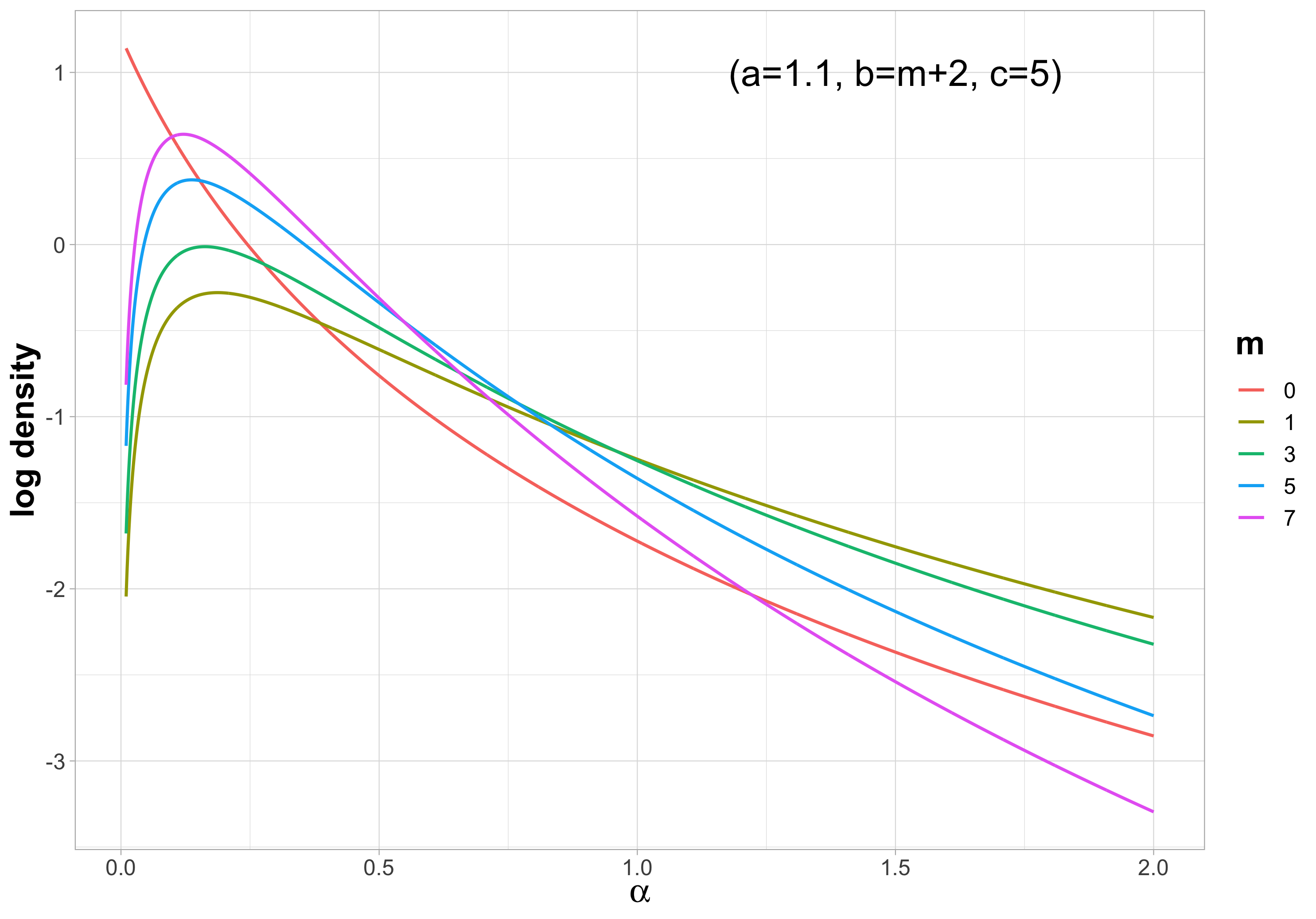
(a) $m$

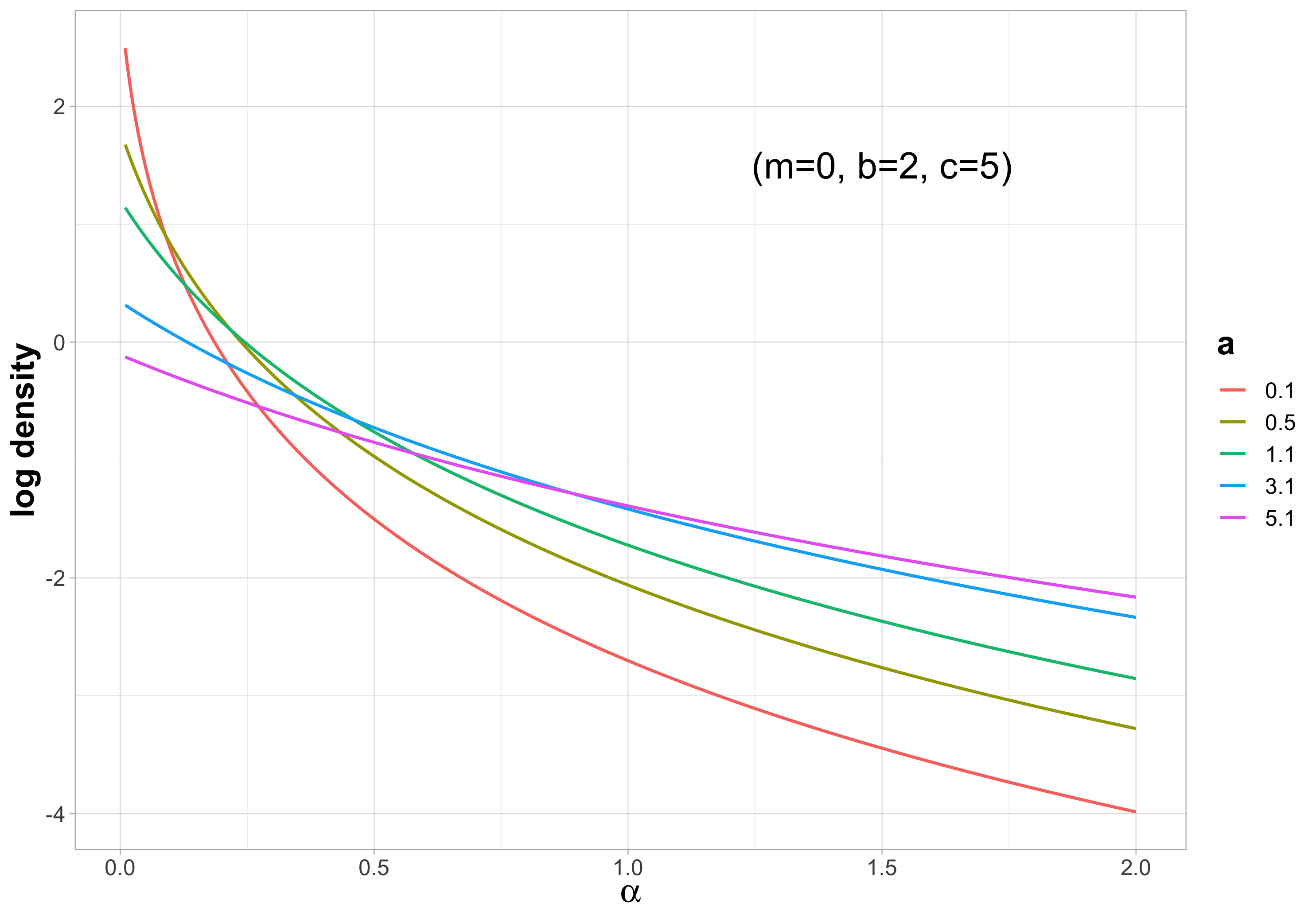
(b) $a$

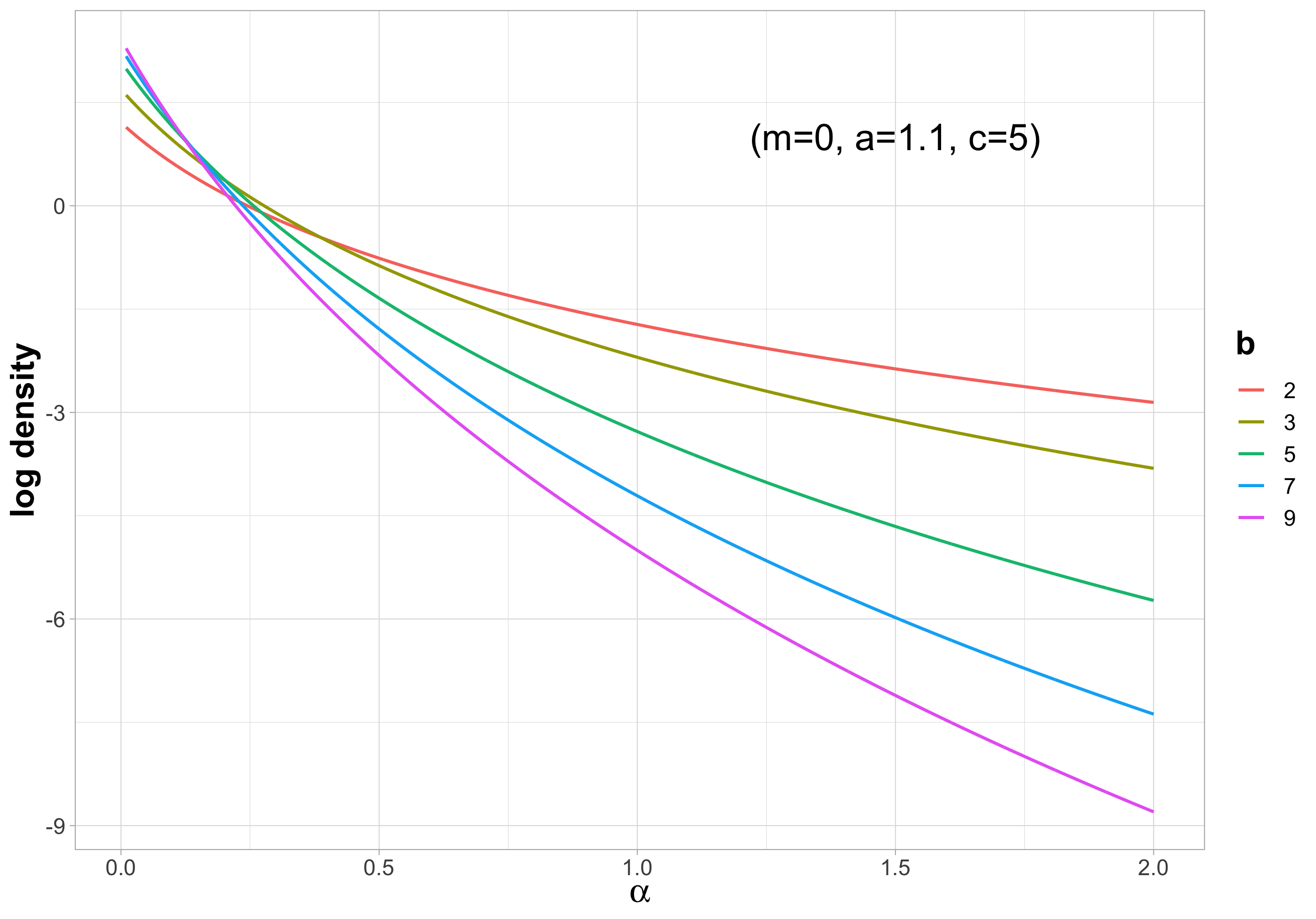
(c) $b$

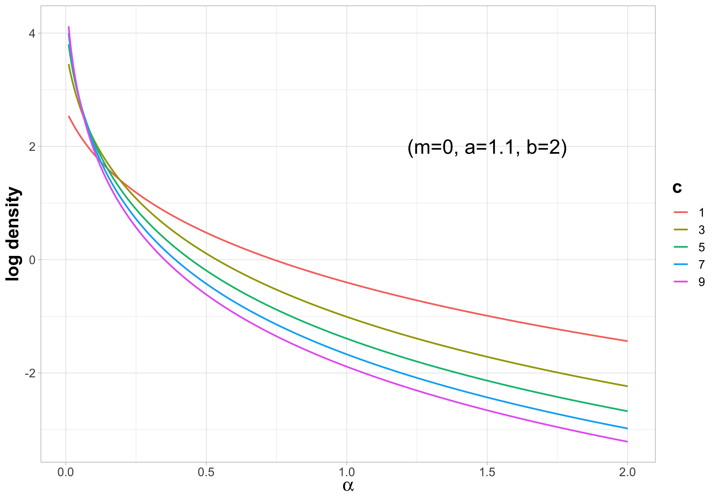
(d) $c$

Figure 1: Impact of hyperparameters on the shape of the Pochhammer distribution, shown in log scale. The baseline choice is $(m=0,a=1.1,c=5)$.

We provide intuitions on choosing hyperparameters for the Pochhammer prior in Figure 1. The baseline choice is $(m=0,a=1.1,b=2,c=5)$, and we examine the sensitivity of the prior’s shape to changes in each parameter. The most significant impact comes from $m$: when $m>0$, the prior immediately places zero mass at 0, losing the horseshoe shape. When $m\neq 0$, the tail becomes lighter when $m$ increases. When $m=0$, the tail is lighter with decreasing $a$, increasing $b$, or increasing $c$. Parameter $b$ determines the number of moments the prior and posterior distributions have. It requires $b\geq m+2$ for the density to be integrable on ${\mathbb{R}}^{+}$, and both the prior and posterior distributions have up to $(b-m-2)$ moments. We find that our posterior performance in the simulated examples in Section 4 is not very sensitive to the choices of $a$ and $c$, therefore, we proceed with $a=1$ and $c=1$.

Next, we verify the theoretical properties of our prior: heavy-tailed (Proposition 1) and super-efficient sparsity recovery (Proposition 2).

Proposition 1 (Heavy Tail).

The Pochhammer distribution $\alpha\sim{\rm{PH}}(m,a,b,c)$ exhibits heavy-tailed behavior, namely

$$\lim_{x\to\infty}e^{tx}P(\alpha>x)=\infty\quad\text{ for all }t>0.$$

Proof.

We utilize Stirling’s approximation of the Gamma function and the identity $\lim_{x\to\infty}(1+x/b)^{x}=e^{b}$. We have

$$\frac{1}{[cx+a]^{b}}=\frac{\Gamma(cx+a)}{\Gamma(cx+a+b)}\sim\frac{e^{-cx-a}(cx+a)^{cx+a-1/2}}{e^{-cx-a-b}(cx+a+b)^{cx+a+b-1/2}}\sim\frac{1}{(cx+a+b)^{b}},\quad x\to\infty.$$

Then we have

$$\frac{x^{m}}{[cx+a]^{b}}\sim\frac{x^{m}}{(cx+a+b)^{b}}\sim\frac{1}{c^{b}x^{b-m}},\quad x\to\infty,$$

since $b\geq m+2$ by definition. Combing the equations above with L’Hôpital’s rule, we can write

$$\lim_{x\to\infty}e^{tx}P(\alpha>x) =\lim_{x\to\infty}\frac{1}{C_{(m,a,b,c)}}\frac{\int_{x}^{\infty}\frac{\alpha^{m}}{[c\alpha+a]^{b}}{\mathrm{d}}\alpha}{e^{-tx}}$$

$$=\lim_{x\to\infty}\frac{1}{C_{(m,a,b,c)}}\frac{\frac{x^{m}}{[cx+a]^{b}}}{te^{-tx}}=\lim_{x\to\infty}\frac{1}{C_{(m,a,b,c)}}\frac{e^{tx}}{tc^{b}x^{b-m}}=\infty.$$

∎

Proposition 2 (Kullback-Leibler Risk Bounds from Polson and Scott (2010)).

Let $A_{\epsilon}=\{{\bm{\alpha}}:L(p_{{\bm{\alpha}}_{0}},p_{{\bm{\alpha}}})\leq\epsilon\}\in{\mathbb{R}}$ denote the Kullback-Leibler information neighborhood of size $\epsilon$, centered at ${\bm{\alpha}}_{0}$. Let $\mu_{N}({\mathrm{d}}{\bm{\alpha}})$ be the posterior distribution under $p({\bm{\alpha}})$ after observing the N counts data ${\bm{n}}=(n_{1},n_{2},\ldots,n_{K})^{\prime}$, and let $\hat{p}_{N}=\int p_{\bm{\alpha}}\mu_{N}({\mathrm{d}}{\bm{\alpha}})$ be the posterior mean estimator of the density function.

Suppose that the prior $p(\alpha)$ places positive mass in the neighborhood around $p_{{\bm{\alpha}}_{0}}$, i.e., $\mu(A_{\epsilon})>0$ for all $\epsilon>0$. Then the following bound for $R_{N}$, the Cesàro-average risk of the Bayes estimator $\hat{p}_{N}$, holds for all $\epsilon>0$:

$$R_{N}=\frac{1}{N}\sum_{j=1}^{N}L(p_{{\bm{\alpha}}_{0}},\hat{p}_{j})\leq\epsilon-\frac{1}{N}\log\int_{{\bm{\alpha}}-\sqrt{\epsilon}}^{{\bm{\alpha}}-\sqrt{\epsilon}}\pi({\bm{\alpha}}){\mathrm{d}}{\bm{\alpha}}.$$

Intuitively the more mass the prior $\pi({\bm{\alpha}})$ has in a neighborhood near the true value ${\bm{\alpha}}_{0}$, the better the bound is. Specifically, for the special case where $\alpha_{k}=0$ for some $k$, the risk bound can be greatly improved if the prior density has a pole at zero.

For our half-horseshoe Pochhammer prior, for example, ${\rm{PH}}(m=0,a=1,b=2,c=1)$, we have

$$\int_{0}^{\sqrt{\epsilon}}p(\alpha){\mathrm{d}}\alpha =\frac{1}{\log 2}\int_{0}^{\sqrt{\epsilon}}\frac{1}{(\alpha+1)(\alpha+2)}{\mathrm{d}}\alpha=\frac{1}{\log 2}\Big{[}\log(\alpha+1){\Big{|}}_{0}^{\sqrt{\epsilon}}-\log(\alpha+2){\Big{|}}_{0}^{\sqrt{\epsilon}}\Big{]}$$

$$=\frac{1}{\log 2}\log(1+\frac{\sqrt{\epsilon}}{2+\sqrt{\epsilon}})\approx\frac{1}{\log 2}\times\frac{\sqrt{\epsilon}}{2+\sqrt{\epsilon}}=o(\sqrt{\epsilon})\text{ when }\epsilon\to 0.$$

Thus the prior mass in the neighborhood is of order $\sqrt{\epsilon}$, which enables fast recovery of the true sampling distribution in sparse situations. This is one example of a KL “super efficient” prior.

In addition to the two properties above, we show that the limiting distribution when $b\to\infty$ is the exponential distribution ${\rm{Exp}}(1)$.

Proposition 3 (Limiting Distribution When $b\to\infty$).

Let $\alpha\sim{\rm{PH}}(m=0,a=1,b,c=1)$, then the following convergence in distribution holds:

$$\alpha\log b\to\gamma,\qquad\gamma\sim{\rm{Exp}}(1),\quad b\to\infty$$

Proof.

Plugging in the parameters we have

$$p(\alpha)\propto\frac{1}{[\alpha+1]^{b}}=\frac{\alpha}{[\alpha]^{b+1}},$$

which is equivalent to a Stirling-Gamma ${\rm{Sg}}(2,1,b)$ distribution. Using Proposition 1 of Zito et al. (2023), the limiting distribution of $\alpha\log b$ as $b\to\infty$ should be the Gamma distribution ${\rm Ga}(1,1)$, which is ${\rm{Exp}}(1)$. ∎

The proposition also implies that $\alpha\to 0$ in probability as $b\to\infty$ with a logarithmic rate of convergence via Slutzky’s theorem. We include a comparison between two distributions ${\rm{PH}}(m=0,a=1,b,c=1)$ and ${\rm Ga}(1,\log b)$ in Figure 2. While the two distributions look more similar as $b$ increases, it is worth noting that the Pochhammer distribution is heavy-tailed, with a larger mass near zero and a heavier right tail compared to the Gamma distribution.

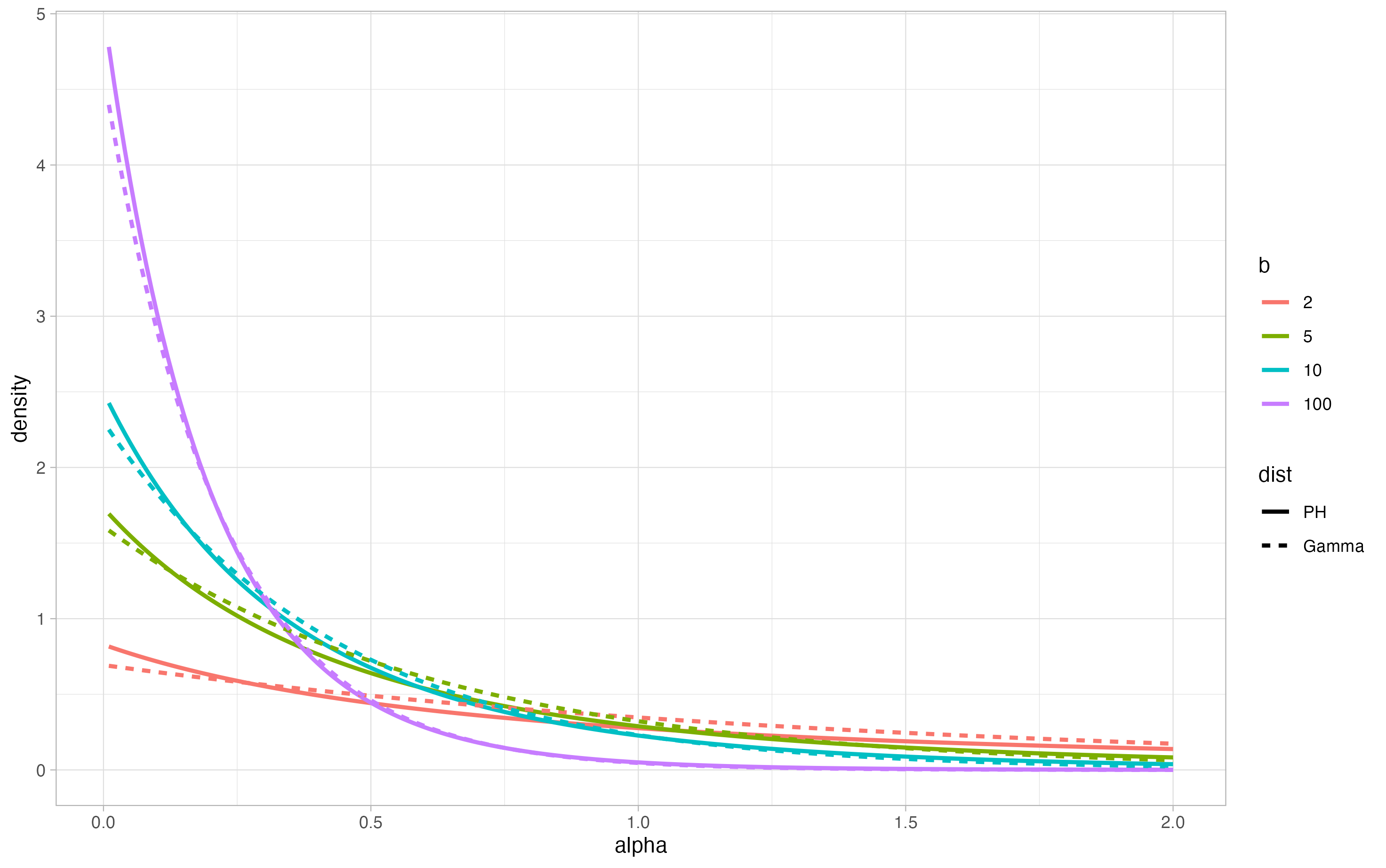
Figure 2: Comparison of density functions of ${\rm{PH}}(m=0,a=1,b,c=1)$ distribution and ${\rm Ga}(1,\log b)$ distribution.

Remark 1 (Connection to Zito et al. (2023)).

The Stirling-Gamma distributions proposed by Zito et al. (2023) have a similar form as our Pochhammer distributions and serve as a conjugate prior for the Dirichlet process. Despite the similar formula, our motivation and application are drastically different from theirs. We aim to propose a continuous shrinkage prior for sparse or quasi-sparse compositional count datasets, while Zito et al. (2023) focus on learning the number of clusters in the mixture models. Furthermore, the numerator of our marginal likelihood $p({\bm{n}}\mid{\bm{\alpha}})$ contains a product of Pochhammer polynomials, while the marginal likelihood of partitions $p(\Pi_{n}=\{C_{1},\ldots,C_{k}\}\mid\alpha)$ has powers of $\alpha$ in the numerator, which makes their posterior analysis more accessible than ours.

3 Full Bayesian Inference for DM models

In this section, we show how one can conduct full Bayesian inference for DM models in (1) under Pochhammer priors.

3.1 Posterior distribution for Homogeneous $\alpha$

When $\alpha_{k}$ is homogeneous, i.e., $\alpha_{k}=\alpha$ for every $k=1,\ldots,K$, closed-form representations for its posterior density and moments can be derived. We present one such case below. The dependence of the residual terms $\gamma_{i}^{*},\beta_{i}^{*}$ on $({\bm{n}},m,a,b,c)$ is removed for notational simplicity.

Theorem 3.

Under a Pochhammer prior $\alpha\sim{\rm{PH}}(m=n_{0},a,b,c)$, when there are no multiple roots in $[K\alpha]^{n}[c\alpha+a]^{b}$, the posterior in (3) has a closed-form representation as follows

$$p(\alpha\mid{\bm{n}})=C_{{\bm{n}}}(m,a,b,c)^{-1}\frac{\prod_{k=0}^{K}[\alpha]^{n_{k}}}{[K\alpha]^{N}[c\alpha+a]^{b}}=C_{{\bm{n}}}(m,a,b,c)^{-1}\left[\sum_{i=2}^{N}\frac{\gamma_{i}^{*}}{K\alpha+i-1}+\sum_{i=1}^{b}\frac{\beta_{i}^{*}}{c\alpha+a+i-1}\right]$$ (9)

where

$$\gamma_{i}^{*} =\frac{\prod_{k=0}^{K}\prod_{s=1}^{n_{k}}(1+(s-1)K-i)}{K^{N+n_{0}-b}\prod_{s=1,\;s\neq i}^{N}(s-i)\prod_{t=1}^{b}(Ka+K(t-1)-c(i-1))},$$

$$\beta_{i}^{*} =\frac{\prod_{k=0}^{K}\prod_{s=1}^{n_{k}}(1+(s-1)c-a-i)}{c^{n_{0}}\prod_{s=1}^{N}\big{(}K+c(s-1)-K(a+i)\big{)}\prod_{t=1,\;t\neq i}^{b}(t-i)},$$

$$C_{{\bm{n}}}(m,a,b,c) =\sum_{i=2}^{N}\frac{(-\gamma_{i}^{*})}{K}\ln(i-1)+\sum_{i=1}^{b}\frac{(-\beta_{i}^{*})}{c}\ln(a+i-1).$$

Proof.

The calculation follows from the same residual argument in Theorem 1.

Remark 2 (Multiple roots).

We choose to illustrate the simplest case where no multiple roots exist in the denominator. In practice, this requires some selection of parameters $a$ and $c$ to avoid the multiple roots. We provide an example in Section A.2 to show how the closed form representation can be derived when double roots are present. A more general recipe can be found in Zito et al. (2023).

Similar to Corollary 1, the posterior means ${\mathbb{E}}(\pi_{k}\mid{\bm{n}})$ and ${\mathbb{E}}\left(\alpha\mid{\bm{n}}\right)$ can be calculated using a residue argument.

Corollary 2 (Posterior Mean).

When $b\geq m+2$, by the law of iterated expectation, we can calculate the posterior means of the category probabilities, ${\pi}_{k},1\leq k\leq K$, via

$${\mathbb{E}}\left(\pi_{k}\mid{\bm{n}}\right)={\mathbb{E}}_{\alpha\mid{\bm{n}}}{\mathbb{E}}\left(\pi_{k}|\alpha,{\bm{n}}\right)={\mathbb{E}}_{\alpha\mid{\bm{n}}}\left(\frac{n_{k}+\alpha}{N+K\alpha}\right)$$

Under a Pochhammer prior ${\rm{PH}}(n_{0},a,b,c)$, we can write

$${\mathbb{E}}_{\alpha\mid{\bm{n}}}\left(\frac{n_{i}+\alpha}{N+K\alpha}\right) =\frac{1}{C_{{\bm{n}}}(n_{0},a,b,c)}\int_{0}^{\infty}\left(\frac{n_{i}+\alpha}{N+K\alpha}\right)\frac{\prod_{i=0}^{K}[\alpha]^{n_{k}}}{[K\alpha]^{N}[c\alpha+a]^{b}}\;{\mathrm{d}}\alpha=\frac{C_{{\bm{n}}+e_{k}}(n_{0},a,b,c)}{C_{{\bm{n}}}(n_{0},a,b,c)}$$

where $e_{i}=(0,\ldots,0,1,0,\ldots,0)^{\prime}$ is a vector that only the i-th element is 1 and zeros otherwise and

$$\left(\frac{n_{j}+\alpha}{N+K\alpha}\right)\frac{\prod_{i=0}^{K}[\alpha]^{n_{i}}}{[K\alpha]^{N}}=\frac{\prod_{i=0}^{K}[\alpha]^{n_{j,i}^{*}}}{[K\alpha]^{N+1}[K\alpha+a]^{b}},$$

such that $n_{j,i}^{*}=n_{i}$ for $j\neq i$ and $n_{i,i}^{*}=n_{i}+1$.

When $b=m+2$, we can calculate the expectation of the category probabilities ${\mathbb{E}}(\pi_{k}\mid{\bm{n}})$ but the expectation ${\mathbb{E}}(\alpha\mid{\bm{n}})$ does not exist. When $b\geq m+3$, the posterior mean for the concentration parameter $\alpha$ under the prior ${\rm{PH}}(m,a,b,c)$ is simply

$${\mathbb{E}}(\alpha\mid{\bm{n}})=\frac{C_{{\bm{n}}}(m+1,a,b,c)}{C_{{\bm{n}}}(m,a,b,c)}$$

3.2 Posterior Inference for Heterogeneous $\alpha_{k}$

While homogeneous DM models combined with PH priors enjoy closed-form representations, they are less flexible in adapting to the sparsity patterns in datasets. When the abundance of counts varies across different categories, it is more favorable to use heterogeneous DM models $DM({\bm{\alpha}},K,{\bm{n}})$.

We choose to use the same Pochhammer prior ${\rm{PH}}(\alpha_{k}\mid m,a,b,c)$ for each $\alpha_{k},k=1,\ldots,K$, aiming to treat all $\pi_{k}$ and $\alpha_{k}$ equally when no external information is available. Then the posterior in (3) is written as

$$p({\bm{\alpha}}\mid{\bm{n}})\propto\frac{1}{[A]^{N}}\prod_{k=1}^{K}\frac{[\alpha_{k}]^{n_{k}}[\alpha_{k}]^{m}}{[c\alpha_{k}+a]^{b}}$$ (10)

where $A=\sum_{k=1}^{K}\alpha_{k}$.

With $[A]^{N}$ in the denominator, the normalizing constant for the joint posterior in (10) is not straightforward to compute. Another observation is that given $A$, $\{\alpha_{k}\}_{k=1}^{K}$ are independent of each other. We can thus write the conditional posterior distribution of $\alpha_{k}$ as

$$p(\alpha_{k}\mid{\bm{n}},A_{-k})\propto\frac{1}{[\alpha_{k}+A_{-k}]^{N}}\frac{[\alpha_{k}]^{n_{k}}[\alpha_{k}]^{m}}{[c\alpha_{k}+a]^{b}}.$$ (11)

We employ Metropolis-Within-Gibbs sampling to obtain draws from the posterior, as outlined in Algorithm 1.

Remark 3 (Shrinking Posterior For Zero Counts).

Under a shrinkage prior ${\rm{PH}}(m=0,a,b,c)$, if the count $n_{k}=0$, the posterior in (11) can be simplified as

$$p(\alpha_{k}\mid{\bm{n}},A_{-k})\propto\frac{1}{[\alpha_{k}+A_{-k}]^{N}}\frac{1}{[c\alpha_{k}+a]^{b}}.$$

Given $A_{-k}>0$, the posterior distribution of $\alpha_{k}$ retains a horseshoe shape again. The posterior density has substantial mass around zero and is decreasing with respect to $\alpha_{k}$, which is desirable for analyzing sparse count datasets.

A major difference between our method and the zero-inflated models lies in how we model zero probabilities. While the zero-inflated DM models (Koslovsky, 2023) directly assign non-zero probabilities to events $\pi_{k}=0$, our approach allows the concentration parameter $\alpha_{k}\to 0$, resulting in the posterior of $\pi_{k}$ also places non-zero mass near zero. Thus our method offers “a one-group answer to a two-groups problem” in zero-inflated models. Additionally, retaining the concentration parameter ${\bm{\alpha}}$ in the hierarchical model is essential for model interpretation in many analyses.

Algorithm 1 Posterior Sampling When $\alpha_{k}$ is heterogeneous.

Input
Hyperparameters $m,a,b,c$, count data ${\bm{n}}$, stepsize $\sigma$
Sampling
Initialize parameters $\alpha_{k}^{(0)}\overset{\text{iid}}{\sim}\text{logNormal}(0,1)$ for $k=1,\ldots,K$
Metroplis-Within-Gibbs
For $t=1,\dots,T$:
For $k=1\ldots,K$:
Compute $A_{-k}=A-\alpha_{k}^{(t-1)}$
Propose $\alpha_{k}^{(t+1)}=\exp(\log(\alpha_{k}^{(t-1)})+\epsilon)$ with $\epsilon\sim{\mathcal{N}}(0,\sigma^{2})$
Compute log acceptance ratio $\text{LAR}=\log p(\alpha_{k}^{(t)}\mid{\bm{n}},A_{-k})-\log p(\alpha_{k}^{(t-1)}\mid{\bm{n}},A_{-k})$
Generate $u\sim\text{Unif}[0,1]$
If $\log(u)<\text{LAR}$, set $\alpha_{k}^{(t)}=\alpha_{k}^{(t-1)}$, else $A=A+\alpha_{k}^{(t)}-\alpha_{k}^{(t-1)}$
Return ${\bm{\alpha}}^{(1)},\ldots,{\bm{\alpha}}^{(T)}$

4 Simulations

We compare our methods with the following approaches: (1) A Bayesian DM model; (2) Tuyl’s approach Tuyl (2018); (3) A zero-inflated DM (ZIDM) model by Koslovsky (2023), where a latent variable is used to allow for exact zero probabilities. For each method, we obtain posterior draws from 10 000 MCMC iterations. We report the average absolute value of the difference between the estimated and true probabilities $\text{ABS}(\pi)=n^{-1}{\mathbb{E}}\|\hat{\pi}-\pi\|_{1}$ and 95% coverage probabilities (COV). We compute the statistics from 20 replicated datasets for each setting.

For our method, we consider both homogeneous (PH-h) and heterogeneous (PH-d) versions. To investigate how sensitive the posterior is to the shape of the prior distribution, we fix $a=c=1$ and include 4 configurations of parameters: (1) $m=0,b=2$; (2) $m=0,b=5$; (3) $m=1,b=3$; (4) $m=1,b=5$. We denote different configurations with subscripts. The posterior draws are also obtained from 10 000 MCMC iterations.

4.1 Scenario 1: A Single Document

We first consider the case of a single document and the number of categories $K$ is greater than the total counts $N$. We set $K=100$ and $N=50$. We examine four different settings here and the results are reported in Table 1. The first two settings are generated with fix ${\bm{\pi}}$ and the latter two are generated with fix ${\bm{\alpha}}$.

MTD	DM	Tuyl	ZIDM	PH1-h	PH2-h	PH3-h	PH4-h	PH1-d	PH2-d	PH3-d	PH4-d
	Setting 1: $\pi_{1}=\cdots=\pi_{K}=1/K$
ABS×100	0.697(0.02)	0.455(0.021)	0.962(0.027)	0.195(0.042)	0.269(0.043)	0.163(0.034)	0.215(0.037)	1.198(0.034)	1.199(0.034)	0.701(0.02)	0.741(0.02)
COV	0.999(0.004)	1(0.002)	0.988(0.009)	1(0)	1(0)	1(0)	1(0)	0.385(0.023)	0.385(0.023)	1(0.002)	1(0.002)
	Setting 2: $\pi_{k}=k/\sum_{i=1}^{K}i$
ABS×100	0.651(0.055)	0.521(0.045)	0.831(0.061)	0.476(0.045)	0.488(0.051)	0.469(0.036)	0.474(0.041)	1.056(0.068)	1.057(0.068)	0.647(0.052)	0.664(0.052)
COV	0.993(0.01)	0.997(0.006)	0.949(0.022)	0.975(0.024)	0.987(0.014)	0.961(0.033)	0.977(0.021)	0.356(0.034)	0.357(0.034)	0.996(0.005)	0.996(0.005)
	Setting 3: $\alpha_{1}=\cdots=\alpha_{K}=1/K$
ABS×100	0.342(0.096)	0.176(0.082)	0.282(0.069)	0.16(0.079)	0.16(0.079)	0.167(0.079)	0.166(0.079)	0.151(0.075)	0.15(0.075)	0.274(0.095)	0.406(0.112)
COV	0.238(0.032)	0.039(0.013)	0.988(0.012)	0.962(0.021)	0.962(0.021)	0.96(0.031)	0.958(0.033)	0.137(0.035)	0.134(0.018)	0.424(0.043)	0.561(0.054)
	Setting 4: $\alpha_{k}=k/K$
ABS×100	0.668(0.05)	0.642(0.049)	0.731(0.065)	0.655(0.049)	0.652(0.048)	0.658(0.051)	0.655(0.049)	0.871(0.088)	0.873(0.088)	0.663(0.05)	0.661(0.053)
COV	0.952(0.02)	0.97(0.019)	0.947(0.026)	0.893(0.06)	0.903(0.043)	0.873(0.066)	0.881(0.057)	0.314(0.038)	0.311(0.032)	0.969(0.017)	0.975(0.017)

Table 1: Performance comparison of different posteriors from a single document. The bold fonts mark the lowest ABV in each setting.

From Table 1, we observe that under fixed ${\bm{\pi}}$, the homogeneous PH prior with $m=1,b=3$ provides the best estimates. This is not surprising since the zero counts in these two settings are caused by insufficient sampling depth, i.e., small $N$, rather than structural zeros ($\pi_{k}=0$). The super-efficient shrinking parameter combination would not be helpful in this case. For Setting 3 when ${\bm{\alpha}}$ is fixed and uniform, we observe that the heterogeneous PH priors with $m=0$ perform the best but at the cost of low coverage. The true $\alpha_{k}=1/K$ is close to zero and a strong shrinkage prior could better capture this sparsity pattern. For Setting 4, when ${\bm{\alpha}}$ is heterogeneous, our heterogeneous prior did not outperform Tuyl’s method. In addition, the sparsity-inducing configuration $(m=0)$ returns worse estimates than the configuration of $m=1$. Overall, we recommend using the homogeneous sparsity-inducing $(m=0,b=2)$ prior when there is only one document and the total number of count $N$ is small. While the heterogeneous prior can adapt to different count patterns more flexibly, it will fail to concentrate on the true values when there is not enough data to learn its many parameters.

4.2 Scenario 2: Multiple Documents

We now consider cases where there are $S$ documents ${\bm{n}}_{1},\ldots,{\bm{n}}_{S}$ realized from different ${\bm{\pi}}_{i}$, where ${\bm{\pi}}_{i}\overset{\text{i.i.d.}}{\sim}{\rm{Dir}}({\bm{\alpha}})$. The corresponding posterior distribution $p({\bm{\alpha}}\mid{\bm{n}}_{1},{\bm{n}}_{2},\ldots,{\bm{n}}_{S})$ can be written as

$$p({\bm{\alpha}}\mid{\bm{n}}_{1},\ldots,{\bm{n}}_{S}) \propto p({\bm{\alpha}})\prod_{s=1}^{S}p({\bm{n}}_{s}\mid{\bm{\alpha}})$$

$$\propto\biggl{(}\prod_{k=1}^{K}\frac{1}{[c\alpha_{k}+a]^{b}}\biggr{)}\times\prod_{s=1}^{S}\biggl{(}\frac{1}{[A]^{N_{s}}}\prod_{k=1}^{K}[\alpha_{k}]^{n_{sk}}\biggr{)}$$ (12)

where $n_{sk}$ is the count of class $k$ in document $s$, $N_{s}=\sum_{k=1}^{K}n_{sk}$ is the total number of counts in document $s$ and $A=\sum_{k=1}^{K}\alpha_{k}$. We choose $S=50$ and $K=100$. For each repetition, we draw $N_{s}$ uniformly from integers between $50$ and $150$ for every $s=1,\ldots,50$. Similar to Scenario 1, we consider settings where true ${\bm{\alpha}}$ is homogeneous and heterogeneous. The results are reported in Table 2.

MTD	DM	Tuyl	ZIDM	PH1-h	PH2-h	PH3-h	PH4-h	PH1-d	PH2-d	PH3-d	PH4-d
	Setting 1: $\alpha_{1}=\cdots=\alpha_{K}=1/K$
ABS×100	0.152(0.009)	0.141(0.009)	0.138(0.009)	0.134(0.008)	0.134(0.008)	0.134(0.008)	0.134(0.008)	0.134(0.008)	0.134(0.008)	0.141(0.009)	0.141(0.009)
COV	0.817(0.006)	0.046(0.002)	0.872(0.022)	0.952(0.005)	0.951(0.005)	0.951(0.005)	0.951(0.005)	0.885(0.025)	0.886(0.026)	0.939(0.006)	0.939(0.006)
	Setting 2: $\alpha_{k}=k/K$
ABS×100	0.509(0.012)	0.545(0.013)	0.512(0.012)	0.541(0.013)	0.541(0.013)	0.541(0.013)	0.541(0.013)	0.503(0.011)	0.502(0.011)	0.508(0.012)	0.507(0.011)
COV	0.94(0.004)	0.958(0.003)	0.953(0.004)	0.871(0.005)	0.871(0.005)	0.87(0.005)	0.87(0.005)	0.941(0.01)	0.943(0.01)	0.948(0.004)	0.95(0.003)

Table 2: Performance comparison of different posteriors from multiple documents. The bold fonts mark the lowest ABV in each setting.

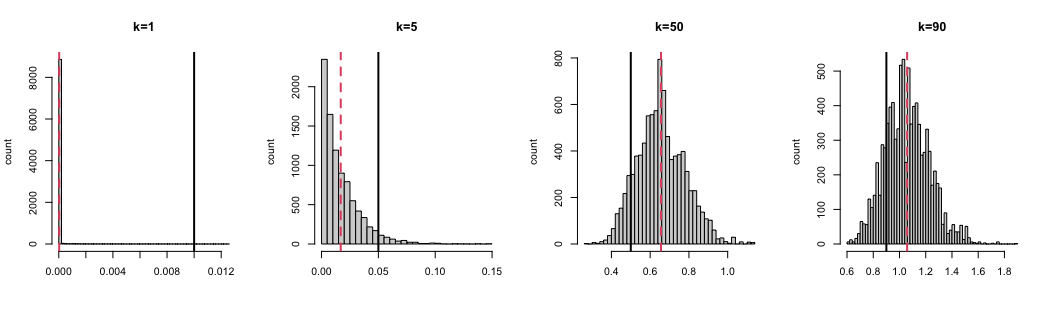
(a) ${\rm{PH}}(m=0,a=1,b=2,c=1)$

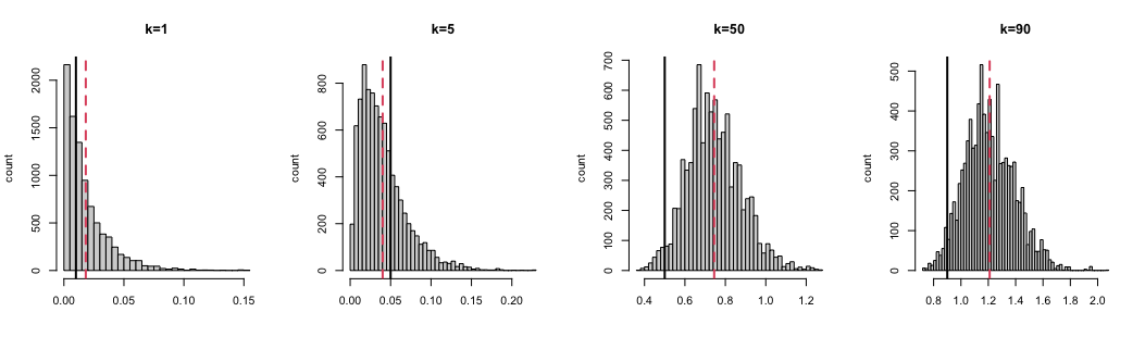
(b) ${\rm{PH}}(m=1,a=1,b=3,c=1)$

Figure 3: Posteriors of $\alpha_{k}$ from Setting 2. We include four $\alpha_{k}$ with $k=1,5,50,90$. The black solid vertical line marks the location of true $\alpha_{k}=k/K$ and the red dashed vertical line marks the posterior mean. In this specific example, $N_{1}=0$.

For Table 2, we observe that with more information, our horseshoe prior combined with heterogeneous modeling better captures the true values of ${\bm{\alpha}}$, irrespective of whether the true ${\bm{\alpha}}$ is homogeneous or heterogeneous. We include a plot of the posteriors under ${\rm{PH}}(m=0,a=1,b=2,c=1)$ prior and ${\rm{PH}}(m=1,a=1,b=3,c=1)$ from one repetition under Setting 2 in Figure 3, where the former prior induces bigger shrinkage than the latter. In this specific example, the first category $k=1$ has zero counts across all documents, i.e., $N_{1}=0$. Our prior effectively shrinks all posterior mass towards zero. For $k=5$, while the total number of counts is very small but non-zero, we observe a horseshoe-shaped posterior, indicating a strong shrinkage effect for small counts with ${\rm{PH}}(m=0,a=1,b=2,c=1)$, while the posterior mass shifts away from zero with the ${\rm{PH}}(m=1,a=1,b=3,c=1)$ prior. For $k=50$ and $k=90$, our posterior distributions exhibit a bell shape and cover the true values. The plot suggests that the heterogeneous shrinkage prior ${\rm{PH}}(m=0,a=1,b=2,c=1)$ helps the posterior properly adapt to both sparse and quasi-sparse counts.

4.3 Scenario 3: Multiple Documents with Structural Zeros

Here we consider cases where there are structural zeros in the dataset, i.e., a zero pattern that is shared by different documents and is different from events that have a positive probability but still observe a zero count. Note that our interpretation of structural zeros is different from the one in (Koslovsky, 2023). Instead of a two-component representation, we translate the event $\pi_{sk}=0$ to be $\alpha_{k}=0$ which is consistent with the conventional DM representation. For the “at-risk” zeros, which corresponds to $n_{sk}=0$ but $\pi_{sk}>0$, we believe that $\alpha_{k}>0$. To enforce the zero patterns, we initialize $\alpha_{k}=k/K$ and then randomly select a $q\%$ of the $\alpha_{k}$’s and let them be zero, so the category probabilities $\{\pi_{sk}\}$ sampled from these $\alpha_{k}$’s will always be zero. The results are reported in Table 3.

MTD	DM	Tuyl	ZIDM	PH 1-h	PH2-h	PH3-h	PH4-h	PH1-d	PH2-d	PH3-d	PH4-d
	Setting 1: $q=10\%$
ABS×100	0.503(0.009)	0.551(0.01)	16.203(0.974)	0.547(0.01)	0.547(0.01)	0.547(0.01)	0.547(0.01)	0.494(0.009)	0.493(0.009)	0.5(0.009)	0.499(0.009)
COV	0.846(0.004)	0.959(0.003)	0.959(0.003)	0.795(0.006)	0.795(0.006)	0.795(0.006)	0.795(0.006)	0.949(0.009)	0.95(0.009)	0.953(0.003)	0.954(0.003)
	Setting 2: $q=30\%$
ABS×100	0.457(0.014)	0.513(0.016)	17.514(1.084)	0.514(0.016)	0.514(0.016)	0.514(0.016)	0.514(0.016)	0.444(0.013)	0.443(0.013)	0.451(0.014)	0.45(0.014)
COV	0.656(0.004)	0.962(0.003)	0.966(0.003)	0.63(0.006)	0.63(0.006)	0.63(0.006)	0.63(0.006)	0.959(0.009)	0.96(0.009)	0.964(0.003)	0.965(0.003)
	Setting 3: $q=50\%$
ABS×100	0.41(0.013)	0.457(0.018)	20.432(1.543)	0.464(0.017)	0.464(0.018)	0.465(0.018)	0.464(0.018)	0.394(0.013)	0.393(0.013)	0.402(0.013)	0.401(0.013)
COV	0.468(0.003)	0.964(0.003)	0.974(0.003)	0.455(0.005)	0.455(0.005)	0.455(0.005)	0.455(0.005)	0.973(0.006)	0.973(0.006)	0.973(0.003)	0.974(0.003)

Table 3: Performance comparison of different posteriors from multiple documents with structural zeros. The bold fonts mark the lowest ABV in each setting.

In Table 3, we observe that as the percentage of structural zeros increases, the performance of ZIDM worsens, even though it provides valid coverage for the true probabilities, indicating wide credible intervals. Our choice of prior, ${\rm{PH}}(m=0,a=1,b=5,c=1)$, offers the best posterior mean estimates in all three settings, closely followed by the choice ${\rm{PH}}(m=0,a=1,b=2,c=1)$. Under the heterogeneous setting, all PH priors are able to provide valid coverage for true probabilities.

Combing the results in Table 2 and Table 3, we find that using the shrinkage prior ${\rm{PH}}(m=0,a=1,b=5,c=1)$ with heterogeneous ${\bm{\alpha}}$ yields optimal adaptability. While there is slight difference between priors ${\rm{PH}}(m=0,a=1,b=2,c=1)$ and ${\rm{PH}}(m=0,a=1,b=5,c=1)$, the performance overall is robust to the choice of $b$ and we recommend using the prior ${\rm{PH}}(m=0,a=1,b=2,c=1)$ for the strongest shrinkage effect. When there is insufficient information available, such as in the single document case in Table 1, we recommend using the prior ${\rm{PH}}(m=0,a=1,b=2,c=1)$ with homogeneous $\alpha$.

5 Empirical Analysis: Microbiome Compositional Data Analysis

One significant application of our method lies in understanding the sparsity patterns within microbiome datasets. The human microbiome comprises microorganisms inhabiting both the surface and internal parts of our bodies. Analyzing such data is challenging due to its compositional structure, over-dispersion, and zero-inflation. Consequently, the DM model and its variants have been widely utilized in this field. In addition, it is crucial to distinguish between structural zeros (indicating the absence of species) and sampling zeros (resulting from low sequencing depth or dropout).

To showcase the usefulness of our method, we employ the human gut microbiome dataset studied in Wu et al. (2011), containing 28 genera-level operational taxonomic unit counts obtained from 16S rRNA sequencing on 98 objects. There are over 30% zeros in the dataset.

The posterior mean estimates for the category probabilities under the ${\rm{PH}}(m=0,a=1,b=2,c=1)$ prior for heterogeneous ${\bm{\alpha}}$ is plotted in Figure 4. Four taxonomic units (LIS, EIS, RIS, PIS) are shown in abbreviation. We compare our results with alternative methods used in the simulation studies in Section 4 and find that the estimated probabilities are very similar. The average of absolute difference is below $1\times 10^{-4}$ between our method and ZIDM or Tuyl’s. For this dataset, we observe that Bacteroides predominates in most individuals, and its lower concentration often coincides with a higher concentration of Prevotella. The abundance levels of Lachnospiraceae Incertae Sedis (LIS), Subdoligranulum, Faecalibacterium, Alistipes, Parabacteroides, Peptostreptococcaceae Incertae Sedis (PIS) show noticeable variations across individuals, which could be potentially related to variations in individual covariates. We hope to explore these relationships in future extensions of this work.

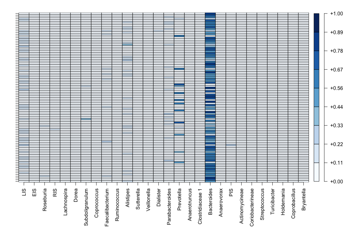
Figure 4: Posterior mean estimates for category probabilities from ${\rm{PH}}(m=0,a=1,b=2,c=1)$. Each row is a different individual and each column is a different taxonomic unit.

6 Discussion

In this work, we introduce a novel class of prior for the classical Dirichlet-Multinomial models. Our contributions are two-fold. First, instead of obtaining an empirical Bayes estimate or a maximum likelihood estimate (Minka, 2000) for ${\bm{\alpha}}$, we propose a conjugate prior for ${\bm{\alpha}}$ which enables full Bayesian inference for the DM models. The full posterior descriptions for ${\bm{\alpha}}$ ensure better uncertainty quantification. In the homogeneous $\alpha_{k}$ case, we show how a closed-form representation for the posterior density function and posterior moments can be obtained. The concentration parameter ${\bm{\alpha}}$ plays an important role in determining information sharing patterns in topic modeling such as Latent Dirichlet Allocation (LDA) models. However, it was common practice to choose homogeneous DM models due to the computational issues stemming from high-dimensional hyperparameters. Our PH priors provide an alternative to overcome these issues and thus allow for a more flexible formulation of LDA models.

Second, our priors provide a new approach for accommodating sparsity and quasi-sparsity in compositional count datasets. Under the configuration of $m=0$, our priors exhibit a horseshoe-shaped behavior, which guarantees super-efficient sparsity recovery. Our representation preserves the meaningful parameter ${\bm{\alpha}}$ while avoiding the complex two-groups mixture models. Furthermore, our method can be extended to regression settings, allowing the sparsity patterns to be explained by covariates. This is crucial for researchers in microbiome studies to understand the association between varying abundances and many diseases. By allowing individual-specific concentration parameter $\alpha_{sk}$, we can relate $\alpha_{sk}$ to individual covariates such that it can learn information from both category level and individual level. Under our setting, the structural zeros are translated into events where $\alpha_{sk}=0$, which naturally leads to $\pi_{sk}=0$, and the sampling zeros correspond to events where $n_{sk=0}$ but $\alpha_{sk}\neq 0$.

There are a number of promising avenues for future research. The Pochhammer prior distributions are also conjugate to a plethora of Bayesian models, especially the Poisson-Gamma mixture models, such as the Waring distribution (Irwin, 1968). Additionally, there are also many applications in nonparametric Bayes, for example, the Pitman-Yor process and the Ewens sampling formula (Crane, 2016). By learning the full posterior on the concentration parameter, ${\bm{\alpha}}$, we can capture complete uncertainty in the models while maintaining analytical tractability.

Appendix A Proofs

A.1 Proof of Theorem 2

Similar to the proof of Theorem 1, we evaluate the identity when $m\neq 0$

$$\alpha^{d}\prod_{s=1}^{m}(\alpha+s-1)=\sum_{i=1}^{b}\gamma^{(m,a,b,c,d)}_{i}\prod_{k=1,\;k\neq i}^{b}(c\alpha+a+k-1)$$

at the set of points $\alpha=-(a+i-1)/c$, yielding

$$\gamma^{(m,a,b,c,d)}_{i}=\frac{(1-a-i)^{d}\prod_{s=1}^{m}(1+(s-1)c-a-i)}{c^{m+d}\prod_{k=1,\;k\neq i}^{b}(k-i)}.$$

When $m=0$, similar we have the identity as

$$\alpha^{d}=\sum_{i=1}^{b}\gamma^{(m,a,b,c,d)}_{i}\prod_{k=1,\;k\neq i}^{b}(c\alpha+a+k-1),$$

the rest of the calculation follows through.

The normalizing constant $C_{(m,a,b,c,d)}$ can be computed in a similar fashion to $C$ as

$$C_{(m,a,b,c,d)}=\sum_{i=1}^{b}\int_{0}^{\infty}\frac{\gamma^{(m,a,b,c,d)}_{i}}{c\alpha+a+i-1}{\mathrm{d}}\alpha=\sum_{i=1}^{b}\frac{\Big{(}-\gamma^{(m,a,b,c,d)}_{i}\Big{)}}{c}\ln(a+i-1).$$

A.2 Double Roots

Consider a special case of the Pochhammer distribution with $a=0$

$$p(\alpha\mid m,a=0,b,c)=\frac{1}{C_{m,0,b,c}}\frac{[\alpha]^{m}}{[c\alpha]^{b}}.$$

From Theorem 1, we have

$$\gamma^{(m,0,b,c)}_{i}=\frac{\prod_{s=1}^{m}(1+(s-1)c-i)}{c^{m}\prod_{k=1,\;k\neq i}^{b}(k-i)},C_{(m,0,b,c)}=\sum_{i=2}^{b}\frac{\big{(}-\gamma^{(m,0,b,c)}_{i}\big{)}}{c}\ln(i-1)$$

From the first term, we see $\gamma^{(m,o,b,c)}_{1}=0$, so the sum in normalizing constant can be reduce to $\sum_{i=2}^{b}$. The mean and variance of the prior can be calculated using Theorem 2.

Theorem 4 (Posterior in Residues).

Under a Pochhammer prior $\alpha\sim{\rm{PH}}(m=n_{0},a=0,b,c=K)$, the posterior in (3) has closed-form as

$$p(\alpha\mid{\bm{n}})=C_{N}^{-1}\frac{\prod_{k=0}^{K}[\alpha]^{n_{k}}}{[K\alpha]^{N}[K\alpha]^{b}}=C_{N}^{-1}\left[\sum_{i=1}^{\max(N,b)}\frac{\gamma_{i}^{*}}{K\alpha+i-1}+\sum_{i=1}^{\min(N,b)}\frac{\beta_{i}^{*}}{(K\alpha+i-1)^{2}}\right]$$ (13)

where

$$\beta_{i}^{*} =\frac{\displaystyle\prod_{k=0}^{K}\prod_{s=1}^{n_{k}}\Big{(}1+K(s-1)-i\Big{)}}{\displaystyle K^{N+n_{0}}\prod_{s=1,\;s\neq i}^{\min(N,b)}(s-i)^{2}\prod_{t=1}^{\left|N-b\right|}(b+t-i)}\;\;\text{ for }1\leq i\leq\min(N,b)$$

$$\gamma_{i}^{*} =\left\{\begin{array}[]{l l}{\displaystyle K\beta_{i}^{*}\left(\sum_{k=0}^{K}\sum_{s=1}^{n_{j}=k}\frac{1}{1+K(s-1)-i}-\sum_{s=1,\;s\neq i}^{\min(N,b)}\frac{2}{s-i}-\sum_{t=1}^{\left|N-b\right|}\frac{1}{b+t-i}\right)}&\text{ for }1<i\leq\min(N,b)\\ \frac{\displaystyle\prod_{k=0}^{K}\prod_{s=1}^{n_{k}}\Big{(}1+K(s-1)-i\Big{)}}{\displaystyle K^{N+n_{0}}\prod_{s=1,\;s\neq i}^{\min(N,b)}(s-i)^{2}\prod_{t=1}^{\left|N-b\right|}(b+t-i)}&\text{ for }\min(N,b)<i\leq\max(N,b)\end{array}\right.$$

$$C_{N} =\sum_{i=2}^{\max(N,b)}\frac{-\gamma_{i}^{*}}{K}\ln(i-1)+\sum_{i=2}^{\min(N,b)}\frac{-\beta_{i}^{*}}{K(i-1)}.$$

Proof.

Without loss of generality, we assume $b\leq N$. Using the same residual argument, we can write the identity as

$$\begin{split}\prod_{k=0}^{K}[\alpha]^{n_{k}}=&\sum_{i=1}^{N}\gamma_{i}^{*}(K\alpha+i-1)\prod_{s=1,\;s\neq i}^{b}(K\alpha+s-1)^{2}\prod_{t=1}^{N-b}(K\alpha+b+t-1)\\ &+\sum_{i=1}^{b}\beta_{i}^{*}\prod_{s=1,\;s\neq i}^{b}(K\alpha+s-1)^{2}\prod_{t=1}^{N-b}(K\alpha+b+t-1).\end{split}$$

Again, by evaluating the above identity at $\alpha=-(i-1)/k$, we recover

$$\beta_{i}^{*} =\frac{\prod_{k=0}^{K}\prod_{s=1}^{n_{j}}\Big{(}1+K(s-1)-i\Big{)}}{K^{N+n_{0}}\prod_{s=1,\;s\neq i}^{b}(s-i)^{2}\prod_{t=1}^{N-b}(b+t-i)}\;\;\text{ for every }1\leq i\leq b$$

$$\gamma_{i}^{*} =\frac{\prod_{k=0}^{K}\prod_{s=1}^{n_{k}}\Big{(}1+K(s-1)-i\Big{)}}{K^{N+n_{0}}\prod_{s=1}^{b}(s-i)^{2}\prod_{t=1,\;t\neq i-b}^{N-b}(b+t-i)}\;\;\text{ for every }b<i\leq N$$

To calculate $\gamma_{i}^{*}$ for $1\leq i\leq b$, we use the method that

$$\gamma_{i}^{*}=\left.\left[\frac{{\mathrm{d}}}{{\mathrm{d}}\alpha}(K\alpha+i-1)^{2}\frac{\prod_{k=0}^{K}[\alpha]^{n_{k}}}{[K\alpha]^{N}[K\alpha]^{b}}\right]\right|_{\alpha=-(i-1)/K}$$

We use $N(\alpha)$ and $D(\alpha)$ to denote the denominator and numerator functions, respectively, as

$$N(\alpha) =\prod_{k=0}^{K}[\alpha]^{n_{k}}=\prod_{k=0}^{K}\prod_{s=1}^{n_{k}}(\alpha+s-1)$$

$$D(\alpha) =\prod_{s=1,\;s\neq i}^{b}(K\alpha+s-1)^{2}\prod_{t=1}^{N-b}(K\alpha+b+t-1),$$

then $\gamma_{i}^{*}$ can be written as

$$\gamma_{i}^{*}=\left.\left[\frac{N^{\prime}(\alpha)D(\alpha)-N(\alpha)D^{\prime}(\alpha)}{D(\alpha)^{2}}\right]\right|_{\alpha=-(i-1)/K}.$$ (14)

Next, we break down the calculation using the product rule

$$N^{\prime}(\alpha) =N(\alpha)\sum_{k=0}^{K}\sum_{s=1}^{n_{k}}\frac{1}{\alpha+s-1}$$

$$D^{\prime}(\alpha) =D(\alpha)\left(\sum_{s=1,\;s\neq i}^{b}\frac{2k}{K\alpha+s-1}+\sum_{t=1}^{N-b}\frac{K}{K\alpha+b+t-1}\right).$$

With the expression of $N^{\prime}(\alpha)$ and $D^{\prime}(\alpha)$ plugging into (14), we have

$$\gamma_{i}^{*} =\left.\left[\frac{N(\alpha)}{D(\alpha)}\left(\sum_{k=0}^{K}\sum_{s=1}^{n_{k}}\frac{1}{\alpha+s-1}-\sum_{s=1,\;s\neq i}^{b}\frac{2K}{K\alpha+s-1}-\sum_{t=1}^{N-b}\frac{K}{K\alpha+b+t-1}\right)\right]\right|_{\alpha=-(i-1)/K}.$$

$$=\frac{\prod_{k=0}^{K}\prod_{s=1}^{n_{k}}\big{(}1+K(s-1)-i\big{)}}{K^{N+n_{0}}\prod_{s=1,\;s\neq i}^{b}(s-i)^{2}\prod_{t=1}^{N-b}(b+t-i)}$$

$$\qquad\times\left(\sum_{k=0}^{K}\sum_{s=1}^{n_{k}}\frac{K}{1+K(s-1)-i}-\sum_{s=1,\;s\neq i}^{b}\frac{2K}{s-i}-\sum_{t=1}^{N-b}\frac{K}{b+t-i}\right)$$

$$=\frac{\prod_{k=0}^{K}\prod_{s=1}^{n_{j}}\big{(}1+K(s-1)-i\big{)}}{K^{N+n_{0}-1}\prod_{s=1,\;s\neq i}^{b}(s-i)^{2}\prod_{t=1}^{N-b}(b+t-i)}$$

$$\qquad\times\left(\sum_{k=0}^{K}\sum_{s=1}^{n_{k}}\frac{1}{1+K(s-1)-i}-\sum_{s=1,\;s\neq i}^{b}\frac{2}{s-i}-\sum_{t=1}^{N-b}\frac{1}{b+t-i}\right)\;\text{ for every }1\leq i\leq b.$$

Note that we have $\gamma_{1}^{*}=\beta_{1}^{*}=0$, the calculation of the normalizing constant $C_{N}$ is similar to previous argument as

$$C_{N} =\int_{0}^{\infty}\sum_{i=1}^{N}\frac{\gamma_{i}^{*}}{K\alpha+i-1}+\sum_{i=1}^{b}\frac{\beta_{i}^{*}}{(K\alpha+i-1)^{2}}\;{\mathrm{d}}\alpha$$

$$=\sum_{i=1}^{N}\frac{(-\gamma_{i}^{*})}{K}\ln(i-1)+\sum_{i=1}^{b}\frac{(-\beta_{i}^{*})}{K(i-1)}.$$

∎

A.3 Heterogeneous $\alpha_{k}$

Without further information, we assume the same Pochhammer prior ${\rm{PH}}(\alpha_{k}\mid m,a,b,c)$ for each $\alpha_{k},k=1,\ldots,K$. Then the posterior in (3) can be written as

$$p({\bm{\alpha}}\mid{\bm{n}})\propto\frac{1}{[A]^{N}}\prod_{k=1}^{K}\frac{[\alpha_{k}]^{n_{k}}[\alpha_{k}]^{m}}{[c\alpha_{k}+a]^{b}}$$

Denote $\displaystyle A_{-k}=\sum_{j=1,j\neq k}^{K}\alpha_{j}=A-\alpha_{k}$, Gibbs conditionals $\alpha_{k}$ given $\{\alpha_{j}\}_{j=1,j\neq k}^{K}$ can be written as

$$p(\alpha_{k}\mid{\bm{n}},A_{-k})\propto\frac{1}{[\alpha_{k}+A_{-k}]}\frac{[\alpha_{k}]^{n_{k}}[\alpha_{k}]^{m}}{[c\alpha_{k}+a]^{b}}$$

Using the same residual argument, the density function can be written explicitly as

$$p(\alpha_{k}\mid{\bm{n}},A_{-k})=C_{N,A_{-k}}^{-1}\left[\sum_{j=1}^{N}\frac{\gamma_{j}^{*}}{\alpha_{k}+A_{-k}+j-1}+\sum_{j=1}^{b}\frac{\beta_{j}^{*}}{c\alpha_{k}+a+j-1}\right]$$

where

$$\gamma_{j}^{*} =\frac{[-(A_{-k}+j-1)]^{n_{k}}[-(A_{-k}+j-1)]^{m}}{[-c(A_{-k}+j-1)+a]^{b}\prod_{t=s,s\neq j}^{N}(s-j)}$$

$$\beta_{j}^{*} =\frac{c^{N-n_{k}-m}\prod_{s=1}^{n_{k}}(1+(s-1)c-a-j)\prod_{s=1}^{m}(1+(s-1)c-a-j)}{\prod_{s=1,s\neq j}^{b}(t-j)\prod_{s=1}^{N}(1+(A_{-k}+s-1)c-a-j)}$$

$$C_{N,A_{-k}} =\sum_{j=1}^{N}{(-\gamma_{j}^{*})}\ln(A_{-k}+j-1)+\sum_{j=1}^{b}\frac{(-\beta_{j}^{*})}{c}\ln(\alpha_{k}+a+j-1)$$

Proof.

We evaluate the identity

$$[\alpha_{k}]^{n_{k}}[\alpha_{k}]^{m}=\sum_{j=1}^{N}\gamma_{i}^{*}\prod_{s=1,s\neq j}^{N}(\alpha_{k}+A_{-k}+s-1)[c\alpha_{k}+a]^{b}+\sum_{j=1}^{b}\beta_{i}^{*}\prod_{s=1,s\neq j}^{b}(c\alpha_{k}+a+s-1)[\alpha_{k}+A_{-k}]^{N}.$$

At the set of points $\alpha_{k}=-(A_{-k}+j-1)$, we have

$$\gamma_{j}^{*}=\frac{[-(A_{-k}+j-1)]^{n_{k}}[-(A_{-k}+j-1)]^{m}}{[-c(A_{-k}+j-1)+a]^{b}\prod_{t=s,s\neq j}^{N}(s-j)}.$$

At the set of points $\alpha_{k}=-(a+j-1)/c$, we have

$$\beta_{j}^{*}=\frac{c^{N-n_{k}-m}\prod_{s=1}^{n_{i}}(1+(s-1)c-a-j)\prod_{s=1}^{m}(1+(s-1)c-a-j)}{\prod_{s=1,s\neq j}^{b}(t-j)\prod_{s=1}^{N}(1+(A_{-k}+s-1)c-a-j)}$$

The normalizing constants is

$$C_{N,A_{-i}} =\sum_{j=1}^{N}\int_{0}^{\infty}\frac{\gamma_{j}^{*}}{\alpha_{k}+A_{-k}+j-1}{\mathrm{d}}\alpha_{k}+\sum_{j=1}^{b}\int_{0}^{\infty}\frac{\beta_{j}^{*}}{c\alpha_{k}+a+j-1}{\mathrm{d}}\alpha_{i}$$

$$=\sum_{j=1}^{N}{(-\gamma_{j}^{*})}\ln(A_{-k}+j-1)+\sum_{j=1}^{b}\frac{(-\beta_{j}^{*})}{c}\ln(a+j-1).$$

∎

References

- Armagan et al. (2011) Armagan, A., Clyde, M., and Dunson, D. (2011). Generalized beta mixtures of gaussians. Advances in neural information processing systems, 24.
- Armagan et al. (2013) Armagan, A., Dunson, D. B., and Lee, J. (2013). Generalized double pareto shrinkage. Statistica Sinica, 23(1):119.
- Barndorff-Nielsen et al. (1982) Barndorff-Nielsen, O., Kent, J., and Sørensen, M. (1982). Normal variance-mean mixtures and z distributions. International Statistical Review/Revue Internationale de Statistique, pages 145–159.
- Berger et al. (2015) Berger, J. O., Bernardo, J. M., and Sun, D. (2015). Overall objective priors. Bayesian Analysis, 10(1):189–221.
- Bhattacharya et al. (2015) Bhattacharya, A., Pati, D., Pillai, N. S., and Dunson, D. B. (2015). Dirichlet–laplace priors for optimal shrinkage. Journal of the American Statistical Association, 110(512):1479–1490.
- Blei et al. (2003) Blei, D. M., Ng, A. Y., and Jordan, M. I. (2003). Latent Dirichlet allocation. Journal of machine Learning research, 3(Jan):993–1022.
- Carvalho et al. (2010) Carvalho, C. M., Polson, N. G., and Scott, J. G. (2010). The horseshoe estimator for sparse signals. Biometrika, 97(2):465–480.
- Crane (2016) Crane, H. (2016). The ubiquitous Ewens sampling formula. Statistical Science, 31(1):1–19.
- Datta and Dunson (2016) Datta, J. and Dunson, D. B. (2016). Bayesian inference on quasi-sparse count data. Biometrika, 103(4):971–983.
- Deek and Li (2021) Deek, R. A. and Li, H. (2021). A zero-inflated latent dirichlet allocation model for microbiome studies. Frontiers in Genetics, 11:602594.
- George and Doss (2017) George, C. P. and Doss, H. (2017). Principled selection of hyperparameters in the Latent Dirichlet Allocation model. Journal of Machine Learning Research, 18(1):5937–5974.
- He et al. (2019) He, J., Polson, N. G., and Xu, J. (2019). Bayesian inference for gamma models. arXiv preprint arXiv:1905.12141.
- Irwin (1968) Irwin, J. O. (1968). The generalized waring distribution applied to accident theory. Journal of the Royal Statistical Society Series A: Statistics in Society, 131(2):205–225.
- Jeffreys (1939) Jeffreys, H. (1939). Theory of probability. Oxford University Press.
- Jeffreys (1946) Jeffreys, H. (1946). An invariant form for the prior probability in estimation problems. Proceedings of the Royal Society of London. Series A. Mathematical and Physical Sciences, 186(1007):453–461.
- Koslovsky (2023) Koslovsky, M. D. (2023). A Bayesian zero-inflated Dirichlet-multinomial regression model for multivariate compositional count data. Biometrics.
- Lambert (1992) Lambert, D. (1992). Zero-inflated poisson regression, with an application to defects in manufacturing. Technometrics, 34(1):1–14.
- Lidstone (1920) Lidstone, G. J. (1920). Note on the general case of the Bayes-Laplace formula for inductive or a posteriori probabilities. Transactions of the Faculty of Actuaries, 8(182-192):13.
- Liu et al. (2020) Liu, T., Zhao, H., and Wang, T. (2020). An empirical Bayes approach to normalization and differential abundance testing for microbiome data. BMC bioinformatics, 21:1–18.
- Miller (2019) Miller, J. W. (2019). Fast and accurate approximation of the full conditional for gamma shape parameters. Journal of Computational and Graphical Statistics, 28(2):476–480.
- Minka (2000) Minka, T. (2000). Estimating a Dirichlet distribution.
- Perks (1947) Perks, W. (1947). Some observations on inverse probability including a new indifference rule. Journal of the Institute of Actuaries, 73(2):285–334.
- Polson and Scott (2010) Polson, N. G. and Scott, J. G. (2010). Shrink globally, act locally: Sparse bayesian regularization and prediction. Bayesian statistics, 9(501-538):105.
- Polson et al. (2013) Polson, N. G., Scott, J. G., and Windle, J. (2013). Bayesian inference for logistic models using Pólya–Gamma latent variables. Journal of the American statistical Association, 108(504):1339–1349.
- Rossell (2009) Rossell, D. (2009). GaGa: A parsimonious and flexible model for differential expression analysis. The Annals of Applied Statistics, pages 1035–1051.
- Tang and Chen (2019) Tang, Z.-Z. and Chen, G. (2019). Zero-inflated generalized Dirichlet multinomial regression model for microbiome compositional data analysis. Biostatistics, 20(4):698–713.
- Tuyl (2018) Tuyl, F. (2018). A method to handle zero counts in the multinomial model. The American Statistician.
- Wallach (2006) Wallach, H. M. (2006). Topic modeling: beyond bag-of-words. In Proceedings of the 23rd international conference on Machine learning, pages 977–984.
- Wu et al. (2011) Wu, G. D., Chen, J., Hoffmann, C., Bittinger, K., Chen, Y.-Y., Keilbaugh, S. A., Bewtra, M., Knights, D., Walters, W. A., Knight, R., et al. (2011). Linking long-term dietary patterns with gut microbial enterotypes. Science, 334(6052):105–108.
- Xia and Doss (2020) Xia, W. and Doss, H. (2020). Scalable hyperparameter selection for latent dirichlet allocation. Journal of Computational and Graphical Statistics, 29(4):875–895.
- Yang et al. (2009) Yang, Z., Hardin, J. W., and Addy, C. L. (2009). Testing overdispersion in the zero-inflated Poisson model. Journal of statistical planning and inference, 139(9):3340–3353.
- Zeng et al. (2022) Zeng, Y., Pang, D., Zhao, H., and Wang, T. (2022). A zero-inflated logistic normal multinomial model for extracting microbial compositions. Journal of the American Statistical Association, pages 1–14.
- Zito et al. (2023) Zito, A., Rigon, T., and Dunson, D. B. (2023). Bayesian nonparametric modeling of latent partitions via Stirling-gamma priors. arXiv preprint arXiv:2306.02360.