Analyzing the Impact of Computation in Adaptive Dynamic Programming for Stochastic LQR Problem

Abstract

Adaptive dynamic programming (ADP) for stochastic linear quadratic regulation (LQR) demands the precise computation of stochastic integrals during policy iteration (PI). In a fully model-free problem setting, this computation can only be approximated by state samples collected at discrete time points using computational methods such as the canonical Euler-Maruyama method. Our research reveals a critical phenomenon: the sampling period can significantly impact control performance. This impact is due to the fact that computational errors introduced in each step of PI can significantly affect the algorithm’s convergence behavior, which in turn influences the resulting control policy. We draw a parallel between PI and Newton’s method applied to the Ricatti equation to elucidate how the computation impacts control. In this light, the computational error in each PI step manifests itself as an extra error term in each step of Newton’s method, with its upper bound proportional to the computational error. Furthermore, we demonstrate that the convergence rate for ADP in stochastic LQR problems using the Euler-Maruyama method is $O(h)$, with $h$ being the sampling period. A sensorimotor control task finally validates these theoretical findings.

1 Introduction

In recent years, discrete-time reinforcement learning (RL) has proven effective in various domains, such as games (silver2016mastering), large language models (OpenAI2023GPT4TR), etc. Despite these advances, most systems, whether in natural sciences like physics (einstein1905motion) and biology (szekely2014stochastic), in social sciences such as finance (wang2020continuous) and psychology (oravecz2011hierarchical), or in engineering fields including robotics (stager2016stochastic) and power systems (milano2013systematic), operate continuously in time and are inherently stochastic, governed by stochastic differential equations (SDEs). The complexity and continuous nature of these systems underscore the growing importance and necessity of using stochastic continuous-time RL approach, e.g., adaptive dynamic programming (ADP) algorithms (jiang2011approximate; jiang2014adaptive; bian2016adaptive; bian2018stochastic; bian2019continuous; wei2023continuous).

In practical applications, the model is often unknown, and accurately modeling and identifying SDEs is a complex task (allen2007modeling; gray2011stochastic; browning2020identifiability). For cases with unknown system dynamics, policy iteration (PI)-based methods have been proposed for stochastic linear quadratic regulator (LQR) problems that involve state and control-dependent noise (jiang2011approximate; jiang2014adaptive; bian2016adaptive; bian2018stochastic; bian2019continuous). A significant challenge with this method is that each PI step involves the computation of a stochastic integral, as detailed in Equation (6) in bian2016adaptive and also in eq.PIa. When the system is fully model-free, finding an exact analytical solution for this stochastic integral is not feasible due to the unknown analytical form of the integrand. For example, the analytical form of the integrand $x^{\top}\otimes x^{\top}$ in the integral $\int_{t}^{t+\delta_{t}}x^{\top}\otimes x^{\top}\rd s$ from eq.PIa is inaccessible since we cannot acquire the analytical form of the system state $x$.

An alternative approach is to approximate the integral with discrete-time state samples using numerical methods, such as the canonical Euler-Maruyama method (kloeden1992stochastic). Consider an autonomous driving car equipped with various sensors such as LIDAR, radar, and cameras, which collect data with a sampling period of $h$. By gathering these samples over a time span of $\delta_{t}=N_{s}h$, where $N_{s}$ is sample size, we can approximate the integral $\int_{t}^{t+\delta_{t}}x^{\top}\otimes x^{\top}\rd s$ in eq.PIa using the sensor data at points $x(t)$, $x(t+h)$, …, $x(t+(N_{s}-1)h))$, see $\int_{t}^{t+\delta_{t}}x^{\top}\otimes x^{\top}\rd s\approx\sum_{i=0}^{N_{s}-1}x^{\top}(t+ih)\otimes x^{\top}(t+ih)\cdot h$. In this scenario, the sampling period $h$ essentially serves as the time step in the Euler-Maruyama method to approximate the integral.

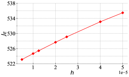
Figure 1: Expected cost $J_{E}$ for controllers, computed by the Euler-Maruyama method with varying sample period $h$ for a sensorimotor control task.

However, when applying the model-free ADP method to simulate a sensorimotor control task, as described in Section V of bian2016adaptive, we observe that the sample period $h$ in each interval can significantly impact the system’s performance. As illustrated in Figure 1, we find that as $h$ decreases, the expected cost $J_{E}=\mathbb{E}\left\{\int_{0}^{\infty}\left(x^{\top}Qx+u^{\top}Ru\right)\rd t\right\}$ decreases significantly. We analyze that the phenomenon “computation impacts control” can be attributed to the fact that a large sample period $h$ inevitably introduces computational errors when we approximate the stochastic integrals eq.PIa using samples collected at discrete time intervals. These computational errors can then lead to errors in each step of PI, accumulating throughout the entire PI process. Ultimately, this affects the convergence of ADP and consequently the control performance. To understand how computation influences control in ADP for stochastic LQR problems, we first examine the solution error in each step of PI due to computational errors and then quantify the cumulative impact throughout the PI process. Our contributions can be summarized as follows:

• We demonstrate that each step of PI necessitates the computation of stochastic integrals, which can only be approximated using samples collected at discrete time points. This approximation process inevitably introduces computational errors in each PI step. Taking advantage of the Euler-Maruyama method’s convergence properties and analyzing the matrix equation’s structure, we show that the solution error in each step of PI is proportional to the sampling period $h$, in a system with a fixed sampling period.

• We prove that the PI proposed in jiang2011approximate; jiang2014adaptive; bian2016adaptive can be interpreted as Newton’s method for solving the generalized Riccati equation. When impacted by computational errors, the PI process resembles Newton’s iteration with an additional error term. By leveraging the convergence properties of fixed-point iterations and assuming common Lipschitz conditions, we establish that the local convergence rate for ADP in stochastic LQR problems, in the presence of computational errors, is $O(h)$.

The remainder of this paper is organized as follows: In Section 2, we formulate the problem. Then, Section LABEL:sec.computational_error_analysis analyzes the computational error in the solution in each step of PI. Subsequently, Section LABEL:sec.convergence_analysis provides a detailed convergence analysis. Finally, we present the numerical results in Section LABEL:sec.results and conclude our paper in Section LABEL:sec.conclusion.

Notations: $\mathbb{R}^{m\times n}$ signifies the set of $m\times n$ real matrices. The symbol $\|\cdot\|$ specifically refers to the Euclidean norm when applied to vectors. The Frobenius norm for matrices is denoted by $\|\cdot\|_{F}$. We use $\mathrm{vec}(\cdot)$ to indicate the vectorization of a matrix, transforming it into a column vector. The Kronecker product operation is represented by $\otimes$. For matrix inequalities, $P\succ 0$ ($P\succeq 0$) means that matrix $P$ is positive (semi-)definite. The notation $|\cdot|$ is used for element-wise absolute value when applied to matrices or vectors.

2 Problem Formulation

Consider the linear system governed by the following SDE:

$$\rd x=(Ax+Bu)\rd t+B\rd w,$$ (1)

with

$$\rd w=\sum_{i=1}^{q_{1}}F_{i}x\rd w_{1i}+\sum_{i=1}^{q_{2}}G_{i}u\rd w_{2i}.$$ (2)

Here, $\bmatrix w_{1},&w_{2}^{\top}\in\mathbb{R}^{q_{1}+q_{2}}$ is the $\left\{\mathcal{F}_{t}\right\}$-adapted standard Brownian motion, where $\mathcal{F}_{t}$ is the $\sigma$-field generated by $\bmatrix w_{1},&w_{2}^{\top}$. Since accurately modeling and identifying the SDE as eq.SDE is a complex task (allen2007modeling; gray2011stochastic; browning2020identifiability), we consider a model-free problem setting, which means both $A\in\mathbb{R}^{n\times n}$, $B\in\mathbb{R}^{n\times m}$, $F_{i}\in\mathbb{R}^{m\times n}$ and $G_{i}\in\mathbb{R}^{m\times m}$ are unknown. Given $x(0)=x_{0}\in\mathbb{R}^{n}$, we consider the quadratic cost in LQR defined by

$$J(x_{0};u)=\mathbb{E}\left\{\int_{0}^{\infty}\left(x^{\top}Qx+u^{\top}Ru\right)\rd t|x_{0}\right\},$$

where $Q\succeq 0$ and $R\succ 0$. Suppose $\bmatrix A&BF_{1}BF_{2}...BF_{q_{1}}|\sqrt{Q}$ is observable (jiang2011approximate; jiang2014adaptive; bian2016adaptive; bian2018stochastic; bian2019continuous), the objective is to find the controller $u$ which minimizes $J(x_{0},u)$.

Definition 2.1 (Admissible matrix).

A matrix $K\in\mathbb{R}^{m\times n}$ is called admissible if the system described by eq.SDE and eq.SDE noise with control policy $u=-Kx$ is globally asymptotically stable (GAS) at the origin in the mean square sense (willems1976feedback) and $J(x_{0},u)<\infty,\forall x_{0}\in\mathbb{R}^{n}$.

[Admissible initial matrix] The system described by eq.SDE and eq.SDE noise is mean square stabilizable with a known admissible $K_{0}$ (jiang2011approximate; jiang2014adaptive; bian2016adaptive; bian2018stochastic; bian2019continuous).

It is shown in mclane1971optimal that $J(x_{0};u)$ is optimized under the optimal controller $u^{*}=-K^{*}x$, where $K^{*}=\left(\Sigma_{P^{*}}+R\right)^{-1}B^{\top}P^{*}$ and $P^{*}\in\mathbb{R}^{n\times n}$ is the unique symmetric positive definite solution to the following generalized algebraic Riccati equation

$$\mathcal{T}_{P}=0,$$ (3a)

with

$$\mathcal{T}_{P} :=A^{\top}P+PA-PB(\Sigma_{P}+R)^{-1}B^{\top}P+\Pi_{P}+Q,$$ (3b)

$$\Pi_{P} :=\Sigma_{i=1}^{q_{1}}F_{i}^{\top}B^{\top}PBF_{i},\;\quad\Sigma_{P}:=\Sigma_{i=1}^{q_{2}}G_{i}^{\top}B^{\top}PBG_{i}.$$

In situations where the system models are fully unknown, the data-driven PI approach can be utilized to solve the Riccati equation (jiang2011approximate; jiang2014adaptive; bian2016adaptive; bian2018stochastic; bian2019continuous). In the $k$-th step of PI, the control policy $u_{k}=-K_{k}x+e_{k}$, where $e_{k}$ represents the exploration noise, generates the data. The $k$-th step of PI can specifically be expressed as: