Does bilevel optimization result in more competitive racing behavior?

Abstract

Two-vehicle racing is natural example of a competitive dynamic game. As with most dynamic games, there are many ways in which the underlying information pattern can be structured, resulting in different equilibrium concepts. For racing in particular, the information pattern assumed plays a large impact in the type of behaviors that can emerge from the two interacting players. For example, blocking behavior is something that cannot emerge from static Nash play, but could presumably emerge from leader-follower play. In this work, we develop a novel model for competitive two-player vehicle racing, complete with simplified aerodynamic drag and drafting effects, as well as position-dependent collision-avoidance responsibility. We use this model to explore the impact that different information patterns have on the resulting competitiveness of the players. A solution approach for solving bilevel optimization problems is developed, which allows us to run a large-scale empirical study comparing how bilevel strategy generation (both as leader and as follower) compares with Nash equilibrium strategy generation as well as a single-player, constant velocity prediction baseline. Each of these choices are evaluated against different combinations of opponent strategy selection method. The somewhat surprising results of this study are discussed throughout.

I Introduction

Game-theoretic motion planning has emerged recently as a promising way to handle interactions among multiple agents in a principled manner, with many works exploring various related ideas. However, there still remains some open questions about the best way to formulate the trajectory games played between agents. The simplest and most common approach is to cast the interaction as a Generalized Nash Equilibrium Problem [17, 2, 12, 10, 18], but there are known deficiencies with such a formulation. Neither player in the game can reason about how its actions will illicit actions in response from its peers.

Some researchers have proposed posing games as repeated games and solving for Generalized Feedback Nash Equilibria [16, 9, 15] to try and capture some intelligent reasoning lacking in static Nash equilibria. However, feedback equilibria are extremely challenging to solve for, and it is not clear how much benefit comes from using the more elaborate information pattern.

Between repeated games and static games on the information pattern spectrum are Stackelberg games, in which one player is designated the leader, and the other players are designated as followers. Leading players can reason about how the actions of the followers will change as a function of their own actions, but the reverse is not true. Some existing works have studied bilevel optimization in the context of two-player games, leveraging the leader-follower dynamic to produce competitive behavior such as blocking [18]. However, that work and others have generally struggled to compute true Stackelberg equilibria in the full, constrained trajectory space, likely due to the inherent complexity of solving bilevel optimization problems. Even if such problems could be solved, it is not clear which player should be deemed the leader and which the follower. These distinctions are baseless in real-world situations where the players do not coordinate their roles.

We believe that there is a benefit to be gained from advanced information patterns, but that there exists a gap in the literature exploring to what degree are those benefits felt, and in which contexts. This purpose of this study is to make progress towards closing that gap, by performing a large scale empirical analysis on the benefits gained from computing trajectories via bilevel reasoning vs. static reasoning (as well as vs. a single-player optimization baseline). We have chosen to focus only on these simple strategy selection options because even for these relatively basic information patterns, the cost and benefits of choosing one or the other is not well understood. Furthermore, we believe that Stackelberg equilibria are the simplest (in terms of computation) formulation of game that is still capable of reasoning about action and reaction. Our belief is that the results of the study we perform can serve as a foundation that future studies comparing more information patterns can be based upon.

Specifically, the contributions we make in this paper are:

1. We present a large scale empirical study analyzing the performance and robustness of 16 different types of two-player racing competitions corresponding to different combination of information patterns assumed by each player: (1) Single-player optimization, (2) generalized Nash equilibrium, (3) Stackelberg equilibrium as a leader, or (4) Stackelberg equilibrium as a follower.

2. We implement a solver for nonlinear, large-scale bilevel constrained optimization problems, to enable the analysis above.

3. We derive a novel two-player racing formulation which involves position-dependent collision-avoidance responsibility as well as aerodynamic drag and drafting effects. This formulation captures the interesting competitive aspects of racing, allowing the various information patterns to be distinguished in intuitive ways.

This paper is organized as follows: In Section II, we provide the necessary game theory background, and define different types of competition that correspond to different combination of information structures. In Section III, we discuss solving bilevel problems and some limitations. In Section IV, we describe the racing dynamics with positional constraint bounds to encourage dynamic and competitive behavior. In Section V, we detail our large scale empirical study to analyze 16 different types of competition, and discuss the results.

II Game Theory Background

This work will be primarily concerned with two formulations of a two-player mathematical game. Consider two decision-makers, denoted by player $1$ and player $2$. Each player $i$ is associated with a set of decision variables $x_{i}\in\mathbb{R}^{n_{i}}$, which we denote as the private decision variables for that player. The joint set of decision variables are simply denoted by $x\in\mathbb{R}^{n}:=[x_{1}^{\intercal},x_{2}^{\intercal}]^{\intercal}$, where $n=n_{1}+n_{2}$. We will use the shorthand notation $(x_{i},x_{-i})\equiv x$ for both players, and generally use the index $-i$ to refer to player $2$ when $i=1$ and vice-versa.

The decision that each player attempts to make is characterized by a continuous, twice differentiable cost function $f_{i}:\mathbb{R}^{n}\to\mathbb{R}$, and a feasible region defined by $C_{i}:=\{x\in\mathbb{R}^{n}:g_{i}(x)\geq 0\}$, where $g_{i}:\mathbb{R}^{n}\to\mathbb{R}^{m_{i}}$ is a vector-valued constraint function, and is also continuous and twice-differentiable.

For either player $i$, the standard solution graph for their decision problem is defined as

$$S_{i}:=\left\{\begin{aligned} x^{*}\in\mathbb{R}^{n}\ :\ x^{*}_{i}\in&\operatorname*{\arg\!\min}_{x_{i}}&&f_{i}\left(x_{i},x^{*}_{-i}\right)\\ &\ \ \ \ \text{s.t.}&&\left(x_{i},x^{*}_{-i}\right)\in C_{i}\end{aligned}\right\}$$ (1)

In this work, the minimization appearing in Eq. 1 and all other problems will be assumed to be in the local sense unless otherwise specified. The solution graph $S_{i}$ is then the set of all points $x_{i}^{*}$ which are local optimizers for the decision problem parameterized by $x_{-i}^{*}$.

A point $x^{*}\in\mathbb{R}^{n}$ is called a local Generalized Nash Equilibrium Point if

$$x^{*}\in S_{1}\cap S_{2}.$$ (2)

A Generalized Nash Equilibrium Problem is to compute a point $x^{*}$ such that it satisfies Eq. 2 [19, 5, 1, 7]. For brevity, we will often drop the label “generalized” and refer to these equilibria and problems only by Nash.

For either player $i$, we define the bilevel solution graph as

$$B_{i}:=\left\{\begin{aligned} x^{*}\in\mathbb{R}^{n}\ :\ x^{*}\in&\operatorname*{\arg\!\min}_{x}&&f_{i}\left(x\right)\\ &\ \ \ \ \text{s.t.}&&x\in C_{i}\\ &&&x\in S_{-i}\end{aligned}\right\}$$ (3)

The bilevel solution graph for player $i$ is the set of all points which are local optimizers for the bilevel problem in which player $i$ is the leader and player $-i$ is the follower. The points

$$x^{*}\in B_{i}$$ (4)

are referred to as bilevel equilibrium points, and a bilevel equilibrium problem is the problem of finding a bilevel equilibrium.

In duopoly theory from the economics literature, Generalized Nash Equilibrium Problems are analogous with finding equilibrium points for Cournot competition [3], and bilevel optimization problems are analogous with finding equilibrium points for a Stackelberg competition [20]. These comparisons are relevant to the question we investigate in this work because it has been shown that Stackelberg duopolies generally result in an increase in total welfare compared to Cournot duopolies [11, 4]. We investigate whether a similar result is true for Bilevel or Nash competitions in the physical racing domain.

III Computing Solutions to Equilibrium Problems

In this section we present methodologies for computing Nash and bilevel equilibrium points.

III-A Nash Equilibrium Points

We assume that a suitable constraint qualification is satisfied for the problems Eq. 1. Then invoking the KKT theorem [13, 14], first-order necessary conditions which must be satisfied for every point $x^{*}\in S_{i}$ can be expressed as the following:

$$x^{*}\in S_{i} \implies\exists\lambda_{i}\in\mathbb{R}^{m_{i}}:(x^{*},\lambda_{i})\in\overline{S_{i}},$$ (5)

where

$$\overline{S_{i}}:=\left\{\begin{aligned} (x^{*},\lambda_{i}):&\ \nabla_{x_{i}}f_{i}(x^{*})-(\nabla_{x_{i}}g_{i}(x^{*}))^{\intercal}\lambda_{i}=0\\ &\ 0\leq g_{i}(x^{*})\perp\lambda_{i}\geq 0.\end{aligned}\right\}.$$ (6)

Here, $0\leq a\perp b\geq 0$ for $a,b\in\mathbb{R}^{m}$ means $a_{i}\geq 0$, $b_{i}\geq 0$, and $a_{i}b_{i}=0\ \forall i\in\{1,...,m\}$.

Combining Eqs. 5, 6 and 2, we have the following:

$$x^{*}\in S_{1}\cap S_{2}\implies \exists\lambda\in\mathbb{R}^{m_{1}+m_{2}}:$$ (7)

$$F(z)\perp l\leq z\leq u,$$

where

$$z :=\begin{bmatrix}x^{*}\\ \lambda\end{bmatrix}, F(z) :=\begin{bmatrix}\nabla_{x_{1}}f_{1}(x^{*})-(\nabla_{x_{1}}g_{1}(x^{*}))^{\intercal}\lambda_{1}\\ \nabla_{x_{2}}f_{2}(x^{*})-(\nabla_{x_{2}}g_{2}(x^{*}))^{\intercal}\lambda_{2}\\ g_{1}(x^{*})\\ g_{2}(x^{*})\end{bmatrix}$$ (8)

$$l :=\begin{bmatrix}0\\ 0\end{bmatrix} u :=\begin{bmatrix}0\\ \infty\end{bmatrix}.$$

The first and second elements appearing in $l$ and $u$ are vectors of dimension $n$ and $m=m_{1}+m_{2}$, respectively, and Eq. 7 means,

$$\forall i\in\{1,\cdots,n+m\},\begin{cases}F_{i}(z)=0,l_{i}<z_{i}<u_{i},&\ \mathrm{or}\\ F_{i}(z)>0,l_{i}=z_{i},&\ \mathrm{or}\\ F_{i}(z)<0,z_{i}=u_{i}.\end{cases}$$ (9)

It is seen then that the conditions Eq. 7 form a mixed complementarity problem [8]. In this work we use the PATH Solver [6] to find solutions $z^{*}$ to Eq. 7. Any such point is not necessarily a Nash equilibrium point Eq. 2, since in general the necessary conditions Eq. 5 are necessary but sufficient for optimality. Nevertheless, points satisfying Eq. 7 are often used as a proxy for Nash equilibrium points, and we will do the same for the purposes of this work.

III-B Bilevel Equilibrium Points

In contrast to the necessary-condition approach to Nash equilibrium problems, we will define sufficient conditions for bilevel equilibrium points.

First, note that $S_{i}\subset\{x:\exists\lambda,(x,\lambda)\in\overline{S_{i}}\}$. Therefore the sets $B_{i}$ can be approximated by replacing the constraint involving $S_{-i}$ with the less restrictive constraint:

$$\overline{B_{i}}:=\left\{\begin{aligned} x^{*}:\ \exists\lambda^{*},(x^{*},\lambda^{*})\in&\operatorname*{\arg\!\min}_{x,\lambda}&&f_{i}\left(x\right)\\ &\ \ \ \ \text{s.t.}&&x\in C_{i}\\ &&&\left(x,\lambda\right)\in\overline{S_{-i}}\end{aligned}\right\}.$$ (10)

However, it can be seen that if $x^{*}\in S_{-i}\cap\overline{B_{i}}$, then it must also be that $x^{*}\in B_{i}$. Therefore we pursue characterizing the points within $\overline{B_{i}}$.

$$x^{*}\in S_{-i}\cap\overline{B_{i}}\implies x^{*}\in B_{i}$$ (11)

Note that the sets $\overline{S_{i}}$ can be expressed as a union of simpler sets which involve only inequality constraints similar to the sets $C_{i}$. Specifically,

$$\overline{S_{i}}:=\bigcup_{k\in K}\overline{S_{i,k}},$$ (12)

where the sets comprising the union have the form

$$\overline{S_{i,k}}:=\left\{\begin{aligned} &F_{j}(z)=0,l_{j}\leq z_{j}\leq u_{j},&j\in J_{1}\\ &F_{j}(z)\geq 0,l_{j}=z_{j},&j\in J_{2}\\ &F_{j}(z)\leq 0,z_{j}=u_{j},&j\in J_{3}\end{aligned}\right\},$$ (13)

for some appropriately sized index sets $J_{1}$,$J_{2}$, $J_{3}$. Interpreting the set $\overline{S_{i}}$ via this union comes from enumerating the possible ways the conditions Eq. 9 can be satisfied. Using this union definition, the minimization appearing in Eq. 10 can be seen to be generally of a form

$$\min_{x} f(x)$$ (14)

$$\mathrm{s.t.} x\in\bigcup_{k\in K}D_{k}.$$

The following lemma allows us to reason about local optima of Eq. 14.

Lemma 1.

Let the sets $D_{k}$ appearing in Eq. 14 be closed sets. Then a point $x^{*}$ is a local optimum of Eq. 14 if and only if $x^{*}$ is a local optimum of all problems

$$\min_{x\in D_{k}}f(x),$$ (15)

for all $k$ such that $x^{*}\in D_{k}$.

The intuition behind this lemma is simple: If there are no local regions to descend within the unioned feasible set, then it follows no individual set in the union would offer a descent direction either. Conversely, if none of the local regions offer a descent direction, the union cannot offer a descent direction locally to $x^{*}$ either.

Proof of Lemma 1.

Let $D:=\bigcup_{k\in K}D_{k}$. Furthermore, let

$$\gamma_{D}(x):=\{k\in K:x\in D_{k}\}.$$ (16)

By definition, a point $x^{*}$ is a local optimum for (14) iff $x^{*}\in D$ and there exists some $\epsilon>0$ such that

$$f(x^{*})\leq f(x)\ \forall x\in D:\|x-x^{*}\|<\epsilon.$$ (17)

Since the sets $D_{k}$ are all closed, their complements are open, and therefore for sufficiently small choice of $\epsilon$,

$$x\notin D_{k}\ \forall k\notin\gamma_{D}(x^{*}).$$ (18)

Using such a choice of $\epsilon$, the definition in (17) can be rewritten as

$$f(x^{*})\leq f(x)\ \forall x\in D_{k}:\|x-x^{*}\|<\epsilon,k\in\gamma_{D}(x^{*}).$$ (19)

Since $x^{*}\in D_{k}\ \forall k\in\gamma_{D}(x^{*})$, this is equivalent to $x^{*}$ being a local optimum for each of the problems (15). ∎

This result inspires yet another set related to the bilevel solution graph, now only using a single component $\overline{S_{-i,k}}$ of the larger set of stationary points.

$$\overline{B_{i,k}}=\left\{\begin{aligned} x^{*}:\exists\lambda^{*},(x^{*},\lambda^{*})\in&\operatorname*{\arg\!\min}_{x,\lambda}&&f_{i}\left(x\right)\\ &\ \ \ \ \text{s.t.}&&x\in C_{i}\\ &&&\left(x,\lambda\right)\in\overline{S_{-i,k}}\end{aligned}\right\}$$ (20)

Leveraging Lemma 1 and the sets Eq. 20, an algorithm to check if a candidate point $x^{*}$ is a bilevel equilibrium or not can be derived. The basic procedure is as follows. First, identify a pair $(x,\lambda)\in S_{-i}\subset\overline{S_{-i}}$, by solving the follower’s optimization problem. Then enumerate all local regions Eq. 13, i.e. those such that $(x,\lambda)\in\overline{S_{-i,k}}$. For each of these regions and associated indices $k$, check to see if $(x,\lambda)$ is an element of $\overline{B_{i,k}}$. If the point belongs to all sets, then it must be an element of $\overline{B_{i}}$. This procedure is developed into an algorithm for computing bilevel equilibrium points in Algorithm 1.

Algorithm 1 Computing Bilevel Equilibria (for Player $1$)

Initial solution guess $x^{*}$

while not solved do

     $(x^{*}_{2},\lambda)\leftarrow$ solution to player 2’s optimization given $x_{1}^{*}$

     $K\leftarrow$ index set so that $(x^{*},\lambda)\in\overline{S_{2,k}}\ \forall k\in K$

     all agree $\leftarrow$ true

     for $k\in K$ do

         if $(x^{*},\lambda)\notin\overline{B_{i,k}}$ then

              all agree $\leftarrow$ false

              $(x^{*},\lambda)\leftarrow$ solution problem in $\overline{B_{i,k}}$

         end if

     end for

     if all agree then

         Return $x^{*}$

     end if

end while

IV Two-player Racing Game

Physical racing is a competition of speed, which can be held in many physical domains, provided that a human-controlled or autonomous vehicle can move in it. The vehicles must operate at their dynamic limits in racing, and they must plan and execute motions in close proximity to the other vehicles. In this section, we describe a two-player racing game, where the players are generic vehicles moving in the plane.

Our racing game consists of two players in simple motion in the horizontal plane constrained in a longitudinal track with minimum and maximum road limits in the lateral direction. The players control their longitudinal and lateral accelerations, and the players are encouraged to make forward progress. The players must avoid colliding with each other and remain within the road limits. The acceleration and collision constraints are the key driving factors of the competitive interactions, because they depend directly on the opponent player’s actions and current state, which the ego player cannot manipulate directly. We consider racing of two players on a straight road with no lanes.

We assume that there is no cooperation between the players. The racing game is played at every simulation step, and every simulation step each player chooses their control inputs for the next $n_{T}$ number computation horizon time steps. It falls under the category of repeated finite games. In the following sections we describe the vehicle dynamics model, then the objective functions and constraints of the players, followed by a detailed description of the positional constraints.

IV-A Vehicle Dynamics Model

The vehicle dynamics is simple motion described as a second-order differential equation, where the players manipulate their own lateral and longitudinal accelerations. We include a linear forcing term as a function of the player velocity as a crude model of velocity-dependent drag, and use Euler integration to discretize the differential dynamics. Let $p_{i}\in\mathbb{R}^{2}$ refer to the $i$^th player’s position in the plane, and let $\dot{p}_{i}=\mathrm{d}p_{i}/\mathrm{d}t$ be the $i$^th player’s velocity. Let $y_{i}$ be to the vehicle state and $u_{i}$ be the input for the $i$^th player,

$$y_{i} =\begin{bmatrix}p_{i}\\ \dot{p}_{i}\end{bmatrix}\in\mathbb{R}^{4},$$

$$u_{i} =\ddot{p}_{i}\in\mathbb{R}^{2}.$$

We discretize the differential motion problem using Euler integration and formulate the dynamics as a nonlinear constraint. We refer to the joint set of dynamic states using $y\in\mathbb{R}^{8}:=[y_{1}^{\intercal},y_{2}^{\intercal}]^{\intercal}$. Now we can write the difference equations that relate the dynamics and to the control inputs at the $k$^th time step,

$$y[k+1]=\begin{bmatrix}p_{1}^{k}+\Delta t\;\dot{p}_{1}[k]+\frac{1}{2}\Delta t^{2}\;(u_{1}[k]-c_{d}\;\dot{p}_{1}[k])\\ \dot{p}_{1}[k]+\Delta_{t}\;(u_{1}[k]-c_{d}\;\dot{p}_{1}[k])\\ p_{2}^{k}+\Delta t\;\dot{p}_{2}[k]+\frac{1}{2}\Delta t^{2}\;(u_{2}[k]-c_{d}\;\dot{p}_{2}[k])\\ \dot{p}_{2}[k]+\Delta_{t}\;(u_{2}[k]-c_{d}\;\dot{p}_{2}[k]).\end{bmatrix}$$

The private decision variables of each player at $k$^th simulation step is the player’s state and control variables for the next $n_{T}$ time steps in the future,

$$x_{1}[k] =\begin{bmatrix}\begin{bmatrix}y_{1}[k+1]^{\intercal},\cdots,y_{1}[k+n_{T}]^{\intercal}\end{bmatrix}^{\intercal}\\ \begin{bmatrix}u_{1}[k+1]^{\intercal},\cdots,u_{1}[k+n_{T}]^{\intercal}\end{bmatrix}^{\intercal}\end{bmatrix}\in\mathbb{R}^{6n_{T}},$$

$$x_{2}[k] =\begin{bmatrix}\begin{bmatrix}y_{2}[k+1]^{\intercal},\cdots,y_{2}[k+n_{T}]^{\intercal}\end{bmatrix}^{\intercal}\\ \begin{bmatrix}u_{2}[k+1]^{\intercal},\cdots,u_{2}[k+n_{T}]^{\intercal}\end{bmatrix}^{\intercal}\end{bmatrix}\in\mathbb{R}^{6n_{T}}.$$

The total number of the joint set of decision variables is $n=12n_{T}$. We omit the $k$^th time step in the square brackets where there is no room for confusion.

IV-B Objective Functions and Constraints

The objective function of each player involves three components to be summed over the next $n_{T}$ time steps as a running cost: (i) a quadratic penalty for being away from center of the road, (ii) another quadratic penalty for the control effort, (iii) and a linear penalty for the relative value of the opposing player’s longitudinal velocity. The linear relative velocity penalty term is positive when the opposing player velocity is greater than the ego player’s velocity, and vice versa. Because the velocity penalty term depends directly on the opponent’s actions and current state, and it is the most competitive component of the cost. The first quadratic penalty encourages each player to stay in the middle of the road. The second quadratic penalty discourages wasting control effort. Each player’s preference is modeled using a twice differentiable continuous cost function,

$$f_{1}(x) =\sum_{t=k+1}^{k+n_{T}}\alpha_{1}\,{y_{1}^{\text{lat}}}^{2}+\alpha_{2}\,u_{1}^{\intercal}u_{1}+\beta\left(\dot{y}_{2}^{\text{long}}-\dot{y}_{1}^{\text{long}}\right),$$

$$f_{2}(x) =\sum_{t=k+1}^{k+n_{T}}\alpha_{1}\,{y_{2}^{\text{lat}}}^{2}+\alpha_{2}\,u_{2}^{\intercal}u_{2}+\beta\left(\dot{y}_{1}^{\text{long}}-\dot{y}_{2}^{\text{long}}\right),$$

where superscripts “lat” and “long” refer to lateral and longitudinal position or velocity, respectively.

Each player has $\mathbb{R}^{4n_{T}}$ equality constraints for their dynamics, $\mathbb{R}^{n_{T}}$ inequality constraints for spatial collision $g_{i}^{\text{col}}(x_{1},x_{2})$, $\mathbb{R}^{2n_{T}}$ inequality constraints for lateral position to stay within the road limits, $\mathbb{R}^{n_{T}}$ inequality constraints for minimum longitudinal velocity to prevent going the wrong way, and $\mathbb{R}^{4n_{T}}$ inequalities for lateral and longitudinal acceleration limits $g_{i}^{\text{accel}}(x_{1},x_{2})\geq\mathbf{0}$. The responsibility of avoiding spatial collections is determined by the relative longitudinal position of the players. Additionally, the longitudinal acceleration constraint is a function of the opponent’s position, and it is intended to encourage competitive interaction in close proximity.

IV-C Spatial Collision Avoidance and Responsibility

The spatial collision avoidance constraint enforces minimum radial distance between the positions of the players. While collision avoidance is represented as a constraint that depends on the position of both players, and it is in the interest of both players to avoid a collision, the responsibility of collision avoidance is shared only sometimes. The responsibility of spatial collision avoidance is determined by the relative longitudinal position of the players. We assume that the responsibility of collision avoidance falls to the player that is behind in terms of longitudinal position. The responsibility is modeled using a custom responsibility function $h_{i}(x_{1},x_{2})$ for the $i$^th player that uses two scaled sigmoid functions to allow for a transition region for when the players are approximately side by side. During the transition period, the responsibility of collision falls onto the both players as a shared constraint, as shown in Fig. 2. We use positional constraints to set the lower bound of the collision constraint. Let the minimum desired radial distance between the players to be $r$,

$$g_{1,k}^{\text{col}}(x) =\begin{matrix}\lVert p_{1}-p_{2}\rVert^{2}-r^{2}-\ell_{1}(y_{2}^{\text{long}}-y_{1}^{\text{long}})\end{matrix}\geq 0,$$

$$g_{2,k}^{\text{col}}(x) =\begin{matrix}\lVert p_{1}-p_{2}\rVert^{2}-r^{2}-\ell_{2}(y_{2}^{\text{long}}-y_{1}^{\text{long}})\end{matrix}\geq 0,$$

$$\ell_{1}(h) =\frac{1}{1+e^{ah+b}}-\frac{1}{1+e^{b}},$$

$$\ell_{2}(h) =\frac{1}{1+e^{-ah+b}}-\frac{1}{1+e^{b}},$$

where $\lVert\cdot\rVert$ refers to the Euclidean norm, and $a$ and $b$ are parameters to adjust the slope of the sigmoid function near zero.

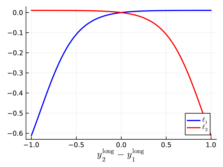
Figure 1: $\ell_{1}$ and $\ell_{2}$ with respect to relative longitudinal position of the players, note that the maximum of $\ell_{1}$ and $\ell_{2}$ is always non-negative, and is bounded to a small positive value, therefore $\lVert p_{1}-p_{2}\rVert^{2}\geq r^{2}$ for all values of relative longitudinal position.

The collision constraint is enforced for every time step $k\in\{t+1,\cdots,t+n_{T}\}$, such that $g_{i}=\begin{bmatrix}g_{i,t}^{\intercal},\cdots,g_{i,t+n_{T}}^{\intercal}\end{bmatrix}^{\intercal}$. When $y_{2}^{\text{long}}-y_{1}^{\text{long}}\geq 0$ (P2 is ahead), then $\ell_{1}(h)\geq 0$, $\ell_{2}(h)\leq 0$ and so, $g_{2}^{\text{col}}$ is relieved. Conversely, when $y_{2}^{\text{long}}-y_{1}^{\text{long}}\leq 0$ (P1 is ahead), then $\ell_{1}(h)\leq 0$, $\ell_{2}(h)\geq 0$ and so, $g_{1}^{\text{col}}$ is relieved. Additionally, we make the desired radial distance to include a small buffer than the minimum collision distance that we use to terminate simulations for collisions at every simulation time step.

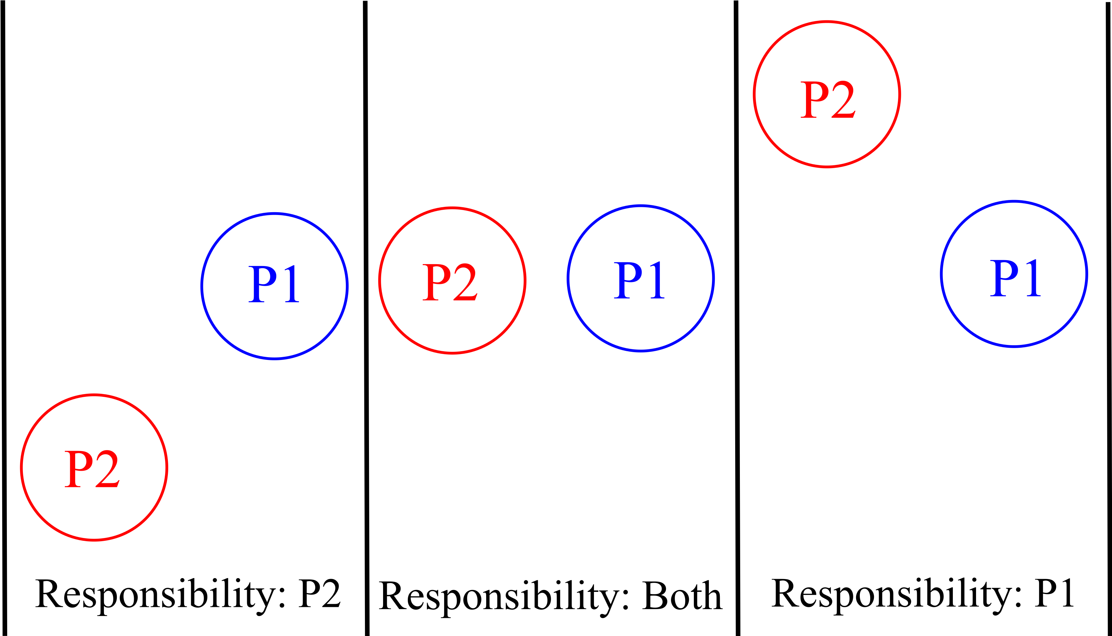
Figure 2: Responsibility of spatial collision avoidance falls on the player who is trailing, unless the players are side by side.

IV-D Drafting for Acceleration Limits

In order to encourage dynamic competitive behavior in our racing model, we use positional constraint bounds on the acceleration limits for both players. Firstly, we consider a linear drag as a function of velocity that apply to both players forcing them to exert control effort to maintain their velocity. Then, we define a smooth rectangular region behind each player that boosts the opponent’s acceleration limits which was loosely inspired by the aerodynamics of real-life racing.

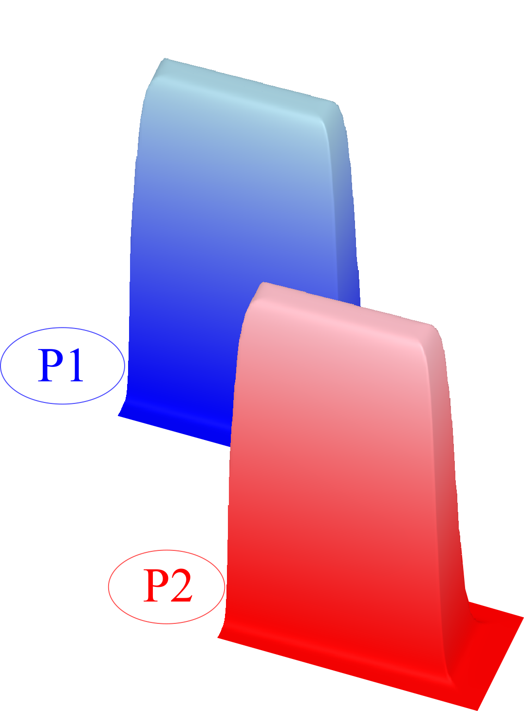
Figure 3: Longitudinal acceleration limits in the draft region behind a player visualized as a surface, where the maximum height of the surface is $u_{\text{max}}^{\text{draft}}$.

$$g_{i}^{\text{accel}}(x)=\begin{bmatrix}u_{i}^{\text{lat}}+u_{\text{max}}^{\text{nom}}\\ u_{\text{max}}^{\text{nom}}-u_{i}^{\text{lat}}\\ u_{i}^{\text{long}}+u_{\text{max}}^{\text{brake}}\\ u_{\text{i, max}}^{\text{draft}}(y_{-i})-u_{i}^{\text{long}}\\ \end{bmatrix}\geq\mathbf{0}$$

The upper limit for the longitudinal acceleration of the $i$^th player $u_{\text{i, max}}^{\text{draft}}(y_{-i})$ is boosted in the smooth rectangular area behind the opposing player, and the value of the maximum draft acceleration is defined as the surface attached to the opposing player’s position as shown in Fig. 3 (The length and width of this drafting region is determined by the parameters $\ell_{\text{draft}},w_{\text{draft}}$). The drafting aspect of our racing model encourages close proximity interaction. Furthermore, to allow defensive strategies, we permit greater braking accelerations than the maximum possible forward acceleration with drafting.

V Simulations and Discussion

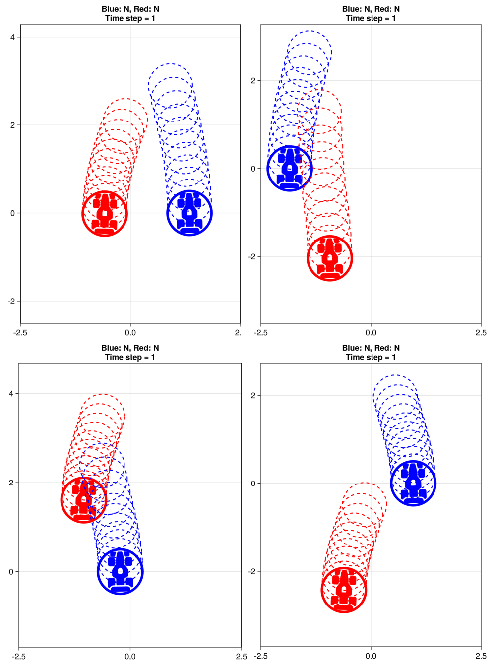
(a) P1 and P2 has agreed to the Nash competition.

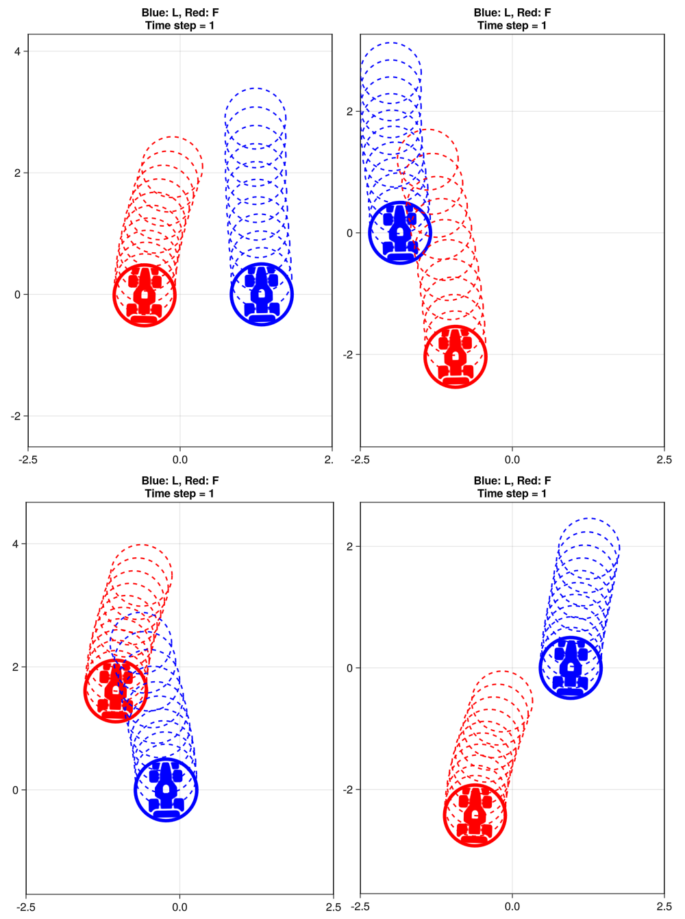
(b) P1 and P2 has agreed to the bilevel competition, and that P1 is the leader.

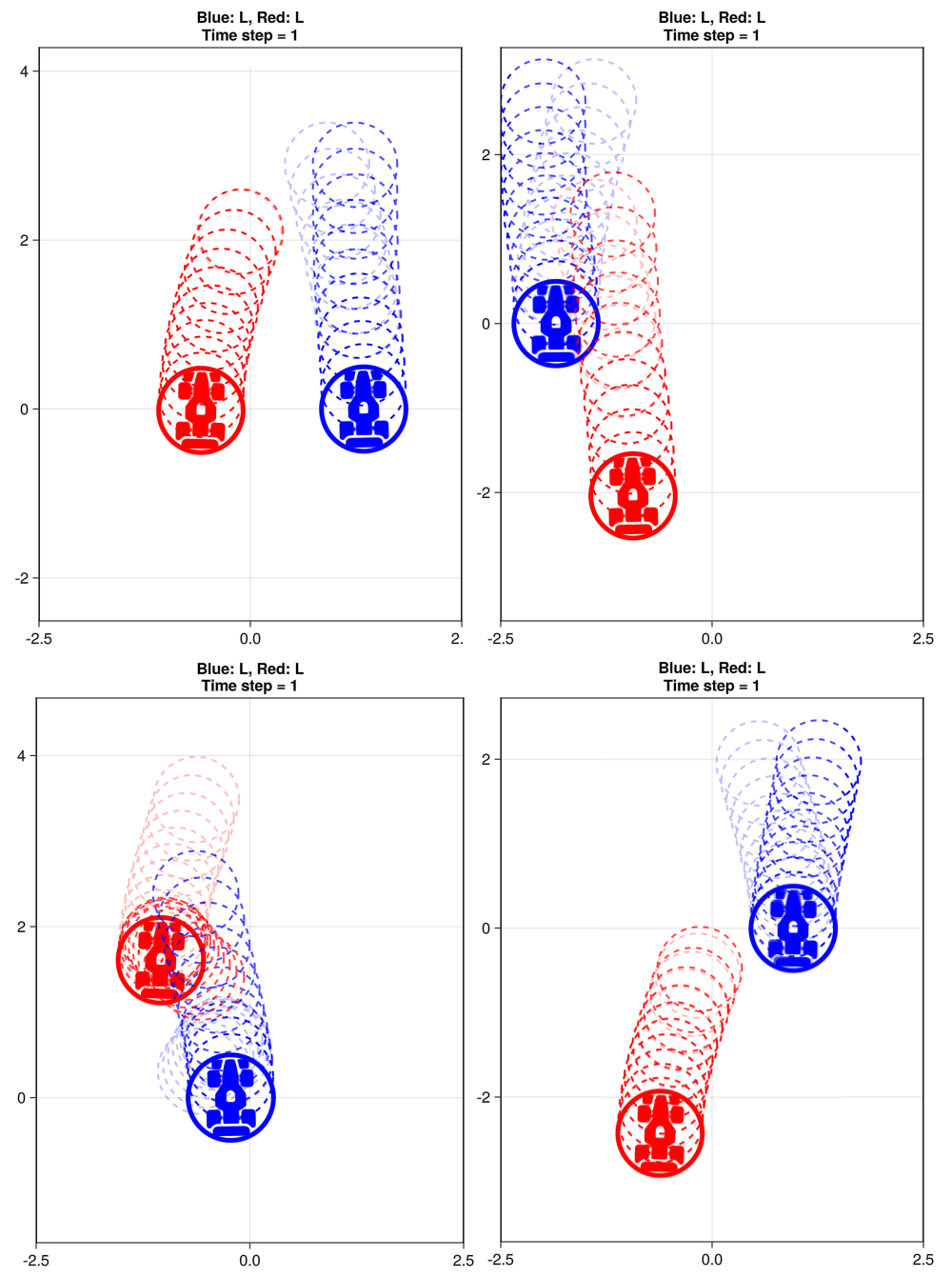
(c) P1 and P2 has agreed to the bilevel competition, but they incorrectly believe they are both the leader.

Figure 4: Four different initial conditions in three different competition types for P1 (Blue) and P2 (Red): (a) Nash competition, (b) bilevel competition, (c) bilevel competition with disagreement. When the players do not agree on the competition type as in sub-figure (c), we superimposed the opponent’s contradictory plan with transparency.

In this section we compare 16 different competition types as a combination of different information patterns using our two-player racing model that was detailed in Section IV using a large scale randomized simulation trial. In the distributed brain scenario, where the players do not have to agree on the information structure, each player can unilaterally choose from one of the four information patterns, without knowing what the other player will do. We enumerate the 16 different competition types that we investigate in this study in Table I. In Table I and the other tables that follow it, the columns represent Player 1’s assumed equilibrium type, while the rows represent Player 2’s assumed equilibrium type.

TABLE I: Competition types.

	SP (S)	Nash (N)	Leader (L)	Follower (F)
SP (S)	S-S	N-S	L-S	F-S
Nash (N)	S-N	N-N	L-N	F-N
Leader (L)	S-L	N-L	L-L	F-L
Follower (F)	S-F	N-F	L-F	F-F

Due to the symmetry in the information patterns, we only have to compute 10 different competition types for each initial condition in order to fill this table, which we arbitrarily chose as the lower-triangular section of Table I, including the diagonal.

For each competition type we have simulated 2000 randomly generated feasible initial conditions for 50 time steps, using $n_{T}=10$ number computation horizon time steps. The other parameters of our model and simulation are listed in Table II When we generated the random initial conditions, we first chose the first player’s lateral position from a uniform distribution between the lateral road limits. Then, the second player’s position was chosen from a uniform radial distribution of minimum and maximum radius based on the desired minimum collision radius, and if necessary it was resampled to remain within the lateral road limits. Then for the initial velocities, the first player’s longitudinal velocity is sampled from a uniform non-negative range, while the second player’s longitudinal velocity is computed as a uniformly distributed offset compared to the first player’s velocity. The initial lateral velocities were kept at zero.

We showcase a small sample of initial conditions and the first time step motion plans that correspond to different competition types in Fig. 4. In Fig. 4 (c), we overlay the realized simulation and the mistaken expectations of the players, where the transparent plans correspond to each player’s incorrect expectation that the opponent will play as a follower, e.g. the transparent Red trajectory is what Blue thinks Red would do as a follower, and vice versa.

TABLE II: Simulation and game parameters.

Parameter	Value	Parameter	Value
$\alpha_{1}$	$1\text{\times}{10}^{-3}$	$u_{\text{max}}^{\text{nom}}$	1.0^-2
$\alpha_{2}$	$1\text{\times}{10}^{-4}$	$u_{\text{max}}^{\text{brake}}$	5.0^-2
$\beta$	$1\text{\times}{10}^{-1}$	$u_{\text{max}}^{\text{draft}}$	2.5^-2
$n_{T}$	$10$	$y_{\text{min}}^{\text{lat}}$	-2.
$\Delta t$	1e-1	$y_{\text{max}}^{\text{lat}}$	2.
$r_{\text{desired}}$	1.2	$\dot{y}_{1,0,\text{min}}^{\text{long}}$	1.5^-1
$c_{d}$	.2^-1	$\dot{y}_{1,0,\text{max}}^{\text{long}}$	3.0^-1
$r$	1.0	$\dot{y}_{2,0,\Delta}^{\text{long}}$	1.5^-1
$\ell_{\text{draft}}$	5.0	$w_{\text{draft}}$	2.0

Solving bilevel problems poses a significant challenge due to their sensitivity to initialization of the solver. Depending on the initialization, the solver can get stuck in a disadvantageous local equilibrium points or fail to find an equilibrium. Because of this, we follow a fallback strategy when we are solving for the bilevel equilibrium. We initialize the bilevel solver using the Nash equilibrium solution, in the event that the solver fails to reach an equilibrium, we fall back to using the single-player solution as our initialization. In the case this all fails, we fall back to an uncontrolled simulation step in the hopes that the situation may improve in the subsequent iterations. Most importantly, at the start of every simulation step, we manually check all constraints. If the initial position and velocities of the players violate the constraints such as the lateral road limits or the spatial collision constraints, we terminate the simulation on the basis of safety constraint violation.

V-A Robustness

Our metric for robustness is the mean number of steps of the simulation before the simulation is terminated due to one of the safety constraint violation scenarios: (i) One of the players was forced out of the road, or (ii) the players found themselves in an unavoidable player-to-player collision. We compile the results in Table III for all competition types.

Our results indicate that there is no significant difference in safety between the baseline single-player and Nash equilibrium competitions. However, this is not true for the bilevel competition. Playing as a leader causes increased competitive behavior on the part of the ego player, however this increased aggression is reflected as decreased safety. On the other hand, we observe that playing as a follower leads to decreased aggression and therefore increased safety. Independent of what the opponent does, the most dangerous strategy for the ego player is to assume that they are the leader. Similarly, the safest strategy for the ego player is to assume that they are the follower.

TABLE III: Mean number of simulation steps before safety constraint violation for different combination of competition types, within the 95% confidence interval.

	SP (S)	Nash (N)	Leader (L)	Follower (F)
SP (S)	$45.0\pm 0.5$	$39.6\pm 0.6$	$30.8\pm 0.7$	$42.1\pm 0.6$
Nash (N)	$39.6\pm 0.6$	$39.8\pm 0.6$	$29.4\pm 0.7$	$44.3\pm 0.5$
Leader (L)	$30.8\pm 0.7$	$29.4\pm 0.7$	$21.0\pm 0.6$	$34.5\pm 0.7$
Follower (F)	$42.1\pm 0.6$	$44.3\pm 0.5$	$34.5\pm 0.7$	$47.5\pm 0.4$
Average	$39.4\pm 0.3$	$38.3\pm 0.4$	$28.9\pm 0.5$	$42.1\pm 0.3$

We observe that the leader-leader competition leads to the lowest mean number of simulation steps before termination. We stipulate this is due to the players having a false sense of confidence about their ability to enforce their strategies on their opponent. This situation naturally leads to increased rates of collision, and the worst case scenario occurs when both players incorrectly believe that they are the leader in a bilevel game. Furthermore, the Follower-Follower scenario scores highest in terms of mean time steps before safety constraint violation. In this section we have shown that the mean number of simulation steps before a safety violation depends significantly on the competition type.

V-B Performance

In this section we compare the performance of different competition types and we use the mean running cost as our metric for competitive advantage. In Fig. 5, we plot the average cost per time step for Nash and bilevel competition information patterns with respect to simulation steps. We observe that the most competitive behavior occurs at the beginning of the simulation, and most of the interaction concludes after about 20 simulation steps. We display the statistical distribution of mean running cost per step for the Nash and bilevel competitions in Fig. 6, which corresponds to each line in Fig. 5. Unsurprisingly, single-player and Nash competition leads to an average cost of zero within the confidence limit, while the bilevel competition leads to decreased cost for the ego player who is playing as the leader.

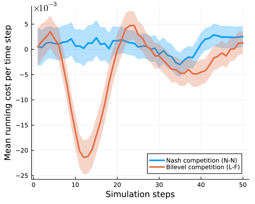
Figure 5: Mean running costs for the ego player when both players agree on Nash equilibrium (N-N) or bilevel (L-F) competition type with respect to all initial conditions and time steps. The shaded area is the 95% confidence interval.

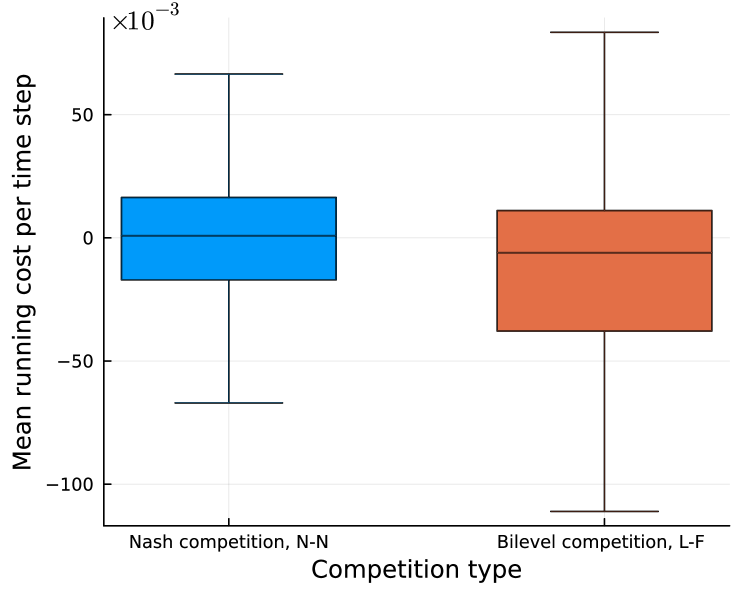
Figure 6: Mean running cost compared with respect to different competition types. (Whiskers of the box plot corresponds to the $1.5\mathrm{IQR}$.)

TABLE IV: Mean running costs of different combinations of competition types for the ego player, P1, within the 95% confidence interval.

$10^{-3}$	S	N	L	F
S	$1.75\pm 1.22$	$0.83\pm 1.43$	$-11.50\pm 0.22$	$7.84\pm 1.28$
N	$0.82\pm 0.14$	$0.24\pm 1.47$	$-8.06\pm 2.06$	$9.38\pm 1.15$
L	$13.50\pm 0.23$	$10.20\pm 0.21$	$1.24\pm 2.54$	$17.30\pm 0.18$
F	$-6.33\pm 1.28$	$-7.88\pm 1.14$	$-15.40\pm 0.18$	$0.92\pm 0.90$
Avg.	$2.43\pm 1.27$	$0.85\pm 0.76$	$-8.42\pm 0.88$	$8.86\pm 0.76$

We compile the performance of the ego player for different competition types in Table IV. If both players that agree Nash competition, there is no competitive advantage to be exploited by either player, and the baseline single-player results are similar to the Nash competition. On the other hand, bilevel competition leads Playing leader against an opponent that plays follower provides the best competitive advantage, while the difference between playing single-player and Nash equilibrium is negligible.

We observe that the bilevel competition leads to increased competitive advantage to the leader, which is reflected as disadvantage to the follower. Assuming to play as the follower comes at a cost penalty even against an opponent who is thinks the game that is played in single-player or Nash competition. The competitive advantage comes with increased collision risk and therefore reduced safety as we have discussed in the previous section, especially if both players greedily assume that they are the leader, the likelihood of a collision or road limit violation increases significantly. On the other hand, it is always a safe choice to assume for the players to assume that they are a follower unilaterally, but it can be exploited by a risk-taking opponent.

VI Conclusion

In this study we performed a large scale empirical analysis on the benefits felt from computing trajectories via bilevel competition compared to static reasoning. We have shown that the information structure has a significant effect on the competitive performance and safety. We observed that bilevel reasoning can lead to competitive advantage in the physical racing domain, but it is potentially a trade-off with safety if the players do not agree on the competition type.

When players act greedy and find themselves in Leader-Leader competition, the result is decreased safety for all players. On the flip side, bilevel competition as an always-follower can lead to increased safety for all players, but at the cost of sacrificing some competitive performance. We have shown that the mean number of simulation steps before safety constraint violations depend significantly on the information pattern. Relative preference between high competitive performance and high safety could guide leader or follower preference in bilevel competition. In the future we plan to explore other advanced information patterns in noncooperative dynamic games.

References

- Arrow and Debreu [1954] Kenneth J Arrow and Gerard Debreu. Existence of an equilibrium for a competitive economy. Econometrica: Journal of the Econometric Society, pages 265–290, 1954.
- Burger et al. [2022] Christoph Burger, Johannes Fischer, Frank Bieder, Omer Sahin Tas, and Christoph Stiller. Interaction-Aware Game-Theoretic Motion Planning for Automated Vehicles using Bi-level Optimization. In 2022 IEEE 25th International Conference on Intelligent Transportation Systems (ITSC), pages 3978–3985, Macau, China, October 2022. IEEE. ISBN 978-1-66546-880-0. doi: 10.1109/ITSC55140.2022.9922600. URL https://ieeexplore.ieee.org/document/9922600/.
- Cournot [1927] Antoine Augustin Cournot. Researches into the Mathematical Principles of the Theory of Wealth. New York: Macmillan Company, 1927 [c1897], 1927.
- Daughety [1990] Andrew F Daughety. Beneficial concentration. The American Economic Review, 80(5):1231–1237, 1990.
- Debreu [1952] Gerard Debreu. A social equilibrium existence theorem. Proceedings of the National Academy of Sciences, 38(10):886–893, 1952.
- Dirkse and Ferris [1995] Steven P Dirkse and Michael C Ferris. The path solver: a nommonotone stabilization scheme for mixed complementarity problems. Optimization methods and software, 5(2):123–156, 1995.
- Facchinei and Kanzow [2007] Francisco Facchinei and Christian Kanzow. Generalized nash equilibrium problems. 4or, 5:173–210, 2007.
- Facchinei and Pang [2003] Francisco Facchinei and Jong-Shi Pang. Finite-dimensional variational inequalities and complementarity problems. Springer, 2003.
- Fridovich-Keil et al. [2020] David Fridovich-Keil, Ellis Ratner, Lasse Peters, Anca D Dragan, and Claire J Tomlin. Efficient iterative linear-quadratic approximations for nonlinear multi-player general-sum differential games. In 2020 IEEE international conference on robotics and automation (ICRA), pages 1475–1481. IEEE, 2020.
- Hu and Fukushima [2015] Ming Hu and Masao Fukushima. Multi-Leader-Follower Games: Models, Methods and Applications. Journal of the Operations Research Society of Japan, 58(1):1–23, 2015. ISSN 0453-4514, 2188-8299. doi: 10.15807/jorsj.58.1. URL https://www.jstage.jst.go.jp/article/jorsj/58/1/58_1/_article. Number: 1.
- Huck et al. [2001] Steffen Huck, Wieland Muller, and Hans-Theo Normann. Stackelberg beats cournot—on collusion and efficiency in experimental markets. The Economic Journal, 111(474):749–765, 2001.
- Ji et al. [2021] Kyoungtae Ji, Matko Orsag, and Kyoungseok Han. Lane-Merging Strategy for a Self-Driving Car in Dense Traffic Using the Stackelberg Game Approach. Electronics, 10(8):894, January 2021. ISSN 2079-9292. doi: 10.3390/electronics10080894. URL https://www.mdpi.com/2079-9292/10/8/894. Number: 8 Publisher: Multidisciplinary Digital Publishing Institute.
- Karush [1939] William Karush. Minima of functions of several variables with inequalities as side constraints. M. Sc. Dissertation. Dept. of Mathematics, Univ. of Chicago, 1939.
- [14] H Kuhn. Tucker (1951). nonlinear programming. In Proceedings of the second Berkeley symposium on mathematical statistics and probability, Berkeley, University of California, pages 481–492.
- Laine et al. [2021] Forrest Laine, David Fridovich-Keil, Chih-Yuan Chiu, and Claire Tomlin. Multi-hypothesis interactions in game-theoretic motion planning. In 2021 IEEE International Conference on Robotics and Automation (ICRA), pages 8016–8023. IEEE, 2021.
- Laine et al. [2023] Forrest Laine, David Fridovich-Keil, Chih-Yuan Chiu, and Claire Tomlin. The computation of approximate generalized feedback nash equilibria. SIAM Journal on Optimization, 33(1):294–318, 2023.
- Le Cleac’h et al. [2022] Simon Le Cleac’h, Mac Schwager, and Zachary Manchester. Algames: a fast augmented lagrangian solver for constrained dynamic games. Autonomous Robots, 46(1):201–215, 2022.
- Liniger and Lygeros [2020] Alexander Liniger and John Lygeros. A Noncooperative Game Approach to Autonomous Racing. IEEE transactions on control systems technology, 28(3):884–897, 2020. ISSN 1063-6536. doi: 10.1109/TCST.2019.2895282. Publisher: IEEE.
- Nash [1951] John Nash. Non-cooperative games. Annals of mathematics, pages 286–295, 1951.
- Von Stackelberg [2010] Heinrich Von Stackelberg. Market structure and equilibrium. Springer Science & Business Media, 2010.