Layerwise Proximal Replay: A Proximal Point Method
for Online Continual Learning

Abstract

In online continual learning, a neural network incrementally learns from a non-i.i.d. data stream. Nearly all online continual learning methods employ experience replay to simultaneously prevent catastrophic forgetting and underfitting on past data. Our work demonstrates a limitation of this approach: networks trained with experience replay tend to have unstable optimization trajectories, impeding their overall accuracy. Surprisingly, these instabilities persist even when the replay buffer stores all previous training examples, suggesting that this issue is orthogonal to catastrophic forgetting. We minimize these instabilities through a simple modification of the optimization geometry. Our solution, Layerwise Proximal Replay (LPR), balances learning from new and replay data while only allowing for gradual changes in the hidden activation of past data. We demonstrate that LPR consistently improves replay-based online continual learning methods across multiple problem settings, regardless of the amount of available replay memory.

1 Introduction

Continual learning is a subfield of machine learning that studies how to enable models to continuously adapt to new information over time without forgetting old information under memory and computation constraints. Online continual learning is a particularly challenging form of continual learning where a neural network must learn from a non-stationary data stream. Data arrive in small batches, typically between $1$ to $10$ data points, and the network can typically only train for a few iterations before the next batch arrives.

Almost all successful approaches to online continual learning rely on replay buffers (Soutif-Cormerais et al., 2023), or small subsets of prior data used during training to approximate the loss over all past data. Replay-based approaches are particularly dominant in online continual learning for two reasons. First, training on prior data helps to prevent catastrophic forgetting (French, 1999), arguably the primary bottleneck in continual learning. Second, replay increases the overall number of training iterations where the network is exposed to past data. This is especially crucial in the online setting, which is otherwise prone to underfitting due to the rapid arrival of new data (Zhang et al., 2022).

Despite their proven ability to mitigate catastrophic forgetting and underfitting, we hypothesize that online replay methods are inefficient from an optimization perspective. At any given training iteration, the new data batch and replay data both contribute to the overall training loss. However, since the network has already trained to some extent on replay data, new data will likely contribute more to the overall training loss. The resulting parameter updates will bias the network toward the new data and potentially causing the network to forget useful representations for prior data, at times severely (De Lange et al., 2022). Although past data performance can be partially recovered after additional training on replay examples, overall representational instability is wasteful and can slow optimization and affect predictive performance.

In this work, we tackle these inefficiencies through a simple optimizer modification, which maintains the advantages of replay-based continual learning while improving its stability. Our method, which we refer to as Layerwise Proximal Replay (LPR), applies a replay-tailored preconditioner to the loss gradients, builds upon a growing literature of continual learning methods that modify the gradient update geometry (Chaudhry et al., 2018; Zeng et al., 2019; Kao et al., 2021; Saha et al., 2021b; Saha & Roy, 2023). LPR’s preconditioners balance two desiderata: 1. maximally learning from both new and past data while 2. only gradually changing past data predictions (and internal representations) to promote optimization stability and convergence.

Across several predictive tasks and datasets, we find that LPR consistently improves upon the accuracy of replay-based online continual learning methods. Importantly, LPR achieves performance gains that are robust to the choice of replay loss as well as the size of the replay buffer. We even notice substantial performance gains when the replay buffer has unlimited memory and thus is able to “remember” all data encountered during training. These results suggest that LPR can improve performance even when the catastrophic forgetting problem is largely mitigated.

To summarize, we make the following contributions:

1. We introduce Layerwise Proximal Replay (LPR), the first online continual learning method that combines experience replay with proximal optimization.

2. We demonstrate through extensive experimentation that LPR consistently improves state-of-the-art online continual learning methods across problem settings and replay buffer sizes.

3. We analyze the effects of LPR, demonstrating improved optimization and fewer destabilizing changes to the network’s hidden representations.

2 Background

Notation.

Given an $L$-layer neural network, we will denote a specific layer’s parameters as the matrix $\Theta^{(\ell)}$, where $\ell$ is the layer index. For linear layers, $\Theta^{(\ell)}$ is a $d^{\ell}\times d^{\ell+1}$ matrix, where $d^{\ell}$ is the dimensionality of layer $\ell$’s hidden representation. The vector $\theta$ will refer to the concatenation of all of the (flattened) network parameters—i.e. $\theta=\begin{bmatrix}\mathrm{vec}(\Theta^{(1)})&\ldots&\mathrm{vec}(\Theta^{(L)})\end{bmatrix}$.

Online continual learning

is a problem setup where a model incrementally learns from a potentially non-i.i.d. data stream in a memory and/or computation limited setting. In the classification setting, at time $\tau$ the neural network receives a data batch $\mathcal{D}_{\tau}=\{X_{\tau,i},Y_{\tau,i}\}_{i=1}^{n_{\tau}}$ with $n_{\tau}$ features and labels. We assume that we are in the classification setting and that $n_{\tau}$ is equal for all data batches for the rest of the paper. Once the neural network trains on a data batch, it cannot train on the same batch again aside from a small sample of it that may be present in a replay buffer.

In the online continual learning literature, the data stream is often built from a sequence of “tasks”, where each task is defined by a dataset a model should train on. The data stream is built as follows. Initially, each task’s dataset is split into mutually exclusive data batches of much smaller size that are i.i.d. sampled without replacement. Then, a data stream is constructed such that it sequentially returns all data batches from the first task, then all data batches from the second task, and so forth.

Online continual learning is distinct from offline continual learning in a number of ways (Soutif-Cormerais et al., 2023). Typically, $n_{\tau}$ is much smaller than offline continual learning, falling in between 1 and 100. In addition, if the data stream is characterized by a sequence of tasks (a problem accompanied by a dataset) where data batches that belong to a single tasks arrive in an i.i.d. fashion, the task boundary is usually not provided. Lastly, models must perform well at any point of their training, unlike offline continual learning models where evaluation is performed every time when the models finish training on a task.

In practice, models underfit the data stream in online continual learning (Zhang et al., 2022) because they can only train on each data batch’s datapoints once, aside from a small number of past datapoints that may be kept in a replay buffer. To clarify, the model may take multiple contiguous gradient steps for the new data batch, but it may no longer be trained on the same data batch afterward.

Replay methods

are employed in both offline and online continual learning, but they are especially dominant in the latter (Soutif-Cormerais et al., 2023). At time $\tau$, replay methods loosely approximate the loss over all previously observed data batches with

$$\mathcal{L}(\theta)\coloneqq\mathcal{L}_{\mathrm{new}}(\theta,\mathcal{D}_{\tau})+\alpha\mathcal{L}_{\mathrm{replay}}(\theta,\mathcal{M})$$ (1)

where $\theta$ is the vector of network parameters, $\mathcal{M}$ is either a much smaller subset of past data batches or pseudo datapoints that summarize the past data, $\alpha$ is the replay regularization strength, and $\mathcal{L}_{\mathrm{replay}}(\theta,\mathcal{M})$ is the loss associated with the replay buffer.

Proximal point methods

(Drusvyatskiy, 2017; Parikh & Boyd, 2014; Asi & Duchi, 2019) are optimization algorithms that minimize a function $\mathcal{L}(\theta)$ by repeated application of the $\mathrm{prox}$ operator:

$$\theta_{j+1} =\mathrm{prox}_{\eta\mathcal{L}}\left(\theta_{j}\right),$$ (2)

$$\mathrm{prox}_{\eta\mathcal{L}}\left(\theta_{j}\right) :=\operatorname*{arg\,min}_{\theta}\left[\mathcal{L}(\theta)+\tfrac{1}{2\eta}\|\theta-\theta_{j}\|^{2}\right].$$

Here, $\theta_{j}$ is the model parameter value at $j$-th optimization iteration, $\|\cdot\|$ is some norm that satisfies the parallelogram identity, and $\eta^{-1}$ is the proximal penalty strength. For many functions, solving Equation 2 can be as hard as solving the original minimization objective. Therefore, it is common to make approximations such as linearization of $\mathcal{L}$ around $\theta_{j}$. Notably, gradient descent can be cast as a proximal point method by linearizing $\mathcal{L}$ and using the Euclidean norm.

3 Layerwise Proximal Replay

Motivation.

We have three desiderata for replay-based online continual learning: 1. the network should rapidly learn from new data batches, 2. the network should continue learning from prior (replay) data, and 3. parameter updates should not cause sudden unnecessary performance degradation on the past data, thus ensuring stable optimization while preventing underfitting. We hypothesize that existing online replay methods largely ignore the third, resulting in inefficient optimization that ultimately harms accuracy.

We can instead satisfy all three desiderata by modifying the optimizer on top of experience replay. Consider the standard SGD update $\theta_{j+1}=\theta_{j}-\eta\nabla\mathcal{L}(\theta_{j})$. This update naturally codifies the first two desiderata, as $\mathcal{L}(\theta_{j})$ combines both the new data and replay data losses. To encode the third, we simply constrain the optimizer to only consider updates that minimally change replay predictions.

Consider the proximal formulation of SGD (e.g. Parikh & Boyd, 2014):

$$\theta_{j+1} =\mathrm{prox}_{\eta\mathcal{L}}\left(\theta_{j}\right):=\operatorname*{arg\,min}_{\theta}\left(\mathcal{L}(\theta)+\tfrac{1}{2\eta}\|\theta-\theta_{j}\|^{2}_{2}\right)$$

$$\approx\operatorname*{arg\,min}_{\theta}\left(\left\langle\nabla\mathcal{L}(\theta_{j}),\theta\!-\!\theta_{j}\right\rangle+\tfrac{1}{2\eta}\|\theta-\theta_{j}\|^{2}_{2}\right)$$ (3)

$$=\theta_{j}-\eta\nabla\mathcal{L}(\theta_{j})$$

where Equation 3 uses first order Taylor approximation $\mathcal{L}(\theta)-\mathcal{L}(\theta_{j})\approx\left\langle\nabla\mathcal{L}(\theta_{j}),\theta-\theta_{j}\right\rangle$. Intuitively, the norm penalty on $\theta-\theta_{j}$ ensures that the update only considers values of $\theta$ where the Taylor approximation is reasonable. We can further restrict the search space to updates that minimally change replay predictions by modifying Equation 3 as follows:

$$\operatorname*{arg\,min}_{\theta}\left(\langle\nabla\mathcal{L}(\theta_{j}),\theta-\theta_{j}\rangle+\tfrac{1}{2\eta}\|\theta-\theta_{j}\|^{2}_{2}\right),$$ (4)

$$\mathrm{s.t.}\ \|F(\theta)-F(\theta_{j})\|_{2}^{2}<\delta.$$

Here, $\delta>0$ is some hyperparameter and $F(\theta)\in\mathbb{R}^{|\mathcal{M}|\times c}$ is the matrix of predictions for all replay data given neural network parameters $\theta$.

Layerwise Proximal Replay.

In practice, it is challenging to implement this functional constraint efficiently in online continual learning. To that end, we instead consider the stronger constraint of ensuring a minimal change to the hidden activations of replay data:

$$\operatorname*{arg\,min}_{\theta}\left(\left\langle\nabla\mathcal{L}(\theta_{j}),\theta-\theta_{j}\right\rangle+\tfrac{1}{2\eta}\|\theta-\theta_{j}\|^{2}_{2}\right),$$ (5)

$$\mathrm{s.t.}\ \|Z^{(\ell)}(\theta)-Z^{(\ell)}(\theta_{j})\|_{F}^{2}<\delta^{(\ell)},\>\>\ell\in\{1,\ldots,L\}$$

where $Z^{(\ell)}(\theta)\in\mathbb{R}^{|\mathcal{M}|\times d^{\ell}}$ is the matrix of $\ell$-th layer activations for all replay data, $\delta^{(\ell)}>0$ are some layerwise constraint constants, and $\|\cdot\|_{F}$ is the Frobenius norm. We can approximately apply this constraint in a layer-wise fashion. Let $\Theta^{(i)}\in\mathbb{R}^{d^{\ell}\times d^{\ell+1}}$ be the matrix of parameters at layer $\ell$, and let $Z^{(\ell)}_{j}\in\mathbb{R}^{|\mathcal{M}|\times d^{\ell}}$ be the hidden activations for layer $\ell$ at time $j$. The activations follow the recursive formula $Z^{(\ell+1)}_{j}=\phi^{(\ell)}(Z^{(\ell)}_{j}\Theta^{(\ell)}_{j})$ where $\phi^{(\ell)}$ is the $l$-th layer’s activation function. If our parameter update minimally changes layer $\ell$’s activations (i.e. $Z^{(\ell)}_{j+1}\approx Z^{(\ell)}_{j}$), we can rewrite the constraint in Equation 4 as

$$\|Z^{(\ell)}_{j}\Theta^{(\ell)}_{j+1}-Z^{(\ell)}_{j}\Theta^{(\ell)}_{j}\|_{F}^{2}<\delta^{(\ell)}.$$

Applying a Lagrange multiplier to transform Equation 5, we have

$$\operatorname*{arg\,min}_{\theta}\big{(} \left\langle\nabla\mathcal{L}(\theta_{j}),\theta-\theta_{j}\right\rangle+\tfrac{1}{2\eta}\|\theta-\theta_{j}\|^{2}_{2}$$ (6)

$$+{\textstyle\sum_{\ell=1}^{L}}\lambda^{(\ell)}\|Z^{(\ell)}_{j}\Theta^{(\ell)}_{j+1}-Z^{(\ell)}_{j}\Theta^{(\ell)}_{j}\|_{F}^{2}\big{)}.$$

This can in turn be converted to a layer-wise update rule

$$\Theta^{(\ell)}_{j+1}\! =\!\operatorname*{arg\,min}_{\Theta^{(\ell)}}\!\bigg{(}\!\left\langle\nabla\mathcal{L}(\Theta_{j}^{(\ell)}),\Theta^{(\ell)}\!\!-\!\Theta_{j}^{(\ell)\!}\right\rangle\!$$ (7)

$$\quad\quad\quad\quad\quad+\!\tfrac{1}{2\eta}\|\Theta^{(\ell)}\!\!-\!\Theta^{(\ell)}_{j}\!\|^{2}_{P_{\ell}}\bigg{)}$$

$$=\!\Theta_{j}^{(\ell)}-\eta P_{\ell}^{-1}\nabla L(\Theta_{j}^{(\ell)}),$$ (8)

where $P_{\ell}$ is a positive definite matrix given by

$$P_{\ell}:=I+\omega^{\ell}Z^{(\ell)^{\top}}_{j}Z^{(\ell)}_{j},$$ (9)

$\omega^{\ell}=2\eta\lambda^{(\ell)}$ is a hyperparameter that absorbs the Lagrange multiplier $\lambda^{(\ell)}$, $\nabla L(\Theta_{j}^{(\ell)})$ is a shorthand for $\nabla_{\Theta^{(\ell)}}\mathcal{L}(\theta_{j})$, and $\|\cdot\|_{P_{\ell}}$ is the norm given by $\sqrt{\mathrm{tr}\left((\cdot)^{\top}P_{\ell}(\cdot)\right)}$ (See Appendix A for the derivation.)

Note that Equation 8, like Equation 3, can be construed as an application of the $\mathrm{prox}$ operator, but here the proximity function is given by the layerwise $P_{\ell}$-norm rather than the standard Euclidean norm. The use of this non-Euclidean proximal update in conjunction with the replay loss ensures continued learning while simultaneously limiting sudden degradations in replay performance. We refer to Equation 8 as Layerwise Proximal Replay, or LPR for short.

Algorithm 1 Layerwise Proximal Replay (LPR)

  Input: network parameters $\theta$, learning rate $\eta$, per batch gradient steps count $S$, preconditioner update interval $T$, layerwise stability hyperparameters $\omega_{0}^{\ell}$ for $\ell\in\{1,...,L\}$.

  Output: trained network parameters $\theta$.

  Initialize replay buffer: $\mathcal{M}\leftarrow\{\}$.

  Initialize preconditioner inverses $\Lambda_{\ell}\leftarrow I,\ \ell\in\{1,...,L\}$. {$\Lambda_{\ell}=P_{\ell}^{-1}$}

  for $\tau\in\{1,...,\infty\}$ do

     Obtain new data batch $\mathcal{D}_{\tau}$.

     for $s\in\{1,...,S\}$ do

        Compute loss $\mathcal{L}(\theta)$ using $\mathcal{D}_{\tau}$ and $\mathcal{M}$.

        Compute loss gradient $\nabla\mathcal{L}(\theta)$.

        for layer index $\ell\in\{1,...,L\}$ do

           $\Theta^{(\ell)}\leftarrow\Theta^{(\ell)}-\eta\Lambda_{\ell}\nabla_{\Theta^{(\ell)}}\mathcal{L}(\theta)$ {$\Lambda_{\ell}=P_{\ell}^{-1}$}

        end for

     end for

     Update $\mathcal{M}$ with $\mathcal{D}_{\tau}$.

     if $\tau\bmod{T}=0$ then

        Obtain feature tensor $X_{mem}$ from $\mathcal{M}$.

        Set $Z^{(1)}$ to $X_{mem}$ and $n$ to the batch size of $X_{mem}$.

        for layer index $\ell\in\{1,...,L\}$ do

           $\omega^{\ell}\leftarrow\omega_{0}^{\ell}/n$

           $\Lambda_{\ell}\leftarrow\left(\omega^{\ell}{Z^{(\ell)}}^{\mkern-6.0mu\top}Z^{(\ell)}+I\right)^{-1}$ {$\Lambda_{\ell}=P_{\ell}^{-1}$}

           $Z^{(\ell+1)}\leftarrow\phi^{(\ell)}(Z^{(\ell)}\Theta^{(\ell)})$

        end for

     end if

  end for

Analysis.

LPR can be viewed as a variant of preconditioned SGD where the symmetric positive definite preconditioner $P_{\ell}$ is specific to each layer. We note that setting $\omega^{\ell}=0$ recovers the standard SGD update. When $\omega^{\ell}>0$, the eigenvalues of $P_{\ell}$ are all greater than 1, and thus $P_{\ell}^{-1}$ is a contraction operator; i.e.

$$\|P_{\ell}^{-1}\nabla\mathcal{L}(\Theta_{j}^{(\ell)})\|_{F}<\|\nabla\mathcal{L}(\Theta_{j}^{(\ell)})\|_{F}.$$

Crucially, this contraction is not a simple rescaling of the gradient contributions from new data. Intuitively, we have $\|P_{\ell}^{-1}\nabla\mathcal{L}(\Theta_{j}^{(\ell)})\|_{F}\ll\|\nabla\mathcal{L}(\Theta_{j}^{(\ell)})\|_{F}$ when the standard gradient update would significantly alter replay predictions, and $\|P_{\ell}^{-1}\nabla\mathcal{L}(\Theta_{j}^{(\ell)})\|_{F}<\|\nabla\mathcal{L}(\Theta_{j}^{(\ell)})\|_{F}$ otherwise.

Implementation.

Algorithm 1 illustrates LPR in detail. The hyperparameter $S$ and $T$ specifies how many gradient steps to take per incoming data batch and the interval at which $P_{\ell}$ is recomputed from $\mathcal{M}$ for computational purposes respectively. Algorithmically, we store our preconditioner as $\Lambda_{\ell}:=P_{\ell}^{-1}$ so that each application of the preconditioner does not require performing matrix inversion.

In practice, specifying the hyperparameters $\omega_{0}^{\ell}$ for each layer can be cumbersome, especially for large neural networks. Therefore, in our experiments we parameterize $\omega_{0}^{\ell}$ for all layers using two scalar values $\omega_{0},\beta$ (refer to Appendix D).

In online continual learning, optimal hidden activations for past data are subject to change when additional relevant observations arrive from the data stream. Thus, LPR periodically refreshes $P_{\ell}$ with the current neural network’s feed-forward activations of the replay buffer inputs $X_{mem}$ from $\mathcal{M}$. For neural network layers that are not linear layers but can be cast as linear transformations, for example convolution and batch normalization, the input activation $Z^{(\ell)}$ is reshaped to allow it to be matrix multiplied with the layer’s weight matrix $\Theta^{(\ell)}$ for computing the layer’s output.

Compared to regular experience replay, LPR requires one additional matrix multiplication per layer for preconditioning the layer’s gradient per gradient step. In addition, once every $T$ data batches, it must feed forward replay buffer data through the network and invert $d^{\ell}\times d^{\ell}$ matrices per layer. The only memory requirement on top of regular experience replay is keeping $L$ preconditioners $P_{\ell}$.

Relation to projection-based continual learning.

Our method adds to a growing body of continual learning methods that apply transformations to the gradient updates (Chaudhry et al., 2018; Zeng et al., 2019; Farajtabar et al., 2020; Saha et al., 2021b; Kao et al., 2021; Deng et al., 2021; Shu et al., 2022; Guo et al., 2022; Saha & Roy, 2023). We offer a detailed review of these methods in Appendix C. Most gradient transformation methods have only been considered for offline learning (with (Chaudhry et al., 2018; Guo et al., 2022) being notable exceptions). Despite many surface level similarities, LPR differs from existing transformations in subtle but crucial ways necessary for replay-based online continual learning.

Our work is particularly related to those that construct the projection matrix such that the gradient updates occur approximately orthogonal to the subspace spanned by the past data’s hidden activations (Zeng et al., 2019; Saha et al., 2021b; Deng et al., 2021; Lin et al., 2022; Shu et al., 2022; Zhao et al., 2023; Saha & Roy, 2023). At a high level, these methods try to limit parameter updates to a $(d^{\ell}-k)$-dimensional subspace by applying an orthogonal projection to the gradients: $(I-\Phi^{(\ell)}(\Phi^{(\ell)^{\top}}\Phi^{(\ell)})^{-1}\Phi^{(\ell)^{\top}})\nabla\mathcal{L}(\Theta^{(\ell)})$, where the matrix $\Phi^{(\ell)}\in\mathbb{R}^{d^{\ell}\times k}$ defines the nullspace of the projection operator. Some work sets $\Phi^{(\ell)}$ to a low-rank approximation of all past-data activations computed in an SVD-like fashion (Saha et al., 2021b; Deng et al., 2021; Lin et al., 2022; Saha & Roy, 2023) while others average mini-batch activations to slowly build up $\Phi^{\ell}$ and not run out of capacity (Zeng et al., 2019; Guo et al., 2022). All methods structure the projection matrix such that gradient updates will preserve the high-level statistics of past-data representations as much as possible. See Appendix C for specifics of prior methods.

It is worth noting that projection operations (and their close approximations) are largely incompatible with continually learning from replay buffers. To see this, note that the matrix $(I-\Phi^{(\ell)}(\Phi^{(\ell)^{\top}}\Phi^{(\ell)})^{-1}\Phi^{(\ell)^{\top}})$ will project out any gradient contributions that from data points spanned by $\Phi^{(\ell)}$. (See Appendix B for a derivation.) If $\Phi^{(\ell)}$ approximately spans prior activations, then the replay loss will largely be projected out. Of course, $\Phi^{(\ell)}$ is too low dimensional to span all prior activations, and most practical methods use a “soft” approximation to the projection operator (Deng et al., 2021; Shu et al., 2022; Saha & Roy, 2023). Nevertheless, gradient projection methods largely minimize gradient information from the replay buffer, which is undesirable when we want to continue learning on past data.

LPR’s preconditioner has subtle but crucial differences that make it more compatible with online replay losses. Applying the Woodbury inversion formula to Equations 8 and 9, the LPR update can be written as

$$\left(I-Z^{(\ell)}\left(\tfrac{1}{\omega^{(\ell)}}I+Z^{(\ell)^{\top}}Z^{(\ell)}\right)^{-1}Z^{(\ell)^{\top}}\right)\nabla\mathcal{L}(\Theta^{(\ell)})$$ (10)

Note that we only recover a projection operator in the limiting case where 1. the replay buffer is really small (i.e. $|\mathcal{M}|<d^{\ell}$, so that $Z^{(\ell)}$ spans a subspace of $\mathbb{R}^{d^{\ell}}$) and 2. $\omega^{(\ell)}\to\infty$. Neither of these conditions is desirable for replay-based online continual learning. First, setting $\omega^{(\ell)}\to\infty$ would prevent any changes to replay data activations, which is undesirable in the online setting since networks are not trained to convergence before data are added to the replay buffer. We note that LPR with very high values of $\omega^{\ell}$ were never selected during our hyperparameter optimization (refer to Appendix E). Second, limiting $|\mathcal{M}|<d^{\ell}$ would severely harm performance, as prior work demonstrates that replay methods improve significantly as $|\mathcal{M}|$ gets larger. All together, LPR—unlike projection methods—enables further (albeit slower) learning on replay data and does not compress prior activations into low-rank approximations.

	Memory Size 1000			Memory Size 2000
Method	Acc	AAA	WC-Acc	Acc	AAA	WC-Acc
ER	0.2262 ± 0.0042	0.3255 ± 0.0055	0.1072 ± 0.0022	0.2937 ± 0.0054	0.3586 ± 0.0048	0.1264 ± 0.0030
LPR (ER)	0.2631 ± 0.0042	0.3782 ± 0.0059	0.1522 ± 0.0020	0.3334 ± 0.0056	0.4251 ± 0.0047	0.1926 ± 0.0026
DER	0.2339 ± 0.0045	0.3333 ± 0.0059	0.1178 ± 0.0035	0.2935 ± 0.0039	0.3575 ± 0.0073	0.1267 ± 0.0036
LPR (DER)	0.2634 ± 0.0036	0.3982 ± 0.0053	0.1700 ± 0.0029	0.3292 ± 0.0053	0.4325 ± 0.0059	0.2018 ± 0.0032
EMA	0.3124 ± 0.0061	0.3346 ± 0.0063	0.1078 ± 0.0029	0.3725 ± 0.0039	0.3665 ± 0.0050	0.1234 ± 0.0030
LPR (EMA)	0.3289 ± 0.0039	0.3783 ± 0.0063	0.1454 ± 0.0024	0.3884 ± 0.0029	0.4135 ± 0.0046	0.1755 ± 0.0032
LODE	0.2442 ± 0.0054	0.3391 ± 0.0068	0.1150 ± 0.0033	0.2969 ± 0.0033	0.3728 ± 0.0072	0.1346 ± 0.0036
LPR (LODE)	0.2740 ± 0.0051	0.3785 ± 0.0061	0.1753 ± 0.0054	0.3261 ± 0.0049	0.4102 ± 0.0058	0.2014 ± 0.0045

Table 1: Split-CIFAR100 results with mean and standard error computed across 10 random seeds.

	Memory Size 2000			Memory Size 4000
Method	Acc	AAA	WC-Acc	Acc	AAA	WC-Acc
ER	0.1590 ± 0.0016	0.2883 ± 0.0047	0.1016 ± 0.0016	0.2192 ± 0.0021	0.3368 ± 0.0044	0.1499 ± 0.0014
LPR (ER)	0.1669 ± 0.0014	0.2990 ± 0.0051	0.1134 ± 0.0010	0.2312 ± 0.0023	0.3492 ± 0.0042	0.1623 ± 0.0016
DER	0.1611 ± 0.0020	0.3010 ± 0.0041	0.1206 ± 0.0010	0.2294 ± 0.0019	0.3457 ± 0.0045	0.1685 ± 0.0016
LPR (DER)	0.1801 ± 0.0031	0.3121 ± 0.0047	0.1294 ± 0.0016	0.2408 ± 0.0032	0.3530 ± 0.0051	0.1751 ± 0.0013
EMA	0.1900 ± 0.0022	0.2870 ± 0.0040	0.1024 ± 0.0014	0.2603 ± 0.0017	0.3369 ± 0.0038	0.1506 ± 0.0013
LPR (EMA)	0.1959 ± 0.0018	0.3017 ± 0.0039	0.1128 ± 0.0013	0.2671 ± 0.0016	0.3504 ± 0.0039	0.1629 ± 0.0013
LODE	0.1978 ± 0.0022	0.3132 ± 0.0045	0.1351 ± 0.0015	0.2452 ± 0.0022	0.3522 ± 0.0041	0.1731 ± 0.0015
LPR (LODE)	0.1971 ± 0.0019	0.3170 ± 0.0044	0.1360 ± 0.0017	0.2518 ± 0.0015	0.3592 ± 0.0049	0.1799 ± 0.0015

Table 2: Split-TinyImageNet results with mean and standard error computed across 10 random seeds.

4 Experiments

In this section, we empirically investigate LPR’s effect on how a neural network learns during online continual learning. In addition, we extensively evaluate LPR across three online continual learning problems on top of four state-of-the-art experience replay methods. We will open-source the code upon acceptance.

4.1 Setup

Experiments.

We build on top of the Avalanche continual learning framework (Carta et al., 2023a) and closely follow the experiment setup from Soutif-Cormerais et al. (2023). We investigate LPR’s behavior and accuracy on two online class-incremental learning and one online domain-incremental learning problem settings (van de Ven et al., 2022). For online class-incremental learning, we evaluate on the online versions of Split-CIFAR100 and Split-TinyImageNet datasets (Soutif-Cormerais et al., 2023). Each dataset is divided and ordered into a sequence of 20 tasks that have mutually exclusive labels. These sequences are then converted to data streams where every data batch from the stream contains 10 datapoints that are i.i.d. sampled within tasks but not across tasks. For online domain-incremental learning, we evaluate on the online version of the CLEAR dataset (Lin et al., 2021). Domain-incremental learning involves adapting to sequentially changing data domains in real time. CLEAR’s built-in sequence of 10 tasks is converted to a data stream in the same manner as the online versions of Split-CIFAR100 and Split-TinyImageNet datasets. The task ordering is dependent on the random seed for all datasets.

Models.

We use slim and full versions of ResNet18 for online class-incremental and domain-incremental experiments respectively. Following Soutif-Cormerais et al. (2023), we train all models using SGD with no momentum and no weight decay. For each data batch, we take 3, 9, and 10 gradient steps respectively for Split-CIFAR100, Split-TinyImageNet, and Online CLEAR. Experience replay methods randomly sample 10 exemplars from the replay buffer and compute the loss on both the current data batch and the replay exemplars per gradient step. For models using LPR, the preconditioner is updated every 10 data batches, using the entire replay buffer for memory constrained experiments and 2,000-4,000 randomly sampled memory exemplars for memory unconstrained experiments. Following (Zhang et al., 2022), we apply image augmentations randomly to exemplars. We discuss hyperparameter selection and additional experiment details in Appendix E.

Replay losses.

To assess the generality of LPR, we apply it on top of four state-of-the-art experience replay methods: experience replay (ER) (Chaudhry et al., 2019), dark experience replay++ (DER) (Buzzega et al., 2020), exponential moving average (EMA) (Carta et al., 2023b), and loss decoupling (LODE) (Liang & Li, 2023).

Other baselines.

We also report the results of two gradient projection-based online continual learning methods A-GEM (Chaudhry et al., 2019) and AOP (Guo et al., 2022). Given their significantly suboptimal performance compared to experience replay, we have included the results for these models across three datasets in Appendix G.

Metrics.

We measure the test set final accuracy (Acc), the validation set average anytime accuracy (AAA) (Caccia et al., 2020), and the validation set worst-case accuracy (WC-Acc) (De Lange et al., 2022) for all datasets and methods. While Acc measures how much “net” learning occurs, AAA is arguably a more appropriate metric for online continual learning, as it measures the performance of a model at all stages of the learning process. WC-Acc is a proxy for the stability of a network, penalizing networks for “forgetting and relearning” a given task. We additionally report the training time for all methods in Appendix F.

4.2 Memory-Constrained Online Continual Learning

Our main result assesses LPR on online continual learning tasks with limited-memory replay buffers ($|\mathcal{M}|\in\{1000,2000,4000\}$. We compare various experience replay methods with and without LPR on Split-CIFAR100 (Table 1), Split-TinyImageNet (Table 2), and Online Clear (Table 3).

Across almost all replay buffer sizes, methods, and datasets, LPR consistently improves the performance of experience replay methods across all metrics. For all replay methods, LPR provides the most improvement on Split-CIFAR100, followed by Online CLEAR then Split-TinyImageNet. Interestingly, LPR seems to have the largest impact on the AAA and WC-Acc metrics. This suggests that LPR’s preconditioning yields stronger intermediate performance, which indirectly leads to stronger final performance.

	Memory Size 1000			Memory Size 2000
Method	Acc	AAA	WC-Acc	Acc	AAA	WC-Acc
ER	0.6511 ± 0.0023	0.6433 ± 0.0056	0.5830 ± 0.0030	0.6837 ± 0.0048	0.6620 ± 0.0048	0.6032 ± 0.0041
LPR (ER)	0.6624 ± 0.0030	0.6675 ± 0.0044	0.6406 ± 0.0036	0.6855 ± 0.0039	0.6845 ± 0.0043	0.6552 ± 0.0053
DER	0.6655 ± 0.0125	0.6556 ± 0.0107	0.6272 ± 0.0126	0.6980 ± 0.0109	0.6742 ± 0.0115	0.6412 ± 0.0106
LPR (DER)	0.6804 ± 0.0176	0.6674 ± 0.0184	0.6439 ± 0.0187	0.7147 ± 0.0175	0.6859 ± 0.0176	0.6595 ± 0.0178
EMA	0.7142 ± 0.0023	0.6508 ± 0.0037	0.5924 ± 0.0017	0.7357 ± 0.0034	0.6672 ± 0.0034	0.6145 ± 0.0026
LPR (EMA)	0.7406 ± 0.0023	0.6906 ± 0.0036	0.6562 ± 0.0039	0.7558 ± 0.0013	0.7099 ± 0.0038	0.6764 ± 0.0038

Table 3: Online CLEAR results with mean and standard error computed across 5 random seeds.

4.3 Memory Unconstrained Online Continual Learning

Split-CIFAR100
Method	Acc	AAA	WC-Acc
ER	0.3541 ± 0.0096	0.3872 ± 0.0073	0.1391 ± 0.0028
LPR (ER)	0.4244 ± 0.0051	0.4644 ± 0.0040	0.2260 ± 0.0057
Split-TinyImageNet
Method	Acc	AAA	WC-Acc
ER	0.3674 ± 0.0038	0.4070 ± 0.0073	0.2288 ± 0.0015
LPR (ER)	0.3686 ± 0.0055	0.4153 ± 0.0075	0.2437 ± 0.0025
Online CLEAR
Method	Acc	AAA	WC-Acc
ER	0.7176 ± 0.0062	0.6897 ± 0.0040	0.6244 ± 0.0052
LPR (ER)	0.7411 ± 0.0040	0.7120 ± 0.0031	0.6834 ± 0.0040

Table 4: Online continual learning results with no memory constraints—all prior data are stored in the replay buffer. Mean/standard errors are computed across 5 random seeds.

The previous results demonstrate that LPR improves continual learning performance regardless of the replay buffer size. To further accentuate this finding, we test LPR in the limiting case of unlimited replay memory (i.e. the replay buffer stores all prior training data). In this setting, we assume that (permanent) catastrophic forgetting is minimal because the model has access to all prior training data (in expectation) at every point during training.

Table 4 displays the performance of memory-unconstrained ER with and without LPR on the three previous datasets. From this table, we can observe many trends. As expected, the models with unlimited replay memory perform better than their counterparts with limited memory. This difference suggests that some degree of forgetting occurs with finite replay memory. Nevertheless, the relative improvement provided by LPR in the memory-unconstrained case matches that in the memory-constrained case, despite the fact that the network has access to all prior data. The final test accuracy improvement is remarkably large on Split-CIFAR100 dataset, where adding LPR leads to a $7$% improvement. Moreover, LPR yields improvements to the AAA and WC-Acc metrics across all three datasets. These results highlight that, while catastrophic forgetting is a big roadblock to online continual learning, there are non-trivial orthogonal gains to be had from modifying the optimizer.

4.4 Analysis

Internal representations and accuracy.

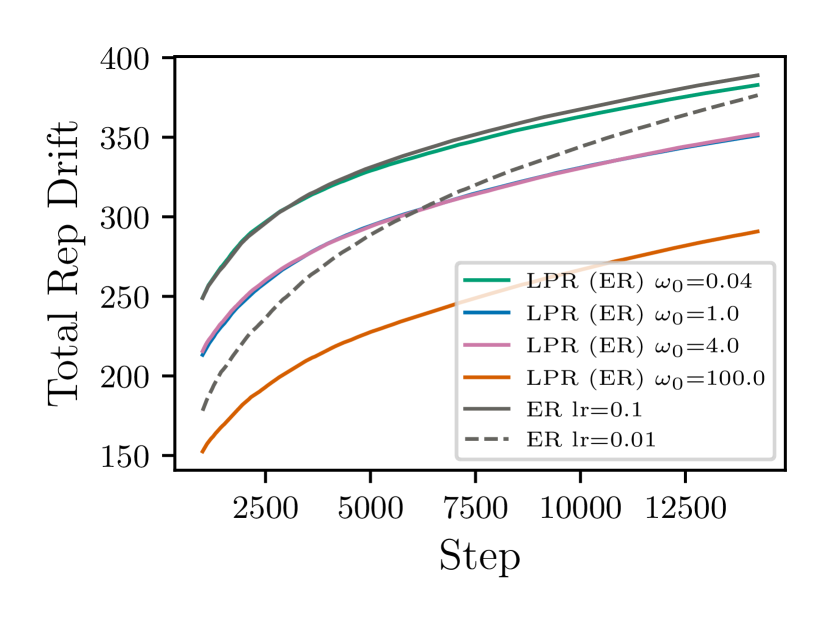
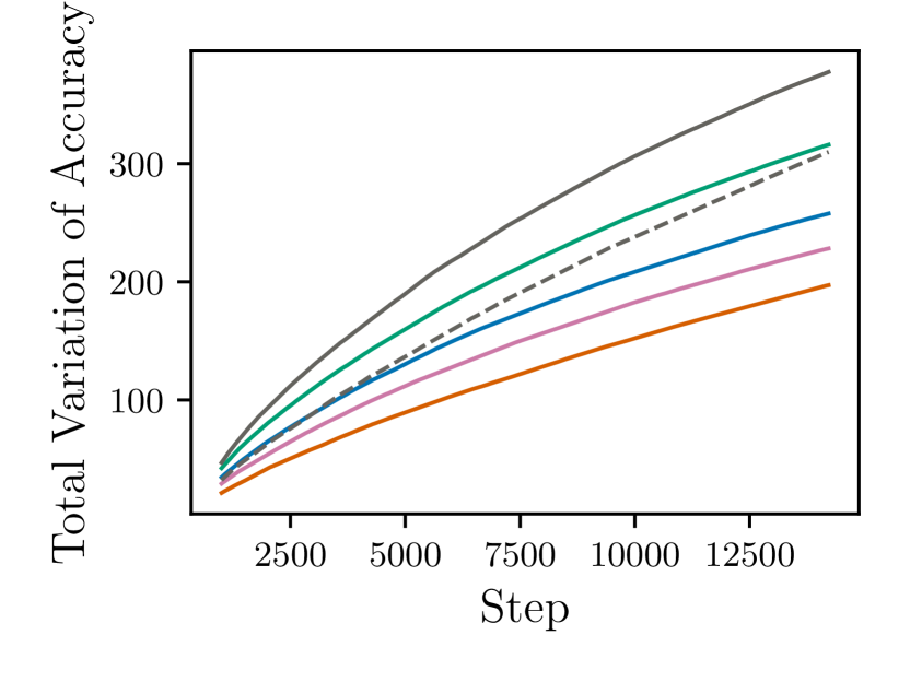
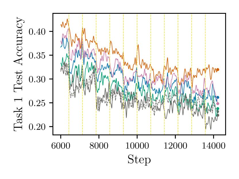
Figure 1: Internal representation and accuracy metrics vs entire training iterations for Split-CIFAR100’s task 1 test data. All LPR (ER) runs employ a learning rate of 0.1. We mark task boundaries in the right sub-figure using vertical lines. Left: dynamics of internal representation changes of task 1 data over the course of training. Middle: total variation of task 1 test accuracy. Right: task 1 test accuracy. We observe that LPR obtains lower representation drift and lower total variation of accuracy which demonstrate that LPR better preserves predictive stability of past data. This property is correlated to the overall higher accuracy as shown in the rightmost plot.

LPR’s proximal update is designed to ensure that internal representations of past data do not undergo abrupt changes. To quantify this, we consider a set $\mathcal{D}$ of test datapoints that correspond to the first CIFAR10 task (i.e. data encountered early in training). For each test datapoint $i$, we consider its internal representation $Z_{i}$ as a function of time $j$ (i.e. $Z_{i}(j)$), and we measure the stability of these representations using the following metric:

$$\text{Representation Drift}_{t}={\textstyle\sum_{j=1}^{t-1}\|Z_{i}(j+1)-Z_{i}(j)\|_{2}},$$

which captures the degree to which each gradient update changes internal representations. Figure 1 (left) demonstrates that networks trained with LPR indeed incur lower average representation drift, suggesting more stable past-data representations throughout training. Importantly, this slower representational change of LPR cannot be replicated by simply lowering the learning rate for standard gradient descent (dotted line). Finally, we note that the amount of representation drift is inversely proportional to the $\omega_{0}$ hyperparameter (see Equation 8), which is expected since LPR converges to standard gradient updates as $\omega_{0}\to 0$.

We find that representational stability is correlated with more stable predictions and overall higher accuracy. To quantify predictive stability, we consider accuracy on $\mathcal{D}$ as a function of time $j$ (i.e. $\mathrm{Acc}_{\mathcal{D}}(j)$) and report the total variation of the accuracy over training:

$$\mathrm{TV}_{t}={\textstyle\sum_{j=1}^{t-1}|\mathrm{Acc}_{\mathcal{D}}(j+1)-\mathrm{Acc}_{\mathcal{D}}(j)|},$$

which captures the degree to which each gradient update changes predictive performance on past data. In Figure 1 (middle), we observe similar trends to representation drift: LPR models yield lower total variation of accuracy, with large $\omega_{0}$ values corresponding to the least variation.

Crucially, this predictive stability leads to a higher intermediate and final accuracy on the same set of data. These results imply that the model performs better on sets of data on which it undergoes less “learning” and “forgetting.” We however highlight that Figure 1 (right) details task 1 test accuracy, not accuracy over all data. In practice, we find that the optimal $\omega_{0}$ value is dataset dependent, but generally in the range of $0.25$ to $4$ (refer to Appendix E).

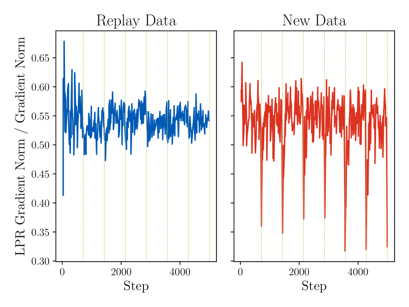
Figure 2: Ratios between post-preconditioning gradient norms and original gradient norms associated with current and replay data loss vs training iterations for LPR augmented experience replay. The vertical lines denote task boundaries.

The effect of LPR preconditioning on gradients.

Recall from Equation 8 that LPR modifies the standard gradient update with a preconditioner $P_{\ell}$. Since this preconditioner is a contraction (i.e. $\|P_{\ell}^{-1}\|<1$) the LPR parameter updates will always be smaller in magnitude than standard gradient descent updates. In Figure 2, we plot the magnitude ratio between LPR’s preconditioned gradients versus standard gradients: $\|P^{-1}\nabla\mathcal{L}(\theta)\|_{2}/\|\nabla\mathcal{L}(\theta)\|_{2}$. We split the gradient contributions of replay data versus new streaming data into the left and right plots respectively. First, we observe the magnitude ratio generally hovers around $0.55$ for both new and replay data. This result suggests that LPR may have an “effective learning rate” that is half of standard gradient descent, though we suspect that this difference alone does not account for the performance difference. More strikingly, the relative magnitude of LPR gradients shrinks dramatically whenever the data stream switches to a new task (represented by dotted lines). For new data, the “effective learning rate” decreases to $1/3$ while remaining relatively constant for replay data. Taken together, these results imply that LPR decreases parameter update magnitude by restricting parameter movement in certain directions whenever gradient updates may yield sudden changes to internal representations and past-data predictions.

5 Discussion

In this paper we present Layerwise Proximal Replay (LPR), an online continual learning method that combines experience replay with a proximal point method. We empirically demonstrate that LPR’s optimization geometry has non-trivial consequences on the predictive performance of many replay-based online continual learning methods. Importantly, the use of replay buffers and proximal optimizers complement one another. Proximal methods perform very poorly without replay (see Appendix G), and yet experience replay methods with SGD consistently under-perform their Layerwise Proximal Replay counterparts.

As discussed in Section 3, the proximal update proposed in this paper is closely related to projection methods that restrict parameter updates to a subspace orthogonal to past data activations (Zeng et al., 2019; Saha et al., 2021b; Deng et al., 2021; Lin et al., 2022; Shu et al., 2022; Zhao et al., 2023; Saha & Roy, 2023). In practice, most of these methods do not apply a “true” projection to the gradients, but rather apply “approximate projections” that often have functional forms similar to Equation 10 (see Section C.1). We believe that proximal updates, which encompass these projection approximations, provide a more natural and general space to derive new continual learning methods.

There are several possible avenues for future work. One of them is making Layerwise Proximal Replay more computationally efficient by updating the preconditioners in an online fashion, rather than recomputing them from scratch. Another is extending its proximal formulation to support correlated errors between layer activations, something that is done by Duncker et al. (2020); Kao et al. (2021) for offline continual learning without experience replay. Lastly, extending Layerwise Proximal Replay to other domains such as online reinforcement learning would be of interest.

Impact

This paper is a step toward effective continual learning of neural networks, which may cause societally impactful deep learning models such as ChatGPT to continuously integrate new data instead of being stuck in the past. Enabling these impactful models to stay up-to-date on the most recent and relevant information can affect how people interact with these models.

Appendix A Layerwise Proximal Replay Derivation

Recall the proximal update from Equation 6,

$$\theta_{j+1}=\operatorname*{arg\,min}_{\theta}\left(\left\langle\nabla\mathcal{L}(\theta_{j}),\theta-\theta_{j}\right\rangle+\frac{1}{2\eta}\|\theta-\theta_{j}\|^{2}_{2}+\sum_{\ell=1}^{L}\lambda^{(\ell)}\|Z^{(\ell)}_{j}\Theta^{(\ell)}_{j+1}-Z^{(\ell)}_{j}\Theta^{(\ell)}_{j}\|_{F}^{2}\right).$$ (11)

where $\Theta^{(i)}\in\mathbb{R}^{d^{\ell}\times d^{\ell+1}}$ is the matrix of parameters at layer $\ell$ such that $\theta=\begin{bmatrix}\mathrm{vec}(\Theta^{(1)})&\ldots&\mathrm{vec}(\Theta^{(L)})\end{bmatrix}$, $\lambda^{(\ell)}$ is the $\ell$-th layer’s Lagrange multiplier, and $Z^{(\ell)}_{j}\in\mathbb{R}^{|\mathcal{M}|\times d^{(\ell)}}$ is the hidden activations for layer $\ell$ at time $j$.

Equation 6 is equivalent to

$$\theta_{j+1} =\operatorname*{arg\,min}_{\theta}\left(\sum_{\ell=1}^{L}\left\langle\nabla\mathcal{L}(\Theta_{j}^{(\ell)}),\Theta^{(\ell)}-\Theta_{j}^{(\ell)}\right\rangle+\frac{1}{2\eta}\|\Theta^{(\ell)}-\Theta^{(\ell)}_{j}\|^{2}_{F}+\lambda^{(\ell)}\|Z^{(\ell)}_{j}\Theta^{(\ell)}_{j+1}-Z^{(\ell)}_{j}\Theta^{(\ell)}_{j}\|_{F}^{2}\right),$$ (12)

which entails that the minimization problem w.r.t. $\theta$ can be solved in a layer-wise fashion as follows.

$$\Theta^{(\ell)}_{j+1} =\operatorname*{arg\,min}_{\Theta^{(\ell)}}\left(\left\langle\nabla\mathcal{L}(\Theta_{j}^{(\ell)}),\Theta^{(\ell)}-\Theta_{j}^{(\ell)}\right\rangle+\frac{1}{2\eta}\|\Theta^{(\ell)}-\Theta^{(\ell)}_{j}\|^{2}_{F}+\frac{\omega^{\ell}}{2\eta}\|Z^{(\ell)}_{j}\Theta^{(\ell)}_{j+1}-Z^{(\ell)}_{j}\Theta^{(\ell)}_{j}\|_{F}^{2}\right)$$ (13)

where $\omega^{\ell}=2\eta\lambda^{(\ell)}$. Using the definition of the Frobenius norm, we have

$$\Theta^{(\ell)}_{j+1} =\operatorname*{arg\,min}_{\Theta^{(\ell)}}\bigg{(}\left\langle\nabla\mathcal{L}(\Theta_{j}^{(\ell)}),\Theta^{(\ell)}-\Theta_{j}^{(\ell)}\right\rangle+\frac{1}{2\eta}\mathrm{tr}\big{(}{(\Theta^{(\ell)}-\Theta^{(\ell)}_{j})}^{\mkern-6.0mu\top}(\Theta^{(\ell)}-\Theta^{(\ell)}_{j})\big{)}$$ (14)

$$\qquad\qquad\qquad+\frac{\omega^{\ell}}{2\eta}\mathrm{tr}\big{(}{(Z^{(\ell)}_{j}\Theta^{(\ell)}_{j+1}-Z^{(\ell)}_{j}\Theta^{(\ell)}_{j})}^{\mkern-6.0mu\top}(Z^{(\ell)}_{j}\Theta^{(\ell)}_{j+1}-Z^{(\ell)}_{j}\Theta^{(\ell)}_{j})\big{)}\bigg{)}$$

$$=\operatorname*{arg\,min}_{\Theta^{(\ell)}}\bigg{(}\left\langle\nabla\mathcal{L}(\Theta_{j}^{(\ell)}),\Theta^{(\ell)}-\Theta_{j}^{(\ell)}\right\rangle+\frac{1}{2\eta}\mathrm{tr}\big{(}{(\Theta^{(\ell)}-\Theta^{(\ell)}_{j})}^{\mkern-6.0mu\top}(I+\omega^{\ell}{Z_{j}^{(\ell)}}^{\mkern-6.0mu\top}Z_{j}^{(\ell)})(\Theta^{(\ell)}-\Theta^{(\ell)}_{j})\big{)}\bigg{)}$$ (15)

$$=\operatorname*{arg\,min}_{\Theta^{(\ell)}}\bigg{(}\left\langle\nabla\mathcal{L}(\Theta_{j}^{(\ell)}),\Theta^{(\ell)}-\Theta_{j}^{(\ell)}\right\rangle+\frac{1}{2\eta}\|\Theta^{(\ell)}-\Theta^{(\ell)}_{j}\|^{2}_{P_{\ell}}\bigg{)},\qquad P_{\ell}:=I+\omega^{\ell}Z^{(\ell)^{\top}}_{j}Z^{(\ell)}_{j}.$$ (16)

Setting the derivative of the term inside $\operatorname*{arg\,min}$ to $0$, we have

$$0=\nabla\mathcal{L}(\Theta_{j}^{(\ell)})+\frac{1}{\eta}(\omega^{\ell}{Z^{(\ell)}_{j}}^{\mkern-6.0mu\top}Z^{(\ell)}_{j}+I)(\Theta^{(\ell)}-\Theta^{(\ell)}_{j})$$ (17)

$$\Theta^{(\ell)}=\Theta_{j}^{(\ell)}-\eta(\omega^{\ell}{Z^{(\ell)}_{j}}^{\mkern-6.0mu\top}Z^{(\ell)}_{j}+I)^{-1}\nabla\mathcal{L}(\Theta_{j}^{(\ell)}),$$ (18)

which concludes the proof.

Appendix B The Incompatibility of Replay Data and Gradient Projections

In Section 3, we argue that gradient projection methods are largely incompatible with replay methods when additional learning on the replay buffer is desired, as is the case in online continual learning. To see why this, consider the orthogonal projection matrix $(I-\Phi^{(\ell)}(\Phi^{(\ell)^{\top}}\Phi^{(\ell)})^{-1}\Phi^{(\ell)^{\top}})$, where the matrix $\Phi^{(\ell)}\in\mathbb{R}^{d^{(\ell)}\times k}$ defines the $k$-dimensional nullspace of the projection. For most gradient projection methods, $\Phi^{(\ell)}$ is some compressed representation of past replay activations.

Let $Z^{(\ell)}=\begin{bmatrix}z_{1}^{(\ell)\top};\ldots;z_{m}^{(\ell)\top}\end{bmatrix}\in\mathbb{R}^{m\times d^{(\ell)}}$ be the activations of $m$ replay datapoints used to compute the replay loss. We can decompose these activations as

$$Z^{(\ell)\top}=\Phi^{(\ell)}A+R,$$

where $A\in\mathbb{R}^{k\times m}$ and $R$ is some matrix orthogonal to $\Phi^{(\ell)}$. If $\Phi^{(\ell)}$ is a good approximation of all replay activations, then we expect $\|R\|_{F}$ to be small.

When computing the replay loss, note that $Z^{(\ell)}$ interacts with the parameters $\Theta^{(\ell)}$ through the matrix multiplication $Z^{(\ell)}\Theta^{(\ell)}$. Therefore, applying standard vector-Jacobian product backpropagation rules, the replay loss gradient is given as

$$\nabla_{\Theta}^{(\ell)}\mathcal{L}_{\mathrm{replay}}=Z^{(\ell)\top}V=\left(\Phi^{(\ell)}A+R\right)V$$

for some matrix $V\in\mathbb{R}^{m\times d^{(\ell+1)}}$ The projected gradient is thus equal to:

$$\left(I-\Phi^{(\ell)}(\Phi^{(\ell)^{\top}}\Phi^{(\ell)})^{-1}\Phi^{(\ell)^{\top}}\right)\nabla_{\Theta}^{(\ell)}\mathcal{L}_{\mathrm{replay}}=\left(I-\Phi^{(\ell)}(\Phi^{(\ell)^{\top}}\Phi^{(\ell)})^{-1}\Phi^{(\ell)^{\top}}\right)\left(\Phi^{(\ell)}A+R\right)V=RV.$$

If $\|R\|_{F}\approx 0$ (which again will be the case if $\Phi^{(\ell)}$ is a good approximation of all replay activations), then almost all of the replay gradient will be projected out.

Appendix C Extended Related Work

There are two papers that employ orthogonal gradient projection for online continual learning: A-GEM (Chaudhry et al., 2018) and AOP (Guo et al., 2022). Neither of them employs experience replay. AOP is perhaps the closest method to LPR since it employs an incremental algorithm to approximate the layerwise preconditioner $P^{\ell}=({Z^{\ell}}^{\mkern-6.0mu\top}Z^{\ell}+\alpha I)^{-1}$ with a very low $\alpha$, whose form is identical to LPR’s layerwise preconditioner up to a constant factor. However, there are crucial methodological and empirical differences between LPR and AOP. AOP does not use experience replay and their $Z^{\ell}$ consists of a mini-batch’s average activations. In addition, because past data activations in $Z^{\ell}$ are never updated to the updated model’s feed-forward activations of the same data, AOP’s $Z^{\ell}$ becomes stale over time. Last but not least, AOP severely underperforms compared to replay methods in all of our evaluations.

Our work is also related to prior work that highlights the importance of how neural networks are optimized during continual learning with or without memory constraints (Ash & Adams, 2020; Kao et al., 2021; De Lange et al., 2022; Konishi et al., 2023). Kao et al. (2021) combines online Laplace approximation and the K-FAC (Martens & Grosse, 2015) preconditioner to tackle offline continual learning. A concurrent work from Hess et al. (2023) also proposed the use of orthogonal gradient projection methods with experience replay motivated by the stability gap phenomenon (De Lange et al., 2022) for both offline and online continual learning. However, they do so without experimental results as of now.

C.1 The Proximal Perspective of OWM and GPM Parameter Updates

Consider the proximal update

$$\Theta^{(\ell)}_{j+1} =\operatorname*{arg\,min}_{\Theta^{(\ell)}}\left(\left\langle\nabla\mathcal{L}(\Theta_{j}^{(\ell)}),\Theta^{(\ell)}-\Theta_{j}^{(\ell)}\right\rangle+\frac{1}{2\eta}\|\Theta^{(\ell)}-\Theta^{(\ell)}_{j}\|^{2}_{2}+\frac{1}{2\eta}\sum_{m\in M^{\ell}}\omega_{m}\|m\Theta^{(\ell)}-m\Theta^{(\ell)}_{j}\|_{2}^{2}\right).$$ (19)

where $\Theta_{j}^{(\ell)}\in\mathbb{R}^{d^{\ell}\times d^{\ell+1}}$ is the layer $l$ weight matrix at optimization step $j$, $\nabla\mathcal{L}(\Theta_{j}^{(\ell)})$ is the objective gradient, $M^{\ell}\in\mathbb{R}^{n^{\ell}\times d^{\ell}}$ is the size $n^{\ell}$ “representative set” of $\ell$-th layer’s past activations $m\in\mathbb{R}^{1\times d^{\ell}}$, $\omega_{m}\in\mathbb{R}_{\geq 0}$ is $m$’s importance weight, and $\eta$ is the learning rate. The representative set $M^{\ell}$ is allowed to contain pseudo-activation that may not have been observed before. We note Equation 19 is a “weighted version” of the LPR proximal update where error on different entries $Z^{(l)}$ are penalized to different degrees, dependent on $\omega_{m}$.

This proximal update, with appropriate choices of $M^{\ell}$, $\omega_{m}$, and $\mathcal{L}(\Theta_{j}^{(\ell)})$, recovers OWM-based methods’ projected gradient update (Zeng et al., 2019; Guo et al., 2022)

$$\Theta^{(\ell)}_{j+1}=\Theta_{j}^{(\ell)}-\eta(I-{M^{\ell}}^{\mkern-6.0mu\top}(\alpha I+M^{\ell}{M^{\ell}}^{\mkern-6.0mu\top})^{-1}M^{\ell})\nabla\mathcal{L}(\Theta_{j}^{(\ell)})$$ (20)

where $\alpha>0$, and GPM-based methods’ scaled projected gradient update (Saha et al., 2021b; Deng et al., 2021; Shu et al., 2022; Saha & Roy, 2023)

$$\Theta^{(\ell)}_{j+1}=\Theta_{j}^{(\ell)}-\eta(I-{M^{\ell}}^{\mkern-6.0mu\top}\Lambda^{\ell}M^{\ell})\nabla\mathcal{L}(\Theta_{j}^{(\ell)})$$ (21)

where $\Lambda^{\ell}\in\mathbb{R}^{k\times k}$ is a diagonal matrix whose entries are in $(0,1]$ and $k<d^{l-1}$.

Proof.

The derivative of the proximal objective in Equation 19 is

$$\nabla\mathcal{L}(\Theta_{j}^{(\ell)})+\frac{1}{\eta}\left(I+\sum_{m\in M^{\ell}}\omega_{m}m^{\top}m\right)(\Theta^{(\ell)}-\Theta_{j}^{(\ell)}).$$ (22)

Setting this to $0$ and rearranging the terms, we have

$$\Theta^{(\ell)} =\Theta_{j}^{(\ell)}-\eta\left(I+\sum_{m\in M^{\ell}}\omega_{m}m^{\top}m\right)^{-1}\nabla\mathcal{L}(\Theta_{j}^{(\ell)})$$ (23)

$$=\Theta_{j}^{(\ell)}-\eta\left(I+{M^{\ell}}^{\mkern-6.0mu\top}\Omega M^{\ell}\right)^{-1}\nabla\mathcal{L}(\Theta_{j}^{(\ell)})$$ (24)

where $\Omega\in\mathbb{R}^{k\times k}$ is a diagonal matrix with $\omega_{k}$ on its diagonal. Using Woodbury matrix identity, we then have

$$\Theta^{(\ell)}=\Theta_{j}^{(\ell)}-\eta\left(I-{M^{\ell}}^{\mkern-6.0mu\top}\Lambda^{\ell}M^{\ell}\right)^{-1}\nabla\mathcal{L}(\Theta_{j}^{(\ell)})$$ (25)

$$\Lambda^{\ell}\coloneqq(\Omega^{-1}+M^{\ell}{M^{\ell}}^{\mkern-6.0mu\top})^{-1}.$$ (26)

If we set the rows of $M^{\ell}$ to the average embedding of mini-batch for all past mini-batches (each embedding computed right after training on that mini-batch), set $\Omega^{-1}=\alpha I$, and set $\mathcal{L}(\Theta_{j}^{(\ell)})$ to the current data batch loss (without replay loss) in Equation 26, and we recover OWM’s projected gradient update.

If we set the rows of $M^{\ell}$ to core gradient space’s (Saha et al., 2021a) orthonormal basis vectors, set diagonal elements of $\Omega^{-1}$ to the soft projection scores between $0$ and $\infty$ associated with each basis vectors, and set $\nabla\mathcal{L}(\Theta_{j}^{(\ell)})$ to GPM method specific loss in Equation 26, we recover GPM’s projected gradient update since the diagonal entries of $\Lambda^{\ell}=(\Omega^{-1}+M^{\ell}{M^{\ell}}^{\mkern-6.0mu\top})^{-1}$ becomes $\lambda_{i}=\frac{\omega_{i}}{\omega_{i}+1}$. The basis vector importance weight $\omega_{i}$ can individually be set between $0$ and $\infty$ to cause $\lambda_{i}$ to be between $[0,1]$. ∎

Appendix D Parameterizing Layerwise Importance Weights

We propose a simple method for setting the proximal penalty strength hyperparameters $\omega_{0}^{\ell}$ for every layer using two scalar hyperparameters $\omega_{0},\beta$. The scalar $\omega_{0}\geq 0$ represents the base proximal penalty strength for all network layers. The scalar $\beta\geq 0$ controls the magnitude of a per-layer scaling term $c^{\ell}$ that is applied to $\omega_{0}$ based on how many “effective activation vectors” can be constructed from a single replay buffer exemplar for matrix multiplication for that layer. We denote this per-layer effective activation vector count by $n_{eff}^{\ell}$ and note that $n_{eff}^{\ell}$ is predetermined for each layer.

Concretely, the formula for $\omega_{0}^{\ell}$ is

$$\omega_{0}^{\ell}=\frac{\omega_{0}}{c^{\ell}},\quad\quad\quad c^{\ell}=(n_{eff}^{\ell})^{\beta}.$$ (27)

We give specific examples of $n_{eff}^{\ell}$ for linear, 2D convolution, and 2D batch normalization layers, all of which are used in ResNet18. For ResNet18’s linear layer of depth $l$, a single replay buffer exemplar translates to a single input embedding of size $d^{l-1}$. Therefore, $n_{eff}^{\ell}$ is simply $1$. For ResNet18’s 2D convolution layer of depth $l$, a single replay buffer exemplar translates to an input feature map of size $C_{\text{in}}\times W_{\text{f}}\times H_{\text{f}}$, where $C_{\text{in}}$ refers to the input channel dimension, $W_{\text{f}}$ and $H_{\text{f}}$ represents the feature map’s width and height. To convert 2D convolution on this feature map to matrix multiplication, the input feature map must be converted to a matrix shape $N_{\text{P}}\times(C_{\text{in}}*W_{\text{k}}*H_{\text{k}})$ where $N_{\text{P}}$ denotes the number of patches from the input feature map to be matrix multiplied with the convolution weights, $W_{\text{k}}$ and $H_{\text{k}})$ denotes convolution kernel’s width and height. Therefore, $n_{eff}^{\ell}$ is equal to $N_{\text{P}}$ specific to the $l$-th layer’s convolution operation. Lastly, for ResNet18’s 2D batch normalization layer of depth $l$, a single replay buffer exemplar again translates to an input feature map of size $C_{\text{in}}\times W_{\text{f}}\times H_{\text{f}}$. Since 2D batch normalization applies a channel-wise normalization and scaling, it can be seen as $C_{\text{in}}$ independent 1D linear map. For each 1D linear map, the corresponding channel’s feature map is independently converted to a vector of size $(W_{\text{f}}*H_{\text{f}})$. Therefore, $n_{eff}^{\ell}$ is equal to $(W_{\text{f}}*H_{\text{f}})$ for 2D batch normalization.

Appendix E Additional Experiment Details

We discuss the datasets we evaluate on in more detail. Split-CIFAR100 dataset is based on (Krizhevsky et al., 2009), which contains 50,000 training images of size 32x32 that belong to 100 classes. Split-TinyImageNet dataset is based on (Le & Yang, 2015), which contains 100,000 training images of size 64x64 that belong to 200 classes. The CLEAR dataset (Lin et al., 2021) contains 33,000 training images of size 224 x 224 that belong to 11 classes. CLEAR is designed to have a smooth temporal evolution of visual concepts with real-world imagery, which is a scenario more likely to be encountered in real life than the commonly used Permuted MNIST based off (LeCun et al., 1998) or the Core50 domain-incremental learning benchmark (Lomonaco & Maltoni, 2017).

Hyperparameters for all baselines and LPR augmented baseline runs from the paper were selected once per dataset, based on medium memory size online continual learning experiments (memory size 2000 for Split CIFAR100, 4000 for Split TinyImageNet, and 2000 for Online CLEAR). For each baseline method, we searched across method-specific hyperparameters and selected the configuration that yielded the best final average validation accuracy on a single seed. For LPR augmented baseline methods, we searched across LPR hyperparameters $\omega_{0},\beta$ on top of the selected baseline configuration per method in a likewise fashion.

For all baseline methods on all datasets, we searched across their learning rates between $\{0.01,0.05,0.1\}$. For DER, we additionally searched across the replay loss weight between $\{0.1,0.5,1.\}$ and the logit matching loss weight between $\{0.1,0.5,1.\}$. For EMA, we additionally searched across the exponential moving average momentum between $\{0.99,0.995,0.999\}$. For LODE, we searched across the old/new class distinction loss weighting $\rho$ between $\{0.,0.05,0.1\}$. We note that setting $\rho=0.$ recovers ER-ACE (Caccia et al., 2021).

For all LPR runs on all datasets, we searched across $\omega_{0}$ between $\{0.04,0.25,1.,4.,100.\}$ and $\beta$ between $\{1.,2.\}$ on top of the selected baseline configurations. The preconditioner update interval was set to $T=10$ for all experiments, meaning that we updated the preconditioners once every $10$ new data batches.

Tables 5, 6 and 7 contains the selected hyperparameters for replay baselines and its LPR augmentations. In addition to these hyperparameters, we also present replay baseline-specific hyperparameters. DER’s replay loss and logit matching loss weights were $1$ and $1$ for Split-CIFAR100, $1$ and $0.5$ for Split-TinyImageNet, and $0.5$ and $1$ for Online CLEAR. EMA’s momentum was set to $0.999$ for all datasets. LODE’s $\rho$ was set to $0.1$ for Split-CIFAR100 and Split-TinyImageNet.

Method	Split-CIFAR100	Split-TinyImageNet	Online CLEAR
ER	0.1	0.01	0.01
DER	0.05	0.01	0.1
EMA	0.05	0.01	0.05
LODE	0.1	0.01	-

Table 5: Selected learning rates for experience replay baselines.

Method	Split-CIFAR100	Split-TinyImageNet	Online CLEAR
LPR (ER)	4	0.25	1
LPR (DER)	1	0.25	0.25
LPR (EMA)	0.04	0.25	0.25
LPR (LODE)	1	0.25	-

Table 6: Selected $\omega_{0}$ for LPR augmented experience replay baselines.

Method	Split-CIFAR100	Split-TinyImageNet	Online CLEAR
LPR (ER)	2	2	1
LPR (DER)	1	2	1
LPR (EMA)	1	2	1
LPR (LODE)	2	2	-

Table 7: Selected $\beta$ for LPR augmented experience replay baselines.

Appendix F Computation

We report the computation comparison between ER and LPR runs on all datasets on memory constrained experiments.

We report computation time on replay buffer size $1000$ experiments. ER took 7 minutes, 35 minutes, and 2 hours 10 minutes to run on Split-CIFAR100, Split-TinyImageNet, and Online CLEAR datasets respectively. LPR took 20 minutes, 2 hours 30 minutes, and 5 hours 45 minutes to run respectively.

We report computation time on replay buffer size $2000$ experiments. ER took 7 minutes, 39 minutes, and 2 hours 15 minutes to run on Split-CIFAR100, Split-TinyImageNet, and Online CLEAR datasets respectively. LPR took 28 minutes, 3 hours 4 minutes, and 7 hours 11 minutes to run respectively.

Appendix G Gradient Projection Results on Online Continual Learning

Split-CIFAR100
Method	Acc	AAA	WC-Acc
AOP	0.0472 ± 0.0010	0.1293 ± 0.0029	0.0411 ± 0.0022
AGEM	0.0327 ± 0.0024	0.1004 ± 0.0027	0.0317 ± 0.0023
LPR (ER)	0.4244 ± 0.0051	0.4644 ± 0.0040	0.2260 ± 0.0057
Split-TinyImageNet
Method	Acc	AAA	WC-Acc
AOP	0.0363 ± 0.0017	0.0929 ± 0.0018	0.0298 ± 0.0015
AGEM	0.0295 ± 0.002	0.0683 ± 0.0033	0.025± 0.0012
LPR (ER)	0.3686 ± 0.0055	0.4153 ± 0.0075	0.2437 ± 0.0025
Online CLEAR
Method	Acc	AAA	WC-Acc
AOP	0.5323 ± 0.0056	0.5596 ± 0.0055	0.5050 ± 0.0036
AGEM	0.5731 ± 0.0050	0.5272 ± 0.0025	0.4748 ± 0.0015
LPR (ER)	0.7411 ± 0.0040	0.7120 ± 0.0031	0.6834 ± 0.0040

Table 8: Online continual learning results with mean and standard error computed across 5 random seeds.

Method	Split-CIFAR100	Split-TinyImageNet	Online CLEAR
AGEM	0.05	0.10	0.01
AOP	0.05	0.01	0.05

Table 9: Optimal learning rates for gradient projection baselines, AGEM and AOP.

We evaluate two gradient projection-based methods, AGEM (Chaudhry et al., 2018) and AOP (Guo et al., 2022), on the online versions of the Split-CIFAR100, Split-TinyImageNet, and CLEAR datasets and compare them to our proposed LPR method. The same network architecture is utilized for AGEM and AOP as for LPR, with the optimal learning rate, selected through our hyper-parameter search, reported in Table 9. We report the evaluation results over 5 seeds in Table 8. We observe a huge performance gap between the two projection methods and our LPR method on online class-incremental learning, which we attribute to the fact that the gradient projection methods underfit the data stream. For online domain-incremental learning, LPR still obtains a big performance gain compared to AGEM and AOP.

References

- Ash & Adams (2020) Ash, J. and Adams, R. P. On warm-starting neural network training. Advances in neural information processing systems, 33:3884–3894, 2020.
- Asi & Duchi (2019) Asi, H. and Duchi, J. C. Stochastic (approximate) proximal point methods: Convergence, optimality, and adaptivity. SIAM Journal on Optimization, 29(3):2257–2290, January 2019. ISSN 1095-7189. doi: 10.1137/18m1230323. URL http://dx.doi.org/10.1137/18M1230323.
- Buzzega et al. (2020) Buzzega, P., Boschini, M., Porrello, A., Abati, D., and Calderara, S. Dark experience for general continual learning: a strong, simple baseline. Advances in neural information processing systems, 33:15920–15930, 2020.
- Caccia et al. (2021) Caccia, L., Aljundi, R., Asadi, N., Tuytelaars, T., Pineau, J., and Belilovsky, E. New insights on reducing abrupt representation change in online continual learning. arXiv preprint arXiv:2104.05025, 2021.
- Caccia et al. (2020) Caccia, M., Rodriguez, P., Ostapenko, O., Normandin, F., Lin, M., Caccia, L., Laradji, I., Rish, I., Lacoste, A., Vazquez, D., et al. Online fast adaptation and knowledge accumulation: a new approach to continual learning. arXiv preprint arXiv:2003.05856, 2020.
- Carta et al. (2023a) Carta, A., Pellegrini, L., Cossu, A., Hemati, H., and Lomonaco, V. Avalanche: A pytorch library for deep continual learning. Journal of Machine Learning Research, 24(363):1–6, 2023a.
- Carta et al. (2023b) Carta, A., Van de Weijer, J., et al. Improving online continual learning performance and stability with temporal ensembles. arXiv preprint arXiv:2306.16817, 2023b.
- Chaudhry et al. (2018) Chaudhry, A., Ranzato, M., Rohrbach, M., and Elhoseiny, M. Efficient lifelong learning with a-gem. arXiv preprint arXiv:1812.00420, 2018.
- Chaudhry et al. (2019) Chaudhry, A., Rohrbach, M., Elhoseiny, M., Ajanthan, T., Dokania, P., Torr, P., and Ranzato, M. Continual learning with tiny episodic memories. In Workshop on Multi-Task and Lifelong Reinforcement Learning, 2019.
- De Lange et al. (2022) De Lange, M., van de Ven, G., and Tuytelaars, T. Continual evaluation for lifelong learning: Identifying the stability gap. arXiv preprint arXiv:2205.13452, 2022.
- Deng et al. (2021) Deng, D., Chen, G., Hao, J., Wang, Q., and Heng, P.-A. Flattening sharpness for dynamic gradient projection memory benefits continual learning. Advances in Neural Information Processing Systems, 34:18710–18721, 2021.
- Drusvyatskiy (2017) Drusvyatskiy, D. The proximal point method revisited, 2017.
- Duncker et al. (2020) Duncker, L., Driscoll, L., Shenoy, K. V., Sahani, M., and Sussillo, D. Organizing recurrent network dynamics by task-computation to enable continual learning. Advances in neural information processing systems, 33:14387–14397, 2020.
- Farajtabar et al. (2020) Farajtabar, M., Azizan, N., Mott, A., and Li, A. Orthogonal gradient descent for continual learning. In International Conference on Artificial Intelligence and Statistics, pp. 3762–3773. PMLR, 2020.
- French (1999) French, R. M. Catastrophic forgetting in connectionist networks. Trends in cognitive sciences, 3(4):128–135, 1999.
- Guo et al. (2022) Guo, Y., Hu, W., Zhao, D., and Liu, B. Adaptive orthogonal projection for batch and online continual learning. In Proceedings of the AAAI Conference on Artificial Intelligence, volume 36, pp. 6783–6791, 2022.
- Hess et al. (2023) Hess, T., Tuytelaars, T., and van de Ven, G. M. Two complementary perspectives to continual learning: Ask not only what to optimize, but also how. arXiv preprint arXiv:2311.04898, 2023.
- Kao et al. (2021) Kao, T.-C., Jensen, K., van de Ven, G., Bernacchia, A., and Hennequin, G. Natural continual learning: success is a journey, not (just) a destination. Advances in neural information processing systems, 34:28067–28079, 2021.
- Konishi et al. (2023) Konishi, T., Kurokawa, M., Ono, C., Ke, Z., Kim, G., and Liu, B. Parameter-level soft-masking for continual learning. arXiv preprint arXiv:2306.14775, 2023.
- Krizhevsky et al. (2009) Krizhevsky, A., Hinton, G., et al. Learning multiple layers of features from tiny images, 2009.
- Le & Yang (2015) Le, Y. and Yang, X. Tiny imagenet visual recognition challenge. CS 231N, 7(7):3, 2015.
- LeCun et al. (1998) LeCun, Y., Bottou, L., Bengio, Y., and Haffner, P. Gradient-based learning applied to document recognition. Proceedings of the IEEE, 86(11):2278–2324, 1998.
- Liang & Li (2023) Liang, Y.-S. and Li, W.-J. Loss decoupling for task-agnostic continual learning. In Thirty-seventh Conference on Neural Information Processing Systems, 2023.
- Lin et al. (2022) Lin, S., Yang, L., Fan, D., and Zhang, J. Trgp: Trust region gradient projection for continual learning. arXiv preprint arXiv:2202.02931, 2022.
- Lin et al. (2021) Lin, Z., Shi, J., Pathak, D., and Ramanan, D. The clear benchmark: Continual learning on real-world imagery. In Thirty-fifth conference on neural information processing systems datasets and benchmarks track (round 2), 2021.
- Lomonaco & Maltoni (2017) Lomonaco, V. and Maltoni, D. Core50: a new dataset and benchmark for continuous object recognition. In Conference on robot learning, pp. 17–26. PMLR, 2017.
- Martens & Grosse (2015) Martens, J. and Grosse, R. Optimizing neural networks with kronecker-factored approximate curvature. In International conference on machine learning, pp. 2408–2417. PMLR, 2015.
- Parikh & Boyd (2014) Parikh, N. and Boyd, S. Proximal algorithms. Found. Trends Optim., 1(3):127–239, jan 2014. ISSN 2167-3888. URL https://doi.org/10.1561/2400000003.
- Saha & Roy (2023) Saha, G. and Roy, K. Continual learning with scaled gradient projection. arXiv preprint arXiv:2302.01386, 2023.
- Saha et al. (2021a) Saha, G., Garg, I., Ankit, A., and Roy, K. Space: Structured compression and sharing of representational space for continual learning. IEEE Access, 9:150480–150494, 2021a.
- Saha et al. (2021b) Saha, G., Garg, I., and Roy, K. Gradient projection memory for continual learning. arXiv preprint arXiv:2103.09762, 2021b.
- Shu et al. (2022) Shu, K., Li, H., Cheng, J., Guo, Q., Leng, L., Liao, J., Hu, Y., and Liu, J. Replay-oriented gradient projection memory for continual learning in medical scenarios. In 2022 IEEE International Conference on Bioinformatics and Biomedicine (BIBM), pp. 1724–1729, 2022. doi: 10.1109/BIBM55620.2022.9995580.
- Soutif-Cormerais et al. (2023) Soutif-Cormerais, A., Carta, A., Cossu, A., Hurtado, J., Hemati, H., Lomonaco, V., and de Weijer, J. V. A comprehensive empirical evaluation on online continual learning, 2023.
- van de Ven et al. (2022) van de Ven, G. M., Tuytelaars, T., and Tolias, A. S. Three types of incremental learning, December 2022. URL http://dx.doi.org/10.1038/s42256-022-00568-3.
- Zeng et al. (2019) Zeng, G., Chen, Y., Cui, B., and Yu, S. Continual learning of context-dependent processing in neural networks. Nature Machine Intelligence, 1(8):364–372, 2019.
- Zhang et al. (2022) Zhang, Y., Pfahringer, B., Frank, E., Bifet, A., Lim, N. J. S., and Jia, Y. A simple but strong baseline for online continual learning: Repeated augmented rehearsal. Advances in Neural Information Processing Systems, 35:14771–14783, 2022.
- Zhao et al. (2023) Zhao, Z., Zhang, Z., Tan, X., Liu, J., Qu, Y., Xie, Y., and Ma, L. Rethinking gradient projection continual learning: Stability/plasticity feature space decoupling. In Proceedings of the IEEE/CVF Conference on Computer Vision and Pattern Recognition, pp. 3718–3727, 2023.