Quantum state discrimination enhanced by path signature

Abstract

Quantum state discrimination plays an essential role in quantum technology, crucial for quantum error correction, metrology, and sensing. While conventional methods rely on integrating readout signals or classifying raw signals, we developed a method to extract information about state transitions during readout, based on the path signature method, a tool for analyzing stochastic time series. The hardware experiments demonstrate an improvement in transmon qutrit state readout fidelity from $85.9\pm 1.0\%$ to $91.0\pm 0.5\%$, without the need for additional hardware. This method has the potential to become a foundational tool for quantum technology.

Rapid high-fidelity single-shot readout is essential for engineering quantum processors. The recent demonstration of quantum error correction highlights that a considerable amount of the error budget is related to the readout process, therefore enhancement in readout can benefit quantum error correction Acharya et al. (2023). Dispersive readout stands as one of the most widely-used readout mechanisms Kohler (2018); Blais et al. (2004). The resonator coupled to the qubit exhibits a frequency shift that depends on the state of the qubit, therefore, the qubit state can be inferred by probing the resonance mode. This mechanism has been demonstrated across various solid-state qubits architectures, including spin-qubits Crippa et al. (2019); D’Anjou and Burkard (2019), quantum dots Colless et al. (2013); Rossi et al. (2017); Burkard and Petta (2016), superconducting qubits Wallraff et al. (2005); Walter et al. (2017).

The conventional state discrimination method for dispersive readout integrates the readout signal and produces a single data point that reflects the resonator response at the probing frequency Krantz et al. (2019). This method assumes the qubit state remains steady during readout, which is not always the case. When the measurement pulse length is not negligible compared to the qubit relaxation time, the qubit may decay during the measurement Elder et al. (2020); Thorbeck et al. (2023). When the probing signal is driven too strongly, it may induce state transitions due to the Stark-shift effect Khezri et al. (2023); Sank et al. (2016). On the other hand, the dispersive readout signals capture a time series of resonator responses, enabling the potential for continuous tracking of the qubit state. To take this advantage, various standard statistical learning techniques have been employed to analyze the readout signal, such as Linear Discriminant Analysis (LDA), Quadratic Discriminant Analysis (QDA), and Support Vector Machines (SVMs) Magesan et al. (2015). In addition, machine learning models such as the Hidden Markov Model (HMM) Martinez et al. (2020), Feed-forward Neural Networks (FFNN) Lienhard et al. (2022), and Variational Autoencoders (VAE) Luchi et al. (2023) have been applied to improve the readout fidelity by taking the time-series data as inputs. Although they show improvements, the models are often treated as black boxes and do not emphasize their physical significance.

This study focuses on feature engineering for capturing information about during measurement state transitions. Consider a cumulative sum of the collected signal that forms a trajectory that can be modeled as a stochastic controlled differential equation. The qubit’s state and noise are random variables influencing the trajectory. Motivated by this structure, we employ the stochastic time series tool “path signature” to extract information from the readout signal Lyons (2014a); Chevyrev and Kormilitzin (2016); Fermanian et al. (2023). Our findings show that the signature feature captures information about state transition events during the readout, and by applying this advantage, its application considerably boosts readout fidelity.

Consider a resonator coupled to a qubit, where the resonator has resonance frequency $\omega_{r}=\omega_{r}^{(0)}$ when the qubit is at the ground state. It exhibits a dispersive shift $\chi_{i}$ when the qubit is in state $\ket{i}$, resulting in the resonator frequency becoming $\omega_{r}^{(i)}=\omega_{r}+\chi_{i}$. See Fig.1(a). Consider the probing signal sent to the resonator has frequency $\omega_{p}$ with a pulse envelope $f_{t}$, where $t$ denotes the time. The response signal is a complex number time series, denoted as $R_{t}$. The in-phase channel signal $I_{t}=\mathrm{Re}(R_{t})$ and the quadrature channel $Q_{t}=\mathrm{Im}(R_{t})$ are the real and imaginary part of the response signal, respectively. The conventional way of implementing state discrimination is to find the integrated signal $\tilde{R}=\int R_{t}f(t)\mathrm{d}t$, and classify $\tilde{R}$ for different states Wallraff et al. (2005); Walter et al. (2017); Heinsoo et al. (2018). See to Fig.1(b). Instead of doing simple integration of the signal, we define a two-dimensional variable $X_{t}=\{I_{t},Q_{t}\}$, and construct a trajectory $F_{t}=\int^{t}_{0}\mathrm{d}X_{t}$ which is the cumulated sum of $X_{t}$. Now consider the composition of the increment ${\rm d}X_{t}$ which corresponds to the experimentally received signal $R_{t}$. Referring to Fig.1(c), we model the signal to contain a deterministic term $F_{k}$ which is dependent on the qubit state, and a noise term as a random variable for Gaussian noise ${\rm d}\epsilon_{t}$, therefore

$${\rm d}X^{k}_{t}={\rm d}F^{k}_{t}+{\rm d}\epsilon_{t}$$ (1)

where $X^{k}_{t}$ is a random variable that denotes the received signal at time $t$, and $F^{k}_{t}$ is the resonator noiseless response at time $t$. The signal contains two channels, with $k\in\{I,Q\}$ representing the in-phase and quadrature-phase channels, respectively.

The signature of a multi-dimensional time-series path is a graded, infinite collection of iterated integrals, where the signature of a path $X$ with dimension $d$ up to degree $N$ is the collection

$$\operatorname{\mathrm{Sig}}^{N}(X):=\left(\underset{0<t_{1}<\cdots<t_{k}<1}{\int\cdots\int}\frac{\mathrm{d}X_{i_{1}}}{\mathrm{d}t}(t_{1})\cdot\frac{\mathrm{d}X_{i_{2}}}{\mathrm{d}t}(t_{2})\cdots\frac{\mathrm{d}X_{i_{k}}}{\mathrm{d}t}(t_{k})\mathrm{d}t_{1}\cdots\mathrm{d}t_{k}\right)_{\begin{subarray}{c}\!\!1\leq i_{1},\ldots,i_{k}\leq d\\ \!\!k=0,1,2,\ldots,N\end{subarray}}.$$ (2)

The signature describes the time series in a global, geometric, and interacting way. For example, the degree $1$ signatures are the displacement between the endpoint and the startpoint in different dimensions, and the degree $2$ signatures describe the area enclosed by the loop formed by building a curve from the time series of increments and closing it with the chord from the end-point to the start-point. See Lyons (2014a); Chevyrev and Kormilitzin (2016); Fermanian et al. (2023) for more information about the signature method.

Signatures of variable $F_{t}$ have physical significance. The degree 1 signature is given by $S^{(1)}(F)=\{F_{t}-F_{0}\}$. Since $F_{0}$ is always zero in practice, and $F_{t}$ is the integral of the received signal, $S^{(1)}(F)$ falls back to the traditional approach of integrating the signal. The degree 2 signature corresponds to the Lévy area $A$ of a 2D path $\{X_{i}(t),X_{j}(t)\}$, given by

$$A=\frac{1}{2}\left(S(X)^{i,j}-S(X)^{j,i}\right),$$ (3)

where $S(X)^{i,j}$ corresponds to the terms in Eq.(2) with $k=2$, $i_{1}=i,i_{2}=j$. The higher-order signatures generalize the definition of Lévy area to higher dimension volumes.

Consider a state transition that occurred at time $t_{s}$ during the measurement. For $t<t_{s}$, $\mathrm{d}F_{t}$ remains constant, resulting in a linear trajectory under the assumption of a noiseless signal and negligible ramp-up and ramp-down duration of the signal envelope. For $t>t_{s}$, $\mathrm{d}X_{t}$ is a different value and forms discontinuity of the signal, creating a new linear segment starting from the end of the previous trajectory. Referring to Fig.1(d), the shaded area, which appears only if a transition occurs, is captured by the degree 2 signatures. An exception arises when the trajectories before and after $t_{s}$ are exactly opposite in directions. To address this, we employ the time-augmentation method during the evaluation of signatures, adding time as an additional dimension to the data, which ensures the detection of state transitions.

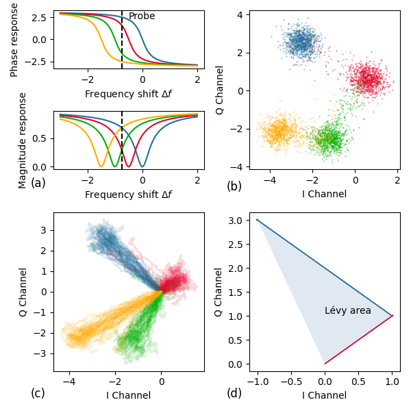
Figure 1: A simulated model for dispersive readout of a transmon coupled to a resonator. The blue, red, green, and yellow colors denote the transmon in the $\ket{0}$, $\ket{1}$, $\ket{2}$, and $\ket{3}$ states, respectively. (a) The phase (top) and amplitude (bottom) response of a resonator. (b) The simulated distribution by integrating the signal on the IQ plane. (c) The constructed trajectory is based on Eq.(1). (d) A generic example of Lévy area of the noiseless signal. The trajectory moves towards the direction where the qubit is in $\ket{1}$ initially; then it shifts direction to the $\ket{0}$ state when the qubit decays.

To benchmark the performance of the signature approach to characterize the state transition during the measurement of real hardware, we first developed a simulator to generate synthetic traces according to Eq.(1) from a dataset collected on the hardware. The detailed characterization of this device has been reported in a previous work Cao et al. (2022, 2023). For the details of the data collection, please refer to App.A. The mean values of the synthetic traces are evaluated from the average values of the experimental dataset and then Gaussian noise is added to the mean value to generate synthetic traces. The Gaussian noise’s standard deviation corresponds to the experimental dataset’s standard deviation at each time point. We defined the simulated transition time $t_{s}$ for each trace. Before $t_{s}$, traces follows the experimental traces of state $\ket{1}$, and after $t_{s}$, they follow the traces of state $\ket{0}$. We generated a synthetic dataset of 10,000 traces with a uniform distribution of $t_{s}$. This dataset was randomly divided into training and testing sets and then used to evaluate the performance of linear regression across various depth signatures Lyons (2014b).

The correlation coefficient ($r^{2}$) values to signature depth are shown in Fig.2(b). The depth-$n$ signature contains all signatures up to degree $n$. An upward trend in the $r^{2}$ value as the signature depth increases suggests that higher-order signatures contribute additional information for estimating transition time. The $r^{2}$ value saturates when depth equals 5. The correlation between simulated and predicted decay times for the depth-5 signature configuration is depicted in Fig.2(a). The clear correlation in the plot demonstrates the effectiveness of using path signatures in modeling transition times.

Fig.2(c) illustrates the model’s application to the experimental dataset, predicting the time that state transition occurs. The presented traces exhibit clear directional changes during measurement, with the yellow color—indicating the state transition point predicted by the model, which aligns closely with these changes. The model, having been trained on a synthetic dataset, is based on the assumption of the existence of exactly one-state transition. The model’s prediction of a state transition at a specific time does not necessarily confirm that such a transition occurred.

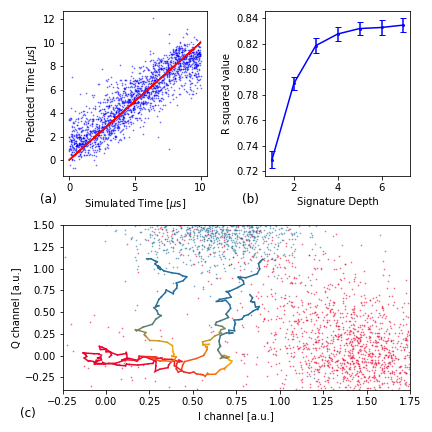
Figure 2: (a) Comparison of simulated transition times with those predicted by an XGBoost regressor Chen and Guestrin (2016) trained on a depth-5 signature. This analysis uses a dataset synthesized from experimental data, and the simulated transition times are considered the ground truth for this prediction task. (b) The coefficient of determination ($r^{2}$ score) of the linear regressor, trained across various signature depths. (c) Prediction of transition points in a trajectory on the experimental data. This plot contains blue and red point blobs, representing the $\ket{0}$ and $\ket{1}$ states, respectively, in a traditional approach for integrating demodulated signals into a single data point. The yellow areas indicate equal probabilities for the $\ket{0}$ and $\ket{1}$ states predicted by the regression, with gradients toward red and blue indicating the likelihood of being in the $\ket{0}$ or $\ket{1}$ state, respectively.

Given the above evidence that signature captures additional information indicating the state transition time, we use signatures as a feature set to train the machine learning models for state classifications on the hardware experimental dataset. The traditional integration approach provides the distribution shown in Fig.4(a). We evaluate the depth-5 path signature using LDA to reduce the number of dimensions to 2, and visualize its distribution in Fig.4(b). We have shown that the $\ket{0}$, $\ket{1}$ and $\ket{2}$ states are more located in a region, especially since the leakage distributions have disappeared. We plot the log-scale histogram of $\ket{0}$ and $\ket{1}$ states in Fig.4(c) and (d) for the integration approach signal and the path signature, respectively.

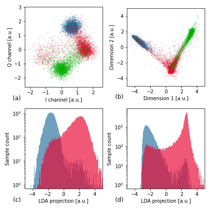
Figure 3: (a) Distribution of experimental dataset on the IQ plane using conventional integration methods. The blue, red and green denotes the state is prepared to $\ket{0}$, $\ket{1}$, and $\ket{2}$ respectively. (b) Projection of a depth-5 signature calculated from the same dataset. The projection direction is evaluated using LDA. (c) Histogram of the integration method projected linearly along the most distinguishable direction using LDA, acting on the data of $\ket{0}$ and $\ket{=1}$ state only. (d) Histogram of signature features (depth=5) from the same dataset, projected similarly.

The performance of the classifier is measured by assignment accuracy, which is the percentage of correctly identified states compared to the intended prepared states. Each method is benchmarked with variations in the cut-off point of the time series provided to the classifier. See Fig.4(e). Our study demonstrates that combining the random forest (RF) algorithm with the signature method surpasses the performance of the conventional approach of integration followed by the Gaussian Mixture Model (GMM). We selected a linear support vector classifier (SVC) and RF for implementing the classification of the signature features. Notably, the RF performs better than linear SVC, which indicates that the signature features between classes are likely not linearly separable. The performance of the random forest model is enhanced when applied to the path signatures, as opposed to directly using the raw trace signals. The above results indicate the effectiveness and added value of incorporating path signatures in the analysis.

Finally, we incorporate an extra post-selection in the dataset, to remove the traces where state transition likely occurred during the measurement. This is done by conducting another measurement immediately after the measurement traces are collected for classification analysis, then applying the traditional integration and the GMM method for readout on the collected signals. See Appendix A for more details. We kept only those traces where the last measurement agreed on the state we intended to prepare. When we applied the signature method to this post-selected dataset, we noted an improvement in accuracy at shorter measurement times. However, this enhancement diminished with longer measurement durations. See Fig.4(f). This outcome leads further evidence to the claim that the signature approach is effective by capturing state transitions occurring during the measurement process.

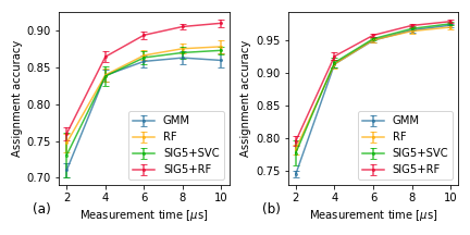
Figure 4: (a) Classification accuracy as a function of measurement length, compared across various classification methods. The tested classification approaches are Gaussian Mixture Model (GMM), Random Forest (RF), Linear support vector classifier on path signature of depth $x$ (SIG$x$+SVC), Random forest on path signature of depth $x$ (SIG$x$+RF) (b) Classification accuracy, excluding state transitions, which is achieved by implementing an extra measurement for post-selection. See supplementary material for more details.

The signature-based features for dispersive readout provide the following benefits: First, the signature approach offers superior accuracy in state discrimination compared to the standard integration and GMM approach. In addition, compared to other machine learning models that directly process the input signal, signatures can be evaluated during the data integration time, which allows the signature method to be efficiently implemented on Field-Programmable Gate Arrays (FPGAs) Lyons (2014a); Chevyrev and Kormilitzin (2016); Fermanian et al. (2023). This efficiency is essential for enabling fast feedback control.

This study has certain limitations. Firstly, the system used for this study does not equip a quantum amplifier, which causes long measurement times. While signatures may be helpful in other aspects than state transition tracking, they are not observable here because the state transition dominates the error. Secondly, our approach employs relatively basic machine learning models. The efficacy of the signature method could potentially be enhanced by integrating more advanced models. However, our focus was on identifying simple models that are easily implementable on FPGAs, thus not delving into more complex machine-learning methods.

In the future, there are a few more directions we can continue research using the path signature approach for improvements of dispersive readout. The first is to combine the signature method with multi-frequency probing, which could provide additional dimensional information Chen et al. (2023), potentially improving readout fidelity further. In addition, this method shows potential in quantum trajectory studies Flurin et al. (2020); van Dorsselaer and Nienhuis (2000) and weak-measurement experiments Flack and Hiley (2014) for accurately analyzing data traces and tracking state changes.

In summary, the signature-based approach offers considerable improvements for dispersive readout. Combined with its potential for tracking the state transition, it can be marked as a valuable tool for quantum technology.

Appendix A Experiment Scheme and Dataset,

The experimental pulse scheme is depicted in Fig.5. It involves three measurements. The qubit state is initially determined using the conventional GMM method, based on data from the first measurement. The traces are then post-selected to ensure that the initial state is the ground state. Subsequently, the qubit is prepared into the $\ket{0}$, $\ket{1}$, and $\ket{2}$ states by applying $\pi$ pulses for the transitions $\ket{0}\rightarrow\ket{1}$ and $\ket{1}\rightarrow\ket{2}$. The gate fidelity is approximately $99.7\%$. A second measurement is conducted afterwards, and the traces are recorded for analysis. Following the second measurement, a third measurement is immediately performed. The third measurement aims to identify any state transitions that occur during the second measurement. Transition events are considered to have occurred if the third measurement yields a state different from the intended preparation state. The state discrimination is implemented with the conventional approach, by applying the GMM model on integrated signals.

Figure 5: Experimental pulse scheme. There are three measurement pulses involved in the experiment. The first measurement is used to implement post-selection, ensuring the initial state is in the ground state. The second measurement pulse is analyzed using the signature approach, while the third measurement is used to detect if a state transition event occurred during the second measurement.

Each trace was acquired using two analog-digital converters with a sampling rate of 1 Gsps each. The traces have two distinct dimensions (I and Q). The recorded signal data has a carrier frequency of 125 MHz. A short-term Fourier transformation was applied to segments of 256 samples to demodulate the signal at this frequency. Samples of the collected traces are shown in Fig.6.

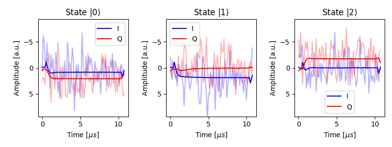
Figure 6: Signal obtained by probing the resonator when the transmon qubit is in states $\ket{0}$, $\ket{1}$, and $\ket{2}$, respectively. The solid line represents the average result, and the translucent line denotes a single-shot example trace. Blue and red colors correspond to the I and Q channels of the signal, respectively.

Using the described experimental scheme, a database was established containing 70,000 traces for each targeted state, culminating in a total of 210,000 traces. The statistics of the post-selection process are presented in the table below. Here, $N_{i}$ represents the number of traces intended for state preparation $\ket{i}$ that pass the initial post-selection, ensuring the initial state is the ground state. $\tilde{N}_{i}$ denotes the number of traces that pass both the initial post-selection and the final post-selection, where the third measurement identifies the state at $\ket{i}$. The ratio $N_{i}/\tilde{N}_{i}$ demonstrates a measure of the proportion of the state that remained unchanged during the second measurement.

Prepared state	$N_{i}$	$\tilde{N}_{i}$	$\tilde{N}_{i}/N_{i}$
$\ket{0}$	$59,768$	$58,273$	$97.50\%$
$\ket{1}$	$52,630$	$32,414$	$61.59\%$
$\ket{2}$	$55,997$	$32,339$	$57.75\%$

For each machine learning classification experiment, 2,000 traces per state were randomly selected from the database, resulting in 6,000 traces per experiment. These traces were then divided into a training set of 4,800 traces and a testing set of 1,200 traces, and the accuracies reported are testing set accuracies. Each hyperparameter configuration was evaluated across 10 repeated experiments with different random seeds for selecting the data from the database and for splitting the training and testing datasets to ensure robust statistical analysis.

Appendix B Experiment Setup

The experiment setup of the readout chain is sub-optimal due to the lack of quantum amplifiers. The detailed readout chain is described in Fig.7.

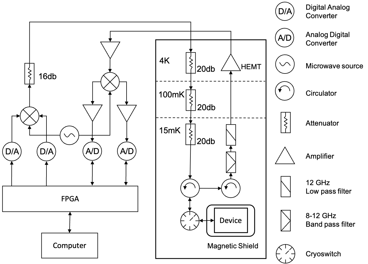
Figure 7: The schematics of the readout chain of the experiment setup.