The Manifold Density Function: An Intrinsic Method for the Validation of Manifold Learning

Abstract

We introduce the manifold density function, which is an intrinsic method to validate manifold learning techniques. Our approach adapts and extends Ripley’s $K$-function, and categorizes in an unsupervised setting the extent to which an output of a manifold learning algorithm captures the structure of a latent manifold. Our manifold density function generalizes to broad classes of Riemannian manifolds. In particular, we extend the manifold density function to general two-manifolds using the Gauss-Bonnet theorem, and demonstrate that the manifold density function for hypersurfaces is well approximated using the first Laplacian eigenvalue. We prove desirable convergence and robustness properties.

Keywords    manifold learning, algorithm validation, Ripley’s $K$-function, hypersurfaces

1 Introduction

Manifold learning is extremely well-studied in the machine learning, computational geometry, and computational topology literatures [17, 19, 39]. The uses of manifold learning, while generally categorized as a means for nonlinear dimensionality reduction [3, 4, 13, 30, 35], span application areas including shape recognition [20], image recognition [40, 5, Ch. 4], and motion planning [11]. Given the large number of techniques and their practical significance, natural questions concerning their validation are raised. That is, when has an algorithm effectively learned manifold structure within data? Moreover, how does one rigorously compare the performance of different manifold learning algorithms? When validating dimensionality reduction algorithms, it is especially pertinent to work in an unsupervised setting. In this paper, we thus assume little or no knowledge of the ground truth in data (such as knowledge of true geodesic distances). Validation in this unsupervised setting is called intrinsic validation, as observations are reliant only on core properties of the presented data.

Despite its prevalence and pivotal role in data analysis, validation techniques specific to manifold learning have been largely unexplored. A manifold analog to Precision-Recall is given in the experimental analysis of [24, Section 3.5]. However, this method requires knowledge of geodesics on the latent manifold and can therefore be considered extrinsic (even though the manifold learning method proposed in [24] is unsupervised). Our work is also related to extensions of Ripley’s $K$-function for spaces more complicated than $\mathbb{R}^{d}$, such as the extension over $\mathbb{S}^{d}$ given in [25]. More recently, Ward et al. develop nonparametric estimation of intensity functions point processes over Riemannian manifolds [38]. However, such methods again rely on knowledge of a ground truth geodesic distance, which is infeasible for most contexts in unsupervised manifold learning. An intrinsic approach is given in [36] which uses persistent local homology to detect singularities in point cloud data. This paper takes a different perspective, giving a global assessment of the manifold properties of data rooted in differential geometry. The advantage of the proposed approach is that it allows for intrinsic validation while making theoretical robustness and complexity guarantees on large classes of Riemannian manifolds.

Contributions

Intuitively, to say that discrete data exhibits “manifold-like” properties could naturally be taken to mean that data locally resembles a uniform sample in $\mathbb{R}^{d}$. This manuscript makes such a notion rigorous. We examine local neighborhoods within a point cloud, scoring how closely each neighborhood resembles a uniform sample in $\mathbb{R}^{d}$ without any knowledge of the ground truth manifold. Our method is based on the natural idea that geodesic balls on a manifold $\mathbb{X}$ should grow proportionately to balls in $\mathbb{R}^{n}$, up to the curvature of $\mathbb{X}$. In this way, our work can be thought of as a manifold analog to the silhouette coefficient for clustering [29]. Specifically, taking inspiration from Ripley’s $K$-function [12], we define a density estimator for manifolds using principles from differential geometry, most notably the Gauss-Bonnet theorem and hypersurface inequalities relating scalar curvature to first Laplacian eigenvalue. In particular, this paper presents the following:

1. We introduce the manifold density function, ${K}_{\mathbb{X}}$, which maintains desirable convergence properties and is exactly computable when the scalar curvature is known.

2. A robust, efficiently computable approximation for ${K}_{\mathbb{X}}$ on two-manifolds with provable accuracy using the Euler characteristic when the latent manifold structure is unknown.

3. A robust, efficiently computable approximation for ${K}_{\mathbb{X}}$ on hypersurfaces with provable accuracy using the first Laplacian eigenvalue when the latent manifold structure is unkown.

The impact of our work is two-fold, providing both an intrinsic manifold validation method and a way to assess the uniformity of data.

2 Background

We begin by providing the requisite definitions from geometry, topology, and statistics.

2.1 Fundamental Definitions From Topology and Geometry

We begin with the definitions from topology and geometry. For an additional discussion, we direct readers to Appendix C.2. Recall that a metric space $(\mathbb{X},d)$ is written as a set $\mathbb{X}$ paired with a distance metric

$$d:\mathbb{X}\times\mathbb{X}\to\mathbb{R}_{\geq 0}.$$

We write $\mathbb{B}_{d}(x,r)$ to denote the open ball of radius $r$ centered at $x\in(\mathbb{X},d)$. For ease of notation, we often write $\mathbb{X}$, with the distance assumed. We say that $\mathbb{X}$ is an $n$-dimensional manifold if, at every point in $\mathbb{X}$, there exists a neighborhood homeomorphic to the unit ball in $\mathbb{R}^{n}$.

In particular, we are interested in Riemannian manifolds in this work. Let $\mathbb{X}$ be a smooth manifold, and let $d:\mathbb{X}\times\mathbb{X}\to\mathbb{R}_{\geq 0}$ be a distance. We say that $(\mathbb{X},d)$ is a Riemannian manifold if $d$ is a Riemannian metric. In this case, $\mathbb{X}$ has a well-defined Lebesgue measure $\mu$ [1, §VII.1], making $(\mathbb{X},d,\mu)$ a metric measure space. For example, shortest-path geodesic distances on $\mathbb{X}$, which we denote by $d_{\mathbb{X}}$, is a Riemannian metric. Core to our methods are uniform samples of a manifold:

Definition 2.1 (Uniformly Sampled Manifold Representation).

Let $\mathbb{X}$ be a manifold with geodesics defined. The geodesic distance function on $\mathbb{X}$ is $d_{\mathbb{X}}:\mathbb{X}\times\mathbb{X}\to\mathbb{R}_{\geq 0}$ where $d_{\mathbb{X}}(x,y)$ denotes the geodesic distance between $x$ and $y$. For a uniform, finite sample $S\subset\mathbb{X}$, we can encode $S$ by pairwise distances within a distance matrix $D\in M^{|S|\times|S|}(\mathbb{R}_{\geq 0})$, with elements $d_{\mathbb{X}}(x,y)\leavevmode\nobreak\ \forall x,y\in S$.

Sometimes, instead of having $D$ itself, we might have an approximation of it (based on neighborhood graphs, for instance), denoted $\widetilde{D}$ throughout this manuscript. In this paper, properties of balls in $\mathbb{R}^{n}$ provide a natural backdrop to study more interesting spaces. It is well known that in Euclidean space, an open ball of radius $r$ under the standard Euclidean metric (denoted $\mathbb{B}_{2}(x,r)$) has volume

$$\operatorname{Vol}(\mathbb{B}_{2}(x,r)):=\frac{\pi^{\frac{n}{2}}}{\Gamma(\frac{n}{2}+1)}r^{n},$$ (1)

where $\Gamma$ is the gamma function. Let $\mathbb{X}$ be a Riemannian manifold. We write the Gaussian curvature at a point $x\in\mathbb{X}$ as $\mathcal{G}(x)$, and the scalar curvature at $x\in\mathbb{X}$ as $\mathcal{S}(x)$. Note that for two-manifolds, $\mathcal{S}(x)=2\mathcal{G}(x)$. We often compare the volume of balls in $\mathbb{R}^{n}$ with balls on curved manifolds, whose relationship is expressed by the following ratio:

Theorem 2.1 (Relation Between Volume and Curvature).

Assume $(\mathbb{X},d_{\mathbb{X}})$ is an $n$-dimensional Riemannian manifold. Let $x\in\mathbb{X}$ be a point with scalar curvature $\mathcal{S}(x)$. The ratio between the volume of the ball $\mathbb{B}_{d_{\mathbb{X}}}(x,r)\subseteq\mathbb{X}$ and the volume of the Euclidean ball $\mathbb{B}_{2}(0,r)\subset\mathbb{R}^{n}$ centered at zero is:

$$\frac{\operatorname{Vol}(\mathbb{B}_{d_{\mathbb{X}}}(x,r))}{\operatorname{Vol}(\mathbb{B}_{2}(0,r))}=1-\frac{\mathcal{S}(x)\cdot r^{2}}{6(n+2)}+o(r^{2}).$$

Theorem 2.1 allows us to inspect the relationship between volume and curvature in Riemannian manifolds, and is proven in classical textbooks, including [15, p. 168] and [6, p. 317]. Likewise, the seminal Gauss-Bonnet theorem describes the relationship between the total curvature of $\mathbb{X}$ and its topology.

Theorem 2.2 (Gauss-Bonnet[23]).

Let $\mathbb{X}$ be a compact Riemannian two-manifold, and let $x\in\mathbb{X}$. Then, the total curvature on $\mathbb{X}$ is $\int_{\mathbb{X}}\mathcal{G}dA=2\pi\chi(\mathbb{X})$, where $dA$ is the area element on $\mathbb{X}$ and $\chi(\mathbb{X})$ is the Euler characteristic.

In higher dimensions, generalizations of the Gauss-Bonnet theorem become much more intricate and are only defined for even dimensions. Hence, in dimensions larger than two, we use properties of the total mean curvature of submanifolds of $\mathbb{R}^{n}$, given in [7]. In particular, we relate scalar curvature, mean curvature, and the second fundamental form using the Gauss-Codazzi equations for hypersurfaces; see Appendix C.4 for definitions.

Theorem 2.3 (Gauss-Codazzi Equations for Hypersurfaces [16]).

Let $\mathbb{X}$ be an $n$-dimensional Riemannian manifold immersed in $\mathbb{R}^{m}$. Then, the scalar curvature $\mathcal{S}$ of $\mathbb{X}$ at a point $p\in\mathbb{X}$ is expressed by $\mathcal{S}=H^{2}-||h||^{2}$, where $H$ is the mean curvature of $\mathbb{X}$ at $p$, and $h$ is the second fundamental form of $\mathbb{X}$ at $p$; see Definition C.9.

2.2 Fundamental Definitions from (Spatial) Statistics

Let $(\mathbb{X},d,\mu)$ be a metric measure space; that is, $\mathbb{X}$ is a topological space, $S\subset\mathbb{X}$, $d\colon S\times S\to\mathbb{R}$ is a metric, and $\mu$ is a measure over a suitable collection of subsets of $\mathbb{X}$. Then, let $X=\{X_{i}\}_{i=1}^{m}$ be $m$ samples drawn iid from the uniform distribution over $S$. Let $A$ be a measurable subset of $S$, and, for each $i$, let $A_{i}$ be the random variable that is one if $X_{i}\in A$ and zero otherwise. Since each $X_{i}$ is drawn iid from the uniform distribution over $S$, we know that in any realization of $X$, the expected number of points landing in $A$ is:

$$\mathbb{E}\left[\#(X\cap A)\right]=\sum_{i=1}^{m}\mathbb{E}\left[A_{i}\right]=\sum_{i=1}^{m}\mathbb{P}\left[X_{i}\in A\right]=\frac{m\mu(A)}{\mu(S)}.$$ (2)

Similar to the Buffon needle problem (e.g., [31, pp. 71-2]), we can use this property to estimate geometric properties of $S$ (and of $A$) using the law of large numbers.

Example 2.1 (Estimating Areas).

Consider $A\subseteq S\subset\mathbb{R}^{2}$, such that both $S$ and $A$ are Lebesgue-measurable. Then, for $m$ sufficiently large, the number of points that land in $A$ is approximately the ratio of the area of $A$ to the area of $S$:

$$\left|A\cap X\right|\approx\frac{m\cdot\operatorname{\operatorname{Vol}}\left(A\right)}{\operatorname{\operatorname{Vol}}\left(\mathbb{X}\right)}.$$ (3)

Multiplying both sides by $\operatorname{Vol}(\mathbb{X})$, we see that $\operatorname{\operatorname{Vol}}(A)\approx\frac{m_{A}}{m}\cdot\operatorname{\operatorname{Vol}}(\mathbb{X})$, where $m_{A}$ denotes the number of sample points that land in $A$. So, if we know $\operatorname{\operatorname{Vol}}(S)$, we can use a realization of $X$ to estimate $\operatorname{\operatorname{Vol}}(A)$. This generalizes to Reimannian manifolds.

We note here that this only holds if the points are sampled iid from the uniform distribution over $S$. If the points are sampled from some other distribution, then this area estimation technique would not work for all measurable subspaces $A$. Additionally, the above construction is related to Ripley’s $K$-function, which assesses the homogeneity of point processes. Let $S\subset\mathbb{R}^{d}$ be compact and Lebesgue-measurable, containing the subset $S_{R}=\{x\in S|d_{2}(x,\partial S)\leq R\}$. In particular, our formulation is related to the special case when a point process is drawn iid from a uniform distribution, which results in the $K$-function $\mathcal{K}:[0,R]\to\mathbb{R}$ defined by

$$\mathcal{K}_{p}(r)=\operatorname{Vol}(\mathbb{B}_{L_{2}}(p,r)),$$

for a range of radii $[0,R]$ and a point $p$ sampled uniformly from $S\subset\mathbb{R}^{d}$. The theoretical $K$-function is estimated with empirical versions; for more details and a rigorous definition we refer readers to Appendix B.

2.3 Manifold Learning and Validation

Having given the definitions relevant to manifolds themselves, we lay out the paradigm on manifold learning and its validation. Broadly speaking, manifold learning operates on the assumption that data is sampled uniformly from a manifold $\mathbb{X}$, and attempts to learn $\mathbb{X}$ by approximating geodesic distances [14, 26]. Because of the variety in approaches, there is no agreed-upon definition of a manifold learning algorithm. We give a general definition of manifold learning that will be used throughout this work, which is informed by the core structures of manifolds themselves. That is, we consider arbitrary manifold learning methods as a map from set of data to a distance matrix:

Definition 2.2 (Manifold Learning).

A manifold learning model $F\colon S\to M^{|S|\times|S|}(\mathbb{R}_{\geq 0})$ is a map from a set of data $S$ (assumed to be sampled uniformly from an $n$-dimensional ambient manifold) to an $|S|\times|S|$ real-valued distance matrix. We can think of $F$ as a map approximating geodesic distances, so we typically write $F(S)=\widetilde{D}$, and we write $D$ as the true geodesic distance matrix for all points of $S$.

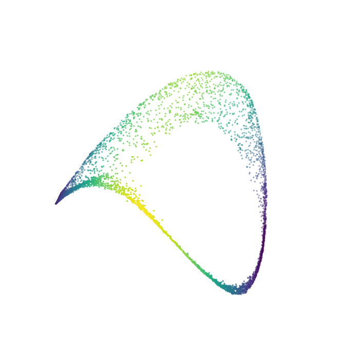
Figure 1: Constructing 3D embeddings of a Klein bottle lifted in ten dimensions, with varying success. From left to right, an output from PCA, ISOMAP, t-SNE, LLE, and spectral embedding. From visual inspection, PCA appears to have performed best in this example, followed by ISOMAP.

It should be noted that many manifold learning techniques compute an embedding rather than a distance matrix, wherein geodesics are implicit. In such cases, we can compute a geodesic distance matrix by constructing a neighbor graph in the space of the embedding and computing graph distances in a similar manner to the ISOMAP algorithm of [35]. We refer the readers to [19, 39, 17] for descriptions of many different manifold learning techniques and frameworks. Generally, our paper considers manifold learning in an unsupervised setting, assuming no knowledge of the ground truth geodesic distances, $D$. In this setting, validation must be done using properties intrinsic to the “learned manifold” approximated by $\widetilde{D}$ alone. In general, intrinsic validation approaches have been quite successful in other areas of machine learning, for example silhouette coefficients for clustering [29], which rely only on properties intrinsic to clusters themselves.

3 An Intrinsic Manifold Validation Method

Let $(\mathbb{X},d_{\mathbb{X}})$ be a Riemannian $n$-manifold. Let $X\subset\mathbb{X}$ be a uniform sample on $\mathbb{X}$ By Theorem 2.1, for $x\in\mathbb{X}$ and $r>0$, we can write the volume of a ball $\mathbb{B}_{2}(0,r)$ in $\mathbb{R}^{n}$ as a function of the scalar curvature at $x$ and the volume of the ball $\mathbb{B}_{d_{\mathbb{X}}}(x,r)$ in $\mathbb{X}$:

$$\operatorname{Vol}(\mathbb{B}_{2}(0,r))=\frac{\operatorname{Vol}(\mathbb{B}_{d_{\mathbb{X}}}(x,r))}{(1-\frac{\mathcal{S}(x)\cdot r^{2}}{6(n+2)}+o(r^{2}))}.$$ (4)

Furthermore, if $\operatorname{Vol}{\mathbb{X}}$ is known, we can estimate By Equation (2) and the law of large numbers, we know that if $|X|$ is sufficiently large, then the number of points landing in any measurable region $A\subset\mathbb{X}$ is approximately $\frac{m\operatorname{Vol}(A)}{\operatorname{Vol}(\mathbb{X})}$. Thus, if we know $\operatorname{Vol}(\mathbb{X})$, we can estimate $\operatorname{Vol}(A)$, and vice versa. Putting these two observations together, we define the manifold density function:

Definition 3.1 (Manifold Density Function And Its Estimators).

Let $(\mathbb{X},d_{\mathbb{X}})$ be a Riemannian $n$-manifold, and let $X\subset\mathbb{X}$ be a uniform sample on $\mathbb{X}$. Let $p\in\mathbb{X}$, and let $R>0$ be sufficiently small. Then, the manifold density function is the function ${K}_{\mathbb{X}}\colon[0,R]\to\mathbb{R}$ defined by

$${K}_{\mathbb{X}}(r):=\frac{\operatorname{Vol}(\mathbb{B}_{2}(0,r))}{\operatorname{Vol}(\mathbb{X})}$$ (5)

with local estimator $\widehat{K}_{p}\colon[0,R]\to\mathbb{R}$ defined by

$$\widehat{K}_{p}(r):=\left(1-\frac{\mathcal{S}(p)\cdot r^{2}}{6(n+2)}\right)^{-1}\cdot\frac{1}{|X|}\sum_{x\in X}I(x\in B_{r}(p))$$ (6)

and an aggregated estimator $\widehat{K}\colon[0,R]\to\mathbb{R}$ defined by

$$\widehat{K}(r):=\frac{1}{|X|^{2}}\sum_{p\in X}\left(\left(1-\frac{\mathcal{S}(p)\cdot r^{2}}{6(n+2)}\right)^{-1}\cdot\sum_{x\in X}I(x\in B_{r}(p))\right)$$ (7)

If $\mathbb{X}$ is flat, then $\mathcal{S}(p)=0$, simplifying $\widehat{K}_{p}$ and $\widehat{K}$. That is, we remove the first term of $\widehat{K}_{p}$ and $\widehat{K}$, giving $\widehat{K}_{p}(r):=\frac{1}{|X|}\sum_{x\in X}I(x\in B_{r}(p))$ and $\widehat{K}(r):=\frac{1}{|X|^{2}}\sum_{p\in X}\sum_{x\in X}I(x\in B_{r}(p))$. Notice that the manifold density function is indeed related to Ripley’s $K$-function in the special case for uniform samples, in which case the two vary by only the factor $1/\text{Vol}(\mathbb{X})$ in the theoretical setting and $1/|X|$ in the empirical formulation.

3.1 The Manifold Score

We call the $L_{2}$-distance between a function and its estimate, for example, $||{K}_{\mathbb{X}}-\widehat{K}||_{2}$, the error of the estimate. Since the estimators drop an $o(r^{2})$ term from Equation (4), we note that $\widehat{K}_{p}$ and $\widehat{K}$ are biased estimators of ${K}$; that is, for all $r\geq 0$, we have $\widehat{K}_{p}(r)\geq{K}(r)$ and there exists cases where equality doesn’t hold.

Finally, we define a score by taking a simple normalization of the error of an estimator of ${K}_{\mathbb{X}}$.

Definition 3.2 (Manifold Score).

Let $\mathbb{X}$ be a compact Riemannian manifold, and $X\subset\mathbb{X}$ a finite sample. The local manifold score for $X$ as representing the manifold $\mathbb{X}$ at $p\in X$ is

$$M_{p}(X)=1-\frac{1}{|X|}||{K}_{\mathbb{X}}-\widehat{K}_{p}||_{2},$$ (8)

and the aggregated manifold score is

$$M(X)=1-\frac{1}{|X|}||{K}_{\mathbb{X}}-\widehat{K}||_{2}.$$ (9)

This score indicates the extent to which a sample resemples a uniformaly distributed set of points on a manifold.

We note that manifold density function is well-defined and normalized, leaving verification for the appendix. From this structure, a manifold score of one indicates a perfectly uniform sample, and a manifold score of one indicates a perfectly nonuniform sample, likely differentiating between an effective and ineffective manifold-learning scheme.

3.2 Manifold Density Functions For Manifolds With Curvature

We now introduce a primary theoretical result of the paper, adapting the manifold density function to manifolds with curvature. We begin with a brief discussion of local manifold density functions and their shortcomings. Related extensions for Ripley’s $K$-function to more general settings have been attempted before, and include extensions for spheres [22, 37], and for fibers [32]. We present the first extension of its kind for general Riemannian two-manifolds and hypersurfaces, which in the aggregated setting can be made entirely intrinsic.

At its core, our approach is designed with the specific intent to assess the uniformity of a sample lying on arbitrary manifolds rather than within Euclidean space alone. By its very formulation, for an arbitrary point $p$ on a Riemannian manifold $\mathbb{X}$, the local manifold density function is defined in terms of the scalar curvature $\mathcal{S}(p)$ at $p$. If we are equipped with knowledge of $\mathcal{S}(p)$ at $p$, then we can compute the local manifold density function directly. A straightforward but desirable consequence of this definition is the following theorem, allowing us to understand the local manifold density function in terms of Euclidean balls:

Theorem 3.1.

Let $\mathbb{X}$ be a compact Riemannian manifold, and let $X\subset\mathbb{X}$ be a uniform sample on $\mathbb{X}$. Let $p\in X$. Then, for sufficiently small $r>0$ and large $|X|$, $\widehat{K}_{p}(r)$ converges to the theoretical manifold density function ${K}_{\mathbb{X}}(r)$.

Proof.

Expanding definitions,

$$\widehat{K}_{p}(r) =\left(1-\frac{\mathcal{S}(p)\cdot r^{2}}{6(n+2)}\right)^{-1}\cdot\frac{1}{|X|}\sum_{x\in X}I(x\in B_{r}(p))$$ (10)

$$=\frac{\text{Vol}(\mathbb{B}_{2}(0,r))}{\text{Vol}(\mathbb{B}_{\mathbb{X}}(r,x))}\cdot\frac{1}{|X|}\sum_{x\in X}I(x\in B_{r}(p))\text{ for sufficiently small $r$}$$ (11)

$$\to\frac{\text{Vol}(\mathbb{B}_{2}(0,r))}{\text{Vol}(\mathbb{B}_{\mathbb{X}}(r,x))}\cdot\frac{\text{Vol}(\mathbb{B}_{\mathbb{X}}(r,x))}{\text{Vol}(\mathbb{X})}\text{ by the law of large numbers}$$ (12)

$$=\frac{\text{Vol}(\mathbb{B}_{2}(0,r))}{\text{Vol}(\mathbb{X})}={K}_{\mathbb{X}}(r).$$ (13)

Where we estimate area by sampling on Riemannian manifolds, see Example 2.1. It follows that $\widehat{K}_{p}(r)$ converges to ${K}_{\mathbb{X}}{(r)}$ for large sample size $|X|$, and sufficiently small $r$. ∎

The same derivation can be used for Ripley’s $K$-function in the uniform case, dropping the $1/|X|$ term. However, one should note that there are a few undesirable properties that go along with Definition 3.1 in the local setting. Most notably, our focus is on intrinsic validation, and knowing the scalar curvature at any point $p\in X$ violates the true spirit of an intrinsic method. Additionally, Theorem 2.1 only technically holds for balls with sufficiently small radius $r>0$, and the equation in general incurs an additive error term $o(r^{2})$. As such, the scaling in Definition 3.1 becomes less accurate in approximating ${K}_{\mathbb{X}}$ as $r$ increases. The latter problem can be mitigated by considering small enough radii (although an exact bound on the error term remains a difficult and manifold-specific problem in differential geometry), and the former is resolved by considering global properties of the aggregated manifold density function.

3.3 Aggregated Manifold Density Functions for Surfaces

Let $\mathbb{X}$ a compact Riemannian two-manifold, and let $X\subset\mathbb{X}$ be a uniform sample of $X$. In the aggregated setting, since $\widehat{K}$ is a global average of every manifold density function on $X$, we are able to avoid the shortcomings in the local setting by exploiting fundamental results in differential geometry. Namely, we first recall Theorem 2.2, the Gauss-Bonnet theorem, which categorizes the relationship between geometry and topology for two-manifolds, establishing that the total curvature of a manifold is a function of its Euler characteristic. In addition, we recall that the scalar curvature at a point $p\in\mathbb{X}$ on a two-manifold is twice the Gaussian curvature: $\mathcal{G}(p)=2\mathcal{S}(p)$. Considering the total curvature over all of $\mathbb{X}$ and the ratio given in Theorem 2.1, we can relate the total area of balls of radius $r>0$ in $\mathbb{X}$ to the total volume of radius $r$ balls in $\mathbb{R}^{2}$ for sufficiently small $r$.

Lemma 3.1 (Average Volume Distortion of Balls).

Let $\mathbb{X}$ be a compact Riemannian two-manifold. On average, the ratio $\frac{\text{Vol}(\mathbb{B}_{\mathbb{X}}(p,r))}{\text{Vol}(\mathbb{B}_{2}(0,r))}$ between the volume of $L_{2}$ and geodesic balls for a point $p\in\mathbb{X}$ is

$$1-\frac{\pi\chi(\mathbb{X})}{24\cdot A}\cdot r^{2}+o(r^{2}),$$

where $A$ is the area form of $\mathbb{X}$ and $\chi(\mathbb{X})$ is the Euler characteristic.

Proof.

We expand definitions and integrate over the area form $dA$ of $\mathbb{X}$:

$$\frac{1}{A}\int_{\mathbb{X}}\frac{\text{Vol}(\mathbb{B}_{d_{\mathbb{X}}}(x,r))}{\text{Vol}(\mathbb{B}_{2}(0,r))}dA =\frac{1}{A}\left[A-\int_{\mathbb{X}}\frac{\mathcal{S}(x)}{6(n+2)}\cdot r^{2}dA+Ao(r^{2})\right]\text{ by Equation\leavevmode\nobreak\ (\ref{eq:euclidballest})}$$ (14)

$$=1-\frac{1}{A}\int_{\mathbb{X}}\frac{\mathcal{G}(x)}{48}\cdot r^{2}dA+o(r^{2})$$ (15)

$$=1-\frac{\pi\chi(\mathbb{X})}{24\cdot A}\cdot r^{2}+o(r^{2}),$$ (16)

giving a formula for the average ratio between the volume of Euclidean and geodesic balls in terms of the Euler characteristic, accompanied by an error term with value $o(r^{2})$. ∎

This gives canonically an approximation dependent only on the Euler characteristic.

Lemma 3.2 (Approximate Ratio for Surfaces).

Let $\delta=\frac{r^{2}}{A}$ and $\epsilon=o(r^{2})$, the additive error. Then we can estimate the left hand side of Lemma 3.1 with $1-\frac{\pi\chi(\mathbb{X})}{24}$, which gives the approximation:

$$\left|\frac{1}{A}\int_{\mathbb{X}}\frac{\text{Vol}(\mathbb{B}_{d_{\mathbb{X}}}(x,r))}{\text{Vol}(\mathbb{B}_{2}(0,r))}dA-1-\frac{\pi\chi(\mathbb{X})}{24}\right|\leq\frac{(1-\delta)\chi(\mathbb{X})}{24}+\epsilon.$$

Proof.

From Lemma 3.1, $\frac{1}{A}\int_{\mathbb{X}}\frac{\text{Vol}(\mathbb{B}_{d_{\mathbb{X}}}(x,r))}{\text{Vol}(\mathbb{B}_{2}(0,r))}dA=1-\delta\frac{\pi\chi(\mathbb{X})}{24}+\epsilon$, giving

$$\left|\left(1-\delta\frac{\pi\chi(\mathbb{X})}{24}-\epsilon\right)-\left(1-\frac{\pi\chi(\mathbb{X})}{24}\right)\right|\leq|(\delta-1)\frac{\pi\chi(\mathbb{X})}{24}|+|-\epsilon|$$

by the triangle inequality, which equals $(1-\delta)\frac{\pi\chi(\mathbb{X})}{24}+\epsilon$ since $\delta\leq 1$ and $\epsilon>0$. ∎

We thus have a definition of total area distortion due to curvature on a two-manifold, which informs our scaling procedure of the aggregated manifold density function on a two-manifold. Namely, as a consequence of Lemma 3.1, the aggregated manifold density function on a general two-manifold with curvature is invariant of its Euler characteristic, and converges to the standard manifold density function as the sample size increases:

Theorem 3.2.

Let $\mathbb{X}$ be a compact Riemannian two-manifold, and let $X\subset\mathbb{X}$ be a uniform sample on $\mathbb{X}$. For large $|X|$ and sufficiently small $r>0$, $\widehat{K}(r)$ converges to ${K}_{\mathbb{X}}(r)$.

Proof.

We examine the result of Theorem 3.1 when considered globally on $\mathbb{X}$.

$$\widehat{K}(r) =\frac{1}{|X|^{2}}\sum_{p\in X}\left(\left(1-\frac{\mathcal{S}(p)\cdot r^{2}}{6(n+2)}\right)^{-1}\cdot\sum_{x\in X}I(x\in B_{r}(p))\right)$$

$$\to\frac{1}{A^{2}}\int_{\mathbb{X}}\frac{\text{Vol}(\mathbb{B}_{d_{\mathbb{X}}}(p,r))dA}{(1-\frac{\mathcal{S}(p)}{6(n+2)}*r^{2})}\text{ for large $|X|$}$$

$$\to\frac{1}{A^{2}}\int_{\mathbb{X}}\operatorname{Vol}(\mathbb{B}_{2}(0,r))dA\text{ for small enough $r$, by Equation\leavevmode\nobreak\ (\ref{eq:euclidballest})}$$

$$=\frac{\operatorname{Vol}(\mathbb{B}_{2}(0,r))}{A^{2}}\cdot A=\text{Vol}(\mathbb{B}_{2}(0,r))/A={K}_{\mathbb{X}}(r).$$

Where we integrate over the area form $A$ of $\mathbb{X}$. Moreover, the second to last equality follows from the fact that the volume of Euclidean balls $\operatorname{Vol}(\mathbb{B}_{2}(0,r))$ is taken as a constant over $\mathbb{X}$ for a fixed radius $r$, and thus we integrate only over $dA$. Hence, for large $|X|$, $\widehat{K}(r)\to{K}_{\mathbb{X}}(r)$. ∎

Examining the integral in the denominator of Line 2 in Theorem 3.2 gives a strong approximation of the aggregated manifold density function $\widehat{K}$ on a surface, which depends on the global topology of $\mathbb{X}$ due to the Gauss-Bonnet theorem and making use of the fact that $\mathcal{G}(p)=2\mathcal{S}(p)$ for surfaces:

Corollary 3.1.

Let $\mathbb{X}$ be a compact Riemannian manifold, and let $X\subset\mathbb{X}$ be a uniform sample on $\mathbb{X}$. We approximate:

$$\widehat{K}(r):=\left(1-\frac{\pi\chi(\mathbb{X})\cdot r^{2}}{24A}\right)^{-1}\cdot\frac{1}{|X|^{2}}\sum_{p\in X}\left(\sum_{x\in X}I(x\in B_{r}(p))\right)$$

Then as $|X|$ increases, $\widehat{K}(r)\to{K}_{\mathbb{X}}(r)$. Moreover, taking $A=O(r^{2})$, we have the approximation dependent only on the Euler characteristic:

$$\widehat{K}(r):=\left(1-\frac{\pi\chi(\mathbb{X})}{24}\right)^{-1}\cdot\frac{1}{|X|^{2}}\sum_{p\in X}\left(\sum_{x\in X}I(x\in B_{r}(p))\right)$$

Consequently, in the aggregated setting we scale the average of local manifold density functions by a function of the Euler characteristic and the area of $\mathbb{X}$. In fact, as we demonstrate experimentally, the heuristic approximation of $\widehat{K}(r)$ given by taking $A=O(r^{2})$ is typically sufficient, allowing us to scale the manifold density function using the Euler characteristic alone. Assuming no knowledge of the Euler characteristic, we can simply estimate $\chi(\mathbb{X})$ by selecting an integer that minimizes $M(\widehat{K}(r))$.

3.4 Aggregated Manifold Density Functions in High Dimensions

As is indicated by the ratio given in Theorem 2.1, the volume form of a Riemannian manifold $\mathbb{X}$ depends on the scalar curvature, and in two dimensions we are able to use the Gauss-Bonnet theorem alone due to the direct relation between $\mathcal{S}(x)$ and $\mathcal{G}(s)$ on surfaces. Unfortunately, higher-dimensional generalizations of the Gauss-Bonnet theorem rely on the Pfaffian of $\mathbb{X}$, which is a function of Ricci, Riemannian, and scalar curvature. Instead, we scale the aggregated manifold density function by a different global constant of manifolds, namely $\lambda_{1}$, the first eigenvalue of their Laplacian operator. We focus our attention where bounds to $\lambda_{1}$ are known, thus dealing with orientable, compact hypersurfaces. In particular, two useful bounds on $\lambda_{1}$ are given by the following theorems, which relate $\lambda_{1}$ to the mean curvature $H$, and to the squared length of the second fundamental form $h$. See Appendix C.4 for more details.

Theorem 3.3 (Total Mean Curvature [7]).

Let $\mathbb{X}$ be an $n$-dimensional, compact submanifold in $\mathbb{R}^{m}$, and $H$ the mean curvature at any point $p\in\mathbb{X}$. Then

$$\int_{M}|H|^{k}dV\leq\left(\frac{\lambda_{q}}{n}\right)^{\frac{k}{2}}\text{Vol}(\mathbb{X}),$$

where $\lambda_{q}$ denotes the $q$th Eigenvalue of the Laplacian operator.

In addition, the length of $h$ is related to $\lambda_{1}$ in the following way:

Theorem 3.4 (Total Length of the Second Fundamental Form [7]).

Let $\mathbb{X}$ be a compact orientable $n$-dimensional submanifold of $\mathbb{R}^{m}$ with arbitrary codimension. Then,

$$\int_{\mathbb{X}}||h||^{2}dV\geq\lambda_{1}\text{Vol}(\mathbb{X}).$$

Equipped with these results, we have a mechanism to scale manifold density functions in higher dimensions. Let $\mathbb{X}$ be a compact, $n$-dimensional orientable manifold embedded in $\mathbb{R}^{n+1}$, i.e., $\mathbb{X}$ is a hypersurface in Euclidean space. Let $r>0$, where $r$ is sufficiently small to satisfy the ratio given in Theorem 2.1. As was done in Section 3.3, we compute the ratio of the total volume of balls of radius $r$ on $\mathbb{X}$ to the total volume of balls of radius $r$ in $\mathbb{R}^{n}$. The following integral is taken over the volume form $dV$ of $\mathbb{X}$, given formally in Appendix C.3:

$$\int_{\mathbb{X}}\frac{\text{Vol}(\mathbb{B}_{d_{\mathbb{X}}}(x,r))}{\text{Vol}(\mathbb{B}_{2}(0,r))}dV =\text{Vol}(\mathbb{X})-\int_{\mathbb{X}}\frac{\mathcal{S}(x)}{6(n+2)}\cdot r^{2}dV+\text{Vol}(\mathbb{X})o(r^{2})$$

$$=\text{Vol}(\mathbb{X})-\int_{\mathbb{X}}\frac{H^{2}-||h||^{2}}{6(n+2)}\cdot r^{2}dV+\text{Vol}(\mathbb{X})o(r^{2})\text{ (by Theorem\leavevmode\nobreak\ \ref{thm:gc-eqn})}$$

$$=\text{Vol}(\mathbb{X})-\frac{r^{2}}{6(n+2)}\left(\int_{\mathbb{X}}H^{2}dV-\int_{\mathbb{X}}||h||^{2}dV\right)+\text{Vol}(\mathbb{X})o(r^{2}).$$

Now, notice from Theorem 3.3 and Theorem 3.4:

$$\int_{\mathbb{X}}H^{2}dV-\int_{\mathbb{X}}||h||^{2}dV\leq\frac{\lambda_{1}}{n}\text{Vol}(\mathbb{X})-\lambda_{1}\text{Vol}(\mathbb{X}).$$

This leads to the following approximation for the average ratio between geodesic and $L_{2}$ balls:

$$\frac{1}{\text{Vol}(\mathbb{X})}\int_{\mathbb{X}}\frac{\text{Vol}(\mathbb{B}_{d_{\mathbb{X}}}(x,r))}{\text{Vol}(\mathbb{B}_{2}(0,r))}dV$$

$$\approx 1-\frac{r^{2}}{6(n+2)\text{Vol}(\mathbb{X})}\left(\frac{\lambda_{1}}{n}\text{Vol}(\mathbb{X})-\lambda_{1}\text{Vol}(\mathbb{X})\right)+o(r^{2})$$

$$=1-\left(\frac{r^{2}\cdot\lambda_{1}(1-n)}{6(n)(n+2)}\right)+o(r^{2})$$

More specifically, the above substitution is a $(2+1/n)$-approximation for the true value.

Lemma 3.3 (Hypersurface Approximation Factor).

The difference $B=\int_{\mathbb{X}}H^{2}dV-\int_{\mathbb{X}}||h||^{2}dV$ and its approximation $A=\frac{\lambda_{1}}{n}\text{Vol}(\mathbb{X})-\lambda_{1}\text{Vol}(\mathbb{X})$ satisfy $|B-A|\leq(2+1/n)|B|$.

Proof.

Both $\int_{\mathbb{X}}H^{2}dV,\int_{\mathbb{X}}||h||^{2}dV\geq 0$ and $A=\frac{1-n\lambda_{1}}{n}\text{Vol}(\mathbb{X})\leq 0$, implying $\frac{1}{n}\int_{\mathbb{X}}||h||^{2}dV\geq\int_{\mathbb{X}}H^{2}dV$. This implies $|B|\leq\int_{\mathbb{X}}||h||^{2}dV\leq\frac{\lambda_{1}}{n}\text{Vol}(\mathbb{X})+|B|\leq(1+\frac{1}{n})|B|$. Moreover, since $|A|=|\frac{(1-n)\lambda_{1}}{n}\text{Vol}(\mathbb{X})|\leq\lambda_{1}\text{Vol}(\mathbb{X})\leq\int_{\mathbb{X}}||h||^{2}dV$, it follows that $|B|+|-A|\leq(2+1/n)|B|$. By the triangle inequality, $|B-A|\leq(2+1/n)|B|$ as desired. ∎

Which obtains a desired analog for hypersurfaces scaling manifold density function using $\lambda_{1}$.

Definition 3.3 (Hypersurface Aggregated Manifold Density Function).

Let $\mathbb{X}$ a compact, orientable Riemannian $n$-manifold immersed in $\mathbb{R}^{n+1}$, and let $X\subset\mathbb{X}$ be a uniform sample of $\mathbb{X}$. The aggregated manifold density function for hypersurfaces $\widehat{K}(r)$ is approximated by:

$$\widehat{K}(r)\approx\left(1-\frac{r^{2}\cdot\lambda_{1}(n-1)}{12(n)(n+2)}\right)^{-1}\cdot\frac{1}{|X|^{2}}\sum_{p\in X}\left(\sum_{x\in X}I(x\in B_{r}(p))\right)$$

It follows from Lemma 3.3 and Definition 3.1 that Definition 3.3 attains a small multiplicative approximation factor, coupled with the standard additive error.

Corollary 3.2 (Approximation Factor for Definition 3.3).

Let $\widehat{K}(r)$ be as approximated above, then if $|X|$ is uniformly sampled from $\mathbb{X}$, we have $|{K}_{\mathbb{X}}-\widehat{K}(r)|\leq(2+1/n)\left(\frac{r^{2}\cdot\lambda_{1}(n-1)}{12(n)(n+2)}\right)^{-1}+\epsilon$ where ${K}_{\mathbb{X}}$ is the theoretical manifold density function and $\epsilon=o(r^{2})$ is the error of Theorem 2.1.

Note that for many common hypersurfaces, $\lambda_{1}$ is either known, or there exists a “reasonable” approximation; see Appendix C.5 for examples. Given any fundamental knowledge of the ambient hypersurface, (e.g., if $\mathbb{X}$ can reasonably be assumed to lie on a hypersphere, or similar manifold), we choose $\lambda_{1}$ explicitly from the known approximations. Otherwise, analogously to tuning the manifold density function by choosing the Euler characteristic $\chi(\mathbb{X})$ minimizing $M(\widehat{K})$, we choose the approximation for $\lambda_{1}$ minimizing $M(\widehat{K})$.

4 Desiderata

We remark on desirable properties when validating algorithms in machine learning, and assess the computational complexity, robustness, and intrinsic properties of our technique.

4.1 Robustness

It is pertinent when attempting the validation of random samples to achieve stability against noise. Given a sample $X\subset\mathbb{X}$ on a (flat or curved) Riemannian manifold $\mathbb{X}$, this implies that subjecting a point $p\in X$ to small perturbation $\delta>0$ should change the validation score of $M(p)$ very little. We thus examine the local and aggregated manifold scores $M(\widehat{K}_{p})$ and $M({K}_{\mathbb{X}})$ with respect to their stability after subjecting points of $X$ to noise. In the aggregated setting, it is not difficult to make robustness guarantees about the manifold density function. Specifically, for a point $p\in X$, examine $p\pm\delta$. Indeed, for a fixed radius $r>0$, in the worst case, $\widehat{K}_{p}(r)$ could change at most by $|X|$, and for every other $p^{\prime}\not=p\in\mathbb{X}$, $\hat{K}_{p^{\prime}}(r)$ could change by at most $1$. This alters the aggregated manifold density function, ${K}_{\mathbb{X}}$, by at most $\pm 2/|X|$. However, a small change by $\delta$ to $r$ gives the identical manifold density function prior to the perturbation, i.e., $\hat{K}_{p}(r\pm\delta)=\hat{K}_{p}(r)$. The worst-case bound remains the same if we allow perturbations of every $p\in\mathbb{X}$ by $0\leq\delta^{\prime}\leq\delta$ for both ${K}_{\mathbb{X}}$ and $\widehat{K}_{p}(r)$ when considering a fixed radius $r$. Hence, we can consider the aggregated manifold density function to be resistant to noise for fixed radii, and both the local and aggregated manifold density functions can be considered resistant to noise when allowing a change in radius $r\pm\delta$. Consequently, our manifold score $M({K}_{\mathbb{X}})$ is robust to noise up to the equivalent thresholds.

4.2 Computation

Let $X\subset\mathbb{X}$, where $\mathbb{X}$ is an $n$-dimensional Riemannian manifold with $|X|=m$. Using our construction, adjusting the computation of the aggregated manifold density function to arbitrary manifolds only adds a constant factor in runtime complexity under reasonable assumptions about the complexity of a manifold and the dimension. For surfaces, assuming that $\chi(\mathbb{X})$ is a fixed constant, we could have $O(1)$ manifold density function estimations, each of which adds only an $O(1)$ factor in finding the value for $\chi(\mathbb{X})$ minimizing $M({K}_{\mathbb{X}})$. For hypersurfaces, again we search over $O(1)$ known formulas for $\lambda_{1}$, each of which scale computation of ${K}_{\mathbb{X}}$ by an $O(1)$ factor. Assuming the dimension is $O(d)$, we can use the same procedure to naively compute the dimension minimizing $M({K}_{\mathbb{X}})$, adding only an $O(d)$ factor to the complexity. Given an algorithm to compute Ripley’s $K$-function, we can compute manifold density function adding only an $O(1)$ factor, when the values of $d,\chi(\mathbb{X})$, and $\lambda_{1}$ are constant. Naively, computing the manifold density function in either the aggregated or disaggregated settings are computed in $\Theta(n^{2})$ time. More efficient implementations are likely possible by efficiently embedding the given distance matrix in $\mathbb{R}^{n}$, and then using an $n$-dimensional range tree to compute $\widehat{K}_{p}(r)$ for a given radius $r$. Doing so is possible in $O(\log^{n-1}m+k)$ time using fractional cascading, where $k=\widehat{K}_{p}(r)$. Finding ${K}_{\mathbb{X}}$ overall is done by computing $\widehat{K}_{p}(r)$ for every $p\in X$, which takes $O(m(\log^{n-1}m+k_{max}))$ time, where $k_{max}$ is the largest number of points in any ball of radius $r$ throughout computation of the manifold density function. If taken throughout the entire range $R$ of radii, this is $O(Rm\log^{n}m)$ time. In practice, optimized implementations for Ripley’s $K$-function exist for a variety of applications, such as [34, 33, 32, 18].

4.3 Intrinsic Properties

We conclude the section with a summary of the intrinsic properties of the manifold density function in the aggregated setting. Specifically, there are two quantities needed to adopt the scaling needed to accurately compute the manifold density function from a sample on a Riemannian manifold $X\subset\mathbb{X}$, and these are (1) the dimension, and (2) the scalar curvature of points $p\in X$. A primary contribution of this work is showing how to subvert knowledge of the scalar curvature in the aggregated setting using either $\chi(\mathbb{X})$ or $\lambda_{1}$. Indeed, if $\mathbb{X}$ is a two-manifold, for sufficiently small radii the error term $o(r^{2})$ vanishes, and so long as $r^{2}=O(A)$, there will exist a range of $r$ minimizing $M(\widehat{K}_{p})$ for the true Euler characteristic and dimension. The same behavior is true for hypersurfaces with (known) eigenvalue formulas differing by at least a factor of three, due to Lemma 3.3.

5 Discussion

In this paper, we introduce the manifold density function to build a robust, efficiently computable, intrinsic framework for manifold validation. Our approach takes inspiration from Ripley’s $K$-function, and extends the $K$-function in the case for uniform samples. We prove convergence properties and bound the accuracy when approximating the manifold density function on two-manifolds and hypersurfaces. In Section 6, we also provide an implementation, experimentally verifying the included results. Further extensions to this work include consideration of broader classes of manifolds and surfaces, and refining the technique for manifolds with boundary. Additionally, to further understand the use of this tool in applied settings, we wish to test the results of this framework in a wide array of datasets popular in applied manifold learning, especially biochemical data.

Acknowledgements

B.H. acknowledges support from the U.S. Department of Energy under Grant Number DE-SC0024386. E.Q., J.S., and B.T.F. acknowledge support from NSF under Grant Number 1664858. E.Q. and B.T.F. acknowledge support from NSF under Grant Numbers 1854336 and 2046730. E.Q. also acknowledges support from the Montana State University Undergraduate Scholars Program. B.R. is supported by the Bavarian state government with funds from the Hightech Agenda Bavaria.

Appendix A Additional Properties of the manifold density function

For the sake of completeness, we prove some basic but important properties of manifold density function, and the associated error from the theoretical manifold density function.

Lemma A.1 (Range of Local Manifold Density Functions).

Let $\mathbb{X}$ be a compact Riemannian manifold, let $X\subset\mathbb{X}$ a finite uniform sample, and fix a point $p\in X$. For the local manifold density function, we have $\widehat{K}_{p}(r)\in[0,1]$ for each radius $r$.

Proof.

If $r=0$, then $\mathbb{B}_{\mathbb{X}}(p,0)=\emptyset$. Thus, by definition, $\widehat{K}_{p}(r)=0$. Additionally, by the compactness of $\mathbb{X}$, there exists $r_{max}\geq 0$ such that $\mathbb{B}_{\mathbb{X}}(p,r_{max})$ covers all of $X$. This implies $\sum_{x\in X}I(x\in\mathbb{B}_{\mathbb{X}}(x,r_{max}))=|X|$. Increasing $r_{max}$ by $\delta>0$ continues to have $\mathbb{B}_{\mathbb{X}}(p,r_{max}+\delta)$ covering all of $X$, so the maximum value attained by $\widehat{K}_{p}(r)$ is $|X|/|X|=1$. ∎

The same result holds for aggregated manifold density function.

Lemma A.2 (Range of Aggregated Manifold Density Function).

Let $\mathbb{X}$ be a compact Riemannian manifold, let $X\subset\mathbb{X}$ a finite uniform sample, and fix a point $p\in X$. For the aggregated manifold density function, we have $\widehat{K}\in[0,1]$ for each radius $r$.

Proof.

Let $p,x\in X$. Again, the minimum value attained by $\widehat{K}$ is vacuously $0$, by
setting $r=0$. By Lemma A.1, the range of $\widehat{K}_{p}(r)$ is $[0,1]$ for every $p\in X$. Denote $r_{max}^{x}$ as the minimum radius needed such that $\mathbb{B}_{\mathbb{X}}(x,r_{max}^{x})$ covers all of $X$. Next, find the $x\in X$ such that $r_{max}^{x}\geq r_{max}^{p}$ for any other $p\not=x\in X$. Then $\hat{K}_{p}(r_{max}^{x})=1$ for every $p\in X$, so we have $\hat{K}_{D_{X}}(r_{max}^{x})=\frac{|X|\cdot 1}{|X|}=1$. Hence, the range of $\widehat{K}$ is again $[0,1]$. ∎

With the possible range of $\widehat{K}_{p}$ and $\widehat{K}$ established, we now bound the error of any $\widehat{K}_{p}$ and $\widehat{K}$ with respect to the theoretical manifold density function, ${K}_{\mathbb{X}}$.

Lemma A.3 (Bounding Error).

Let $\mathbb{X}$ be a compact Riemannian manifold, and $X\subset\mathbb{X}$ a finite uniform sample. The maximum error of $\widehat{K}$ is $|X|$.

Proof.

Both of $\widehat{K}_{p}$ and ${K}_{\mathbb{X}}$ are proportions defined on the interval, $[0,R]$. Maximally, $R$ could be $|X|$, and the error could be $1*|X|$. ∎

From Lemma A.1, Lemma A.2, and Lemma A.3 we guarantee the well-definedness and normalization of $M$. Hence, Definition 3.2 quantifies how “manifold-like” a distance matrix $D_{X}$ is on the interval $[0,1]$. Intuitively, a manifold score of zero indicates that an uncovered sample from some manifold learning technique was completely nonuniform (with all points of $D_{X}$ coinciding), and therefore the manifold learning model can be thought to have performed poorly. On the other hand, a manifold score of one says that an uncovered sample was perfectly uniform, that is, identical to the theoretical manifold density function. By assumption, since $D_{X}$ was an approximation of a uniform sample $X$ on an ambient manifold $\mathbb{X}$, we consider $D_{X}$ to be a good approximation in this case.

Appendix B Ripley’s $K$-Function

Here, we provide a few concepts from spatial statistics, but refer the reader to [9], [8], [10] and [21] for a more comprehensive overview of the relevant statistical definitions. Given $n\in\mathbb{N}$ and a Borel space $S$ with measure $\mu$, a (binomial) point process $\Phi$ of $n$ points is a random variable valued in functions $f\colon S\to\mathbb{N}$, where $||f||_{1}:=\sum_{s\in S}f(s)=n$. In other words, one way to think of $\Phi$ is as a random variable valued in in finite multisets (i.e., points) of size $n$ in $S$; here, usually, $S$ is a compact subspace of $\mathbb{R}^{d}$, but, more generally, we allow $S$ to be a Borel-measurable metric space [27]. In this light, we write $\Phi$ as the sum of $n$ Dirac delta functions: $\Phi=\sum\delta_{X_{i}}$, where $X_{i}$ is a random variable valued in $S$.

One common tool to study spatial point patterns, such as a set of points sampled from a manifold, is Ripley’s $K$-function [12]. In particular, the $K$-function is a tool to assess complete spatial randomness (homogeneity) of a point process. As we saw in Section 2.2, if the sample is truly uniformly distributed, then the proportion of the sample points that land within a specific region is proportional to the volume of that region.

Definition B.1 (Ripley’s $K$-Functions).

Let $n\in\mathbb{N}$, $R\geq 0$, and $\Phi=\sum_{i=1}^{n}\delta_{X_{i}}$ be a binomial point process with $n$ points over a Lebesgue-measurable, compact set $S\subset\mathbb{R}^{d}$. Define the set $S_{R}:=\{x\in S\leavevmode\nobreak\ |\leavevmode\nobreak\ d_{2}(x,\partial S)\leq R\}$, where $\partial S$ is the boundary of $S$. For each $p\in S_{R}$, Ripley’s local $K$-function for $\Phi$ at $p$ is the function $\mathcal{K}_{p}\colon[0,R]\to\mathbb{R}$ defined by

$$\mathcal{K}_{p}(r)=\frac{\operatorname{Vol}(S)}{n}\mathbb{E}\big{[}\left|\mathbb{B}_{d}(p,r)\cap\{X_{i}\}_{i=1}^{n}\right|\big{]},$$ (17)

where $\mathbb{E}[\cdot]$ denotes expectation.

The aggregated $K$-function is the function $\mathcal{K}\colon[0,R]\to\mathbb{R}$ defined by

$$\mathcal{K}(r):=\int_{p\in S}K_{p}(r)\,d\mu(p)$$ (18)

In short, Ripley’s $K$-function for a random sample is proportional to the expected number of points that land in $\mathbb{B}_{d}(p,r)$. If the points are taken iid from the uniform distribution over $S\subset\mathbb{R}^{2}$, then, by Equation (2), we have $\mathbb{E}\left[\mathcal{K}_{p}(r)\right]=\frac{\operatorname{Vol}(S)}{n}\cdot\frac{n\operatorname{Vol}(\mathbb{B}_{d}(p,r))}{\operatorname{Vol}(S)}=\pi r^{2}$, and as stated in Section 2.2 gives in general the volume of balls in $\mathbb{R}^{d}$.

Let $X$ be a realization of $\Phi$. To estimate $K_{p}$ in practice, we use the empirical $K$-function, which is the function $\widehat{\mathcal{K}}_{p}\colon[0,R]\to\mathbb{R}$ defined by:

$$\widehat{\mathcal{K}}_{p}(r)=\widehat{\lambda}^{-1}\left[\sum_{x\in X}I(x\in\mathbb{B}_{2}(p,r))\right],$$ (19)

where $I$ is the indicator function and $\widehat{\lambda}$ is an estimator of density per unit area ($n/\operatorname{Vol}(S)$). Often, it is more practical to divide this quantity by $\operatorname{Vol}(S)$, resulting in $\widetilde{\mathcal{K}}_{p}(r)=\frac{1}{\operatorname{Vol}{S}}\cdot\widehat{\mathcal{K}}_{p}(r)$, representing the proportion of sample points that land in $\mathbb{B}_{2}(p,r)$. The empirical local $K$-function is the collection of functions $\{\widehat{K}_{x}\}_{x\in X}$. Analogously, the aggregated empirical $K$-function $\widehat{\mathcal{K}}\colon[0,R]\to\mathbb{R}$ is defined by:

$$\widehat{\mathcal{K}}(r)=\frac{1}{n}\sum_{x\in X}\widehat{\mathcal{K}}_{x}(r).$$

Note that these definitions assume homogeneity of the point process, and hence $\lambda$ is a constant. If, however, this assumption is not met, we can adjust our estimate in Equation 19 by weighting points in the point process by the estimated intensity measure at that point (see e.g. [2]):

$$\widehat{\mathcal{K}}_{p}(r)=\left[\sum_{x\in X}\widehat{\lambda}(x_{i})^{-1}I(x\in\mathbb{B}_{2}(p,r))\right],$$ (20)

Also, note that the definition we present for the K-function is biased-corrected using the boundary method (see [28] Ch. 3) by only considering the points $S_{R}$ that is the set S eroded by distance $R$. See Figure 2 for a visualization of this for both a homogeneous and an inhomogeneous point process. Other bias correction methods exist to account for this bias. For example, one method weights points near the boundary by the proportion of $\mathbb{B}_{d}(p,r)$ that lies within the manifold.

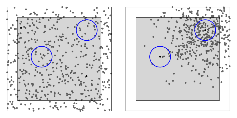
Figure 2: Two realizations of a Binomial point processes. Left shows a homogeneous point process and right shows an inhomogeneous point process.

Appendix C Definitions from Differential Geometry

C.1 A Discussion of Intrinsic and Extrinsic Validation

In general, model validation takes a model and quantifies the correctness of its output. There are two main classes of validation algorithms: extrinsic and intrinsic.

In extrinsic validation, the labels in data are known. In this case, the validation process compares a model’s output to the ground truth in order to quantify the model’s correctness. Extrinsic validation is generally the easiest and strongest method for validation, one particularly ubiquitous variant is precision and recall which has been studied in the context for manifolds in [24].

In intrinsic validation, the ground truth correct output of a model is not known. Thus, the validation process must use properties of only the model’s output in order to evaluate its correctness. A particularly notable example of intrinsic validation includes silhouette coefficients for clustering [29]. In practice, extrinsic validation typically accompanies supervised learning and intrinsic validation is often coupled with unsupervised learning. As the title alludes, this paper focuses on intrinsic validation.

C.2 A Review of Basic Definitions in Differential Geometry

We present fundamental definitions from differential geometry in the following section. For a survey, we suggest [7] and [23].

We begin with a formal definition of Riemannian metrics, which are crucial in the definition of a Riemannian manifold

Definition C.1 (Riemannian metric).

Let $(\mathbb{X},d)$ be a smooth manifold. We call $d$ a Riemannian metric if $d$ is a smooth covariant two-tensor field whose value $d_{x}$ at each $x\in\mathbb{X}$ is an inner product on the tangent space $T_{x}\mathbb{X}$.

On a manifold $\mathbb{X}$, we often study paths. A path between $x,y\in\mathbb{X}$ is a continuous map $\gamma:[0,1]\to\mathbb{X}$, where $\gamma(0)=x$ and $\gamma(1)=y$. A path $\gamma$ has length, which is defined as follows:

Definition C.2 (Length).

Let $(\mathbb{X},d)$ be a topological space and let $\gamma$ be a path in $(\mathbb{X},d)$. Let $\mathcal{P}$ be the set of all finite subsets $P=\{t_{i}\}$ of $[0,1]$ such that such that $0=t_{0}<t_{1}<...<t_{n}=1$. The length $L_{d}(\gamma)$ of $\gamma$ is:

$$L_{d}(\gamma):=\sup_{P\in\mathcal{P}}\sum_{i=1}^{n}{d(\gamma(t_{i}),\gamma(t_{i-1}))}.$$

The shortest paths between elements in $\mathbb{X}$ are usually of particular interest, which are called geodesics.

Definition C.3 (Geodesic).

Let $(\mathbb{X},d)$ be a topological space, let $x,y\in\mathbb{X}$, and let $\Gamma$ be the set of all paths in $(\mathbb{X},d)$ from $x$ to $y$. A geodesic $\gamma^{*}$ from $x$ to $y$ is a path with shortest length:

$$\gamma^{*}=\inf_{\gamma\in\Gamma}L_{d}(\gamma)$$

Let $U\subseteq\mathbb{X}$ be an open subset of $\mathbb{X}$, and let $\phi:U\to\mathbb{R}^{n}$ be a coordinate chart of $\mathbb{X}$ (that is, $\phi$ is a homeomorphism). We say that $\phi$ is smooth if for every $u\in U$, every component function of $\phi$ has continuous partial derivatives of every order. Let $U,V\subseteq\mathbb{X}$ be open subsets of $\mathbb{X}$ and examine two coordinate charts $\phi:U\to\mathbb{R}^{n}$ and $\psi:V\to\mathbb{R}^{n}$. We call $\phi,\psi$ smoothly compatible if both $\phi\circ\psi^{-1}$ and $\psi\circ\phi^{-1}$ are smooth when defined on $\phi(U\cap V)$ and $\psi(U\cap V$) respectively. An atlas of $\mathbb{X}$ is a set of coordinate charts whose domains cover $\mathbb{X}$, and an atlas is a smooth atlas if any two charts in the atlas are smoothly compatible. A smooth structure is a smooth atlas not properly contained in another smooth atlas. Finally, a smooth manifold is a manifold $\mathbb{X}$ equipped with a smooth structure.

Let $x\in\mathbb{X}$ and let $U$ be an open neighborhood of $x$. Let $C^{\infty}(V,\mathbb{R})$ be the set of all smooth mappings $f:U\to\mathbb{R}$. Let $f,g\in C^{\infty}(V,\mathbb{R})$. A tangent vector $T_{x}$ on $\mathbb{X}$ at $x$ is a linear map $T_{x}:C^{\infty}(V,\mathbb{R})\to\mathbb{R}$ satisfying the Leibniz law of products:

$$T_{x}(f\cdot g)=f(x)T_{x}(g)+g(x)T_{x}(f).$$

The tangent space on $T_{x}\mathbb{X}$ on $\mathbb{X}$ at $x$ is the set of all tangent vectors on $\mathbb{X}$ at $x$.

C.3 A Review of Tensor Products and the Volume Form

We begin with a condensed review of tensors, and describe one of their most important constructions in differential geometry: the volume form. For a more detailed description, we refer readers to [23]. We begin with alternating tensors and wedge products, and then proceed to the volume form itself.

Definition C.4 (Alternating Tensor).

Let $V$ be a finite-dimensional vector space, and let $F$ be a covariant $k$-tensor on $V$. We call $F$ an alternating tensor if the interchanging of two arguments causes $F$ to change sign:

$$F(v_{1},...,v_{i},...,v_{j},...,v_{k})=-F(v_{1},...,v_{j},...,v_{i},...,v_{k})$$

If $F$ is an alternating $k$-tensor, then it follows that for an arbitrary permutation of arguments $\sigma$,

$$F(v_{\sigma(1)},...,v_{\sigma(k)})=\text{sgn }\sigma F(v_{1},...,v_{k}).$$

Where sgn $\sigma$ is the sign of $\sigma$, giving $+1$ if $\sigma$ is an even permutation and $-1$ if $\sigma$ is odd. Similarly, the alternation of $F$ is given as follows:

Definition C.5 (Alternation).

Let $F$ be a covariant $k$-tensor. Let $S_{k}$ be the set of permutations of $F$. The alternation Alt $F$ of $F$ is given by the expression:

$$\text{Alt $F$}(v_{1},...v_{k})=\frac{1}{k!}\sum_{\sigma\in S_{k}}(\text{sgn }\sigma)F(v_{\sigma(1)},...,v_{\sigma(k)})$$

It is easy to check that Alt $F=F$ iff $F$ is alternating. Using the Alt operation, we define the wedge product of tensors:

Definition C.6 (Wedge Product).

Let $V$ be a finite-dimensional vector space. Let $F$ be an alternating covariant $k$-tensor on $V$, and let $G$ be an alternating covariant $l$-tensor on $V$. Then, their wedge product is defined by:

$$F\wedge G=\frac{(k+l)!}{k!l!}\text{Alt}(F\otimes G)$$

Where $F\otimes G$ is the usual tensor product.

Now, in order to understand the volume form rigorously, we present its definition below. Many definitions give the same property as the one below, along with two equivalent expressions. For simplicity we provide only the first property given in most definitions.

Definition C.7 (Volume Form).

Let $(\mathbb{X},g)$ be an oriented Riemannian manifold (with or without boundary). Let $(\varepsilon_{1},...,\varepsilon_{n})$ be a local oriented orthonormal coframe for $T^{*}\mathbb{X}$, the cotangent bundle of $\mathbb{X}$. The volume form $dV_{g}$, or $dV$ as a shorthand, is the unique $n$-form on $\mathbb{X}$ such that $dV_{g}=\varepsilon_{1}\wedge...\wedge\varepsilon_{n}$.

By design, if we have a continuous function $f:\mathbb{X}\to\mathbb{R}$ on a compact orientable Riemannian manifold (with or without boundary), then $f\cdot dV_{g}$ is a compactly supported $n$-frame, and taking an integral $\int_{\mathbb{X}}f\cdot dV_{g}$ is well defined. Moreover, if $\mathbb{X}$ is compact, the volume of $\mathbb{X}$ is defined canonically:

$$\text{Vol}(\mathbb{X})=\int_{\mathbb{X}}dV_{g}.$$

C.4 The Gauss-Codazzi Equations for Hypersurfaces

As with basic tensor operations, this article assumes a some working knowledge of concepts of curvature in differential geometry. For a detailed review of Riemannian, Ricci, Scalar, and Mean curvatures, as well as the second fundamental form, we again refer readers to Lee [23].

In the results for hypersurfaces, we use the second fundamental form and the length of the second fundamental form:

Definition C.8 (Second Fundamental Form).

Let $M$ be an $n$-dimensional hypersurface in of a Riemannian manifold $M^{\prime}$, and let $D$ and $D^{\prime}$ be their covariant derivatives. Then, for $m\in M$ and $u,v\in T_{m}M$ the second fundamental form $h$ of $M$ is given by:

$$h(u,v):=\left(D^{\prime}_{U}V-D_{u}V\right)_{m}^{\prime}$$

where $U,V$ are vector fields tangent to $M$ at any point of $M$, defined in a neighborhood of $m^{\prime}$ in $M^{\prime}$, and with respective values $u$ and $v$ at $m$.

Definition C.9 (Length of Second Fundamental Form).

Let $h$ be the second fundamental form at a point $p\in\mathbb{X}$, a Riemannian manifold. The squared length $||h||^{2}$ of $h$ is given by:

$$||h||^{2}=\sum_{i,j=1}^{n}h(E_{i},E_{j})^{2}$$

Where $E_{1},...,E_{n}$ is a local orthonormal frame of tangent vector fields over $\mathbb{X}$.

C.5 Hypersurfaces and their First Laplacian Eigenvalue

Naturally, after showing that the aggregated manifold density function can be scaled as a function of $\lambda_{1}$ in high dimensions, one wonders how to actually compute $\lambda_{1}$. The following lays out the bulk of known results for $\lambda_{1}$ with respect to a number of different manifolds.

Theorem C.1 (Conformal Clifford Torus).

If $M$ is a conformal Clifford torus, Then

$$\lambda_{1}*vol(M)\leq 4*\pi^{2}$$

Theorem C.2 (Veronese Surface).

If $M$ is a conformal Veronese surface, then we have

$$\lambda_{1}*\text{vol}(M)\leq 12*\pi,$$

with equality holding if and only if $M$ admits an order 1 isometric embedding.

Theorem C.3 (Submanifolds of Hyperspheres).

Let $M$ be an $n$-dimensional compact submanifold of a hypersphere $S^{m}(r)$ of radius $r$ in $\mathbb{R}^{m+1}$. Then $\lambda_{1}\leq n$, with equality holding iff $M$ is of order 1.

Theorem C.4 (Projective Plane).

Let $M$ be a compact, $n$-dimensional, minimal submanifold of $\mathbb{R}P^{m}$, where $\mathbb{R}P^{m}$ is of constant sectional curvature $1$. Then it follows that $\lambda_{1}\leq 2(n+1)$, with equality holding iff $M$ is a totally geodesic $\mathbb{R}P^{n}$ in $\mathbb{R}P^{m}$.

Theorem C.5 (Complex Projective Plane).

Let $M$ be an $n$-dimensional $(n\geq 2)$, compact, minimal submanifold of $\mathbb{C}P^{m}$, where $\mathbb{C}P^{m}$ is of constant holomorphic sectional curvature 4. Then we have $\lambda_{1}\leq 2(n+2)$

with equality holding iff $n$ is even, $M$ is a $\mathbb{C}P^{\frac{n}{2}}$, and $M$ is a complex totally geodesic submanifold of $\mathbb{C}P^{m}$.

Theorem C.6 (Quaternion Projective Plane).

Let $M$ be a compact, $n$-dimensional $(n\geq 4)$, minimal submanifold of $\mathbb{Q}P^{m}$, where $\mathbb{Q}P^{m}$ is of constant quaternion sectional curvature 4. Then we have $\lambda_{1}\leq 2(n+4)$, with equality holding iff $n$ is a multiple of $4$, $M$ is $\mathbb{Q}P^{\frac{n}{4}}$, and $M$ is embedded in $\mathbb{Q}P^{m}$ as a totally geodesic quaternionic submanifold.

Theorem C.7 (Cayley Plane).

Let $M$ be a compact, $n$-dimensional, minimal submanifold of the Cayley Plane $OP^{2}$, where $OP^{2}$ is of maximal sectional curvature 4. Then we have $\lambda_{1}\leq 4n$.

Theorem C.8 (CR Submanifolds of $\mathbb{C}P^{n}$).

Let $M$ be a compact, $n$-dimensional, minimal, $CR$-submanifold of $\mathbb{C}P^{m}$. Then we have $\lambda_{1}\leq 2(n^{2}+n+2a)/n$, where $a$ is the complex dimension of the holomorphic distribution.

Theorem C.9 (CR Submanifolds of $QP^{m}$).

Let $M$ be a compact, $n$-dimensional, minimal CR-submanifold of $QP^{m}$. Then we have $\lambda_{1}\leq 2(n^{2}+n+12a)/n$ where $a$ is the quaternionic dimension of the quaternion distribution.

Appendix D Experimental Results

We present our experimental findings, comparing the manifold score of samples on popular manifolds. Our anonymized code is accessible at the following url for reproducibility:

https://anonymous.4open.science/r/intrinsic-manifold-validation/

D.1 Results on Flat Manifolds

As an initial verification, we test the framework on an embedding of the flat $2$-torus, where we expect the manifold score to be nearly perfect (close to one) for a uniform sample. We compare this against a stratification on the flat torus, sampled uniformly in the form of a “cross,” $\{(x,y):x=\frac{1}{2}\text{ or }y=\frac{1}{2}\}\subset[0,1)\times[0,1)$. We also consider a sample of the “cross”-stratification with noise, where ten percent of the sample’s points are uniformly sampled from the domain graph of the flat torus. Table 1 gives the average aggregated manifold score across ten trials on the flat $2$-torus for these three samples. As anticipated, the manifold score is nearly perfect for the uniform sample, worse for the stratification with noise, and even worse for the pure stratification.

Table 1: Manifold Score on the Flat Torus

Sample Size	Uniform Sample	Strat. with Noise	Stratification
100	$0.9840\pm 0.0056$	$0.8807\pm 0.0158$	$0.6768\pm 0.0490$
200	$0.9921\pm 0.0023$	$0.8769\pm 0.0178$	$0.6410\pm 0.0339$
500	$0.9962\pm 0.0010$	$0.8763\pm 0.0071$	$0.6537\pm 0.0210$
1000	$0.9980\pm 0.0009$	$0.8728\pm 0.0074$	$0.6545\pm 0.0241$

D.2 Surfaces with Curvature

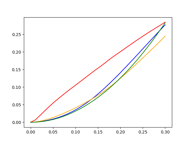
Figure 3: From left to right: (1) uniform sample vs. (2) minor noise vs (3) stratification on the Klein bottle with $|X|=2000$. The right plot compares the normalized manifold density functions of each, with (1) in blue, (2) in orange, (3) red, and the theoretical manifold density function in green.

We compare the manifold score of stratifications vs. uniform samples on both the sphere and the Klein bottle. We generate a distance matrix using ISOMAP with six neighbors, conducting ten trials for each experiment. For the sphere, we scale according to the approximation following Corollary 3.1 setting $A\approx r^{2}$. A uniform sampling and “cross”-stratification were considered, and the results are presented in Table 2. We note the impact of proper scaling on the manifold score. For the Klein bottle, we use no scaling since the Euler characteristic is zero. We again consider a uniform sample and “cross”-stratification, as well as a noisy sample obtained by sampling with probabilities defined by a normalized sine wave across the surface. As demonstrated by Table 3, the manifold score is effective in evaluating the sample’s representation of the Klein bottle.

For both surfaces, the manifold score converges to one (a perfect score) as the uniform sample size increases, which is explained by Theorem 3.1. However, this convergence is slower than for the flat torus, which we attribute to the introduction of a neighbors graph rather than using true geodesics, as well as the heuristic nature of the definition of the aggregated manifold density function for general two-manifolds.

Table 2: Results on the Sphere

Sample Size	Scaled Unif.	Unscaled Unif.	Stratification
100	$0.9415\pm 0.0169$	$0.7770\pm 0.0147$	$0.6116\pm 0.1801$
500	$0.9443\pm 0.0083$	$0.7834\pm 0.0256$	$0.6101\pm 0.1842$
1000	$0.9583\pm 0.0151$	$0.7840\pm 0.0123$	$0.6597\pm 0.2110$
2000	$0.9730\pm 0.0096$	$0.7963\pm 0.0110$	$0.6310\pm 0.2382$

Table 3: Results on the Klein Bottle

Sample Size	Uniform	Minor Noise	Stratification
200	$0.8834\pm 0.0571$	$0.8114\pm 0.0760$	$0.3578\pm 0.0926$
500	$0.9109\pm 0.0334$	$0.8942\pm 0.0386$	$0.4048\pm 0.1521$
1000	$0.9430\pm 0.0105$	$0.8417\pm 0.1286$	$0.5054\pm 0.0558$
2000	$0.9529\pm 0.0081$	$0.8735\pm 0.0520$	$0.3075\pm 0.0630$

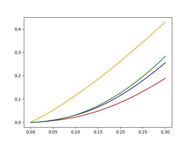
Figure 4: From left to right: (1) uniform sample vs. (2) a stratification on the sphere, with $|X|=1000$. The right plot compares the manifold density functions of each, with (1) scaled in blue, (1) unscaled in red, (2) in orange, and the theoretical manifold density function in green.

Next, we develop a more in depth discussion of the manifold score on the Klein bottle, and implement the comparison of manifold learning algorithms shown in Figure 1 in Section 2. This anecdote provides a sense for both the intended positive behavior and the shortcomings of our use of the manifold density function, which appear inherent to intrinsic validation in general. Namely, we lift a parameterization of the Klein bottle in $\mathbb{R}^{3}$ to ten dimensions by assigning values from the interval $[0,2\pi]$ uniformly at random to each of the other seven coordinates. In total, this point cloud representation lying on an ambient Klein bottle in 3D has 1000 points. We then attempt to re-learn the 3D parameterization of the Klein bottle; computing embeddings in $\mathbb{R}^{3}$ of the point cloud in $\mathbb{R}^{1}0$ using PCA, ISOMAP, t-SNE, LLE, and spectral embedding, each with $n_{components}=3$ and $n_{neighbors}=6$. To the naked eye, PCA appears to perform the best, simply by dropping the other seven dimensions, and ISOMAP also appears to perform well, albeit a bit worse. In actuality, ISOMAP assigns much greater density to the handle region of the Klein bottle in this example, and achieves a somewhat unfavorable score. This provides an adversarial example where t-SNE outperforms ISOMAP, despite the visual preferability of the latter. The results when evaluating the manifold score on each algorithm are summarized in the following table, where we report the manifold score on the manifold density function restricted to radius $r=0.3$:

Table 4: Differing Manifold Scores from the Klein Bottle

PCA	ISOMAP	t-SNE	LLE	Spectral Embedding
$0.9557$	$0.7179$	$0.9154$	$0.3988$	$0.6881$

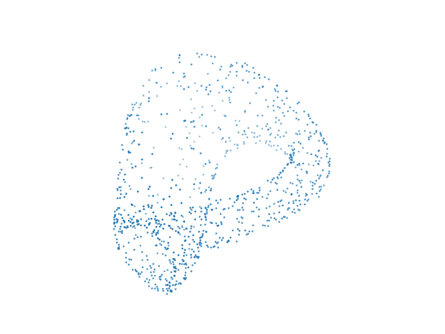
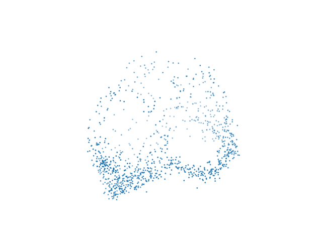
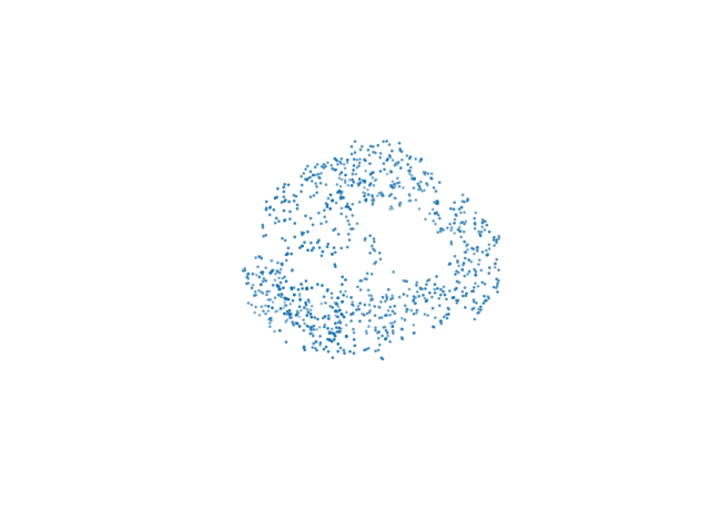
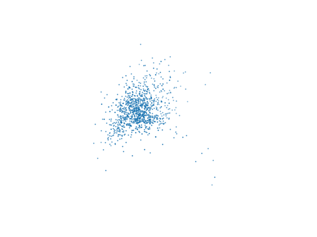
Figure 5: Embeddings of the Klein bottle in $\mathbb{R}^{3}$ after being projected from $\mathbb{R}^{10}$ from left to right: PCA, ISOMAP, and t-SNE (top) locally linear embedding and spectral embedding (bottom).

Upon visual inspection, the apparent best performing algorithm in this example (PCA) is indeed detected as performing well, while the worse performing algorithms are generally detected as such. However, the manifold score is not able to distinguish between ISOMAP and t-SNE in the example, despite visually ISOMAP appearing to better uncover the manifold. This illuminates a shortcoming of the manifold score; which is a consequence of working in the unsupervised setting. That is, without knowledge of the ground truth manifold which we are attempting to uncover, there is no way of distinguishing between a uniform sample of something more distantly resembling a desired manifold, and a nonuniform sample closely resembling a desired manifold.

D.3 Hypersurfaces

In higher dimensions, we use the results of Section 3.4 to examine uniform samples on hyperspheres in six, eight, ten, and fifteen dimensions. We demonstrate the manifold score of a uniform sample pre and post scaling, and the analogous stratification to the one in Figure 4 of two $d/2$-dimensional hyperspheres (scaled equivalently). For each experiment, we work with samples of size 1000 over ten trials. In higher dimensions the volume of Euclidean balls decreases, making the manifold score increasingly sensitive; yet we are still able to delineate between uniform samples and stratifications with the needed specificity.

Table 5: Results on Hyperspheres of Differing Dimension

Dimension	Scaled Unif.	Unscaled Unif.	Stratification
6	$0.9747\pm 0.0022$	$0.9143\pm 0.0056$	$0.8033\pm 0.0023$
8	$0.9803\pm 0.0010$	$0.9256\pm 0.0034$	$0.8782\pm 0.0043$
10	$0.9895\pm 0.0004$	$0.9458\pm 0.0019$	$0.9239\pm 0.0029$
15	$0.9968\pm 0.0003$	$0.9692\pm 0.0033$	$0.9697\pm 0.0014$

In what follows, we outline the resulting manifold density functions for hyperspheres, tabulated in their corresponding dimension. We provide a more complete experiment here, including edge cases in lower and higher dimensions than the cases included in experiments in the main body. Interestingly, only upon reaching five dimensions does scaling the manifold density function for hypersurfaces become beneficial, which we attribute to the fact that our scaling is indeed approximate; if possible to work with two-manifolds the exact scaling afforded by the Gauss-Bonnet theorem is preferable. In very high dimensions, as expected, it becomes increasingly subtle (but still possible outside of the range of error) to distinguish between uniform samples nonuniform samples such as the stratification. Once again, we employ a stratification of two $d/2$ hyperspheres sampled on the surface of the $d$-dimensional hypersphere.

Table 6: Results on Hyperspheres of Differing Dimension

Dimension	Post Scaling	Pre Scaling	Stratification
3	$0.6801\pm 0.0074$	$0.7791\pm 0.0093$	$0.6251\pm 0.0016$
4	$0.9143\pm 0.0043$	$0.9785\pm 0.0046$	$0.8291\pm 0.0899$
5	$0.9823\pm 0.0006$	$0.9207\pm 0.0049$	$0.7936\pm 0.0805$
20	$0.9983\pm 0.00002$	$0.9732\pm 0.0003$	$0.9842\pm 0.0015$
50	$0.9997\pm 0.000001$	$0.9736\pm 0.00012$	$0.9982\pm 0.000039$
100	$0.9999\pm 0.0000003$	$0.9735\pm 0.00013$	$0.9995\pm 0.0000085$

References

- [1] H. Amann, J. Escher, and G. Brookfield, Analysis III, Springer, 2009.
- [2] A. J. Baddeley, J. Møller, and R. Waagepetersen, Non-and semi-parametric estimation of interaction in inhomogeneous point patterns, Statistica Neerlandica, 54 (2000), pp. 329–350.
- [3] M. Belkin and P. Niyogi, Laplacian eigenmaps for dimensionality reduction and data representation, Neural Computation, 15 (2003), pp. 1373–1396.
- [4] C. M. Bishop, M. Svensén, and C. K. I. Williams, Gtm: The generative topographic mapping, Neural Computation, 10 (1998), pp. 215–234.
- [5] G. Carlsson, T. Ishkhanov, V. De Silva, and A. Zomorodian, On the local behavior of spaces of natural images, International Journal of Computer Vision, 76 (2008), pp. 1–12.
- [6] I. Chavel, Eigenvalues in Riemannian Geometry, Academic Press, 1984.
- [7] B.-Y. Chen, Total Mean Curvature and Submanifolds of Finite Type, 05 1984.
- [8] S. N. Chiu, D. Stoyan, W. S. Kendall, and J. Mecke, Stochastic geometry and its applications, John Wiley & Sons, 2013.
- [9] N. Cressie, Statistics for spatial data, John Wiley & Sons, 2015.
- [10] D. J. Daley, D. Vere-Jones, et al., An introduction to the theory of point processes: volume I: elementary theory and methods, Springer, 2003.
- [11] A. Dirafzoon, A. Bozkurt, and E. Lobaton, Geometric learning and topological inference with biobotic networks, IEEE Transactions on Signal and Information Processing over Networks, 3 (2016), pp. 200–215.
- [12] P. M. Dixon, Ripley’s K Function, John Wiley & Sons, Ltd, 2014.
- [13] D. Donoho and C. Grimes, Hessian eigenmaps: Locally linear embedding techniques for high-dimensional data. proc. national academy of science (pnas), 100, 5591-5596, Proceedings of the National Academy of Sciences of the United States of America, 100 (2003), pp. 5591–6.
- [14] C. Fefferman, S. Mitter, and H. Narayanan, Testing the manifold hypothesis, Journal of the American Mathematical Society, 29 (2016), pp. 983–1049.
- [15] S. Gallot, D. Hulin, and J. Lafontaine, Riemannian Geometry, Universitext, Springer Berlin Heidelberg, 2004.
- [16] L. Haizhong, Hypersurfaces with constant scalar curvature in space forms, Mathematische Annalen, 305 (1996), pp. 665–672.
- [17] F. Hensel, M. Moor, and B. Rieck, A survey of topological machine learning methods, Frontiers in Artificial Intelligence, 4 (2021).
- [18] A. Hohl and P. Chen, Spatiotemporal simulation: local ripley’s k function parameterizes adaptive kernel density estimation, in Proceedings of the 2nd ACM SIGSPATIAL International Workshop on GeoSpatial Simulation, 2019, pp. 16–23.
- [19] X. Huo and A. Smith, A survey of manifold-based learning methods, Recent Advances in Data Mining of Enterprise Data, (2008).
- [20] M. Jin, W. Zeng, N. Ding, and X. Gu, Computing Fenchel-Nielsen coordinates in Teichmuller shape space, in 2009 IEEE International Conference on Shape Modeling and Applications, IEEE, 2009, pp. 193–200.
- [21] A. Karr, Point processes and their statistical inference, Routledge, 2017.
- [22] T. J. Lawrence, Point pattern analysis on a sphere, Master’s thesis, Master’s thesis, The University of Western Australia, 2018.
- [23] J. Lee, Introduction to Riemannian Manifolds, Graduate Texts in Mathematics, Springer International Publishing, 2019.
- [24] M. Madhyastha, G. Li, V. Strnadová-Neeley, J. Browne, J. T. Vogelstein, R. Burns, and C. E. Priebe, Geodesic forests, in Proceedings of the 26th ACM SIGKDD International Conference on Knowledge Discovery & Data Mining, KDD ’20, New York, NY, USA, 2020, Association for Computing Machinery, p. 513–523.
- [25] J. Møller and E. Rubak, Functional summary statistics for point processes on the sphere with an application to determinantal point processes, Spatial Statistics, 18 (2016), pp. 4–23.
- [26] H. Narayanan and S. Mitter, Sample complexity of testing the manifold hypothesis, in Advances in Neural Information Processing Systems, J. Lafferty, C. Williams, J. Shawe-Taylor, R. Zemel, and A. Culotta, eds., vol. 23, Curran Associates, Inc., 2010.
- [27] B. D. Ripley, Locally finite random sets: Foundations for point process theory, The Annals of Probability, (1976), pp. 983–994.
- [28] B. D. Ripley, Statistical inference for spatial processes, Cambridge university press, 1988.
- [29] P. J. Rousseeuw, Silhouettes: A graphical aid to the interpretation and validation of cluster analysis, Journal of Computational and Applied Mathematics, 20 (1987), pp. 53–65.
- [30] S. T. Roweis and L. K. Saul, Nonlinear dimensionality reduction by locally linear embedding, Science, 290 (2000), pp. 2323–2326.
- [31] L. A. Santaló, Integral Geometry and Geometric Probability Addison Wesley, Cambridge University Press, 2nd ed., 2004.
- [32] J. Sporring, R. Waagepetersen, and S. Sommer, Generalizations of ripley’s k-function with application to space curves, in Information Processing in Medical Imaging: 26th International Conference, IPMI 2019, Hong Kong, China, June 2–7, 2019, Proceedings 26, Springer, 2019, pp. 731–742.
- [33] K. Streib and J. W. Davis, Using ripley’s k-function to improve graph-based clustering techniques, in CVPR 2011, IEEE, 2011, pp. 2305–2312.
- [34] W. Tang, W. Feng, and M. Jia, Massively parallel spatial point pattern analysis: Ripley’s k function accelerated using graphics processing units, International Journal of Geographical Information Science, 29 (2015), pp. 412–439.
- [35] J. B. Tenenbaum, V. de Silva, and J. C. Langford, A global geometric framework for nonlinear dimensionality reduction, Science, 290 (2000), pp. 2319–2323.
- [36] J. von Rohrscheidt and B. Rieck, Topological singularity detection at multiple scales, 2023.
- [37] S. Ward, Analysis of Spatial Point Patterns on Surfaces, PhD thesis, Imperial College London, 2021.
- [38] S. Ward, H. Battey, and E. Cohen, Nonparametric estimation of the intensity function of a spatial point process on a riemannian manifold, Biometrika, (2023), p. asad012.
- [39] N. Zheng and J. Xue, Manifold Learning, Springer London, London, 2009, pp. 87–119.
- [40] , Statistical Learning and Pattern Analysis for Image and Video Processing, Springer Science & Business Media, 2009.