Guided Quantum Compression for Higgs Identification

Abstract

Quantum machine learning provides a fundamentally novel and promising approach to analyzing data. However, many data sets are too complex for currently available quantum computers. Consequently, quantum machine learning applications conventionally resort to dimensionality reduction algorithms, e.g., auto-encoders, before passing data through the quantum models. We show that using a classical auto-encoder as an independent preprocessing step can significantly decrease the classification performance of a quantum machine learning algorithm. To ameliorate this issue, we design an architecture that unifies the preprocessing and quantum classification algorithms into a single trainable model: the guided quantum compression model. The utility of this model is demonstrated by using it to identify the Higgs boson in proton-proton collisions at the LHC, where the conventional approach proves ineffective. Conversely, the guided quantum compression model excels at solving this classification problem, achieving a good accuracy. Additionally, the model developed herein shows better performance compared to the classical benchmark when using only low-level kinematic features.

I Introduction

Machine Learning (ML) has been established as an invaluable tool for analysing data, assisting many physics analyses and discoveries at the Large Hadron Collider (LHC) Plehn et al. (2022); Guest et al. (2018); Karagiorgi et al. (2021); Belis et al. (2024). Meanwhile, quantum computing is a fundamentally different paradigm for information processing, that is known to provide computational speed-ups over classical methods for a large class of problems Grover (1996); Shor (1997); Harrow et al. (2009); Arute et al. (2019); Zhong et al. (2020); Madsen et al. (2022); Babbush et al. (2023). Furthermore, Quantum Machine Learning (QML) has the potential to enhance classical ML methods Biamonte et al. (2017); Schuld and Petruccione (2018); Benedetti et al. (2019); Havlíček et al. (2019); Schuld and Killoran (2019); M. Schuld et al. (2020), and has promise to yield advantages in certain learning tasks Rebentrost et al. (2014); Liu et al. (2021); Huang et al. (2021, 2022); Muser et al. (2023); Pirnay et al. (2023); Gyurik and Dunjko (2022). Recent studies have highlighted guarantees regarding the expressivity, generalisation power, and trainability of quantum models Pérez-Salinas et al. (2020); Schuld (2021); Goto et al. (2021); Abbas et al. (2021); Caro et al. (2022); Jerbi et al. (2023). The efficacy of applying QML models to High Energy Physics (HEP) data analysis has been exemplified in studies for classification Wu et al. (2021a, b); Terashi et al. (2021); Belis et al. (2021); Blance and Spannowsky (2020); Gianelle et al. (2022), reconstruction de Lejarza et al. (2022); Tüysüz et al. (2020); Magano et al. (2022), anomaly detection Ngairangbam et al. (2022); Schuhmacher et al. (2023); Alvi et al. (2023); Woźniak et al. (2023), and Monte Carlo integration de Lejarza et al. (2024); Agliardi et al. (2022). A recent summary of advancements in this field can be found in Ref. dim (2023).

However, for most realistic applications, the dimensionality of the dataset is usually too large to be directly processed by commonly available quantum computers. Consequently, dimensionality reduction techniques are typically employed and treated as a preprocessing step before the data is loaded into the QML algorithm. Previous studies use manual feature selection, informed by prior knowledge about the given problem Terashi et al. (2021); Belis et al. (2021), feature extraction techniques, such as the popular Principal Component Analysis (PCA) Wu et al. (2021a, b); Schuhmacher et al. (2023), or more recently, dimensionality reduction using deep learning models, e.g., simple auto-encoders Belis et al. (2021); Woźniak et al. (2023); Ballard (1987). Within the aforementioned literature, all of these approaches are shown to work for specific datasets; however, there is no guarantee that the lower-dimensional representation of the dataset is able to preserve the original class structure. Concretely, crucial information required in discriminating between the classes can be lost in the dimensionality reduction procedure, rendering the classification task harder or even impossible.

To address this challenge, we design a model architecture that generates lower dimensional representations optimised for quantum model classification performance. We call this approach guided quantum compression. Here, dimensionality reduction is not treated as a separate preprocessing step, pervasive in the majority of realistic QML applications; instead, guided quantum compression simultaneously accomplishes the dimensionality reduction and classification tasks with a single model. This way, the performance of the QML is not limited by the arbitrary choice of the reduction method.

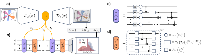
Figure 1: The GQC network. The architecture of the GQC network is shown in a) and b). The auto-encoder receives data from simulated LHC proton-proton collisions and produces a lower dimensional representation $z\in\mathbb{R}^{\ell}$ via the encoder network $\mathcal{E_{\omega}}$, where $\ell$ is called the latent space dimension. The decoder network $\mathcal{D_{\rho}}$, receives $z$ and aims to reconstruct the original data $x$. The distinct segments $z_{1},\dots,\,z_{i},\dots,\,z_{d}$ of the latent space vector $z$ are encoded sequentially in the quantum circuit by using the feature map $U(\cdot)$; the dimension of $z_{i}$ is equal to the number of qubits $n$ in the circuit. The trainable gates $G(\cdot)$ are placed between the quantum encoding gates $U(\cdot)$. The output of the decoder network and quantum model are used to minimize different parts of the total loss function $\mathcal{L}$ from Eq. 7. c) The data encoding circuit $U(\cdot)$ Havlíček et al. (2019) described in Sec. II.2. d) The variational ansatz $G(\cdot)$. The indices $j=1,\dots,\,n$ enumerate the elements of $z_{i}$. Moreover, the indices $l=1,\dots,\,2nr$ pertain to the trainable parameter of the corresponding $k$-th parametrised circuit block $G(\vartheta_{k})$, where $r$ are the repetitions of the trainable ansatz.

We show that for a realistic and complex classification task, i.e., identifying the Higgs boson in the $t\bar{t}H(b\bar{b})$ semileptonic channel for simulated proton collision data at the LHC, the conventional reduction methods fail: independently compressing the dataset before training the QML model leads to poor classification performance. In contrast, the guided quantum compression method is able to solve the classification problem, reaching competitive accuracy with state-of-the-art classical methods Donega et al. (2021). Furthermore, we observe an improved performance of the quantum compression algorithm with respect to the classical benchmark when only features that describe the particle kinematics are used. Thus, suggesting that for an improved performance of quantum learners on particle physics data, the employed features should be representative of the quantum process that generated the data Collaboration (2019); Kübler et al. (2021), e.g., the particle momenta, rather than classically processed high level information Schuhmacher et al. (2023); Woźniak et al. (2023).

II Models

The guided quantum compression network shown in Fig. 1 is comprised of an auto-encoder (Fig. 1a) and a variational quantum circuit (Fig. 1b) that are coupled. In the following, we describe these two elements and how they are simultaneously trained.

II.1 The Auto-encoder

The auto-encoder (AE) is a machine learning model that had been used for decades across the historical landscape of neural networks LeCun (1987); Ballard (1987); Hinton and Zemel (1993). The most commonly used type of AE consists of two feed-forward neural networks: the encoder $\mathcal{E}_{\omega}$ and the decoder $\mathcal{D}_{\rho}$. The encoder $\mathcal{E}_{\omega}$ maps the input feature space $x$ to a latent space $z$ of lower dimension $\ell$. Conversely, the goal of the decoder $\mathcal{D}_{\rho}$ is to reconstruct the input $x$ from $z$. A schematic of an AE neural network is shown in Fig. 1a. The objective of the AE training is to minimise the difference between the input data and the reconstructed data; this difference can be quantified by various functions. There exist many types of AEs, based on how this difference is quantified or on architectural extensions Kingma and Welling (2013); Deja et al. (2021); Joo et al. (2020); Pan et al. (2018). The Mean Squared Error (MSE) is the standard function used to quantify the difference between the input data $x$ and its reconstructed counterpart:

$$\mathcal{L}_{R}=\frac{1}{M}\sum^{M}_{m=1}\left[x_{m}-\mathcal{D}_{\rho}\circ\mathcal{E}_{\omega}(x_{m})\right]^{2},$$ (1)

where $\mathcal{D_{\rho}}$ is the decoder network with weights $\rho$, $\mathcal{E}_{\omega}$ is the encoder network with weights $\omega$, and $M$ is the size of the training data set. The conventional AE learns as any other feed-forward neural network, with one subtlety: the reconstruction loss is not only propagated through the decoder network, but through the encoder as well. Therefore, the latent space and the reconstructed data evolve simultaneously as the AE model is learning.

II.2 The Variational Quantum Circuit

The Variational Quantum Circuit (VQC) Benedetti et al. (2019); Mitarai et al. (2018) is a QML model based on parametrized quantum circuits that are trained variationally to undertake tasks such as classification Blance and Spannowsky (2020); Belis et al. (2021); Wu et al. (2021b); Terashi et al. (2021), regression Pérez-Salinas et al. (2021), and generative modelling Chang et al. (2021); Kiss et al. (2022); Delgado and Hamilton (2022); Bravo-Prieto et al. (2022). The classifier output, in the VQC implementation, is the expectation of an observable $\mathcal{M}$. This expectation is interpreted as the likelihood of the input sample to belong in a certain data class, e.g., the sample contains a Higgs boson or not, and is extracted from the quantum computer via doing measurements. Specifically, the model output $f_{\vartheta}(z)$, for a given input data vector $z$ and gate parameters $\vartheta$, is defined as

$$f_{\vartheta}(z)=\Braket{0}{\mathcal{U}_{\vartheta}^{\dagger}(z)\mathcal{M}\,\mathcal{U}_{\vartheta}\left(z\right)}{0}=\Braket{\mathcal{M}_{\vartheta}(z)},$$ (2)

where $\mathcal{U}_{\vartheta}(z)$ is the whole quantum circuit of the model, $\mathcal{M}$ is the observable whose expectation value we measure, and $\ket{0}=\ket{0}^{\otimes n}$ the initial $n$ qubit state. Furthermore, the label predicted by the VQC, $\hat{y}\in\{0,1\}$, is given by

$$\hat{y}=\frac{\text{sign}\left[\braket{\mathcal{M}_{\vartheta}(z)}\right]+1}{2},$$ (3)

where one can assume that $\braket{\mathcal{M}_{\vartheta}(z)}\in[-1,1]$ without any loss of generality.

We design a VQC architecture as shown in Fig. 1b. The input data vector $z$ is split into $d$ sub-vectors $z=(z_{1},z_{2},\dots,z_{d})$, each $z_{i}$ being of dimensionality $n$. Furthermore, each sub-vector is encoded into the quantum circuit sequentially by using the feature map $U(\cdot)$; between each $U(\cdot)$ there is a set of trainable gates $G(\cdot)$. Hence, the whole quantum circuit of the model is

$$\mathcal{U}_{\vartheta}(z)=\prod_{k=1}^{d}G(\vartheta_{k})U(z_{k}).$$ (4)

The proposed architecture design is theoretically motivated by how the VQC model expressivity increases with the circuit depth Pérez-Salinas et al. (2020); Schuld et al. (2021). Furthermore, through our encoding strategy, we are able to tune the number of qubits and the number of gate operations in the VQC circuit. This way, we ensure $d=\ell/n$, where $d$ is the number of segments of the latent vector $z$ and $\ell$ is the dimensionality of the latent space produced by the auto-encoder.

Here, we set the observable $\mathcal{M}\equiv\sigma_{z}$, where $\sigma_{z}$ is the Pauli-Z operator acting on the first qubit. The data encoding $U(\cdot)$ used herein is the feature map from Ref. Havlíček et al. (2019). This consists of $R_{z}$ rotation gates, which encode one data feature per qubit, and nearest-neighbor entanglement between these qubits, as presented in Fig. 1c. The data encoding blocks include interactions between the features:

$$\phi(z_{i}^{(j)},z_{i}^{(j+1)})=\prod_{j=1}^{n}\left(\pi-z_{i}^{(j)}\right)\left(\pi-z_{i}^{(j+1)}\right),$$ (5)

where the quantities are as described in Fig. 1c and Fig. 1d. A single repetition of the variational ansatz applies $R_{Y}$ rotations on each qubit and nearest-neighbor entanglement via the CNOT (CX) gates, as in Fig. 1d.

We choose these general purpose data encoding and trainable circuits to highlight the effectiveness of the GQC network in solving classification tasks that conventional methods would struggle with. Hence, we do not focus on an extensive search for the quantum circuits that would yield the best classification performance; our results do not depend a specific choice of VQC architecture.

All classifiers in this work are trained to minimise the binary cross entropy loss function:

$$\mathcal{L}_{C}=-\frac{1}{M}\sum_{m=1}^{M}\left[y_{m}\log(\hat{y}_{m})+(1-y_{m})\log(1-\hat{y}_{m})\right],$$ (6)

where $M$ is the number of data points, e.g., in a batch, $y_{m}$ is the true label of the data point $m$, and $\hat{y}_{m}$ is its predicted label, as in Eq. 3.

III Training Paradigms

Three different training workflows are investigated. First, the so called classical approach, which serves as our baseline benchmark. Second, the 2Step method, which represents the usual way to perform dimensionality reduction when using QML for classifying complex data. Finally, the GQC paradigm developed in this work, which performs the dimensionality reduction and classification objectives at the same time.

Note, the three aforementioned strategies pertain to different computational requirements: it is less computationally intensive to train and robustly optimise the hyperparameters of a classical algorithm compared to a quantum one. Thus, for the hyperparameters of the classical network, we are able to find their optimal values. Conversely, this is not technically achievable for the quantum models presented in this work: the amount of compute time required is unfeasible. Furthermore, a vast amount of computational resources (cf. App. A) are required to find the best quantum hyperparameter combination, i.e., the best number of trainable ansatz repetitions, the best number of qubits, the best learning rate, and so on.

III.1 Classical

A feed-forward network is our classical benchmark. This network is trained to minimise the binary cross entropy loss, in Eq. 6, via stochastic gradient descent. In essence, the classical paradigm represents the most conventional way to address our classification task.

The hyperparameters of the feed-forward network, such as the learning rate, are optimized by doing a grid search. This is the only type of model and paradigm for which an exhaustive hyperparameter optimisation is feasible.

III.2 2Step

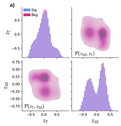
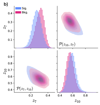
Figure 2: Latent representation. The one- and two-dimensional projections of the $t\bar{t}H(b\bar{b})$ dataset latent space $z\in\mathbb{R}^{\ell}$ generated by a) the 2Step training paradigm and b) GQC model. The probability distributions of the latent features $z_{7}$ and $z_{10}$ are shown in the histogram plots. The joint two-dimensional probability distributions $\mathcal{P}(z_{7},z_{10})$ are displayed in the density plots. Notice that the latent space separation of signal and background is better in the GQC algorithm; furthermore, the GQC latent distributions are more regularly shaped. The latent features $z_{7}$ and $z_{10}$ are arbitrarily chosen to show the structure of the latent vector $z$ in one or two dimensions. These joint distributions are symmetric: $\mathcal{P}(z_{7},z_{10})=\mathcal{P}(z_{10},z_{7}).$

In this paradigm, the dimensionality reduction algorithm, namely the AE from Sec. II.1, is trained independently from the classification algorithm from Sec. II.2. As the name suggests, the classification task is performed in two separate steps. First, the hyperparameters of the AE are optimised and the resulting architecture is trained with the goal of minimising the MSE loss between the input data and the output of the decoder. Secondly, the VQC is trained by using the latent space representation $z$ of each sample that the AE produces. This way, the VQC acts on a lower dimensional input and consequently its quantum circuit can be smaller. As mentioned in Sec. I, the dimensionality reduction allows us to employ a reasonable amount of resources in simulating quantum circuits in classical devices and in implementing our quantum models in currently available quantum computers. Hitherto, we outlined the most common way in which AEs are used for dimensionality reduction in the context of a classification task Wang et al. (2016); in the following, a paradigm which integrates the two steps is defined.

III.3 Guided Quantum Compression

Our strategy aims to address the problem of generating a low-dimensional representation that ensures the discrimination of the classes by the quantum model. The GQC network implements a trainable data encoding map $\mathcal{U}_{\vartheta}\left(\mathcal{E}_{\omega}(x)\right)$. The lower-dimensional representation learned by the encoder network is guided by the quantum classification algorithm.

The guidance is performed during the training of the GQC network by coupling the auto-encoder and VQC models through the following loss function:

$$\mathcal{L}=(1-\lambda)\mathcal{L}_{R}+\lambda\mathcal{L}_{C},$$ (7)

where $\mathcal{L}_{R}$ is the MSE loss as defined in Eq. 1, $\mathcal{L}_{C}$ is the loss of the VQC classifier defined in Eq. 6, and $\lambda\in(0,1)$ is the hyperparameter that tunes the coupling between the reconstruction and classification optimisation tasks.

The simultaneous learning of the two objectives improves the generalisation power of the classifier Le et al. (2018); Vafaeikia et al. (2020). This synergy arises from the regularisation imposed through Eq. 7 of the quantum classifier. Namely, the classifier performance is enhanced by the additional task of reconstructing data from the latent space Vafaeikia et al. (2020).

In our algorithm, we train the GQC network via stochastic gradient descent, using the Adam optimizer Kingma and Ba (2017). The gradients of the classical parts of the model are computed using backpropagation, while the quantum circuit gradients are computed via the adjoint differentiation method Jones and Gacon (2020), for efficient training of the model on classical processors used to simulate the quantum software. The proposed GQC architecture can also be trained on quantum hardware using the parameter-shift rule Schuld et al. (2019) instead of the adjoint differentiation method. The hyperparameters of the GQC network are tuned using a sequential grid search for each hyperparameter while keeping all the rest fixed. For more details please refer to App. A.

IV Results

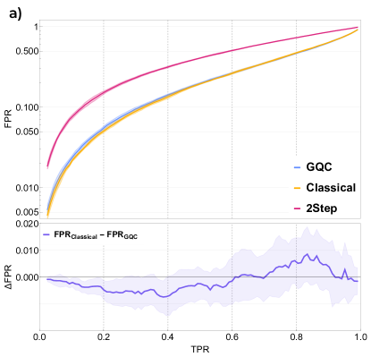
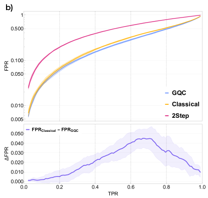
Figure 3: Receiver Operating Curves. The ROC curves of the models with a) the btag features and b) without the btag features included in the training data. The 2Step training procedure yields the worst performance. At the bottom panel of each plot the difference between the GQC ROC and the classical ROC is displayed. When the btag is absent from the dataset, the GQC model outperforms the classical benchmark in the TPR range of $0.4$ to $0.9$, as shown in the lower panel of b).

Model	AUC w/ b-tag	AUC w/o b-tag	FPR-1 w/ b-tag	FPR-1 w/o b-tag
GQC	$0.733\pm 0.003$	$\mathbf{0.720\pm 0.005}$	$2.134\pm 0.028$	$2.045\pm 0.049$
2Step	$0.561\pm 0.003$	$\mathbf{0.508\pm 0.002}$	$1.263\pm 0.004$	$1.368\pm 0.007$
Classical	$0.734\pm 0.002$	$\mathbf{0.699\pm 0.004}$	$2.107\pm 0.029$	$1.921\pm 0.035$

Table 1: Model Performances. The first two columns present the Area Under the Curve (AUC) values of the three training paradigms with and without the b-tag variable in the training data, respectively. The last two columns show the inverse FPR at $\mathrm{TPR}=0.8$.

The three training paradigms described in Sec. III are benchmarked using a simulated $t\bar{t}H(b\bar{b})$ data set collaboration (2019); Collaboration (2022). This is a classification data set with two classes: whether a Higgs boson is produced in the collision event or not. The training data consists of 20,000 samples while the k-folded test data set contains 20,000 samples per k-fold, where $k=5$. The initial dimensionality of each sample is 67 (60), if high-level features pertaining to the collision event are included (excluded), which is always reduced to a final dimensionality of 16 by the AE. Note that the classical training workflow presented in Sec. III.1 does not use any type of dimensionality reduction.

The initial 60 features are the kinematic variables of the particles included in the collision event, e.g., their energy, angle of incidence on the detector, and so on. Furthermore, the additional 7 features that introduce high-level properties of the collision event are the so called btag variables that determines the likelihood of a certain particle, the $b$ quark, being produced in the event. These likelihoods are conventionally obtained using classical ML models.

The lower dimensional latent spaces produced through the conventional 2Step method and the GQC paradigm are shown in Fig. 2. As clearly visible in this figure, the GQC network learns a better separation between the two data classes in its latent space. In App. B, we quantify the learned separation and the improvement that the GQC provides using the feature-wise Kullback-Leibler divergences Kullback and Leibler (1951).

The Receiver Operating Curve (ROC) produced through each training paradigm is presented in Fig. 3. The conventional 2Step method performs the worst. Meanwhile, the Classical and the GQC methods yield a similar classification accuracy when the btag is included in the data set as seen in Fig. 3b; excluding the btag leads to the GQC significantly outperforming Classical. The advantage in classification performance appears in the relevant range of True Positive Rate (TPR) between 0.4 and 0.9, which is a typical choice for physics analyses at the LHC. The results in Fig. 3 are condensed in Tab. 1, where summary performance metrics derived from these ROCs are shown.

V Conclusions

The choice of the compression method can have a significant impact on the classifier performance. We show that for the $t\bar{t}H(b\bar{b})$ classification task, applying dimensionality reduction as a preprocessing step renders the problem impenetrable for a currently applicable VQC classifier algorithm, as highlighted in Fig. 3 and Tab. 1. In contrast, when an identical VQC is used as part of the GQC training paradigm, its classification performance drastically increases. Furthermore, the hyperparameter optimisation procedure employed for each network in this work leads to a potential bias towards the classical paradigm when comparing the model performances: it is computationally feasible to perform an extensive hyperparameter optimisation for the classical algorithm, while this is currently not the case for the GQC model. Thus, the hyperparameters of the presented networks that include a QML element are only approximately optimal while the hyperparameters of the classical algorithm are the best they can possibly be. Nevertheless, the qualitative message of the overall results detailed in the previous section, as well as the qualitative conclusions we draw from them are independent of these limitations.

For simple datasets, dimensionality reduction and classification tasks can potentially be decoupled, i.e., they can be treated as independent problems Wu et al. (2021a, b); Belis et al. (2021); Schuhmacher et al. (2023). However, for realistic data sets it is possible that such a separate treatment yields worse results. The dimensionality reduction algorithm can obfuscate the class structure of the original problem, apparent in our results. The GQC encoding strategy ensures that the VQC is both expressive and flexible for choosing the desired circuit width and depth, while retaining its overall accuracy. The training paradigms presented in this work show the benefits of carefully constructing hybrid QML models. These advantages stem from aligning the goals of the dimensionality reduction algorithm, typically chosen a priori and arbitrarily, with that of the quantum model. Hence, the use of classical methods for dimensionality reduction can facilitate current quantum computing applicability in realistic settings and makes QML algorithms practical earlier than waiting for using these same architectures on a full scale fault-tolerant quantum computer.

As seen in Fig. 3a, in the worst case the performance of the GQC network is equivalent to that of the classical benchmark. The GQC network outperforms both the Classical model and the quantum model in the 2Step approach when the highly processed btag feature is not used in the training, shown in Fig. 3b. This suggests that for improved QML performance on particle physics data, features that are representative of the quantum process that generated it Collaboration (2019) are preferred, e.g., the angular distribution of particles Schuhmacher et al. (2023); Woźniak et al. (2023). This spawns an important task for future work, which is to quantitatively assess how representative certain features are of the quantum process that they describe and how these influence the performance of QML models.

Data availability

The datasets used for this study are publicly available on Zenodo Reissel and Belis (2024).

Code availability

The code developed for this paper is available publicly in the GitHub repository: https://github.com/CERN-IT-INNOVATION/gqc. A combination of PyTorch and PennyLane Bergholm et al. (2022) were used to implement and train the GQC, 2Step, and the classical model architectures. The website in Ref. dee was used for Fig. 1a to distort the reconstructed high-energy physics event schematic.

Appendix A Hyperparameter optimisation of the GQC network

Here we describe the sequential grid search we employed to tune the hyperparamters of the GQC network; in bold we present the hyperparameter values found to be optimal following our procedure. For our simulations and numerical studies, we used specialized nodes at the CERN and Paul Scherrer Institut PSI (PSI) computing clusters. At each step of the the sequential grid search the models are retrained and evaluated using k-fold validation, as discussed in Sec. IV. Firstly, we choose the best performing batch size out of $\{128,\,256,\,512,\,\textbf{1024},\,2048\}$, afterwards we do a scan on the learning rate $\{10^{-3},\,\mathbf{10^{-2}},\,10^{-1}\}$, then we optimize for the repetitions of the trainable gates (cf. Fig. 1) of the VQC with $r\in\{\textbf{2},\,4,\,8\}$. Lastly, we fix all the above hyperparameters and optimize the coupling $\lambda$ (see Eq. 7) in the range $[0.3,\,0.9]$ with a step of $0.1$ finding the best performing value at $\lambda=\mathbf{0.7}$.

An exhaustive grid search, as the one performed for the classical model (cf. Sec. IV), would require assessing all possible combinations of the above hyperparameters leading to a drastic increase of compute time. Specifically, it would increase the current quantum simulation runtime, which is at the order of days, to multiple weeks.

Appendix B Quantifying the class separation in the latent distributions

The Kullback-Leibler divergence (KLD), also called relative entropy, is a measure that quantifies the difference between a probability distribution $P$ and a reference probability distribution $Q$ Kullback and Leibler (1951). Specifically, given a continuous random variable $x\in\mathcal{X}$, over a sampling space $\mathcal{X}$, the KLD is defined as

$$D_{\text{KL}}(P\,||\,Q)=\int_{\mathcal{X}}P(x)\log\left(\frac{P(x)}{Q(x)}\right)dx.$$ (8)

The KLD approaches zero as the distributions become more similar. In general, one does not have access to an analytical expression for $P$ and $Q$ but only to finite samples from these distributions . In such cases, the KLD can be computed by constructing histograms from the $P$ and $Q$ samples,

$$D_{\text{KL}}(P\,||\,Q)=\sum_{i=k}^{N}P_{k}\log\left(\frac{P_{k}}{Q_{k}}\right),$$ (9)

where $N$ is the number of bins, and $P_{k}$ and $Q_{k}$ represent the probabilities of observing values that fall into the $k$-th bin.

In our work, we are interested in quantifying the separation between the background $\mathcal{B}$ and signal $\mathcal{S}$ distributions in the latent space produced by the conventional 2Step method and the proposed GQC network, as seen in Fig. 2 and discussed in Sec. III. Specifically, using Eq. 9, we compute the difference between the background $\mathcal{B}(z_{i})$ and signal $\mathcal{S}(z_{i})$ latent distributions for each latent feature $z_{i}$, where $i=0,1,\dots,15$ enumerates here the latent features. The obtained values are presented in Tab. 2. By computing the average ratio of KL divergences $D_{\text{KL}}^{\text{(GQC)}}$ and $D_{\text{KL}}^{\text{(2Step)}}$, obtained from the GQC network and 2Step latent distributions, respectively, over all features we arrive at

$$\mathcal{R}=\frac{1}{16}\sum_{i=0}^{15}\frac{D_{\text{KL}}^{\text{(GQC)}}\left(\mathcal{S}(z_{i})\,||\,\mathcal{B}(z_{i})\right)}{D_{\text{KL}}^{\text{(2Step)}}\left(\mathcal{S}(z_{i})\,||\,\mathcal{B}(z_{i})\right)}\approx 79.58.$$ (10)

Hence, we observe a significant improvement by a factor of 79.58 with the GQC over the 2Step method in terms of signal and background separation in the latent representations, as quantified by the KL divergence. This in turn also leads to higher classification accuracy for the GQC network, as presented in Sec. IV.

	$z_{0}$	$z_{1}$	$z_{2}$	$z_{3}$	$z_{4}$	$z_{5}$	$z_{6}$	$z_{7}$	$z_{8}$	$z_{9}$	$z_{10}$	$z_{11}$	$z_{12}$	$z_{13}$	$z_{14}$	$z_{15}$
$D_{\text{KL}}^{\text{(2Step)}}\left(\mathcal{S}(z_{i})\,||\,\mathcal{B}(z_{i})\right)$	$0.16$	$0.09$	$0.31$	$0.16$	$0.34$	$0.23$	$0.12$	$0.05$	$0.07$	$0.04$	$0.07$	$0.10$	$0.03$	$1.81$	$0.08$	$1.42$
$D_{\text{KL}}^{\text{(GQC)}}\left(\mathcal{S}(z_{i})\,||\,\mathcal{B}(z_{i})\right)$	$3.53$	$3.84$	$17.60$	$6.25$	$2.17$	$2.77$	$3.12$	$23.40$	$7.06$	$6.06$	$7.23$	$5.89$	$4.94$	$2.73$	$0.41$	$2.29$

Table 2: Quantifying the separation between the background $\mathcal{B}(z_{i})$ and signal $\mathcal{S}(z_{i})$ distributions in the latent space produced by the 2Step and GQC methods, respectively, using the KL divergence $D_{\text{KL}}$. The presented values correspond to each latent space feature $z_{i}$, where $i=0,1,\dots,15$.

References

- Plehn et al. (2022) Tilman Plehn, Anja Butter, Barry Dillon, and Claudius Krause, “Modern machine learning for lhc physicists,” (2022), arXiv:2211.01421 [hep-ph] .
- Guest et al. (2018) Dan Guest, Kyle Cranmer, and Daniel Whiteson, “Deep learning and its application to LHC physics,” Annual Review of Nuclear and Particle Science 68, 161–181 (2018).
- Karagiorgi et al. (2021) Georgia Karagiorgi, Gregor Kasieczka, Scott Kravitz, et al., “Machine learning in the search for new fundamental physics,” (2021), arXiv:2112.03769 [hep-ph] .
- Belis et al. (2024) Vasilis Belis, Patrick Odagiu, and Thea Klaeboe Aarrestad, “Machine learning for anomaly detection in particle physics,” Rev. Phys. 12, 100091 (2024), arXiv:2312.14190 [physics.data-an] .
- Grover (1996) L. K. Grover, “A fast quantum mechanical algorithm for database search,” (1996), arXiv:quant-ph/9605043 [quant-ph] .
- Shor (1997) Peter W. Shor, “Polynomial-Time Algorithms for Prime Factorization and Discrete Logarithms on a Quantum Computer,” SIAM J. Comput. 26, 1484–1509 (1997).
- Harrow et al. (2009) Aram W. Harrow, Avinatan Hassidim, and Seth Lloyd, “Quantum algorithm for linear systems of equations,” Physical Review Letters 103, 150502 (2009).
- Arute et al. (2019) Frank Arute, Kunal Arya, Ryan Babbush, Dave Bacon, Joseph C. Bardin, Rami Barends, Rupak Biswas, Sergio Boixo, Fernando G. S. L. Brandao, David A. Buell, et al., “Quantum supremacy using a programmable superconducting processor,” Nature 574, 505–510 (2019).
- Zhong et al. (2020) Han-Sen Zhong, Hui Wang, Yu-Hao Deng, Ming-Cheng Chen, Li-Chao Peng, Yi-Han Luo, Jian Qin, Dian Wu, Xing Ding, Yi Hu, et al., “Quantum computational advantage using photons,” Science 370, 1460–1463 (2020).
- Madsen et al. (2022) Lars S. Madsen, Fabian Laudenbach, Mohsen Falamarzi. Askarani, Fabien Rortais, Trevor Vincent, Jacob F. F. Bulmer, Filippo M. Miatto, Leonhard Neuhaus, Lukas G. Helt, Matthew J. Collins, et al., “Quantum computational advantage with a programmable photonic processor,” Nature 606, 75–81 (2022).
- Babbush et al. (2023) Ryan Babbush, Dominic W. Berry, Robin Kothari, Rolando D. Somma, and Nathan Wiebe, “Exponential quantum speedup in simulating coupled classical oscillators,” (2023), 10.48550/arXiv.2303.13012, arXiv:2303.13012 [quant-ph].
- Biamonte et al. (2017) J. Biamonte et al., “Quantum machine learning,” Nature 549, 195–202 (2017).
- Schuld and Petruccione (2018) M. Schuld and F. Petruccione, Supervised Learning with Quantum Computers (Springer International Publishing, 2018).
- Benedetti et al. (2019) Marcello Benedetti, Erika Lloyd, Stefan Sack, and Mattia Fiorentini, “Parameterized quantum circuits as machine learning models,” Quantum Science and Technology 4, 043001 (2019).
- Havlíček et al. (2019) V. Havlíček, A.D. Córcoles, K. Temme, et al., “Supervised learning with quantum-enhanced feature spaces,” Nature 567, 209–212 (2019).
- Schuld and Killoran (2019) M. Schuld and N. Killoran, “Quantum machine learning in feature hilbert spaces,” Physical Review Letters 122 (2019), 10.1103/physrevlett.122.040504.
- M. Schuld et al. (2020) Maria M. Schuld et al., “Circuit-centric quantum classifiers,” Phys. Rev. A 101, 032308 (2020).
- Rebentrost et al. (2014) P. Rebentrost et al., “Quantum support vector machine for big data classification,” Physical review letters 113, 130503 (2014).
- Liu et al. (2021) Y. Liu et al., “A rigorous and robust quantum speed-up in supervised machine learning,” Nat. Phys. 17, 1013–1017 (2021).
- Huang et al. (2021) H.Y. Huang et al., “Power of data in quantum machine learning,” Nature Communications 12, 2631 (2021).
- Huang et al. (2022) H.Y. Huang et al., “Quantum advantage in learning from experiments,” Science 376, 1182–1186 (2022).
- Muser et al. (2023) Till Muser, Elias Zapusek, Vasilis Belis, and Florentin Reiter, “Provable advantages of kernel-based quantum learners and quantum preprocessing based on grover’s algorithm,” (2023), arXiv:2309.14406 [quant-ph] .
- Pirnay et al. (2023) Niklas Pirnay, Ryan Sweke, Jens Eisert, and Jean-Pierre Seifert, “A super-polynomial quantum-classical separation for density modelling,” Phys. Rev. A 107, 042416 (2023), arXiv:2210.14936 .
- Gyurik and Dunjko (2022) Casper Gyurik and Vedran Dunjko, “On establishing learning separations between classical and quantum machine learning with classical data,” ArXiv e-prints (2022), arxiv:2208.06339 .
- Pérez-Salinas et al. (2020) Adrián Pérez-Salinas, Alba Cervera-Lierta, Elies Gil-Fuster, and José I. Latorre, “Data re-uploading for a universal quantum classifier,” Quantum 4, 226 (2020), arXiv:1907.02085 [quant-ph].
- Schuld (2021) Maria Schuld, “Supervised quantum machine learning models are kernel methods,” (2021), arXiv:2101.11020 .
- Goto et al. (2021) Takahiro Goto, Quoc Hoan Tran, and Kohei Nakajima, “Universal approximation property of quantum machine learning models in quantum-enhanced feature spaces,” Phys. Rev. Lett. 127, 090506 (2021).
- Abbas et al. (2021) A. Abbas et al., “The power of quantum neural networks,” Nature Computational Science 1, 403–409 (2021).
- Caro et al. (2022) M.C. Caro et al., “Generalization in quantum machine learning from few training data,” Nature Communications 13, 4919 (2022), arXiv:2111.05292 .
- Jerbi et al. (2023) Sofiene Jerbi, Lukas J. Fiderer, Hendrik Poulsen Nautrup, Jonas M. Kübler, Hans J. Briegel, and Vedran Dunjko, “Quantum machine learning beyond kernel methods,” Nature Communications 14, 517 (2023).
- Wu et al. (2021a) S.L. Wu et al., “Application of quantum machine learning using the quantum kernel algorithm on high energy physics analysis at the lhc,” Phys. Rev. Research 3, 033221 (2021a).
- Wu et al. (2021b) Sau Lan Wu, Jay Chan, Wen Guan, et al., “Application of quantum machine learning using the quantum variational classifier method to high energy physics analysis at the lhc on ibm quantum computer simulator and hardware with 10 qubits,” 48, 125003 (2021b).
- Terashi et al. (2021) K. Terashi et al., “Event Classification with Quantum Machine Learning in High-Energy Physics,” Comput. Softw. Big Sci. 5, 2 (2021), arXiv:2002.09935 [physics.comp-ph] .
- Belis et al. (2021) V. Belis et al., “Higgs analysis with quantum classifiers,” EPJ Web Conf. 251, 03070 (2021).
- Blance and Spannowsky (2020) A. Blance and M. Spannowsky, “Quantum Machine Learning for Particle Physics using a Variational Quantum Classifier,” (2020), 10.1007/JHEP02(2021)212, arXiv:2010.07335 [hep-ph] .
- Gianelle et al. (2022) Alessio Gianelle, Patrick Koppenburg, Donatella Lucchesi, Davide Nicotra, Eduardo Rodrigues, Lorenzo Sestini, Jacco de Vries, and Davide Zuliani, “Quantum machine learning for b-jet charge identification,” Journal of High Energy Physics 2022, 14 (2022).
- de Lejarza et al. (2022) J.J. Martínez de Lejarza et al., “Quantum clustering and jet reconstruction at the lhc,” Phys. Rev. D 106, 036021 (2022).
- Tüysüz et al. (2020) C. Tüysüz et al., “Particle track reconstruction with quantum algorithms,” EPJ Web of Conferences 245, 09013 (2020).
- Magano et al. (2022) D. Magano et al., “Quantum speedup for track reconstruction in particle accelerators,” Physical Review D 105, 076012 (2022), publisher: American Physical Society.
- Ngairangbam et al. (2022) V.S. Ngairangbam et al., “Anomaly detection in high-energy physics using a quantum autoencoder,” Phys. Rev. D 105, 095004 (2022).
- Schuhmacher et al. (2023) Julian Schuhmacher, Laura Boggia, Vasilis Belis, Ema Puljak, Michele Grossi, Maurizio Pierini, Sofia Vallecorsa, Francesco Tacchino, Panagiotis Barkoutsos, and Ivano Tavernelli, “Unravelling physics beyond the standard model with classical and quantum anomaly detection,” Mach. Learn. Sci. Tech. 4, 045031 (2023), arXiv:2301.10787 [hep-ex] .
- Alvi et al. (2023) Sulaiman Alvi, Christian Bauer, and Benjamin Nachman, “Quantum anomaly detection for collider physics,” Journal of High Energy Physics 2023, 220 (2023), arXiv:2206.08391 [hep-ex, physics:hep-ph, physics:physics, physics:quant-ph].
- Woźniak et al. (2023) Kinga Anna Woźniak, Vasilis Belis, Ema Puljak, et al., “Quantum anomaly detection in the latent space of proton collision events at the LHC,” (2023), arXiv:2301.10780 [quant-ph] .
- de Lejarza et al. (2024) Jorge J. Martínez de Lejarza, Leandro Cieri, Michele Grossi, Sofia Vallecorsa, and Germán Rodrigo, “Loop feynman integration on a quantum computer,” (2024), arXiv:2401.03023 [hep-ph] .
- Agliardi et al. (2022) Gabriele Agliardi, Michele Grossi, Mathieu Pellen, and Enrico Prati, “Quantum integration of elementary particle processes,” Physics Letters B 832, 137228 (2022).
- dim (2023) “Quantum computing for high-energy physics: State of the art and challenges. summary of the QC4HEP working group,” (2023), arXiv:2307.03236 [quant-ph] .
- Ballard (1987) Dana H Ballard, “Modular learning in neural networks,” in Proceedings of the sixth National Conference on artificial intelligence-volume 1 (1987) pp. 279–284.
- Donega et al. (2021) Mauro Donega, Gregor Kasieczka, Tobias Lösche, Pasquale Musella, Christina Reissel, and Rainer Wallny, “Attention and dynamic graph convolution neural network in the context of classifying vs. in the semi-leptonic top quark pair decay channel,” (2021), ML4Jets.
- Collaboration (2019) CMS Collaboration, “Measurement of the top quark polarization and spin correlations using dilepton final states in proton-proton collisions at 13 tev,” Physical Review D 100 (2019), 10.1103/PhysRevD.100.072002.
- Kübler et al. (2021) J. Kübler et al., “The inductive bias of quantum kernels,” in Advances in Neural Information Processing Systems, Vol. 34, edited by M. Ranzato, A. Beygelzimer, Y. Dauphin, P. S. Liang, and J. Wortman Vaughan (Curran Associates, Inc., 2021) p. 12661–12673, 2106.03747 .
- LeCun (1987) Yann LeCun, “Phd thesis: Modeles connexionnistes de l’apprentissage (connectionist learning models),” (1987).
- Hinton and Zemel (1993) Geoffrey E Hinton and Richard Zemel, “Autoencoders, minimum description length and helmholtz free energy,” Advances in neural information processing systems 6 (1993).
- Kingma and Welling (2013) Diederik P. Kingma and Max Welling, “Auto-Encoding Variational Bayes,” (2013), arXiv:1312.6114 [stat.ML] .
- Deja et al. (2021) Kamil Deja, Jan Dubiński, Piotr Nowak, Sandro Wenzel, Przemysław Spurek, and Tomasz Trzciński, “End-to-end Sinkhorn Autoencoder with Noise Generator,” IEEE Access 9, 7211–7219 (2021), arXiv:2006.06704 [cs.LG] .
- Joo et al. (2020) Weonyoung Joo, Wonsung Lee, Sungrae Park, and Il-Chul Moon, “Dirichlet variational autoencoder,” Pattern Recognition 107, 107514 (2020).
- Pan et al. (2018) Shirui Pan, Ruiqi Hu, Guodong Long, Jing Jiang, Lina Yao, and Chengqi Zhang, “Adversarially regularized graph autoencoder for graph embedding,” arXiv preprint arXiv:1802.04407 (2018).
- Mitarai et al. (2018) K. Mitarai, M. Negoro, M. Kitagawa, and K. Fujii, “Quantum circuit learning,” Physical Review A 98, 032309 (2018).
- Pérez-Salinas et al. (2021) Adrián Pérez-Salinas, Juan Cruz-Martinez, Abdulla A. Alhajri, and Stefano Carrazza, “Determining the proton content with a quantum computer,” Phys. Rev. D 103, 034027 (2021), arXiv:2011.13934 [hep-ph] .
- Chang et al. (2021) Su Yeon Chang, Steven Herbert, Sofia Vallecorsa, Elías F. Combarro, and Ross Duncan, “Dual-parameterized quantum circuit gan model in high energy physics,” EPJ Web of Conferences 251, 03050 (2021), arXiv:2103.15470 [quant-ph].
- Kiss et al. (2022) Oriel Kiss, Michele Grossi, Enrique Kajomovitz, and Sofia Vallecorsa, “Conditional born machine for monte carlo event generation,” Physical Review A 106, 022612 (2022), arXiv:2205.07674 [hep-ex, physics:quant-ph].
- Delgado and Hamilton (2022) Andrea Delgado and Kathleen E. Hamilton, “Unsupervised quantum circuit learning in high energy physics,” Physical Review D 106, 096006 (2022), arXiv:2203.03578 [hep-ex, physics:quant-ph].
- Bravo-Prieto et al. (2022) Carlos Bravo-Prieto, Julien Baglio, Marco Cè, Anthony Francis, Dorota M. Grabowska, and Stefano Carrazza, “Style-based quantum generative adversarial networks for monte carlo events,” Quantum 6, 777 (2022), arXiv:2110.06933 [hep-ph, physics:quant-ph].
- Schuld et al. (2021) Maria Schuld, Ryan Sweke, and Johannes Jakob Meyer, “The effect of data encoding on the expressive power of variational quantum machine learning models,” Physical Review A 103, 032430 (2021), arXiv:2008.08605 [quant-ph, stat].
- Wang et al. (2016) Yasi Wang, Hongxun Yao, and Sicheng Zhao, “Auto-encoder based dimensionality reduction,” Neurocomputing 184, 232–242 (2016).
- Le et al. (2018) Lei Le, Andrew Patterson, and Martha White, “Supervised autoencoders: Improving generalization performance with unsupervised regularizers,” in Advances in Neural Information Processing Systems, Vol. 31 (2018).
- Vafaeikia et al. (2020) Partoo Vafaeikia, Khashayar Namdar, and Farzad Khalvati, “A brief review of deep multi-task learning and auxiliary task learning,” (2020), arXiv:2007.01126 [cs.LG] .
- Kingma and Ba (2017) Diederik P. Kingma and Jimmy Ba, “Adam: A method for stochastic optimization,” (2017), arXiv:1412.6980 [cs.LG] .
- Jones and Gacon (2020) Tyson Jones and Julien Gacon, “Efficient calculation of gradients in classical simulations of variational quantum algorithms,” (2020), arXiv:2009.02823 [quant-ph] .
- Schuld et al. (2019) Maria Schuld, Ville Bergholm, Christian Gogolin, Josh Izaac, and Nathan Killoran, “Evaluating analytic gradients on quantum hardware,” Phys. Rev. A 99, 032331 (2019).
- collaboration (2019) The CMS collaboration, “Search for production in the decay channel with leptonic decays in proton-proton collisions at ,” Journal of High Energy Physics 2019, 26 (2019).
- Collaboration (2022) The ATLAS Collaboration, “Measurement of higgs boson decay into b-quarks in associated production with a top-quark pair in pp collisions at TeV with the atlas detector,” Journal of High Energy Physics 2022, 97 (2022), arXiv:2111.06712 .
- Kullback and Leibler (1951) S. Kullback and R. A. Leibler, “On Information and Sufficiency,” The Annals of Mathematical Statistics 22, 79 – 86 (1951).
- Reissel and Belis (2024) Christina Reissel and Vasilis Belis, “ dataset in the semi-leptonic decay channel,” (2024).
- Bergholm et al. (2022) Ville Bergholm, Josh Izaac, Maria Schuld, et al., “PennyLane: Automatic differentiation of hybrid quantum-classical computations,” (2022), arXiv:1811.04968 [quant-ph] .
- (75) “Deep Fried Website,” https://github.com/efskap/deepfriedmemes.com, accessed: 2024-01-02.