Biased Estimator Channels for Classical Shadows

Abstract

Extracting classical information from quantum systems is of fundamental importance, and classical shadows allow us to extract a large amount of information using relatively few measurements. Conventional shadow estimators are unbiased and thus approach the true mean in the infinite-sample limit. In this work, we consider a biased scheme, intentionally introducing a bias by rescaling the conventional classical shadows estimators can reduce the error in the finite-sample regime. The approach is straightforward to implement and requires no quantum resources. We analytically prove average case as well as worst- and best-case scenarios, and rigorously prove that it is, in principle, always worth biasing the estimators. We illustrate our approach in a quantum simulation task of a $12$-qubit spin-ring problem and demonstrate how estimating expected values of non-local perturbations can be significantly more efficient using our biased scheme.

I Introduction

We are experiencing rapid progress in the development of quantum hardware but also in theoretical advances [1, 2, 3, 4, 5, 6]. Any quantum computational scheme needs to extract classical information from a quantum device. However, this requires multiple repetitions of the experiment due to fundamental limitations posed by quantum mechanics. Each observation of the system collapses its quantum state, preventing one from extracting further information. For this reason, one must extract classical information through the use of statistical estimators [7, 8, 9, 10]. It is thus an exciting and fundamentally important challenge to extract classical information with bounded statistical uncertainty while minimising the amount of samples required.

Classical shadows [11] allow one to predict many properties of quantum states from very few samples through provable bounds on the statistical uncertainty, i.e., shot noise due to having access to only finite samples. The approach yields unbiased estimators, i.e., in the limit of infinite samples the mean approaches the true value.

In the present work, we explore the possibility of intentionally introducing a small bias into the estimators with the primary aim of further reducing their statistical uncertainty. A significant practical advantage of our biasing scheme is that it is implemented completely in classical post processing: one collects a number of samples as classical shadows using a quantum computer, and in post-processing predicts many properties of the quantum state. Our approach only slightly modifies this prediction stage whereby the mean estimators are simply scaled down by a factor that trivially depends on our bias parameter $\varepsilon$. We choose this parameter to depend on the number of samples in the experiment such that the resulting estimator remains consistent, converging to the unbiased estimator in the infinite-sample limit. The approach is thus more general than the standard, unbiased shadow techniques [11, 12, 13, 14, 15, 16, 17] which are then contained as a special case at $\varepsilon=0$.

We comprehensively and rigorously characterise the performance of our biased scheme and find, somewhat surprisingly, that biasing our estimators is always worthwhile assuming that an optimal bias parameter $\varepsilon$ that is specific for the particular estimator is known. After briefly recapitulating classical shadows, we start by mathematically deriving the average-case gain of biased shadow tomography when the aim is to predict local density matrices. We then analytically characterise both the worst, and best-case scenarios of our approach when the aim is to predict expected values of observables, and we provide explicit expressions for the optimal bias parameter $\varepsilon$ showing it depends only on the theoretical mean value. We then argue that the biased scheme is not specific to classical shadows but can generally be applied to any estimation scheme, e.g., by directly estimating Pauli expected values.

II Classical shadows

A classical shadow is a description of a quantum state that can be classically efficiently stored and manipulated, enabling one to bypass the computationally hard task of reconstructing the full density matrix. To construct a classical shadow for an $n$-qubit quantum state $\rho$, we repeat the following evolution-measurement process. We sample a random unitary $U_{i}$ from a suitable distribution $\mathcal{U}$ (Pauli and Clifford distributions are typical), apply this unitary to $\rho$, and measure the resulting state $U_{i}^{\dagger}\rho U_{i}$ in the computational basis, yielding a bitstring $\mathbf{b}\in\{0,1\}^{n}$. We store the index of the unitary and the measurement outcome as a composite index $\ell=(i,\mathbf{b})$.

One considers the process channel $\mathcal{M}$ as the average over the previously fixed distribution $\mathcal{U}$ as

$$\mathcal{M}(\rho)=\sum_{\mathbf{b}\in\{0,1\}^{n}}\int_{\mathcal{U}}dU\bra{\mathbf{b}}U^{\dagger}\rho U\ket{\mathbf{b}}U\outerproduct{\mathbf{b}}{\mathbf{b}}U^{\dagger}\mathrm{.}$$ (1)

Each composite index $\ell$ then identifies a classical snapshot $\hat{\rho}_{\ell}=\widetilde{\mathcal{M}}(U_{i}\outerproduct{\mathbf{b}}{\mathbf{b}}U_{i}^{\dagger})$ which is an unbiased estimator of $\rho$. Here, $\widetilde{\mathcal{M}}$ is the estimator channel, which is implicitly defined by this equation. In practice, one repeats the above procedure $N_{s}$ times, generating the classical shadow of $\rho$ as the collection $S(\rho,N_{s})=\{\hat{\rho}_{1},\dots,\hat{\rho}_{N_{s}}\}$. When discussing averages over $\ell$, we drop the corresponding dependence on $\hat{\rho}$ and understand this estimator to be a function of $\ell$.

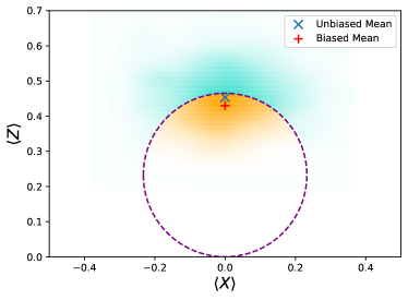
Figure 1: A geometric illustration of variance-bias tradeoff, displayed by the density of unbiased Pauli-$X$ and -$Z$ estimates averaged over $N_{s}=100$ samples each. For a biasing parameter of $\varepsilon=0.1$, the exterior of the dashed circle corresponds to the region where the biased estimate is closer to the true state than the unbiased one. The color of the density cloud thus represents the sign of the change in loss after biasing. Though the radius of the dashed circle is increasing with $\varepsilon$, it is compensated by the magnitude of the decrease in loss, so that biasing improves the estimate for $\varepsilon\leq\varepsilon_{\mathrm{min}}$. See details in Section C.1.

III Main Result

III.1 Biased shadow estimators

A channel $\widetilde{\mathcal{M}}$ that yields an unbiased estimator for the density matrix satisfies the condition $(\widetilde{\mathcal{M}}\circ\mathcal{M})[\rho]=\rho$ for all states $\rho$, and thus guarantees $\widetilde{\mathcal{M}}=\mathcal{M}^{-1}$ as

$$\mathds{E}_{\mathcal{U},\mathbf{b}}[\hat{\rho}]=(\widetilde{\mathcal{M}}\circ\mathcal{M})[\rho]\mathrm{.}$$ (2)

However, in the present work we focus on constructing a biased estimator which does not necessarily satisfy the above property but in return allows us to reduce the variance of the estimator.

To simplify our presentation, we illustrate our results on the simple uniform ensemble over $n$-qubit product Clifford rotations $\mathcal{U}=\mathcal{C}^{\times n}_{1}$. This is equivalent to uniformly sampling a local Pauli basis in which to measure each qubit and thus $\widetilde{\mathcal{M}}$ is a product channel and acts as

$$\hat{\rho}_{\ell} =\bigotimes_{j=1}^{n}\Big{[}3(U^{(j)}_{i})^{\dagger}|b^{(j)}\rangle\langle b^{(j)}|U^{(j)}_{i}-\openone\Big{]}$$ (3)

$$\equiv\bigotimes_{j=1}^{n}\widetilde{\mathcal{M}}_{\mathrm{local}}[(U^{(j)}_{i})^{\dagger}|b^{(j)}\rangle\langle b^{(j)}|U^{(j)}_{i}]\mathrm{.}$$ (4)

As the effect of $\mathcal{M}_{\mathrm{local}}$ is to contract the single-qubit Bloch sphere uniformly by a factor of 3, the inverse channel is given by dilating the Bloch sphere by the same factor. Our scheme biases this channel by effectively dilating the Bloch sphere by a smaller factor tuned via a bias parameter $\varepsilon$.

Statement 1 (biased shadow estimators).

Given a bias parameter $\varepsilon$ we modify the conventional shadow estimator in Eq. 2 and define the biased local estimator of Pauli shadows $\mathcal{M}^{(\varepsilon)}_{\mathrm{local}}$ as

$$\mathcal{M}^{(\varepsilon)}_{\mathrm{local}}(\rho)=3\sqrt{1-\varepsilon}\rho+\frac{1}{2}\left(1-3\sqrt{1-\varepsilon}\right)\mathds{1}\mathrm{.}$$ (5)

This channel dilates the Bloch sphere by a factor $3\sqrt{1-\varepsilon}$ and, indeed, for $\varepsilon=0$ we recover the unbiased channel of conventional classical shadows.

While the above channel does not converge to the true state in the infinite-sample limit for fixed (independent of $N_{s}$) $\varepsilon\neq 0$, it allows us to control shot noise (statistical uncertainty) in the finite-sample regime as the variance is decreased by $(1-\varepsilon)$. As we argue, by choosing the optimal $\varepsilon$ as a function of $N_{s}$, we obtain a consistent estimator, which converges to the unbiased estimate in the infinite-sample limit.

We now show that this trade-off is on average worthwhile through defining the expected loss as a measure of the average performance of the biased scheme as

$$\mathcal{L}_{\mathcal{U}}(\rho,\varepsilon)=\mathds{E}_{\mathcal{U},\mathbf{b}}\{\mathrm{tr}[(\rho-\hat{\rho})^{2}]\}.$$ (6)

In Fig. 1, we consider applying the Pauli shadows approach to estimating local properties of a quantum system and consider the reduced density matrix of a single-qubit. We fix a number of shots (samples) $N_{s}=100$, a biasing parameter of $\varepsilon=0.1$, and the true state $\rho$ on the $Z$-axis of the Bloch sphere. We calculate the change in loss for a set of averaged classical-shadow estimates of $\rho$ under biasing by $\varepsilon$. The exterior of the dashed circle corresponds to estimates where the corresponding biased estimator is actually more accurate in the particular finite-sample regime than the original, unbiased one. We now concretely state our analytical result that quantifies the expected loss for any particular local density matrix.

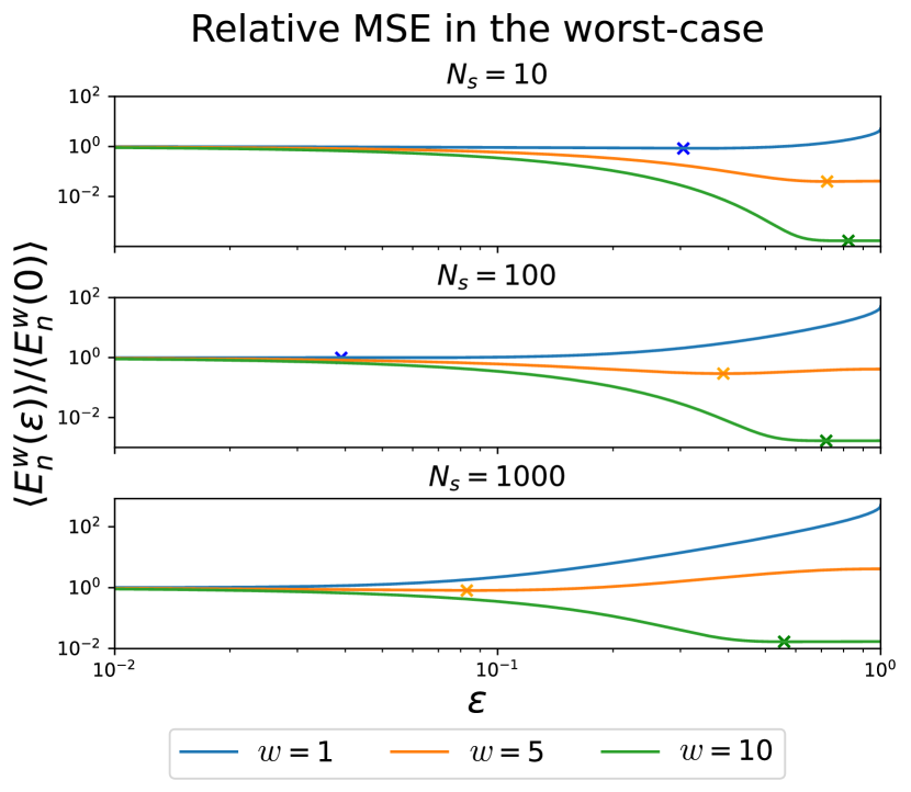
Figure 2: Mean squared error $\langle E_{n}^{\text{w}}(\varepsilon)\rangle$ of the biased scheme relative to the unbiased one when the aim is to estimate Pauli expected values $\mathrm{tr}(O\rho)$. Analytical expression plotted for the worst case scenario ($O$ commutes with $\rho$) for an increasing number of shots, weight of the Pauli string ($n=w$) and bias parameters $\varepsilon$. There is an optimal $\varepsilon$ (crosses at the minimum of the curves) for which the relative error is minimised. When $w=1$ and $N_{s}=1000$ the minimum is attained outside the plotted region.

Statement 2 (single-shot average-case loss).

For a single-qubit local density matrix $\rho=\tfrac{1}{2}[\mathds{1}+(\boldsymbol{r}\cdot\boldsymbol{\sigma})]$, where $\mathcal{U}$ forms a 2-design, the expected loss for a single sample is

$$\mathcal{L}_{\mathcal{U}}(\rho,\varepsilon)=\frac{1}{2}\left[\lVert\boldsymbol{r}\rVert^{2}+9(1-\varepsilon)\right]-\sqrt{1-\varepsilon}\lVert\boldsymbol{r}\rVert^{2}.$$ (7)

This is a quadratic expression in $\sqrt{1-\varepsilon}$ and thus attains a minimum value at $\sqrt{1-\varepsilon_{\mathrm{min}}}=\frac{1}{9}\lVert\boldsymbol{r}\rVert^{2}$ as

$$\mathcal{L}_{\mathcal{U}}(\rho,\varepsilon_{\mathrm{min}})=\frac{1}{18}\lVert\boldsymbol{r}\rVert^{2}\left(9-\lVert\boldsymbol{r}\rVert^{2}\right)$$ (8)

Thus, even if $\rho$ is pure ($\lVert\boldsymbol{r}\rVert=1$), it is worth introducing a strong bias for a single shot estimator as $\varepsilon_{\mathrm{min}}=\frac{80}{81}$ because it reduces the expected loss to $4/9$ from the expected loss $4$ of the unbiased scheme. However, in practice the qubit is usually part of an entangled (computational) state ($\lVert\boldsymbol{r}\rVert<1$) which guarantees even more significant gains. In the following sections we explain, however, that the gain is less pronounced as we increase the number of shots.

III.2 Analysing worst- and best-case gain

While in 2 we focused on the average performance of biased shadow tomography, we now analytically predict the performance in extremal scenarios. In particular, we consider the practically pivotal task of predicting expected values of local Pauli observables from the snapshots as $\mathrm{tr}(O\hat{\rho})$ and analyse the worst- and best-case scenarios. We note that we focus on the mean estimator, which is then of course the primary component of the median-of-means estimator [11].

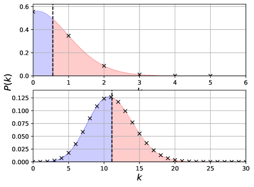
Figure 4: Binomial distribution for $p=1/9$, $N_{s}=5$ (top) and $N_{s}=100$ (bottom). For a small $N_{s}$, it is more likely to obtain an outcome larger than the mean (black dashed line) which leads to a high mean-squared error which can be reduced by biasing the estimator. When $N_{s}$ gets larger, biasing doesn’t improve our estimates as the distribution becomes symmetric around the mean.

As we will conclude below Eq. 12, our biased estimator yields the least gain in the worst-case scenario that the quantum state $\rho$ is the eigenstate of the Pauli observable via $\mathrm{tr}(O\rho)=+1$ (where $O$ is a Pauli string of weight $w$ up to $\pm$ sign). The reason why we still gain even in this worst-case scenario is the following: at each shot our estimator $\mathrm{tr}(O\hat{\rho})$ yields the outcome either $+1$ (when we measure in a compatible Pauli basis) or $0$ (when we measure in an incompatible basis). This indeed yields a binomial distribution $B(N_{s},p)$ with number of samples $N_{s}$ and probability of compatible measurements $p=3^{-w}$. As we illustrate in the Appendix (Fig. 4), the binomial distribution is not symmetric around the mean but has a tail, and the mean squared error on the right-hand side is higher than the mean squared error on the left-hand side – it is thus always worth biasing the estimator by effectively rescaling the estimate. However, as we increase $N_{s}$, the binomial distribution quickly tends to a symmetric normal distribution and thus rescaling will not yield an advantage.

In Appendix C we analytically derive the mean error $\langle E_{n}^{\text{w}}(\varepsilon)\rangle$ in the expected value measurement and plot these relative to the unbiased case in Fig. 2. Indeed, this confirms that (a) The biased scheme is always advantageous as there is always an optimal $\varepsilon$ (the minimum of the curves indicated using crosses) for which the relative mean error is smaller than $1$. (b) The advantage of the biased scheme grows exponentially as we increase the weight of the Pauli string simply because the contraction of the Bloch sphere is exponential via the factor $3^{w}$ for locality $w$ while the tail of the distribution of estimates (via the aforementioned binomial distribution) gets exponentially long, i.e., compare blue, orange and green lines. (c) The advantage of the biased scheme diminishes as we increase the numbers of shots.

In contrast, the best case scenario is attained when the quantum state is an eigenstate of an operator that anticommutes with the observable which gives us $\Tr(O\rho)=0$. It is then clear that biasing, which is equivalent to shrinking the expectation value is always advantageous as it forces the estimate to be closer to $0$. In Appendix C, we give an expression for the mean error $\langle E_{n}^{\text{b}}(\varepsilon)\rangle$ which we numerically compute and plot in Fig. 5 confirming that indeed increasing the bias parameter $\varepsilon$ monotonically decreases the expected error.

III.3 Relation to variances and quantum mechanical expected values

In the previous section we analysed the instances when the expected values attain the extremal values $\mathrm{tr}(O\rho)=\pm 1$ and $\mathrm{tr}(O\rho)=0$, and we now prove that indeed these are the worst- and best-case scenarios, respectively. For this reason we consider an arbitrary sample mean estimator $\overline{R}$ that one obtains from averaging over $N_{s}$ samples of a single-shot estimator $\hat{R}$, and compare $\overline{R}$ to the corresponding biased estimator $(1-\alpha)\overline{R}$ that one obtains through rescaling with the factor $(1-\alpha)$. In order to derive the optimal biasing point, i.e., the minimum of the curves in Fig. 2 (crosses), we first consider the Mean Squared Error (MSE) of the unbiased estimator $\overline{R}$ as ${\mathrm{MSE}[\overline{R}]}={\mathrm{Var}[\hat{R}]}/N_{s}$. We can define and calculate the Signal to Noise Ratio (SNR) of $\overline{R}$ as

$$\beta:=\frac{{\mathbb{E}[\overline{R}]}^{2}}{{\mathrm{MSE}[\overline{R}]}}=\frac{{\mathbb{E}[\hat{R}]}^{2}}{{\mathrm{Var}[\hat{R}]}/N_{s}}.$$ (9)

The MSE for the biased mean estimator $(1-\alpha)\overline{R}$ is then

$${\mathrm{MSE}[(1-\alpha)\overline{R}]}=\underbrace{\alpha^{2}{\mathbb{E}[\hat{R}]}^{2}}_{\text{bias}}+\underbrace{(1-\alpha)^{2}{\mathrm{Var}[\hat{R}]}/N_{s}}_{\text{variance}},$$ (10)

which is minimised at the optimal biasing point $\alpha^{*}~{}=~{}(1+\beta)^{-1}$ as we derive in Appendix D. Through Eq. 9, we find that the optimal bias parameter approaches $\alpha^{*}\rightarrow 0$ as we increase the number of samples $N_{s}\rightarrow\infty$. As such, our (optimally) biased estimator is actually a consistent estimator, i.e., it asymptotically approaches an unbiased estimator in the infinite-sample limit [18].

We can make the following statement at the optimal biasing point.

Statement 3 (biasing an estimator through rescaling).

The SNR of the optimally-biased estimator is $\beta_{\mathrm{biased}}=1+\beta$ which always guarantees an improved SNR over the unbiased estimator $\beta$. The relative SNR gain through biasing is given as

$$\frac{\beta_{\mathrm{biased}}}{\beta}=1+\beta^{-1}$$ (11)

As further shown in Appendix D, in the case of estimating Pauli expected values for Pauli shadows, the mean and variance of the single-shot estimator are given as ${\mathbb{E}[\hat{R}]}=\mathrm{tr}[O\rho]$ and ${\mathrm{Var}[\hat{R}]}=3^{w}-\mathrm{tr}[O\rho]^{2}$. Hence, the SNR of the unbiased estimator is given as $\beta=N_{s}[3^{w}\mathrm{tr}[O\rho]^{-2}-1]^{-1}$ and the factor of SNR gain by biasing is given by:

$$\frac{\beta_{\mathrm{biased}}}{\beta}=1+(3^{w}\mathrm{tr}[O\rho]^{-2}-1)/N_{s}$$ (12)

The maximal and minimal gains are then obtained at $\mathrm{tr}[O\rho]=0$ and $\mathrm{tr}[O\rho]=+1$ respectively, which proves our previous observations on worst- and best-case scenarios.

Let us note that, while the above SNR allows us to rigorously prove that biasing is in principle always advantageous, the mean-squared error analysed in the previous section remains the more practical measure and we will use it thereafter. It is also worth noting that Eq. 11 requires us to know the expectation value ${\mathbb{E}[\hat{R}]}$ exactly—which may not be possible in practice—in order to predict the optimal biasing point. Nevertheless, we demonstrate in the following section that biasing is still worthwhile even if we can only have approximate knowledge of the optimal bias.

IV Practical demonstration

We consider a potential practical application whereby one aims to obtain the ground-state energy of a Hamiltonian $\mathcal{H}$ composed of only low-weight (local) Pauli observables. In an experiment one first prepares the ground state and collects a set of Pauli shadows from which the ground-state energy can be predicted in post-processing. The significant advantage of classical shadows is that they allow us to estimate further Pauli strings beyond the Hamiltonian terms, without repeating the experiment.

For example, one can consider perturbative corrections to the Hamiltonian in the form of high-weight Pauli strings $P$ and predict the expected value of the sum $\mathcal{H}+P$, such as when computing a first-order correction to the energy in perturbation theory. However, the variance in our example is increased exponentially due to the high weight of $P$; this potentially renders a direct estimation impractical as the increased variance may bring the SNR down below $1$, as we detail in Appendix E. As we demonstrate, biasing then allows us to significantly improve upon this potentially low SNR.

As a concrete example we consider a spin-ring Hamiltonian as

$$\mathcal{H}=\sum_{k\in\text{ring}(N)}\omega_{k}Z_{k}+J\vec{\sigma}_{k}\cdot\vec{\sigma}_{k+1},$$ (13)

with coupling $J=0.3$, on-site interaction strengths uniformly randomly generated in the range $-1\leq\omega_{k}\leq 1$ and $\vec{\sigma}_{k}=(\sigma^{x}_{k},\sigma^{y}_{k},\sigma^{z}_{k})^{T}$ is a vector of single-qubit Pauli matrices. We prepare the ground state $\rho$ of a $12$-qubit Hamiltonian through a variational Hamiltonian ansatz of $l=5$ layers. We generate a collection of shadows $S(N_{s},\rho)$ with $N_{s}=10^{6}$ and estimate the expected value $\mathrm{tr}[(\mathcal{H}+P)\rho]$ with respect to corrections $P$ as $w=8$ Pauli observables.

In Fig. 3, we plot the mean-squared error obtained by averaging over $10^{5}$ repetitions and consider different $8$-local observables with and without biasing (blue). We consider two different biasing strategies. First, we analytically choose the optimal bias parameter $\alpha^{*}$ according to Eq. 11 (green) assuming direct access to the exact expected values (which one does not have access to in practice). Second, we use the experimentally estimated expected values to estimate the optimal biasing point in Eq. 11. While the latter deviates from the exact $\alpha^{*}$ due to shot noise, Fig. 3 (orange) clearly demonstrates that the MSE is still significantly reduced compared to the unbiased scheme. This confirms robustness against errors in our ability to determine the optimal bias parameter, i.e., the approach can demonstrably be used even when the optimal biasing point can only be estimated from the experimental data.

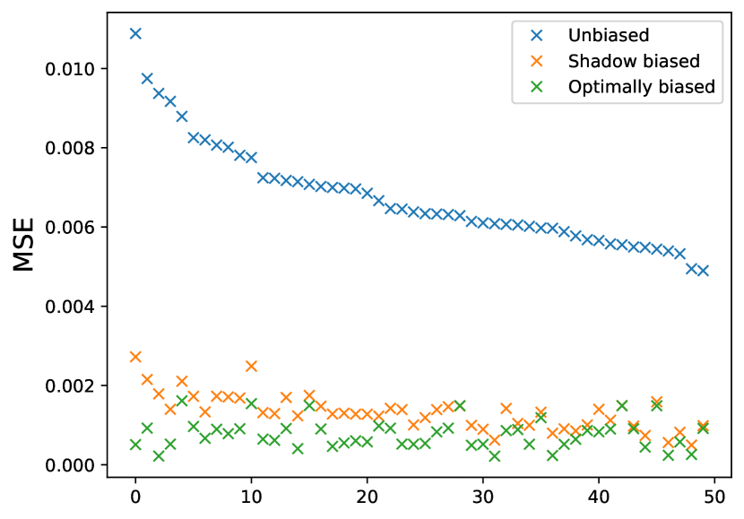
Figure 3: Illustration of the impact of different biasing strategies. In blue, we plot the MSE of fifty 8-local observables (whose SNR is smaller than $1$) sorted by how large the error is. While analytically choosing the optimal bias according to Eq. 11 drastically reduces the error (green), this assumes previous knowledge of the exact expectation values, which is not available in practice. Through estimating the optimal bias from experimental data (orange), one still obtains a significant error reduction.

V Discussion and Conclusion

In this work, we explore the tradeoff between intentionally introducing a bias into classical shadows estimators which in return allows us to reduce statistical uncertainties due to finite samples – ultimately enabling us to achieve the same precision but using fewer samples. The implementation of the approach is straightforward, and is performed completely in post-processing, as it is effectively just a rescaling of the conventional shadow estimator.

We obtain rigorous analytical guarantees that biasing is, in principle, always worthwhile given an optimal bias parameter is known: First, optimal biasing improves the relative loss of shadow tomography on average. Second, optimal biasing improves expected value measurements even in the worst-case scenario and may provide significant gains in other scenarios. Third, optimal biasing is guaranteed to increase the signal-to-noise of any statistical mean estimator. Although the optimal bias parameter is not known a priori, we demonstrate in a practically motivated numerical experiment that an approximation directly determined form experimental data is sufficient.

The gain using our biased estimator is more pronounced for a small number of samples or when Pauli strings of high weight are predicted. As such, our approach is thus particularly well suited for practical tasks where only a relatively low number of shots is available, e.g., estimating gradients [19, 20, 21, 22] or covariances [23] when training variational circuits or when estimating time-dependent properties [24]. Another particularly interesting application area is quantum error mitigation [25] whereby prior works aimed at recovering an unbiased estimator from noisy measurements. Combinations of QEM and classical shadows have similarly been considered [26, 27].

The insights and theoretical results provided in this work may prove invaluable in developing further, more advanced biased estimators. Given classical information from quantum systems can only be extracted through statistical estimators, this work is an important step in the crucial task of developing applications of quantum computers that have minimal sample requirements.

Appendix A Comparison to previous literature

The idea of introducing a bias in the context of classical shadows has been explored in several previous works, and here we compare our results to some notable examples.

In Ref. [32], the authors consider biasing the local measurement bases at the measurement stage of preparing classical shadows (i.e. choosing measurements from a biased distribution $\mathcal{U}$ over local basis rotations $U_{i}$). These authors then choose the biasing distribution to minimize the variance and report an unbiased estimator for the energy of a molecular Hamiltonian, expressed as a sum of Pauli strings. In Ref. [33], the authors introduce a biased estimator for the energy of a Pauli Hamiltonian by truncating the set of Pauli estimators included in the sum of the energy estimator. This bias is chosen based on the number of compatible measurement settings in a given measurement scheme, and is guaranteed to achieve the optimal tradeoff between the statistical error and the systematic error introduced by biasing. In both Refs. [32] and [33], the authors are considering estimating a single observable given by a sum of Pauli operators, as opposed to estimating multiple independent observables simultaneously.

In Ref. [34], the authors show that least-squares and regularized least-squares estimators can be viewed as instances of classical shadows that are generally biased. The authors note that an essential conceptual difference between the least-squares estimators and conventional classical shadows is that classical shadows make use of a hypothetical distribution from which unitary rotations are drawn. Our approach can be seen as incorporating this source of randomness together with bias.

Appendix B Average case loss

In this section, we show the following result for a single qubit

$$\mathds{E}_{\mathcal{U},\mathrm{b}}\{\mathrm{tr}[(\rho-\hat{\rho})^{2}]\}=\frac{1}{2}[\lVert\boldsymbol{r}\rVert^{2}+9(1-\varepsilon)]-\sqrt{1-\varepsilon}\lVert\boldsymbol{r}\rVert^{2}\mathrm{,}$$ (14)

where

$$\hat{\rho}=\mathcal{M}^{(\varepsilon)}\left[U\outerproduct{\mathrm{b}}{\mathrm{b}}U^{\dagger}\right]\mathrm{,}\mbox{\hskip 28.45274pt}\rho=\frac{1}{2}(I+\boldsymbol{r}\cdot\boldsymbol{\sigma})\mathrm{,}$$ (15)

and $\mathcal{U}$ is a Haar 2-design. We have

$$\mathds{E}_{\mathcal{U},\mathrm{b}}\{\mathrm{tr}[(\rho-\hat{\rho})^{2}]\} =\sum_{\mathrm{b}\in\mathds{Z}_{2}}\int_{\mathcal{U}}dU\ \bra{\mathrm{b}}U^{\dagger}\rho U\ket{\mathrm{b}}\mathrm{tr}\{[\rho-\mathcal{M}^{(\varepsilon)}(U\outerproduct{\mathrm{b}}{\mathrm{b}}U^{\dagger})]^{2}\}$$ (16)

Since $\mathcal{M}^{(\varepsilon)}$ only rescales the Bloch vector, the identity parts of $\rho$ and $\hat{\rho}$ cancel, and we have

$$\mathds{E}_{\mathcal{U},\mathrm{b}}\{\mathrm{tr}[(\rho-\hat{\rho})^{2}]\} =\frac{1}{4}\sum_{\mathrm{b}\in\mathds{Z}_{2}}\int_{\mathcal{U}}dU\ \bra{\mathrm{b}}U^{\dagger}\rho U\ket{\mathrm{b}}\mathrm{tr}\{[\left(\boldsymbol{r}\cdot\boldsymbol{\sigma}\right)-3(-1)^{\mathrm{b}}\sqrt{1-\varepsilon}\left(UZU^{\dagger}\right)]^{2}\}$$ (17)

$$\mathds{E}_{\mathcal{U},\mathrm{b}}\{\mathrm{tr}[(\rho-\hat{\rho})^{2}]\} =\frac{1}{4}\sum_{\mathrm{b}\in\mathds{Z}_{2}}\int_{\mathcal{U}}dU\ \bra{\mathrm{b}}U^{\dagger}\rho U\ket{\mathrm{b}}\mathrm{tr}\{[\lVert\boldsymbol{r}\rVert^{2}+9(1-\varepsilon)]I-6(-1)^{\mathrm{b}}\sqrt{1-\varepsilon}\left(UZU^{\dagger}\right)\left(\boldsymbol{r}\cdot\boldsymbol{\sigma}\right)\}$$ (18)

Inside of the trace, we have a term which is proportional to the identity, and a term which is proportional to the operator $(UZU^{\dagger})(\boldsymbol{r}\cdot\boldsymbol{\sigma})$. Calculating each one at a time, we have

$$(\mathrm{identity\ term}) =\frac{1}{4}\sum_{\mathrm{b}\in\mathds{Z}_{2}}\int_{\mathcal{U}}dU\ \bra{\mathrm{b}}U^{\dagger}\rho U\ket{\mathrm{b}}\mathrm{tr}\{[\lVert\boldsymbol{r}\rVert^{2}+9(1-\varepsilon)]I\}$$ (19)

$$=\frac{1}{2}[\lVert\boldsymbol{r}\rVert^{2}+9(1-\varepsilon)]$$ (20)

and

$$(\mathrm{non-identity\ term}) =-\frac{3}{2}\sqrt{1-\varepsilon}\sum_{\mathrm{b}\in\mathds{Z}_{2}}(-1)^{\mathrm{b}}\int_{\mathcal{U}}dU\ \bra{\mathrm{b}}U^{\dagger}\rho U\ket{\mathrm{b}}\mathrm{tr}\{\left(UZU^{\dagger}\right)\left(\boldsymbol{r}\cdot\boldsymbol{\sigma}\right)\}$$ (21)

$$=-\frac{3}{2}\sqrt{1-\varepsilon}\sum_{\mathrm{b}\in\mathds{Z}_{2}}(-1)^{\mathrm{b}}\mathrm{tr}\left\{\mathcal{E}^{(2)}\left(\outerproduct{\mathrm{b}}{\mathrm{b}}\otimes Z\right)\left[\rho\otimes\left(\boldsymbol{r}\cdot\boldsymbol{\sigma}\right)\right]\right\}$$ (22)

$$=-\frac{3}{2}\sqrt{1-\varepsilon}\mathrm{tr}\left\{\mathcal{E}^{(2)}\left(Z\otimes Z\right)\left[\rho\otimes\left(\boldsymbol{r}\cdot\boldsymbol{\sigma}\right)\right]\right\}$$ (23)

$$=-\frac{1}{2}\sqrt{1-\varepsilon}\mathrm{tr}\left\{\left(2S-I\right)\left[\rho\otimes\left(\boldsymbol{r}\cdot\boldsymbol{\sigma}\right)\right]\right\}$$ (24)

$$(\mathrm{non-identity\ term}) =-\sqrt{1-\varepsilon}\lVert\boldsymbol{r}\rVert^{2}$$ (25)

where $\mathcal{E}^{(2)}(A)=\int_{\mathcal{U}}dUU^{\otimes 2}A(U^{\otimes 2})^{\dagger}$, and $S$ is the 2-qubit SWAP operation. Therefore

$$\mathds{E}_{\mathcal{U},\mathrm{b}}\{\mathrm{tr}[(\rho-\hat{\rho})^{2}]\}=\frac{1}{2}[\lVert\boldsymbol{r}\rVert^{2}+9(1-\varepsilon)]-\sqrt{1-\varepsilon}\lVert\boldsymbol{r}\rVert^{2}$$ (26)

This is a quadratic expression in $\sqrt{1-\varepsilon}$, so it attains a minimum value at

$$\sqrt{1-\varepsilon_{\mathrm{min}}}=\frac{1}{9}\lVert\boldsymbol{r}\rVert^{2}\mbox{\hskip 14.22636pt}\mathrm{with}\mbox{\hskip 14.22636pt}\mathds{E}_{\mathcal{U},\mathrm{b}}\{\mathrm{tr}[(\rho-\widetilde{\rho})^{2}]\}|_{\varepsilon_{\mathrm{min}}}=\frac{1}{2}\lVert\boldsymbol{r}\rVert^{2}-\frac{1}{18}\lVert\boldsymbol{r}\rVert^{4}$$ (27)

Therefore, we can in-fact minimize the expected loss and decrease the classical-shadow sampling variance by introducing a biased inverse channel.

Appendix C Analysing worst and best-case scenarios

C.1 Single qubit error

Figure 1 depicts an approximate probability distribution of Bloch-vector estimates for a single qubit, each taken from the average of $N_{s}=100$ samples, again with unitaries drawn from $\mathcal{U}=\mathcal{C}_{1}$ and projected onto the $\left\langle X\right\rangle$, $\left\langle Z\right\rangle$ plane. Each of the estimates in this plot is unbiased, and we consider how biasing by $\varepsilon=0.1$ as described in the previous section would affect every estimate. The exterior of the dashed circle in the figure designates the region where the biased estimate has a lower expected loss to the true mean value than the unbiased one. At precisely zero bias, this curve would be a circle with the unbiased mean and the origin at opposite points of the circle on a diameter. As we increase $\varepsilon$, the radius of the circle increases such that the unbiased mean is moved into its interior (biasing the true mean value always results in higher loss), but the origin and the unbiased mean still lie on a diameter of the circle. When we include the $\left\langle Y\right\rangle$ value, this circle becomes a sphere of revolution about the common diameter defined by the origin and the unbiased mean.

We obtain an expected advantage from biasing our estimate when the increase in loss due to the estimates inside the dashed circle is outweighed by the decrease in loss due to the estimates outside. While increasing the bias decreases the probability mass outside of the circle, the probability mass that remains outside can enjoy a greater decrease in its loss. Intuitively, this is due to the geometry of the sphere and the fact that biasing pulls the estimates to the center. The region outside of the dashed circle includes a region where the error in all three Bloch vector components is decreased by biasing, whereas for every estimate inside the dashed circle, the error in at most one Bloch vector component is increased.

C.1.1 Worst case

The worst case scenario happens when the studied quantum state $\rho$ is an eigenstate of the Pauli observable of interest $O$. For ease of presentation, let us focus first on the single-qubit case. We generalise the following results to $n$-qubit states in the next subsection. Without loss of generality, let $\rho=\outerproduct{+}{+}$ and $O=X$ which thus satisfies $\mathrm{tr}(O\rho)=1$. For a given collection of shadows $S(\rho,N_{s})=\{\hat{\rho}_{1},\dots,\hat{\rho}_{N_{s}}\}$, our estimate for the expectation value is given by the mean of each snapshot’s expectation value,

$$\frac{1}{N_{s}}\sum_{i=1}^{N_{s}}\mathrm{tr}(X\hat{\rho}_{i}).$$ (28)

Each $\hat{\rho}_{i}$ has been obtained by measuring in a randomly chosen single-qubit Pauli basis, and as a result $\mathrm{tr}(X\hat{\rho}_{i})$ yields either $+1$ (when we measure in the Pauli $X$ basis) or $0$ (when we measure in the $Y$ or $Z$ bases). Here we aim to calculate the mean error made in computing the expectation value $\langle E_{1}^{\text{w}}(\varepsilon)\rangle$ when using a bias parameter $\varepsilon$. Suppose that $k$ snapshots resulted in the outcome $+1$ while $N_{s}-k$ resulted in the outcome $0$, we define the error in the mean value as,

$$E_{1}^{\text{w}}(\varepsilon) \coloneqq\left|\frac{1}{N_{s}}\sum_{i=1}^{N_{s}}\mathrm{tr}(X\hat{\rho}_{i})-1\right|^{2}=\left|\frac{3\sqrt{1-\varepsilon}}{N_{s}}k-1\right|^{2}.$$ (29)

The average error is then given by,

$$\langle E_{1}^{\text{w}}(\varepsilon)\rangle=\sum_{k=0}^{N_{s}}P\left(\sum_{i=1}^{N_{s}}\mathrm{tr}(X\hat{\rho}_{i})=k\right)\left|\frac{3\sqrt{1-\varepsilon}}{N_{s}}k-1\right|^{2},$$ (30)

where $\sum_{i=1}^{N_{s}}\mathrm{tr}(X\hat{\rho}_{i})$ is simply a random variable following a binomial distribution $B(N_{s},p)$ with $p=\tfrac{1}{3}$. We can then obtain an analytic expression for $P\left(\sum_{i=1}^{N_{s}}\mathrm{tr}(X\hat{\rho}_{i})=k\right)$ leading to,

$$\langle E_{1}^{\text{w}}(\varepsilon)\rangle=\sum_{k=0}^{N_{s}}{N_{s}\choose{k}}p^{k}(1-p)^{(N_{s}-k)}\left|\frac{3\sqrt{1-\varepsilon}}{N_{s}}k-1\right|^{2}.$$ (31)

C.1.2 Best case

The best case scenario is obtained when the state is an eigenstate of an operator that anticommutes with our observable, such as $\rho=\outerproduct{+}{+}$ and $O=Z$ which gives us $\mathrm{tr}(O\rho)=0$. For each sample our estimator yields either $+1$ or $-1$ with equal probability (compatible measurement in the Pauli $Z$ basis) or yields $0$ (incompatible measurement via Pauli $X$ and $Y$ bases). Again, we can compute the mean error over the distribution of $k$ as

$$\langle E_{1}^{\text{b}}(\varepsilon)\rangle=\sum_{k=-N_{s}}^{N_{s}}P\left(\sum_{i=1}^{N_{s}}\mathrm{tr}(Z\hat{\rho}_{i})=k\right)\left|\frac{3\sqrt{1-\varepsilon}}{N_{s}}k\right|^{2}.$$ (32)

With $P(\mathrm{tr}(Z\hat{\rho}_{i})=0)=\tfrac{2}{3}$ and $P(\mathrm{tr}(Z\hat{\rho}_{i})=1)=P(\mathrm{tr}(Z\hat{\rho}_{i})=-1)=\tfrac{1}{6}$. Finding an analytic formula for $P\left(\sum_{i=1}^{N_{s}}\mathrm{tr}(Z\hat{\rho}_{i})=k\right)$ is quite challenging, but one can easily compute it numerically. In Fig. 5, we compute the relative mean squared error between the biased and unbiased cases by sampling Eq. 32 $N_{reps}=10^{6}$ times for different values of $N_{s}$. The plot confirms our intuition that increasing the bias monotonically decreases the error.

Figure 5: Numerical evaluation of the mean squared error $\langle E_{1}^{\text{b}}(\varepsilon)\rangle$ of the biased scheme relative to the unbiased one when the aim is to estimate Pauli expected values $\mathrm{tr}(O\rho)$ in the best-case scenario for an increasing number of shots $N_{s}$ and bias parameters $\varepsilon$. As $\mathrm{tr}(O\rho)=0$ and biasing corresponds to shrinking the expectation value, we always reduce the relative error.

C.2 Multiqubit error

The generalisation to the multiqubit case is straightforward as both the initial state and observable can be written as tensor products. Let $\rho=\outerproduct{+}{+}^{\otimes n}$ and $O=X^{\otimes n}$, with $n$ the number of qubits. For a given collection of shadows $S(\rho,N_{s})=\{\hat{\rho}_{1},\dots,\hat{\rho}_{N_{s}}\}$ such that $\forall i,\hat{\rho}_{i}=\otimes_{j=1}^{n}\hat{\rho}_{i,j}$ the error in the worst-case now reads,

$$\langle E_{n}^{\text{w}}(\varepsilon)\rangle=\sum_{k=0}^{N_{s}}P\left(\sum_{i=1}^{N_{s}}\left(\prod_{j=1}^{n}\mathrm{tr}(X\hat{\rho}_{i,j})\right)=k\right)\left|\frac{3\sqrt{1-\varepsilon}}{N_{s}}k-1\right|^{2}.$$ (33)

Here $\sum_{i=1}^{N_{s}}\left(\prod_{j=1}^{n}\mathrm{tr}(X\hat{\rho}_{i,j})\right)\sim B(N_{s},p_{n})$ with $p_{n}=\tfrac{1}{3^{n}}$. Hence,

$$\langle E_{n}^{\text{w}}(\varepsilon)\rangle=\sum_{k=0}^{N_{s}}{N_{s}\choose{k}}p_{n}^{k}(1-p_{n})^{(N_{s}-k)}\left|\frac{3\sqrt{1-\varepsilon}}{N_{s}}k-1\right|^{2}.$$ (34)

Plotting $\langle E_{n}^{\text{w}}(\varepsilon)\rangle$ in Fig. 2 for different scenarios, we find that it is always worth biasing our estimator.

In the best case, with $\rho=\outerproduct{+}{+}^{\otimes n}$ and $O=Z^{\otimes n}$ we find,

$$\langle E_{n}^{\text{b}}(\varepsilon)\rangle=\sum_{k=-N_{s}}^{N_{s}}P\left(\sum_{i=1}^{N_{s}}\left(\prod_{j=1}^{n}\mathrm{tr}(Z\hat{\rho}_{i,j})\right)=k\right)\left|\frac{3\sqrt{1-\varepsilon}}{N_{s}}k\right|^{2},$$ (35)

Here again, one will need to numerically compute the error.

Appendix D Statistical Analysis for Biased Shadow

D.1 Biasing an estimator by rescaling

Suppose the target parameter that we want to estimate can be obtained using some unbiased estimator $\hat{R}$ with the corresponding sample mean estimator after $N_{s}$ shots denoted as $\overline{R}$. In this way, the mean square error (MSE) of the this unbiased estimator after $N_{s}$ shots is simply

$${\mathrm{MSE}[\overline{R}]}={\mathrm{Var}[\overline{R}]}={\mathrm{Var}[\hat{R}]}/N_{s}.$$ (36)

The error of the unbiased estimator is just the shot noise ${\mathrm{MSE}[\overline{R}]}={\mathrm{Var}[\hat{R}]}/N_{s}$, thus we can define the signal-to-noise ratio (SNR) of the unbiased shadow mean estimator as:

$$\beta=\frac{{\mathbb{E}[\overline{R}]}^{2}}{{\mathrm{MSE}[\overline{R}]}}=\frac{{\mathbb{E}[\hat{R}]}^{2}}{{\mathrm{Var}[\hat{R}]}/N_{s}}.$$ (37)

Note that $\beta^{-\frac{1}{2}}$ is the fractional error of the unbiased shadow estimator.

We want to see if we can reduce this MSE by simply rescaling $\hat{R}$, which gives rise to the biased estimator $(1-\alpha)\hat{R}$. The MSE of this biased estimator after $N_{s}$ shots is:

$$\quad{\mathrm{MSE}[(1-\alpha)\overline{R}]}$$

$$=\underbrace{\left({\mathbb{E}[(1-\alpha)\hat{R}]}-{\mathbb{E}[\hat{R}]}\right)^{2}}_{\text{bias}}+\underbrace{{\mathrm{Var}[(1-\alpha)\hat{R}]}/N_{s}}_{\text{variance}}$$

$$=\alpha^{2}{\mathbb{E}[\hat{R}]}^{2}+(1-\alpha)^{2}{\mathrm{Var}[\hat{R}]}/N_{s}.$$ (38)

To obtain the minimum MSE, we can take the derivative with respect to $\alpha$ and setting it to zero:

$$2\alpha^{*}{\mathbb{E}[\hat{R}]}^{2}-2(1-\alpha^{*}){\mathrm{Var}[\hat{R}]}/N_{s}=0$$

$$\alpha^{*}=\frac{{\mathrm{Var}[\hat{R}]}/N_{s}}{{\mathbb{E}[\hat{R}]}^{2}+{\mathrm{Var}[\hat{R}]}/N_{s}}=\frac{1}{1+\beta}.$$ (39)

The MSE at this optimal point can be obtained by substituting the expression of $\alpha^{*}$ back into the MSE expression, which gives

$${\mathrm{MSE}[(1-\alpha^{*})\overline{R}]} =\frac{{\mathbb{E}[\hat{R}]}^{2}{\mathrm{Var}[\hat{R}]}/N_{s}}{{\mathbb{E}[\hat{R}]}^{2}+{\mathrm{Var}[\hat{R}]}/N_{s}}=\alpha^{*}{\mathbb{E}[\hat{R}]}^{2}.$$ (40)

Using this, we can obtain the SNR of the optimal biased shadow mean estimator:

$$\beta_{\mathrm{biased}}=\frac{{\mathbb{E}[\hat{R}]}^{2}}{{\mathrm{MSE}[(1-\alpha^{*})\overline{R}]}}=\alpha^{*-1}=1+\beta.$$ (41)

This is always larger than $1$ regardless of how small the unbiased SNR $\beta$ is, i.e. using the optimal bias scheme, we can always obtain an SNR larger than $1$ for all estimators! This is definitely not true for the unbiased estimator, e.g. in the case of local Clifford shadows that we will see later, the unbiased SNR $\beta$ decays exponentially with the weight of the observable.

For estimators that have large unbiased SNR $\beta\gg 1$, the improvement of the SNR from $\beta$ to $1+\beta$ by biasing is marginal. While for unbiased estimators that contain mostly noise $\beta\ll 1$, optimal biasing can always extract useful signal by increasing the SNR to above $1$.

D.2 Local Clifford Shadow

In the context of shadow estimation, we are predicting the expected value of a weight-$w$ observable $O$ from shadows as the mean of the random variable

$$\hat{R}=\mathrm{tr}[O\hat{\rho}].$$ (42)

Here $\hat{\rho}$ is a snapshot of the shadow protocol.

More exactly, in the post-processing step, we prepare some stabiliser state based on the shadow and then measure the Pauli observable $O$ to obtain some random variable $\hat{Q}$, then we rescale the result by a factor of $3^{w}$ to obtain the biased-free shadow estimator $\hat{R}=3^{w}\hat{Q}$. In local Clifford shadow procedure, the probability that $O$ coincides with one of the stabilisers modulo phase (the measurement basis of the shadow) is $3^{-w}$. In this case, the output from measuring $O$ on the stabiliser state is simply a Pauli random variable $\hat{O}$ with outcomes $\pm 1$, which means that $\hat{O}^{2}=1$. For the rest of the time, $O$ is not in the stabilisers modulo phase, and the output from measuring $O$ on the stabiliser state is simply $0$. Hence, we have

$${\mathbb{E}[\hat{Q}]} =3^{-w}{\mathbb{E}[\hat{O}]}+(1-3^{-w})0=3^{-w}{\mathbb{E}[\hat{O}]},$$

$${\mathbb{E}[\hat{Q}^{2}]} =3^{-w}{\mathbb{E}[\hat{O}^{2}]}+(1-3^{-w})0^{2}=3^{-w},$$

$${\mathrm{Var}[\hat{Q}]} ={\mathbb{E}[\hat{Q}^{2}]}-{\mathbb{E}[\hat{Q}]}^{2}=3^{-w}-3^{-2w}{\mathbb{E}[\hat{O}]}^{2}.$$

Using $\hat{R}=3^{w}\hat{Q}$, we have

$${\mathbb{E}[\hat{R}]} =3^{w}{\mathbb{E}[\hat{Q}]}={\mathbb{E}[\hat{O}]},$$ (43)

$${\mathrm{Var}[\hat{R}]} =3^{2w}{\mathrm{Var}[\hat{Q}]}=3^{w}-{\mathbb{E}[\hat{R}]}^{2},$$ (44)

Eq. 43 should not come as a surprise because both $\hat{R}$ and $\hat{O}$ are unbiased estimators of our target expectation value, it is just that $\hat{R}$ is obtained from the shadow procedure while $\hat{O}$ is obtain from direct measurement on the state.

In this way, we can simplify the unbiased shadow SNR in Eq. 37 to:

$$\beta =\frac{{\mathbb{E}[\hat{R}]}^{2}}{{\mathrm{MSE}[\overline{R}]}}=\frac{N_{s}{\mathbb{E}[\hat{R}]}^{2}}{3^{w}-{\mathbb{E}[\hat{R}]}^{2}}=N_{s}\left(\frac{3^{w}}{{\mathbb{E}[\hat{R}]}^{2}}-1\right)^{-1},$$ (45)

which fits our intuition that the SNR will increase as we increase the number of shots $N_{s}$, decrease the observable weight $w$ and/or have large expectation value ${\mathbb{E}[\hat{R}]}$.

D.3 Critical Biasing

For the biased shadow estimator to outperform the unbiased one, we have:

$${\mathrm{MSE}[(1-\alpha)\hat{R}]} \leq{\mathrm{MSE}[\hat{R}]}$$

$$\alpha^{2}{\mathbb{E}[\hat{R}]}^{2}+(1-\alpha)^{2}{\mathrm{Var}[\hat{R}]}/N_{s} \leq{\mathrm{Var}[\hat{R}]}/N_{s}$$

$$\alpha^{2}{\mathbb{E}[\hat{R}]}^{2} \leq\alpha(2-\alpha){\mathrm{Var}[\hat{R}]}/N_{s}.$$

One trivial solution here is $\alpha=0$. If we focus on the $\alpha>0$ case, we then have:

$$\alpha{\mathbb{E}[\hat{R}]}^{2} \leq(2-\alpha){\mathrm{Var}[\hat{R}]}/N_{s}$$

$$\alpha \leq\frac{2{\mathrm{Var}[\hat{R}]}/N_{s}}{{\mathbb{E}[\hat{R}]}^{2}+{\mathrm{Var}[\hat{R}]}/N_{s}}=\alpha_{c}.$$

We note that $\alpha_{c}=2\alpha^{*}$. All the simplified expression of $\alpha^{*}$ using $\hat{R}=3^{w}\hat{Q}$ will also apply to $\alpha_{c}$.

Appendix E Possible application scenarios for biased shadow

Here let us outline a situation where biasing might help. Suppose we try to estimate the energy $E$ of a quantum state by measuring some low-weight observable $A$ on the shadow of the state. The expectation value of $A$ can be estimated using the shadows from the estimator $\overline{A}$, and we have measure enough shadow shots such that ${\mathrm{Var}[\overline{A}]}$ is small. At a later stage, we suddenly realise that there should be a higher-order correction in the form of high-weight observable $R$ with the corresponding estimator from our existing shadow denoted as $\overline{R}$. i.e. we have

$$E={\mathbb{E}[\overline{A}]}+{\mathbb{E}[\overline{R}]}.$$

However, due to the high weight of the high-order correction, its variance (noise) exceed the amount of signal the it contains, i.e. its SNR is smaller than $1$:

$${\mathbb{E}[\overline{R}]}^{2}/{\mathrm{Var}[\overline{R}]}=\beta\leq 1.$$

This implies that without biasing, including this higher order correction $\overline{R}$ will include more noise than signal. Hence, we are better off simply using $\overline{A}$ as our estimator for $E$ without including $\overline{R}$. The corresponding MSE of using $\overline{A}$ to estimate $E$ is

$${\mathrm{MSE}[\overline{A}]}_{E}={\mathrm{Var}[\overline{A}]}+\underbrace{{\mathbb{E}[\overline{R}]}^{2}}_{\text{bias}}.$$

As mentioned, we can increase the SNR for any estimator to above $1$ by biasing it. If we use the optimal biasing scheme for the estimation of ${\mathbb{E}[\overline{R}]}$, this will in turn give us the following estimator for $E$:

$$\overline{H}=\overline{A}+(1-\alpha^{*})\overline{R}.$$

Using Eq. 40, we have

$${\mathrm{MSE}[\overline{H}]}_{E} ={\mathrm{Var}[\overline{A}]}+{\mathrm{MSE}[(1-\alpha^{*})\overline{R}]}$$

$$={\mathrm{Var}[\overline{A}]}+\alpha^{*}{\mathbb{E}[\overline{R}]}^{2}.$$

As mentioned before, for the original estimator $\overline{A}$ we usually have enough shots such that ${\mathrm{Var}[\overline{A}]}$ is very small, thus it is likely to be the case that the higher-order correction is the error bottleneck. In this case, we can simplify the MSE of the two estimators of $E$ to

$${\mathrm{MSE}[\overline{A}]}_{E} ={\mathbb{E}[\overline{R}]}^{2}$$

$${\mathrm{MSE}[\overline{H}]}_{E} =\alpha^{*}{\mathbb{E}[\overline{R}]}^{2}.$$

i.e. through biasing the higher-order correction, we can include it and reduce the MSE by a factor of $\alpha^{*-1}=1+\beta$. As mentioned, the SNR of the higher-order correction was $\beta\leq 1$. Hence, we can achieve up to $2$ times reduction in the MSE in this case.

References

- Arute et al. [2019] F. Arute, K. Arya, R. Babbush, D. Bacon, J. C. Bardin, R. Barends, R. Biswas, S. Boixo, F. G. S. L. Brandao, D. A. Buell, B. Burkett, Y. Chen, Z. Chen, B. Chiaro, R. Collins, W. Courtney, A. Dunsworth, E. Farhi, B. Foxen, A. Fowler, C. Gidney, M. Giustina, R. Graff, K. Guerin, S. Habegger, M. P. Harrigan, M. J. Hartmann, A. Ho, M. Hoffmann, T. Huang, T. S. Humble, S. V. Isakov, E. Jeffrey, Z. Jiang, D. Kafri, K. Kechedzhi, J. Kelly, P. V. Klimov, S. Knysh, A. Korotkov, F. Kostritsa, D. Landhuis, M. Lindmark, E. Lucero, D. Lyakh, S. Mandrà, J. R. McClean, M. McEwen, A. Megrant, X. Mi, K. Michielsen, M. Mohseni, J. Mutus, O. Naaman, M. Neeley, C. Neill, M. Y. Niu, E. Ostby, A. Petukhov, J. C. Platt, C. Quintana, E. G. Rieffel, P. Roushan, N. C. Rubin, D. Sank, K. J. Satzinger, V. Smelyanskiy, K. J. Sung, M. D. Trevithick, A. Vainsencher, B. Villalonga, T. White, Z. J. Yao, P. Yeh, A. Zalcman, H. Neven, and J. M. Martinis, Quantum supremacy using a programmable superconducting processor, Nature 574, 505 (2019).
- Wu et al. [2021] Y. Wu, W.-S. Bao, S. Cao, F. Chen, M.-C. Chen, X. Chen, T.-H. Chung, H. Deng, Y. Du, D. Fan, M. Gong, C. Guo, C. Guo, S. Guo, L. Han, L. Hong, H.-L. Huang, Y.-H. Huo, L. Li, N. Li, S. Li, Y. Li, F. Liang, C. Lin, J. Lin, H. Qian, D. Qiao, H. Rong, H. Su, L. Sun, L. Wang, S. Wang, D. Wu, Y. Xu, K. Yan, W. Yang, Y. Yang, Y. Ye, J. Yin, C. Ying, J. Yu, C. Zha, C. Zhang, H. Zhang, K. Zhang, Y. Zhang, H. Zhao, Y. Zhao, L. Zhou, Q. Zhu, C.-Y. Lu, C.-Z. Peng, X. Zhu, and J.-W. Pan, Strong Quantum Computational Advantage Using a Superconducting Quantum Processor, Physical Review Letters 127, 180501 (2021).
- Zhong et al. [2021] H.-S. Zhong, Y.-H. Deng, J. Qin, H. Wang, M.-C. Chen, L.-C. Peng, Y.-H. Luo, D. Wu, S.-Q. Gong, H. Su, Y. Hu, P. Hu, X.-Y. Yang, W.-J. Zhang, H. Li, Y. Li, X. Jiang, L. Gan, G. Yang, L. You, Z. Wang, L. Li, N.-L. Liu, J. J. Renema, C.-Y. Lu, and J.-W. Pan, Phase-Programmable Gaussian Boson Sampling Using Stimulated Squeezed Light, Physical Review Letters 127, 180502 (2021).
- Bluvstein et al. [2023] D. Bluvstein, S. J. Evered, A. A. Geim, S. H. Li, H. Zhou, T. Manovitz, S. Ebadi, M. Cain, M. Kalinowski, D. Hangleiter, J. P. B. Ataides, N. Maskara, I. Cong, X. Gao, P. S. Rodriguez, T. Karolyshyn, G. Semeghini, M. J. Gullans, M. Greiner, V. Vuletić, and M. D. Lukin, Logical quantum processor based on reconfigurable atom arrays, Nature , 1 (2023).
- Kim et al. [2023] Y. Kim, A. Eddins, S. Anand, K. X. Wei, E. van den Berg, S. Rosenblatt, H. Nayfeh, Y. Wu, M. Zaletel, K. Temme, and A. Kandala, Evidence for the utility of quantum computing before fault tolerance, Nature 618, 500 (2023).
- ach [2023] Suppressing quantum errors by scaling a surface code logical qubit, Nature 614, 676 (2023).
- Sugiyama et al. [2013] T. Sugiyama, P. S. Turner, and M. Murao, Precision-guaranteed quantum tomography, Phys. Rev. Lett. 111, 160406 (2013).
- Guţă et al. [2020] M. Guţă, J. Kahn, R. Kueng, and J. A. Tropp, Fast state tomography with optimal error bounds, Journal of Physics A: Mathematical and Theoretical 53, 204001 (2020).
- Meyer et al. [2023] J. J. Meyer, S. Khatri, D. Stilck França, J. Eisert, and P. Faist, Quantum metrology in the finite-sample regime, arXiv e-prints , arXiv:2307.06370 (2023), arXiv:2307.06370 [quant-ph] .
- Elben et al. [2023] A. Elben, S. T. Flammia, H.-Y. Huang, R. Kueng, J. Preskill, B. Vermersch, and P. Zoller, The randomized measurement toolbox, Nature Reviews Physics 5, 9 (2023).
- Huang et al. [2020] H.-Y. Huang, R. Kueng, and J. Preskill, Predicting many properties of a quantum system from very few measurements, Nature Physics 16, 1050 (2020).
- Huang et al. [2021] H.-Y. Huang, R. Kueng, and J. Preskill, Efficient Estimation of Pauli Observables by Derandomization, Phys. Rev. Lett. 127, 030503 (2021), arXiv:2103.07510 [quant-ph] .
- Zhao et al. [2021] A. Zhao, N. C. Rubin, and A. Miyake, Fermionic partial tomography via classical shadows, Phys. Rev. Lett. 127, 110504 (2021).
- Wan et al. [2022] K. Wan, W. J. Huggins, J. Lee, and R. Babbush, Matchgate Shadows for Fermionic Quantum Simulation, arXiv e-prints , arXiv:2207.13723 (2022), arXiv:2207.13723 [quant-ph] .
- Chen et al. [2021] S. Chen, W. Yu, P. Zeng, and S. T. Flammia, Robust shadow estimation, PRX Quantum 2, 030348 (2021).
- Nguyen et al. [2022] H. C. Nguyen, J. L. Bönsel, J. Steinberg, and O. Gühne, Optimizing shadow tomography with generalized measurements, Phys. Rev. Lett. 129, 220502 (2022).
- Ferrie and Blume-Kohout [2018] C. Ferrie and R. Blume-Kohout, Maximum likelihood quantum state tomography is inadmissible, arXiv e-prints , arXiv:1808.01072 (2018), arXiv:1808.01072 [quant-ph] .
- Scott and Wu [1981] A. Scott and C.-F. Wu, On the asymptotic distribution of ratio and regression estimators, Journal of the American Statistical Association 76, 98 (1981).
- Schuld et al. [2019] M. Schuld, V. Bergholm, C. Gogolin, J. Izaac, and N. Killoran, Evaluating analytic gradients on quantum hardware, Physical Review A 99, 032331 (2019).
- Koczor and Benjamin [2022a] B. Koczor and S. C. Benjamin, Quantum analytic descent, Physical Review Research 4, 023017 (2022a).
- Wierichs et al. [2022] D. Wierichs, J. Izaac, C. Wang, and C. Y.-Y. Lin, General parameter-shift rules for quantum gradients, Quantum 6, 677 (2022).
- Koczor and Benjamin [2022b] B. Koczor and S. C. Benjamin, Quantum natural gradient generalized to noisy and nonunitary circuits, Physical Review A 106, 062416 (2022b).
- Boyd and Koczor [2022] G. Boyd and B. Koczor, Training variational quantum circuits with covar: Covariance root finding with classical shadows, Phys. Rev. X 12, 041022 (2022).
- Chan et al. [2022] H. H. S. Chan, R. Meister, M. L. Goh, and B. Koczor, Algorithmic shadow spectroscopy, arXiv preprint arXiv:2212.11036 (2022).
- Cai et al. [2023] Z. Cai, R. Babbush, S. C. Benjamin, S. Endo, W. J. Huggins, Y. Li, J. R. McClean, and T. E. O’Brien, Quantum error mitigation, Reviews of Modern Physics 95, 045005 (2023).
- Jnane et al. [2024] H. Jnane, J. Steinberg, Z. Cai, H. C. Nguyen, and B. Koczor, Quantum error mitigated classical shadows, PRX Quantum 5, 010324 (2024).
- Zhao and Miyake [2023] A. Zhao and A. Miyake, Group-theoretic error mitigation enabled by classical shadows and symmetries, arXiv preprint arXiv:2310.03071 (2023).
- Jones et al. [2019] T. Jones, A. Brown, I. Bush, and S. C. Benjamin, QuEST and High Performance Simulation of Quantum Computers, Scientific Reports 9, 10736 (2019).
- Jones and Benjamin [2020] T. Jones and S. Benjamin, Questlink—mathematica embiggened by a hardware-optimised quantum emulator*, Quantum Science and Technology 5, 034012 (2020).
- Meister [2022] R. Meister, pyQuEST - A Python interface for the Quantum Exact Simulation Toolkit (2022).
- Richards [2015] A. Richards, University of Oxford Advanced Research Computing (2015).
- Hadfield et al. [2022] C. Hadfield, S. Bravyi, R. Raymond, and A. Mezzacapo, Measurements of quantum hamiltonians with locally-biased classical shadows, Communications in Mathematical Physics 391, 951 (2022).
- Gresch and Kliesch [2023] A. Gresch and M. Kliesch, Guaranteed efficient energy estimation of quantum many-body Hamiltonians using ShadowGrouping, arXiv e-prints , arXiv:2301.03385 (2023), arXiv:2301.03385 [quant-ph] .
- Zhu et al. [2023] Z. Zhu, J. M. Lukens, and B. T. Kirby, On the connection between least squares, regularization, and classical shadows, arXiv e-prints (2023), arXiv:2310.16921 [quant-ph] .