Dynamic modeling and predictive control
of a microfluidic system

Abstract

Microfluidics, the study of fluids in microscopic channels, has led to important advances in fields as diverse as microelectronics, biotechnology and chemistry. Microfluidic research is primarily based on the use of microfluidic chips, low-cost devices that can be used to perform laboratory experiments using small amounts of fluid. These systems, however, require advanced control mechanisms in order to accurately achieve the flow rates and pressures required in the experiments. In this paper, we present the design of a model predictive controller intended to regulate the fluid flows in one of these systems. The results obtained, both through simulations and real experiments performed on the device, show that predictive control is an ideal technique to control these systems, especially taking into account all the existing constraints.

I Introduction

The study of fluids under conditions where they flow through a network of micrometer-sized channels is known as microfluidics. Microfluidic systems are primarily based on the use of small chips, known as labs-on-a-chip, in which a variety of physical, chemical, or biological processes can be replicated. These systems have been applied in numerous fields such as chemistry, biotechnology, or medical research (Ohno et al., 2008; Gómez et al., 2016; Méndez Pérez et al., 2011). Microfluidics has made it possible, for example, to make advances in disease diagnosis or the simulation of organ behavior in small devices (Wang et al., 2021; Li et al., 2022). It also makes it possible to more realistically recreate the environment of certain microorganisms, allowing the study of more complex cultures. Another application where these devices stand out is in three-dimensional cell culture, where physiological conditions can be more reliably replicated (Duinen et al., 2015). Ultimately, this technology enables tests that provide more accurate results and reduce the need for animal experimentation. In addition, the use of these devices lowers the cost of carrying out certain experiments because the amount of chemicals required is very small, which also reduces the amount of waste generated.

The dynamics of microfluidic systems typically depend on several variables. Therefore, to fully exploit their potential, it is essential to develop and implement advanced control methods. Specifically, model predictive control (MPC) is a potential control strategy for these devices, as it allows the control of systems with multiple inputs and multiple outputs. Its main advantage is that it allows predicting the evolution of the process in the future, taking into account all the physical constraints of the process in the calculation of the control action, whether they are in the input, state, output, or all of them simultaneously. However, the use of this type of control involves a more complex development and implementation than classical controllers, as it is essential to perform tasks such as building a model or defining the cost function to minimize. In the literature, very diverse applications of this type of control can be found, from its use in resonant power converters (Lucia et al., 2021), to the cement industry (Clarke, 1988), improving the energy efficiency of air conditioning systems (Marchante et al., 2021), controlling solar plants (Gallego Len et al., 2022), or clinical anesthesia applications (Gómez et al., 2016; Méndez Pérez et al., 2011), just to name a few examples. Additionally, more innovative developments are also underway, such as the combination of predictive control with neural networks for nonlinear systems (Calle Chojeda et al., 2022). All these references show that model predictive control is increasingly being used in numerous scientific and industrial fields.

Returning to the specific field of microfluidics, various works related to the development of controllers for these systems can be found in the literature. For example, in Kim et al. (2013), a control system for a mechanical component of a microfluidic device is proposed, and in Kuczenski et al. (2007), a procedure is described to control the interface between two fluids in a microscopic channel. However, most of these systems rely on the use of PID controllers, whose limitations in managing constraints are widely known. For example, Heo et al. (2016), presents the design of a flow control algorithm and its comparison with a conventional PID controller, and Miller et al. (2010) describes a PID controller for a microfluidic droplet generation device. The alternative proposed by some authors is in fact the development of model predictive control systems. Examples can be found in droplet-based microfluidic systems (Maddala and Rengaswamy, 2013) or electroporation systems (Ghadami et al., 2013), although none of these proposals specifically apply MPC techniques for flow control. Special mention should also be made of certain works, such as that of García-Camprubí et al. (2020), focused specifically on the design of estimation algorithms intended for use in MPC controllers.

In this paper, we present the design of a model predictive controller for a microfluidic system. The objective is to control independently the flows circulating through three microscopic channels in a microfluidic chip, which meet at the same point to form a common outflow. This particular configuration is used in techniques such as Flow Focusing, which consists in the generation of droplets and is used in fields such as drug encapsulation or particle design (Martín-Banderas et al., 2005; Gañán Calvo, 1998). The system is subject to numerous constraints, both on flow rates and applied pressures. Additionally, the coupling between different variables and the complexity of the system itself make it difficult to control using classical techniques, which justifies the need for MPC control. Since only partial measurements are available, the controller relies on a state observer whose design is also presented in the paper. The results obtained, both through simulation and on the real system, demonstrate the benefits of the proposed control system.

The structure of the article is summarized as follows. Following this introductory section, Section II describes the microfluidic system under study. Subsequently, in Section III, we present the dynamic model of the complete system, as well as a simplified version used by the estimation and control algorithms. Sections IV and V describe, respectively, the state observer and the MPC controller designed. The results obtained with the complete implementation, first in simulation and then on the real system, are included in Section VI. Finally, Section VII presents the main conclusions of the work.

II System description

The microfluidic system used (see Fig. 1) consists of three pressure regulators (A), three compressed air lines (B), three liquid reservoirs (C), three fluid lines with their respective flow meters (D), the microfluidic chip (E), an outlet line (F), and a final liquid reservoir (G). Fig. 2 shows a real image of the chip used.

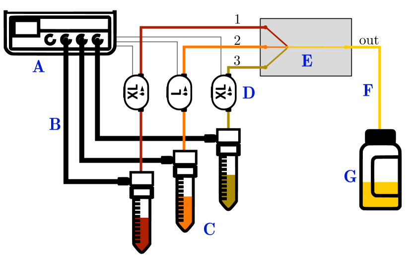
Figure 1: Schematic diagram of the microfluidic system used.

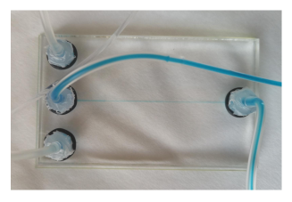
Figure 2: Photograph of the microfluidic chip.

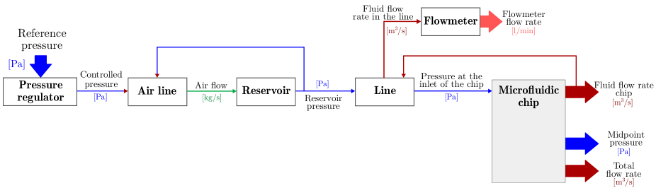
Figure 3: Conceptual block diagram for one of the lines.

Fig. 3 shows a conceptual block diagram for one of the lines, which is analogous to the three existing in the system. The system operation is as follows. The inputs are pressure references introduced to the regulators. These regulators act on the system to achieve, after a certain transient time, the requested pressures at the beginning of the compressed air lines. This pressure is transmitted to the reservoirs, which contain a fluid consisting of a mixture of water (74% by volume) and glycerin (26%), identical for all three lines. As a result of the pressure applied, the liquid contained in the reservoirs begins to flow through the fluid lines towards the chip. Next, the liquid enters the chip, where the three channels converge at a common point. Finally, all the fluid exits through the chip’s outlet channel to a line that connects it to a reservoir at atmospheric pressure. It is important to note that, in each of the three fluid lines between the reservoirs and the chip, the flow meters provide real-time measurements of the liquid flow rate. These measurements are the only ones used to close the control loop.

III System modeling

In this section, the equations of the dynamic model of the complete system presented in the previous section are presented. This model consists of the union of different submodels described in the following sections, each associated to a specific part of the system. It should be noted that a simplified version of this model is used for programming both the observer and the controller. The simplified model is described at the end of the section.

III-A Theoretical preliminaries

The most relevant parameters in a microfluidic line are its hydraulic resistance, $\mathcal{R}$, and inertia, $I$. The following expression can be used to calculate the inertia of a specific line,

$$I=\frac{\rho\;l}{A}\;,$$ (1)

where $l$ and $A$ are, respectively, the length and cross-sectional area of the line, and $\rho$ is the fluid density. The hydraulic resistance of rectangular channels can be calculated using the following expression (Rapp, 2017),

$$\mathcal{R}=\frac{12\,\mu\,l}{h^{3}\,w}\cdot\frac{1}{\left(1-\frac{192\,h}{\pi^{5}\,w}\right)\,\sum_{j=0}^{\infty}\left(\frac{1}{(2j+1)^{5}}\tanh\left(\frac{(2j+1)\,\pi\,w}{2\,h}\right)\right)},$$ (2)

where $\mu$ is the dynamic viscosity of the fluid, $h$ is the height of the channel’s cross-section, and $w$ is its width. On the other hand, for circular cross-section lines, the following expression is used (Rapp, 2017),

$$\mathcal{R}=\mu\cdot\frac{8\,l}{\pi\,r^{4}},$$ (3)

where $r$ is the radius of the cross-sectional area of the line.

Using Poiseuille’s law and the hydraulic-electrical analogy, the flow variation in the channels can be formulated as a function of the pressure difference between two points in the channel, $\Delta P$, the hydraulic resistance, $\mathcal{R}$, the flow rate through the channel, $Q$, and the fluid inertia in the channel, $I$. The hydraulic-electrical analogy allows some equations related to fluids to be reformulated by analogy with electrical equations. In this regard, an equivalence can be established between hydraulic resistance, $\mathcal{R}$, and electrical resistance, $R_{e}$; between flow rate, $Q$, and electrical current, $I_{e}$; between the pressure difference between two points, $\Delta P$, and voltage drop, $V_{e}$; and between the fluid inertia in the channel, $I$, and the inductance, $L$, of an electrical circuit.

$$\Delta P=\mathcal{R}\,Q+I\,\dot{Q}\qquad\longleftrightarrow\qquad V_{e}=R_{e}\,I_{e}+L\,\dot{I}_{e}\;$$ (4)

Another relevant equation in these systems is the one describing the dynamics of pressures. The variation of pressure in a volume is expressed as the flow balance in that volume divided by the compressibility (Bruus, 2007),

$$\dot{P}=\frac{\Delta Q}{C},$$ (5)

where $\Delta Q$ is the difference between the flow entering and leaving this volume, and $C$ is the compressibility of the fluid in the chamber under study, given by

$$C=\frac{V_{{tot}}}{E},$$ (6)

where $V_{{tot}}$ is the total volume of the chamber containing the fluid and $E$ is the bulk modulus of the fluid.

III-B Modeling of the microfluidic chip

The chip (see Fig. 4) consists of three rectangular cross-sectional input channels with their respective flow rates, $Q_{1}^{\,{chip}}$, $Q_{2}^{\,{chip}}$, and $Q_{3}^{\,{chip}}$, and one output channel with flow rate $Q_{{out}}$. The flow rates of the input lines are controlled by acting on the input pressures to the chip, $P_{1}^{\,{chip}}$, $P_{2}^{\,{chip}}$, and $P_{3}^{\,{chip}}$. A variable $P_{M}$ is defined for the pressure at the midpoint where the three input channels merge. It should be noted that this variable cannot be measured directly. The output of the chip is at atmospheric pressure, $P_{{atm}}$.

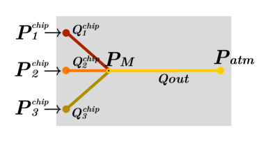
Figure 4: Chip diagram

Applying (4) to each of the three input channels of the chip, the expressions of the derivatives of the flow rates can be obtained,

$$\dot{Q}_{i}^{\,{chip}}=\frac{P_{i}^{\,{chip}}-P_{M}-\mathcal{R}_{i}^{\,{chip}}\,Q_{i}^{\,{chip}}}{I_{i}^{\,{chip}}},\hskip 14.22636pti\in\{1,2,3\}$$ (7)

where ${I_{i}^{\,{chip}}}$ and ${\mathcal{R}_{i}^{\,{chip}}}$ are the inertia and hydraulic resistance of the $i$-th channel of the chip, calculated respectively using (1) and (2). The dynamic equation for the output channel can be obtained similarly, in this case with atmospheric pressure at the outlet,

$$\dot{Q}_{{out}}=\frac{P_{M}-P_{{atm}}-\mathcal{R}_{{out}}\;Q_{{out}}}{I_{{out}}},$$ (8)

where $I_{{out}}$ and $\mathcal{R}_{{out}}$ are respectively the inertia and hydraulic resistance of the output channel.

The compressibility of the fluid in the chip, $C^{\,{chip}}$, can be obtained using (6). In this case, the total volume is the sum of the volumes of each of the input channels, $V_{i}^{{\,{chip}}}$, $i\in{1,2,3}$, and the output channel, $V_{{out}}$.

$$C^{\,{chip}}=\frac{V_{1}^{\,{chip}}+V_{2}^{\,{chip}}+V_{3}^{\,{chip}}+V_{{out}}}{E}$$ (9)

Besides, the pressure variation at the junction point of the lines can be obtained by applying (5) to the chip.

$$\dot{P}_{M}=\frac{Q_{1}^{\,{chip}}+Q_{2}^{\,{chip}}+Q_{3}^{\,{chip}}-Q_{{out}}}{C^{\,{chip}}}$$ (10)

III-C Modeling of the fluid lines and flow meters

For the lines connecting the reservoirs to the chip, the flow meter is considered to be part of the line. This implies that, for each line, the inertia, volume, and resistance are the sum of those corresponding to the line and the flow meter.

The flow through the line depends on the pressure difference between the two ends of the line. From (4), we obtain the following expressions for each of the three lines,

$$\dot{Q}_{i}^{{\,{line}}}=\frac{P_{i}^{\,{\,{res}}}-P_{i}^{\,{chip}}-\mathcal{R}_{i}^{{\,{line}}}\,Q_{i}^{{\,{line}}}}{I_{i}^{{\,{line}}}},\ i\in\{1,2,3\},$$ (11)

where $Q_{i}^{{\,{line}}}$ is the flow rate of the $i$-th fluid line, ${I_{i}^{\,{line}}}$ and ${\mathcal{R}_{i}^{\,{line}}}$ are the inertia and hydraulic resistance of said line, calculated in this case using (1) and (3) for having a circular section, and $P_{i}^{\,{\,{res}}}$ denotes the pressure of the $i$-th reservoir. The pressure variation at the end of each line can be obtained as a function of the flow rates by applying (5) to this case,

$$\dot{P}_{i}^{\,{chip}}=\frac{Q_{i}^{{\,{line}}}-Q_{i}^{\,{chip}}}{C_{i}^{{\,{line}}}},\hskip 14.22636pti\in\{1,2,3\},$$ (12)

where $C_{i}^{{\,{line}}}$ is the compressibility of the fluid in the $i$-th line, obtained from (6) as

$$C_{i}^{{\,{line}}}=\frac{V_{i}^{{\,{line}}}+V_{i}^{{\,{fm}}}+V_{i}^{{\,{chip}}}}{E}\approx\frac{V_{i}^{{\,{line}}}+V_{i}^{{\,{fm}}}}{E}.$$ (13)

In the previous expression, $V_{i}^{{\,{line}}}$ and $V_{i}^{{\,{fm}}}$ are, respectively, the volumes of the $i$-th line and its corresponding flow meter. To calculate the fluid compressibility $C_{i}^{{\,{line}}}$, the influence of the volume of each of the chip channels, $V_{i}^{{\,{chip}}}$, can be neglected as these are much smaller than those of the fluid lines and flow meters.

III-D Modeling of the reservoirs and air lines

The three reservoirs containing the liquid are supplied with pressurized air through a series of tubes. This air causes the liquid to exit through the previously described lines. The ideal gas law is used to model the dynamics of this part,

$$\dot{P}_{i}^{\,{\,{res}}}\,V_{i}^{\,{\,{res}}}=\dot{m}_{i}\,R\,T,\vspace{3mm}$$ (14)

where $\dot{m}_{i}$ is the mass flow rate of gas flowing through the $i$-th air duct and reaching each of the reservoirs, and $V_{i}^{\,{\,{res}}}$ is the volume of the corresponding reservoir. Both the volume occupied by the air in each reservoir, $V_{i}^{\,{\,{res}}}$, and the temperature, $T$, are assumed to be constant. For air, $R=287.14$ J/(kg·K) is assumed.

The mass flow rate of air through the tube is calculated using the isentropic flow model with adiabatic index $\gamma=1.4$ (Çengel et al., 2018; White, 2008),

$$\dot{m}_{i}=\frac{A^{{\,{duct}}}\,P_{i}^{\,{reg}}}{\sqrt{R\,T}}\;\sqrt{7\left(\frac{P_{i}^{\,{\,{res}}}}{P_{i}^{\,{reg}}}\right)^{{10}/{7}}\left[1-\left(\frac{P_{i}^{\,{\,{res}}}}{P_{i}^{\,{reg}}}\right)^{{2}/{7}}\right]},$$ (15)

where $A^{{\,{duct}}}$ is the cross-sectional area of the duct, $P_{i}^{\,{reg}}$ is the pressure at the beginning of the $i$-th air line (regulated by the corresponding pressure controller), and $P_{i}^{\,{\,{res}}}$ is the pressure at the end of the line (pressure in the $i$-th reservoir).

III-E Modeling of the pressure regulators

In the system used, there are three pressure regulators whose internal dynamics are a priori unknown. These regulators do not immediately provide the required pressure, but have their own dynamics that need to be modeled. In this case, we propose to use linear dynamic black-box models where the input is a pressure reference, ${u}_{i}$, and the output is the controlled pressure, $P_{i}^{\,{reg}}$.

In order to identify these systems, the Matlab System Identification Toolbox has been used to obtain a transfer function for each type of regulator by analyzing different sets of experimental data. The tests have been based on requesting different setpoints in the range of 0 to 150 000 Pa and recording the step response of the regulators. By observing the system output, it was determined that the most appropriate model for the regulator of line 2 is a second-order linear model. For the other two lines, a different behavior was observed, which fits better with a third-order dynamics. That is, their dynamics are given by

$${u}_{1} ={P}_{1}^{\,{reg}}+a_{1}\dot{P}_{1}^{\,{reg}}+a_{2}\ddot{P}_{1}^{\,{reg}}+a_{3}\dddot{P}_{1}^{\,{reg}},$$ (16)

$${u}_{2} ={P}_{2}^{\,{reg}}+b_{1}\dot{P}_{2}^{\,{reg}}+b_{2}\ddot{P}_{2}^{\,{reg}},$$ (17)

$${u}_{3} ={P}_{3}^{\,{reg}}+c_{1}\dot{P}_{3}^{\,{reg}}+c_{2}\ddot{P}_{3}^{\,{reg}}+c_{3}\dddot{P}_{3}^{\,{reg}},$$ (18)

where the coefficients $a_{1}$, $a_{2}$, $a_{3}$, $b_{1}$, $b_{2}$, $c_{1}$, $c_{2}$, and $c_{3}$ have also been estimated using the mentioned tool.

III-F Complete system model for simulation

From all the previous equations, it is possible to build a dynamic model of the whole system with the 22 state variables listed in Table I. This model, whose dynamics is nonlinear due to the use of equation (15), has as inputs the three pressure references provided to the pressure regulators, and as outputs, the three flow readings from the three flow meters installed in the lines.

In order to perform realistic simulations, this model was implemented in Matlab-Simulink, taking into account certain effects such as possible noise in the measurements or the internal dynamics of the flow meters. This implementation has been used to validate through simulation both the observer and the predictive controller proposed in this work.

TABLE I: State variables of the complete system.

Name	Description
$Q_{1}^{\,{chip}}$, $Q_{2}^{\,{chip}}$, $Q_{3}^{\,{chip}}$	Flow rates at the chip inlet
$Q_{{out}}$	Flow rate at the chip outlet
$P_{M}$	Pressure at the midpoint
$Q_{1}^{{\,{line}}}$, $Q_{2}^{{\,{line}}}$, $Q_{3}^{{\,{line}}}$	Flow rates in the lines
$P_{1}^{\,{chip}}$, $P_{2}^{\,{chip}}$, $P_{3}^{\,{chip}}$	Pressures at the chip inlet
${P}_{1}^{\,{\,{res}}}$, ${P}_{2}^{\,{\,{res}}}$, ${P}_{3}^{\,{\,{res}}}$	Pressures in the reservoirs
${P}_{1}^{\,{reg}},\dot{P}_{1}^{\,{reg}},\ddot{P}_{1}^{\,{reg}}$	Controlled pressure 1 and its derivatives
${P}_{2}^{\,{reg}},\dot{P}_{2}^{\,{reg}}$	Controlled pressure 2 and its derivative
${P}_{3}^{\,{reg}},\dot{P}_{3}^{\,{reg}},\ddot{P}_{3}^{\,{reg}}$	Controlled pressure 3 and its derivatives

III-G Simplification for observation and control

Based on the complete model, a simplification has been performed by grouping the whole system into a lower-order state-space model with linear dynamics. In this regard, it has been verified by simulation that neglecting the effect of the air reservoir and possible losses in it has minimal influence. Specifically, for a set point of 10 000 Pa applied equally to all three lines, the difference between the steady-state flow rates is less than $0.5\%$, calculated as the difference between the flow rate of the two models with respect to the flow rate of the complete system. This allows to reduce the complexity of the model used in the design of the observer and the controller by simplifying the nonlinear part, while leaving the rest with linear dynamics. Thus, the pressures ${P}_{i}^{\,{reg}}$ and ${P}_{i}^{\,{\,{res}}}$ are assumed to be equal for each of the three lines. It is also assumed that the flow rate through each line is equal to the flow rate through the corresponding channel inside the chip, i.e., $Q_{i}^{{\,{line}}}=Q_{i}^{\,{chip}}$. Since the flow meter is considered to be part of the line (see section III-C), the flow rate measured by it will directly correspond to the flow through the corresponding line and inside the chip.

Considering the above, the lines linking the reservoirs and the chip and the chip channels themselves are considered in the simplified model as a set, thus simplifying the pressures at the chip inlet, $P_{i}^{\,{chip}}$. That is, the simplified model assumes that the pressure at the inlet of the system composed of one of the lines and the corresponding internal channel of the chip is the controlled pressure ${P}_{i}^{\,{reg}}$. In making this union, the resistance and inertia properties of the assembly are given by

$$\left\{\begin{array}[]{r@{}l}\mathcal{R}_{i}&=(\mathcal{R}_{i}^{\,{chip}}+\mathcal{R}_{i}^{{\,{line}}})\\ I_{i}&=(I_{i}^{\,{chip}}+I_{i}^{{\,{line}}})\end{array}\right.\;\;\;\;\;\;i\in\{1,2,3\}.$$ (19)

With the simplification, the variables for intermediate pressures and flow rates in the lines are no longer used, reducing the number of state variables from 22 to 13 (see Table II). Furthermore, in subsequent analyses, to simplify the operations, all pressures are considered relative to atmospheric pressure, so $P_{{atm}}=0$ Pa is assumed in the model. The resulting model can be represented compactly as

$$\mathbf{\dot{x}_{m}}(t) =\mathbf{A_{m}}\,\mathbf{x_{m}}(t)+\mathbf{B_{m}}\,\mathbf{u}(t),$$ (20)

$$\mathbf{y}(t) =\mathbf{H_{m}}\,\mathbf{x_{m}}(t),$$ (21)

where $\mathbf{x_{m}}\in\mathbb{R}^{n}$, with $n=13$, is the state vector, formed by the state variables from Table II (in that order), and $\mathbf{u}\in\mathbb{R}^{m}$, with $m=3$, and $\mathbf{y}\in\mathbb{R}^{p}$, with $p=3$, are, respectively, the input and output vectors of the system, defined as:

$$\mathbf{u}=\left[u_{1}\;\ u_{2}\;\ u_{3}\right]^{T},\hskip 10.00002pt\mathbf{y}=\left[y_{1}\;\ y_{2}\;\ y_{3}\right]^{T}=\left[Q_{1}\;\ Q_{2}\;\ Q_{3}\right]^{T}.$$

The state ($\mathbf{A_{m}}$), input ($\mathbf{B_{m}}$), and output ($\mathbf{H_{m}}$) matrices of the model are not explicitly shown in this article due to space limitations. However, they can be directly obtained from the equations (7)–(19).

Regarding the accuracy of the simplification made, it has been verified by simulation that, given a constant set point of 150 000 Pa (the maximum supported by the system), the maximum difference in steady state between the flow rates of the complete and simplified models is less than 6.5% with respect to the system without simplification. During the transient response, there are slightly larger differences, but we have considered that the behavior is acceptable enough to use the simplified model.

This simplified model is used in the design of the controller and observer. Specifically, the implementation uses the discrete-time version of the model,

$$\mathbf{x_{m}}(k+1) =\mathbf{F_{m}}\,\mathbf{x_{m}}(k)+\mathbf{G_{m}}\,\mathbf{u}(k),$$ (22)

$$\mathbf{y}(k) =\mathbf{H_{m}}\,\mathbf{x_{m}}(k),$$ (23)

where $\mathbf{F_{m}}$ and $\mathbf{G_{m}}$ are, respectively, the state transition matrix and the input matrix in discrete time.

TABLE II: State variables of the simplified system.

Name	Description
$Q_{1}$, $Q_{2}$, $Q_{3}$	Flow rates in the line + channel assembly
$Q_{{out}}$	Flow rate at the chip outlet
$P_{M}$	Pressure at the midpoint
${P}_{1}^{\,{reg}},\dot{P}_{1}^{\,{reg}},\ddot{P}_{1}^{\,{reg}}$	Controlled pressure 1 and its derivatives
${P}_{2}^{\,{reg}},\dot{P}_{2}^{\,{reg}}$	Controlled pressure 2 and its derivatives
${P}_{3}^{\,{reg}},\dot{P}_{3}^{\,{reg}},\ddot{P}_{3}^{\,{reg}}$	Controlled pressure 3 and its derivatives

IV State observer

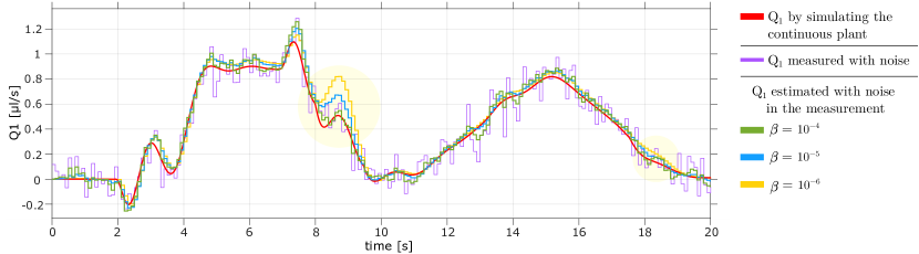
Figure 5: Simulation results of the Kalman filter performance in the presence of noise.

IV-A Observer design

The simplified model described previously has thirteen state variables, whose values need to be known in real time in order to control the system. In practice, however, it is not possible to measure all of them since the three available flow meters only allow for the measurement of three of these state variables. It is thus necessary to design and implement an observer that estimates the unmeasured variables in order to reconstruct the full state at each instant. In this work, the state observation is carried out using a Kalman filter. The filter is based on the classical formulation in Kalman (1960) and Welch and Bishop (2006), and it is described by the following equations:

$${\mathbf{x}^{\prime}_{\mathbf{m}}}(k) =\mathbf{F_{m}}\,\hat{\mathbf{x}}_{\mathbf{m}}(k-1)+\mathbf{G_{m}}\,\mathbf{u}(k-1),$$ (24)

$${\mathbf{P}^{\prime}}(k) =\mathbf{F_{m}}\,\hat{\mathbf{P}}(k-1)\,\mathbf{F_{m}}^{T}+\mathbf{Q_{\scriptscriptstyle KF}},$$ (25)

$${\mathbf{K}}(k) =\mathbf{P^{\prime}}(k)\,\mathbf{H_{m}}^{T}\left[\mathbf{H_{m}}\,\mathbf{P^{\prime}}(k)\,\mathbf{H_{m}}^{T}+\mathbf{R_{\scriptscriptstyle KF}}\right]^{-1},$$ (26)

$${\hat{\mathbf{x}}}_{\mathbf{m}}(k) =\mathbf{x}^{\prime}_{\mathbf{m}}(k)+\mathbf{K}(k)\left[\mathbf{y}(k)-\mathbf{H_{m}}\,\mathbf{x}^{\prime}_{\mathbf{m}}(k)\right],$$ (27)

$${\hat{\mathbf{P}}}(k) =\mathbf{P^{\prime}}(k)-\mathbf{K}(k)\,\mathbf{H_{m}}\,\mathbf{P^{\prime}}(k),$$ (28)

where ${\mathbf{x}^{\prime}_{\mathbf{m}}}$ and $\hat{\mathbf{x}}_{\mathbf{m}}$ are the a priori and a posteriori estimates of the state ${\mathbf{x}_{\mathbf{m}}}$, ${\mathbf{P}^{\prime}}$ and $\hat{\mathbf{P}}$ are the corresponding covariance matrices of these estimates, and $\mathbf{K}$ is the Kalman gain. Additionally, there are parameters that are crucial for the filter’s performance: the covariance matrices of the measurement noise, denoted as $\mathbf{R_{\scriptscriptstyle KF}}\in\mathbb{R}^{p\times p}$, and the process noise, denoted as $\mathbf{Q_{\scriptscriptstyle KF}}\in\mathbb{R}^{n\times n}$.

IV-B Simulation and tuning of the observer

In order to verify the correct design of the filter, several simulations have been carried out in the software Matlab-Simulink, with the complete model playing the role of the real system, modeled as previously indicated. However, the observer is based on the simplified model. Thus, in the simulation, the model of the system available to the observer is not exactly the same as that of the plant.

Based on preliminary tests on the system, it was determined that the measurement noise of the flow meters is in the range of $\pm\;0.3$ $\mu$l/s. Assuming Gaussianity and that this value corresponds to three standard deviations, it was concluded that the variance of the measurement noise should be about $10^{-20}$ (m³/s)². Consequently, considering that the three sensors are independent and thus the measurements must be uncorrelated, we decided to set $\mathbf{R_{\scriptscriptstyle KF}}=\mathbf{I}_{p}\cdot 10^{-20}$, where $\mathbf{I}_{p}$ is the identity matrix of size $p=3$.

For the definition of the matrix $\mathbf{Q_{\scriptscriptstyle KF}}$ it is assumed that the noise affecting each state variable in (22) is independent of the others. In other words, $\mathbf{Q_{\scriptscriptstyle KF}}$ is set to be diagonal. Furthermore, to determine its value, it has been assumed that such noise signals are Gaussian with zero mean and standard deviation proportional to a characteristic value of the corresponding variable. Therefore, the covariance of the process noise has the form

$$\mathbf{Q_{\scriptscriptstyle KF}} =\begin{bmatrix}\mathbf{Q_{\scriptscriptstyle KF}}_{Q}&\mathbf{0}_{4\times 9}\\ \mathbf{0}_{9\times 4}&\mathbf{Q_{\scriptscriptstyle KF}}_{P}\end{bmatrix},$$ (29)

where

$$\mathbf{Q_{\scriptscriptstyle KF}}_{Q}=\beta\cdot\begin{bmatrix}1&0&0&0\\ 0&1&0&0\\ 0&0&1&0\\ 0&0&0&9\end{bmatrix}\cdot 10^{-18}$$

is the submatrix of $\mathbf{Q_{\scriptscriptstyle KF}}$ associated with the flow rate variables, $\mathbf{Q_{\scriptscriptstyle KF}}_{P}=\beta\cdot\mathbf{I}_{9}\cdot 10^{8}$ is the submatrix corresponding to the pressures and their derivatives, $\beta$ is a dimensionless factor that allows adjusting the filter’s behavior, and $\mathbf{0}_{p\times n}$ is a matrix of zeros with $p$ rows and $n$ columns. Note that the different orders of magnitude arise from working with different magnitudes (pressures and flow rates) in very different numerical ranges.

When setting the value of $\beta$, a decision must be made whether to minimize the effect of noise, relying solely on the model of the plant available to the filter and sacrificing some measurement information, or to allow a minimal level of noise effect and improve the response to discrepancies in the plant. Fig. 5 shows the evolution of the flow rate $Q_{1}$ for different values of $\beta$. In all these simulations, measurement noise with the mentioned variance, i.e., $10^{-20}$ (m³/s)², has been artificially introduced. Successive simulations have allowed us to determine that the value of $\beta=$ $10^{-4}$ preserves the real behavior with a reduced noise effect. For higher values, too much confidence is placed in the simplified model, leading to errors (areas highlighted in yellow in the figure), while for lower values, too much noise is observed.

The simulations performed lead to the conclusion that the designed observer is valid for observing the system state variables even with some measurement noise. Based on the results, it is determined that in order to obtain the best performance, it would be advisable to adjust the matrices during the system calibration to best match the specific operating conditions. In cases where the system undergoes significant changes during operation, it would be appropriate to use an adaptive algorithm that modifies the model matrices according to the observations.

V MPC controller

V-A Controller design

The following is a description of the model predictive controller (MPC) design used for this system. One of the main strengths of this type of control is that the formulation allows for controlling multi-input, multi-output systems, including constraints on the input, state, or output in the formulation. Additionally, MPC allows for real-time optimization, explicitly using a plant model to predict the process evolution in future time steps by minimizing an objective function.

The formulation used in the implementation of the MPC controller in this system is based on that described in Wang (2009) and Camacho and Bordons (2010). This formulation utilizes the following extended model of the system,

$$\mathbf{x}(k+1) =\mathbf{F}\,\mathbf{x}(k)+\mathbf{G}\,\Delta\mathbf{u}(k),$$ (30)

$$\mathbf{y}(k) =\mathbf{H}\,\mathbf{x}(k),$$ (31)

where $\mathbf{x}$ is the extended state, defined as

$$\mathbf{x}(k)=\begin{bmatrix}\Delta\mathbf{x}_{\mathrm{m}}(k)\\ \mathbf{y}(k)\end{bmatrix}=\begin{bmatrix}\mathbf{x}_{\mathrm{m}}(k)-\mathbf{x}_{\mathrm{m}}(k-1)\\ \mathbf{y}(k)\end{bmatrix}.$$ (32)

It is important to note that the input to this model consists of control action increments, that is, $\Delta\mathbf{u}(k)=\mathbf{u}(k)-\mathbf{u}(k-1)$, rather than the control actions themselves. This implies that the MPC formulation implicitly includes an integrator for each output, allowing the desired setpoint to be reached in steady-state even in the presence of disturbances or modeling errors. The matrices $\mathbf{F}$, $\mathbf{G}$, and $\mathbf{H}$, which can be obtained by operating on (22)–(23), have the following form:

$$\mathbf{F}=\begin{bmatrix}\mathbf{F}_{\mathrm{m}}&\mathbf{0}^{T}_{p\times n}\\ \mathbf{H}_{\mathrm{m}}\mathbf{F}_{\mathrm{m}}&\mathbf{I}_{p}\end{bmatrix},\hskip 3.00003pt\mathbf{G}=\begin{bmatrix}\mathbf{G}_{\mathrm{m}}\\ \mathbf{H}_{\mathrm{m}}\mathbf{G}_{\mathrm{m}}\end{bmatrix},\hskip 3.00003pt\mathbf{H}=\begin{bmatrix}\mathbf{0}_{p\times n}&\mathbf{I}_{p}\end{bmatrix}.$$

In this work, we consider the control horizon and the prediction horizon to be equal, which we will simply refer to as the horizon and denote as $N$. Based on this horizon, it is possible to define the following vectors:

$$\Delta\mathbf{U}(k)=\begin{bmatrix}\Delta\mathbf{u}(k)\\[-3.0pt] \vdots\\ \Delta\mathbf{u}(k+N-1)\end{bmatrix}$$ (33)

$$\mathbf{Y}(k)=\begin{bmatrix}\mathbf{y}(k+1\,|\,k)\\[-3.0pt] \vdots\\ \mathbf{y}(k+N\,|\,k)\end{bmatrix}\quad\mathbf{Y_{d}}(k)=\begin{bmatrix}\mathbf{y_{d}}(k+1)\\[-3.0pt] \vdots\\ \mathbf{y_{d}}(k+N)\end{bmatrix},$$ (34)

where $\mathbf{y}(j\,|\,k)\in\mathbb{R}^{p}$ is the prediction of the system output at the $j$-th instant based on the information available at the $k$-th instant, and $\mathbf{y_{d}}(j)\in\mathbb{R}^{p}$ is the desired value for that output at that instant. In other words, the vectors $\Delta\mathbf{U}\in\mathbb{R}^{Nm}$, $\mathbf{Y}\in\mathbb{R}^{Np}$ and $\mathbf{Y_{d}}\in\mathbb{R}^{Np}$ contain, respectively, the control action increments, the predicted outputs, and the desired values for the whole horizon. Operating with these vectors and the model (30)–(31), it is possible to express the vector $\mathbf{Y}(k)$ as

$$\mathbf{Y}(k)=\mathbf{\Psi}\,\mathbf{x}(k)+\mathbf{\Phi}\,\Delta\mathbf{U}(k),$$ (35)

where $\mathbf{\Psi}$ and $\mathbf{\Phi}$ are constant matrices defined as

$$\mathbf{\Psi}\!=\!\!\begin{bmatrix}\mathbf{H}\mathbf{F}\\ \mathbf{H}\mathbf{F}^{2}\\[-3.0pt] \vdots\\[2.0pt] \mathbf{H}\mathbf{F}^{N}\end{bmatrix}\!,\,\mathbf{\Phi}\!=\!\!\begin{bmatrix}\mathbf{H}\mathbf{G}&\mathbf{0}_{p\times m}&\cdots&\mathbf{0}_{p\times m}\\ \mathbf{H}\mathbf{A}\mathbf{G}&\mathbf{H}\mathbf{G}&\cdots&\mathbf{0}_{p\times m}\\[-3.0pt] \vdots&\ddots&\ddots&\\[2.0pt] \mathbf{H}\mathbf{F}^{N-1}\mathbf{G}&\mathbf{H}\mathbf{F}^{N-2}\mathbf{G}&\cdots&\mathbf{H}\mathbf{G}\end{bmatrix}\!.$$

Based on the above definitions, the cost function to be minimized, $J$, is formulated as the sum of a tracking error term, which takes into account how far the flow rates are from the desired values, and another term associated with the increase in the control variable,

$$J(k)=\tilde{\mathbf{Y}}(k)^{T}\cdot\mathbf{W_{y}}\cdot\tilde{\mathbf{Y}}(k)+\Delta\mathbf{U}(k)^{T}\cdot\mathbf{W_{u}}\cdot\Delta\mathbf{U}(k),$$ (36)

where $\tilde{\mathbf{Y}}=\mathbf{Y}-\mathbf{Y_{d}}$ is the vector with the tracking errors. The diagonal matrix $\mathbf{W_{y}}\in\mathbb{R}^{Np\,\times\,Np}$ determines the importance of the error $\tilde{\mathbf{Y}}$ in $J$. Additionally, it also establishes the relative weights between the errors of the three outputs. In this case, the three outputs are flow rates that are within the same value ranges. Since the importance of the error is the same for all three, we decided to set all these values to unity. That is, $\mathbf{W_{y}}=\mathbf{I}_{Np}$. On the other hand, the diagonal matrix $\mathbf{W_{u}}\in\mathbb{R}^{Nm\,\times\,Nm}$ allows to define the relative weights of the control actions, both among themselves and with respect to the term associated with the error $\tilde{\mathbf{Y}}$. Since in the system under studye the three actions are pressures within the same value ranges, and the relative importance is the same for all three, we decided that all the elements of the diagonal take the same value. That is, $\mathbf{W_{u}}=\alpha\,\mathbf{I}_{Nm}$, where $\alpha$ is a parameter that allows to adjust the behavior of the controller.

The controller formulation also includes constraints on the control actions (the pressures to be applied) both in their magnitude and in their rate of change, as well as on the three flow rates to control. The implementation requires that all constraints be expressed in terms of increments of the controlled variable, according to the following formulation,

$$\mathbf{M}\cdot\mathbf{\Delta U}(k)\leq\mathbf{\gamma}(k),$$ (37)

where

$$\mathbf{M} =\begin{bmatrix}-\mathbf{C_{2}}\\ \mathbf{C_{2}}\\ -\mathbf{I}_{mN}\\ \mathbf{I}_{mN}\\ -\mathbf{\Phi}\\ \mathbf{\Phi}\\ \end{bmatrix}, \mathbf{\gamma}(k) =\begin{bmatrix}-\mathbf{U}_{min}+\mathbf{C_{1}}\,\mathbf{u}(k-1)\\ +\mathbf{U}_{max}-\mathbf{C_{1}}\,\mathbf{u}(k-1)\\ -\mathbf{\Delta U}_{min}\\ +\mathbf{\Delta U}_{max}\\ -\mathbf{Y}_{min}+\mathbf{\Psi}\,\mathbf{x}(k)\\ +\mathbf{Y}_{max}-\mathbf{\Psi}\,\mathbf{x}(k)\\ \end{bmatrix}.$$

The matrix $\mathbf{M}$ establishes the relationship between the constraints and the increment of the control variable, and the vector $\mathbf{\gamma}$ formulates each of the constraints in terms of the control variation. The vectors $\mathbf{U}_{min}$, $\mathbf{U}_{max}$, $\mathbf{\Delta U}_{min}$, $\mathbf{\Delta U}_{max}$, $\mathbf{Y}_{min}$ and $\mathbf{Y}_{max}$ set the maximum and minimum bounds for the actions, the rate of change of the actions, and the outputs, respectively. On the other hand, $\mathbf{C_{1}}$ and $\mathbf{C_{2}}$ are auxiliary matrices formed by zeros and ones in the appropriate arrangement to relate the constraints to the increment of the control variable.

Once the cost function to be minimized and the constraints to be satisfied are defined, the problem becomes an optimization of a quadratic function with constraints.

$$\underset{\Delta\mathbf{U}(k)}{\mbox{min.}}\;J(k)\hskip 14.22636pt\mbox{st:}\;\;\eqref{eqn:FormulacionRestriccionesMPC}$$ (38)

V-B Controller simulation and tuning

The goal of the simulations presented here is to verify the correct design of the controller. Thus, these have been carried out without using the observer, assuming that the full state is measurable. The operation of the complete system including the observer will be analyzed in the following section.

The simulations have been carried out using Matlab-Simulink. Specifically, the optimization problem (38) has been solved using the Matlab optimization toolbox, with the quadprog function designed for this purpose. When applying this function, the vector of control action increments, $\Delta\mathbf{U}$, to be applied for all subsequent time steps of the control horizon is obtained. However, according to the paradigm of model predictive control, only the calculated input for the next time step will be applied, redoing this calculation at each step.

The choice of the sampling frequency and the discretization of the controller has taken into account the direct connection between the sampling period, $T$, the number of steps in the horizon, $N$, and the duration of the horizon, $T\cdot N$. This implies a trade-off between computational cost and controller performance. For their selection, an iterative process was carried out, resulting in a horizon of $N=10$ steps and a sampling period of $T=0.1$ seconds.

In order to demonstrate the validity of these values, several simulations were carried out without restrictions on any of the variables, setting a reference of 1 $\mu$l/s for flow $Q_{1}$, 2 $\mu$l/s for flow $Q_{2}$, and 3 $\mu$l/s for flow $Q_{3}$. The result for different horizons can be observed in Fig. 10. Only the result for line 1 is shown, as it is similar for all three. It is verified that the best value is $N=10$, since a further increase increase only provides a higher computational cost without any benefit in the behavior. This will be the horizon used in the remaining cases. With the horizon fixed, Fig. 10 shows the system behavior for different values of the controller tuning parameter $\alpha$. It can be observed that $\alpha=10^{-7}$ results in the best trade-off between response time and overshoot.

Additional simulations implementing different constraints have also been conducted. The performance of the control system has been verified for three different cases. In the first case (see Fig. 10), a limit of 9 500 Pa has been set on the pressure to apply. The goal is to prevent a peak that appears in the control action when a step response is asked. By not allowing this peak, the response becomes slightly slower, but the flow rate still reaches the desired value. In the second case (see Fig. 10), the response to a limitation of the action variation to 2 000 Pa/s has been analyzed. When a step input is applied, the response becomes slower but reaches the reference. With a ramp input, since the slope is not steep enough, the behavior is identical to the case without limitations. Finally, the performance has been examined under different constraints for each of the input flow rates to the chip, causing the controller to adjust the pressures to meet the constraints. This last case is shown in Fig. 10. Based on these results, it is concluded that the controller design is correct.

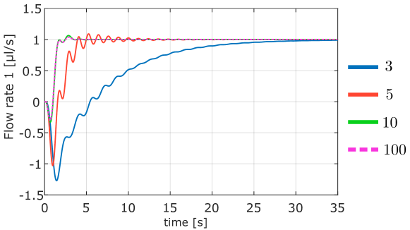
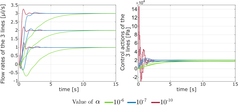
Figure 6: Simulated response of the flow rate $Q_{1}$ for $T=0.1$ s and different values of the horizon $N$. The setpoint is 1 $\mu$l/s and $\alpha=10^{-7}$.

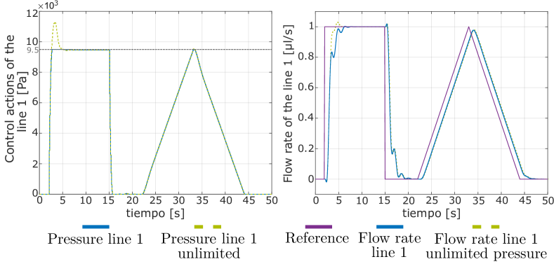
Figure 7: Simulated system response for $T=0.1$ s, horizon $N=10$, and different values of the parameter $\alpha$.

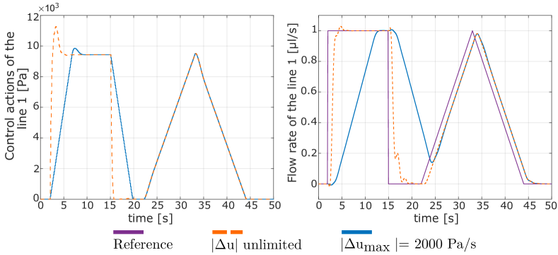
Figure 8: Simulation under constraints on the inputs.

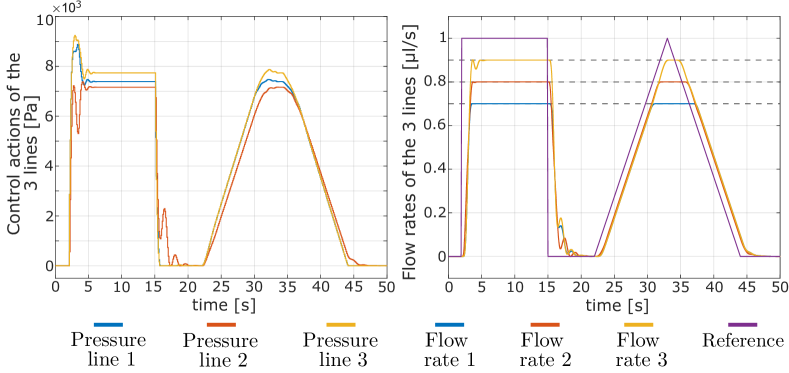
Figure 9: Simulation under constraints on the variation of the inputs.

Figure 10: Simulation under constraints on the flow rates.

VI Results of the complete implementation

After presenting the model, the observer, and the controller separately, this section reports the results obtained from tests conducted using the complete control system, both through simulation and in experiments carried out on the actual microfluidic system.

VI-A Validation by simulation

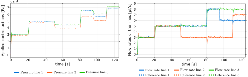
Figure 11: Simulation of the complete MPC system. Pressures (left) and flow rates (right) in response to stepped setpoints, different for each line.

Matlab-Simulink has been used to simulate the most realistic conditions. As described earlier, the plant has been modeled in continuous time and, accordingly, it is simulated using a precise numerical integration method that provides realistic results of the physical system response. Working in a simulation environment allows for measuring all state variables. It should be noted, however, that only the readings from the flow meters are used to provide feedback to the controller. These readings, to which simulated measurement noise can be added, serve as inputs to the observer, which estimates the rest of the state variables needed by the MPC algorithm. The controller is also provided with the desired values for the flow rates of the three lines. The controller performs the operations, and once the control action is calculated, it is applied to the plant, closing the loop. The simulations have been performed with a horizon $N=10$, a sampling period $T=0.1$ s, and values of $\alpha=10^{-7}$ and $\beta=10^{-4}$ for the controller and observer tuning parameters, respectively.

For the constraints to be imposed on the controller, the following considerations have been taken into account:

1. The maximum pressure of the controllers is limited by the pressure that the glass containers used in the experiments can withstand (150 000 Pa relative to atmospheric pressure). The minimum pressure is limited to atmospheric pressure.

2. The maximum rate of change has been determined based on the data provided from previous experiments. It is set at 100 000 Pa/s.

3. The only constraint on the flow rate in the lines entering the chip is that it must be positive, to prevent fluid from one line from entering another.

Fig. 11 shows the flow rates and pressures of the lines for a simulation in which stepped setpoints have been established, different for each of the flow rates. As in the observer validation, noise with variance $10^{-20}$ (m³/s)² has also been added to the three flow meters measurements. It can be seen that the system has a response time of approximately 1.8 seconds for lines 1 and 3, and 1.5 seconds for line 2. The results also show that the system correctly reaches the desired values with a small overshoot, which confirms that it works properly.

VI-B Validation on the real system

To conduct tests on the real system, the observer and controller code has been ported from Matlab to Python. The manufacturer of the devices used (Fluigent) provides a set of tools to easily communicate and control these devices from Python code, which is why this language has been chosen. In the following, some of the results obtained in the experiments are presented. The general constraints imposed are the same as in the simulations shown earlier, although for safety reasons the pressures on the real system have been kept below 100 000 Pa.

The parameters of the MPC controller are the same as those of the previous simulations. That is, $N=10$, $T=0.1$ s, and $\alpha=10^{-7}$. However, after some preliminary tests, it was observed that the real system exhibited more differences than expected from the model, especially in line 1, where an unexpected oscillatory dynamics was detected. Thus, to deal with this uncertainty, it was considered that the matrix $\mathbf{Q_{\scriptscriptstyle KF}}$ of the filter required some manual adjustment. The values of each of the submatrices finally used are as follows:

$$\mathbf{Q_{\scriptscriptstyle KF}}_{Q} =\mathrm{diag}\left(\left[50\;\;1\ \;\;10\;\;100\right]\right)\cdot 10^{-20},$$

$$\mathbf{Q_{\scriptscriptstyle KF}}_{P} =\mathrm{diag}\left(\left[10\;\;10\ \;\;10\;\;10\;\;1\;\;1\;\;1\;\;1\;\;1\right]\right)\cdot 10^{5},$$

where $\mathrm{diag}(\cdot)$ is an operator that constructs a diagonal matrix with the elements of the argument vector on the main diagonal and zeros in the remaining elements. The covariance of the measurement noise has been kept at the same value ($\mathbf{R_{\scriptscriptstyle KF}}=\mathbf{I}_{p}\cdot 10^{-20}$).

Fig. 12 shows the flow rates and pressures for the case already studied by simulation, with different stepped setpoints for each line. The results clearly show that the behavior of the middle line (line 2) is, as expected, different from the other two. In the flow rate plot of this case, as well as in those that will be presented later, it can be observed the previously mentioned oscillations in line 1 (in blue), which become more pronounced with higher flow rates. After several tests in the laboratory, it was concluded that this is due to unmodeled dynamics of this specific pressure regulator. There are other significant differences compared to the simulation, especially in the pressure plot, but it can still be seen that the proposed controller is able to achieve the desired flow rates in steady state. It can also be seen that disturbances appear in the lines when one of the others changes its value, but these are quickly corrected.

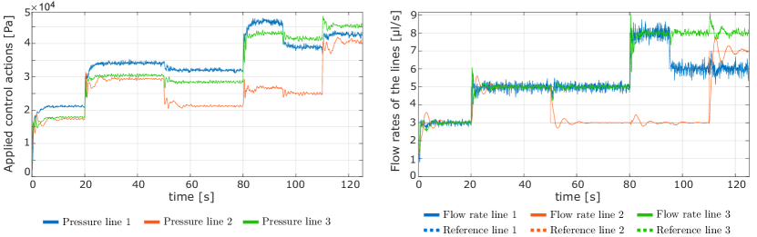
Figure 12: Real operation of the complete MPC system. Pressures (left) and flow rates (right) in response to stepped setpoints, different for each line.

In addition to this test, several other experiments have been conducted. For example, Fig. 14 shows the response of the system when the references are equal step functions for all three lines. Similar to the first case, it can be observed that the middle line takes longer to reach the reference than the other two. It is also noticeable that all three lines reach the steady state appropriately after the step functions. Some experiments have been done simply to illustrate compliance with the constraints imposed by the code. Fig. 14 shows, for example, one of the experiments conducted, in which a constraint of 60 000 Pa have been imposed on the maximum pressure in the pressure regulators. This pressure limit is established for verification purposes, as the normal operating limit is 150 000 Pa. It can be seen that the flow rates follow the reference value up to the moment when the pressure limitation prevents reaching higher flow rates.

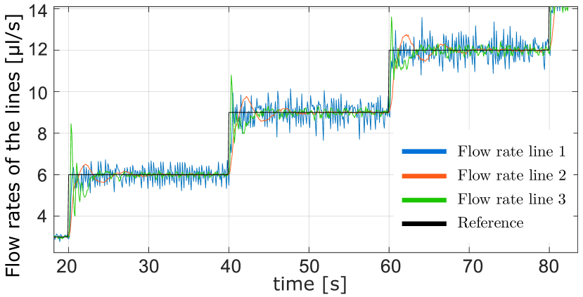
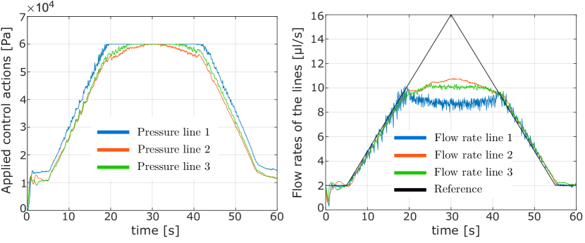
Figure 13: Real operation of the complete MPC system. Response of the flow rates to equal step setpoints for all three lines.

Figure 14: Real operation of the complete MPC control system. Pressures (left) and flow rates (right) in response to equal triangle setpoints for all three lines. A maximum value of 60 000 Pa has been imposed on the actions.

After the various experiments carried out on the real system, we can conclude that the designed controller allows to obtain flow rates at the chip inlet that adequately follow the desired reference values, while respecting the indicated constraints. The experiments also show that, although a simplification with a linear model has been used, the controller is capable of operating within the necessary working range, even in the presence of unexpected behaviors such as that of line 1. It has also been observed that modeling the dynamics of the pressure regulators is very important and that even two regulators of the same model and apparently identical can exhibit different behaviors.

VI-C Comparison with a classical controller

Finally, a comparison of the developed MPC controller with a classical controller has been performed by repeating the previous experiments but using an independent proportional-integral (PI) controller in parallel for each line. The possibility of including derivative action has been discarded due to the excessive presence of noise in the system. To make an objective comparison, the controllers have been optimized using the PID Tuner tool in Matlab, adjusting the proportional and integral gains, $k_{p}$ and $k_{i}$, to achieve the fastest response possible without overshoot. For lines 1 and 3, the gains are $k_{p}=5\cdot 10^{11}$ Pa/(m³/s) and $k_{i}=2.5\cdot 10^{12}$ Pa/m³; for line 2, $k_{p}=8.5\cdot 10^{10}$ Pa/(m³/s) and $k_{i}=1.5\cdot 10^{12}$ Pa/m³. The controllers include an anti-windup algorithm based on limiting the integral term.

In Figs. 15 and 17, the results obtained for the two stepped setpoint references are presented. It can be observed that the response of the system with the PI controllers is slower than that obtained in equivalent tests with the MPC, both in tracking the reference and in correcting one line when changes occur in the others. Specifically, the response time with the classical controller is between three and five times longer than with the MPC. Fig. 17 shows the response to the triangular reference signal, including the aforementioned limitation of 60 000 Pa on the maximum control action. It can be seen that the flow rates do not exactly follow the reference even before reaching saturation, contrary to what happened with the MPC (see Fig. 14). In this test, the MPC controller is also faster when the pressure saturation ends and returns to tracking the descending desired value. Finally, Table III shows the tracking errors for each of the flow rates for the three analyzed reference signals using each of the controllers. It can be seen that the MPC controller achieves lower errors in all cases.

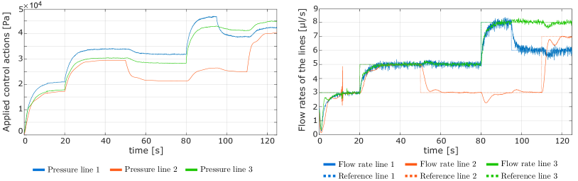
Figure 15: Real operation of the classical control system. Pressures (left) and flow rates (right) in response to different step references for each line.

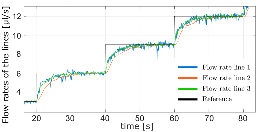
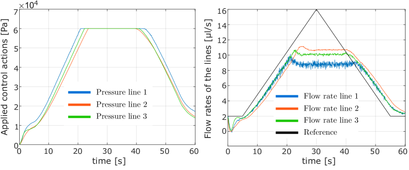
Figure 16: Real operation of the classical control system. Response of the flow rates to equal step setpoints for all three lines.

Figure 17: Real operation of the classical control system. Pressures (left) and flow rates (right) in response to equal triangle references for all three lines. A maximum value of 60 000 Pa has been imposed on the actions.

TABLE III: Comparison of results of MPC and classical controller. Root Mean Square Errors (RMSE) in $\mu$l/s.

Reference		RMSE $Q_{1}$	RMSE $Q_{2}$	RMSE $Q_{3}$
Different	MPC	0,325	0,384	0,262
steps	PI	0,490	0,705	0,425
Equal	MPC	0,566	0,475	0,411
steps	PI	0,723	0,980	0,681
Triangle	MPC	2,743	1,862	2,065
	PI	2,857	2,218	2,200

VII Conclusions

In this article, the design of a predictive controller for a microfluidic system has been described. Initially, it was necessary to develop a model to describe the fluid dynamics through the different channels and lines, as well as the behavior of the low-level sensors and regulators present in the system. Based on this, a state observer and the controller itself were designed, which were subsequently validated both by simulation and in the real system. The presented results show that the controller is effective in independently controlling the three flow rates circulating inside the microfluidic chip, even in the presence of noise and certain simplifications and uncertainties inherent in the model, and that the results improve upon what could be achieved with three independent classical controllers. It has also been observed that small variations in the operating conditions, e.g., the deformation of one of the conduits in the lines, can have a significant impact on the dynamics of the system. Thus, future research will focus on the development of online parameter estimation algorithms so that the control system can adapt to these changes.

References

- Bruus (2007) Bruus, H., 2007. Theoretical Microfluidics. Oxford Master Series in Physics. OUP Oxford.
-
Calle Chojeda et al. (2022)
Calle Chojeda, E., Oliden Semino, J., Ipanaqué Alama, W., 2022. Control de un sistema multivariable no lineal y en fase no mínima empleando un controlador predictivo neuronal. Revista Iberoamericana de Automática e Informática industrial 20 (1), 32–43.
DOI: 10.4995/riai.2022.17375 - Camacho and Bordons (2010) Camacho, E. F., Bordons, C., oct. 2010. Control Predictivo: Pasado, Presente y Futuro. Revista Iberoamericana de Automática e Informática industrial 1 (3), 5–28.
-
Clarke (1988)
Clarke, D., 1988. Application of generalized predictive control to industrial processes. IEEE Control Systems Magazine 8 (2), 49–55.
DOI: 10.1109/37.1874 -
Duinen et al. (2015)
Duinen, V. v., Trietsch, S. J., Joore, J., Vulto, P., Hankemeier, T., 2015. Microfluidic 3d cell culture: from tools to tissue models. Current Opinion in Biotechnology 35, 118–126.
DOI: 10.1016/j.copbio.2015.05.002 -
Gañán Calvo (1998)
Gañán Calvo, A. M., Jan 1998. Generation of steady liquid microthreads and micron-sized monodisperse sprays in gas streams. Phys. Rev. Lett. 80, 285–288.
DOI: 10.1103/PhysRevLett.80.285 -
Gallego Len et al. (2022)
Gallego Len, A. J., Sánchez del Pozo, A. J., F. Camacho, E., mar. 2022. Aplicaciones de control predictivo en plantas solares ccp. Revista Iberoamericana de Automática e Informática industrial 19 (3), 309–317.
DOI: 10.4995/riai.2022.16664 -
García-Camprubí et al. (2020)
García-Camprubí, M., Bengoechea-Cuadrado, C., Izquierdo, S., 2020. Virtual sensor development for continuous microfluidic processes. IEEE Trans. Ind. Informat. 16 (12), 7774–7781.
DOI: 10.1109/TII.2020.2972111 -
Ghadami et al. (2013)
Ghadami, M., Shagoshtasbi, H., Mahjoob, M., Lee, Y.-K., 2013. Comparative study of pid control and model predictive control for a microfluidic electroporation system. In: The 8th Annual IEEE International Conference on Nano/Micro Engineered and Molecular Systems. pp. 895–898.
DOI: 10.1109/NEMS.2013.6559867 -
Gómez et al. (2016)
Gómez, J. F., Barragán, A. J., Andújar, J. M., Reboso, J. A., Pérez, G. A., Méndez, J. A., Torres, J. M., Martínez, M. A., 2016. Control Predictivo basado en Modelo Borroso con EKF para el control de anestesia. In: XII Simposio CEA de Control Inteligente. pp. 7–11.
DOI: 10.13140/RG.2.2.21901.33764 -
Heo et al. (2016)
Heo, Y. J., Kang, J., Kim, M. J., Chung, W. K., 2016. Tuning-free controller to accurately regulate flow rates in a microfluidic network. Scientific Reports 6 (1), 23273.
DOI: 10.1038/srep23273 -
Kalman (1960)
Kalman, R. E., Mar. 1960. A New Approach to Linear Filtering and Prediction Problems. Journal of Basic Engineering 82 (1), 35–45.
DOI: 10.1115/1.3662552 -
Kim et al. (2013)
Kim, Y., LeDuc, P., Messner, W., Jan. 2013. Modeling and Control of a Nonlinear Mechanism for High Performance Microfluidic Systems. IEEE Trans. Control Syst. Technol. 21 (1), 203–211.
DOI: 10.1109/TCST.2011.2172445 -
Kuczenski et al. (2007)
Kuczenski, B., LeDuc, P. R., Messner, W. C., 2007. Pressure-driven spatiotemporal control of the laminar flow interface in a microfluidic network. Lab Chip 7, 647–649.
DOI: 10.1039/B617065J -
Li et al. (2022)
Li, Z., Hui, J., Yang, P., Mao, H., 2022. Microfluidic organ-on-a-chip system for disease modeling and drug development. Biosensors 12 (6).
DOI: 10.3390/bios12060370 -
Lucia et al. (2021)
Lucia, S., Navarro, D., Karg, B., Sarnago, H., Lucía, O., 2021. Deep learning-based model predictive control for resonant power converters. IEEE Trans. Ind. Informat. 17 (1), 409–420.
DOI: 10.1109/TII.2020.2969729 -
Maddala and Rengaswamy (2013)
Maddala, J., Rengaswamy, R., 2013. Droplet digital signal generation in microfluidic networks using model predictive control. Journal of Process Control 23 (2), 132–139, IFAC World Congress Special Issue.
DOI: 10.1016/j.jprocont.2012.08.014 -
Marchante et al. (2021)
Marchante, G., Acosta, A., González, A., Zamarreño, J., Álvarez, V., abr. 2021. Evaluación de restricciones de confort en controlador predictivo para la eficiencia energética. Revista Iberoamericana de Automática e Informática industrial 18 (2), 146–159.
DOI: 10.4995/riai.2020.13937 -
Martín-Banderas et al. (2005)
Martín-Banderas, L., Flores-Mosquera, M., Riesco-Chueca, P., Rodríguez-Gil, A., Cebolla, A., Chávez, S., Gañán Calvo, A. M., 2005. Flow focusing: A versatile technology to produce size-controlled and specific-morphology microparticles. Small 1 (7), 688–692.
DOI: 10.1002/smll.200500087 -
Miller et al. (2010)
Miller, E., Rotea, M., Rothstein, J. P., 2010. Microfluidic device incorporating closed loop feedback control for uniform and tunable production of micro-droplets. Lab Chip 10, 1293–1301.
DOI: 10.1039/B925497H -
Méndez Pérez et al. (2011)
Méndez Pérez, J. A., Torres, S., Reboso, J. A., Reboso, H., 2011. Estrategias de control en la práctica de anestesia. Revista Iberoamericana de Automática e Informática Industrial RIAI 8 (3), 241–249.
DOI: 10.1016/j.riai.2011.06.011 -
Ohno et al. (2008)
Ohno, K.-i., Tachikawa, K., Manz, A., 2008. Microfluidics: Applications for analytical purposes in chemistry and biochemistry. Electrophoresis 29 (22), 4443–4453.
DOI: 10.1002/elps.200800121 -
Rapp (2017)
Rapp, B. E., 2017. Chapter 17 - hydraulic resistance. In: Rapp, B. E. (Ed.), Microfluidics: Modelling, Mechanics and Mathematics. Micro and Nano Technologies. Elsevier, Oxford, pp. 351–370.
DOI: 10.1016/B978-1-4557-3141-1.50017-4 - Wang (2009) Wang, L., 2009. Model Predictive Control System Design and Implementation using MATLAB. Springer.
-
Wang et al. (2021)
Wang, Y., Wang, P., Qin, J., 2021. Microfluidic organs-on-a-chip for modeling human infectious diseases. Accounts of Chemical Research 54 (18), 3550–3562.
DOI: 10.1021/acs.accounts.1c00411 - Welch and Bishop (2006) Welch, G., Bishop, G., 2006. An Introduction to the Kalman Filter. Tech. rep., University of North Carolina at Chapel Hill.
- White (2008) White, F. M., 2008. Mecánica de fluidos, 6th Edition. McGraw-Hill.
- Çengel et al. (2018) Çengel, Y. A., Cimbala, J. M., Balderas Tapia, L., 2018. Mecánica de fluidos: fundamentos y aplicaciones., 4th Edition. McGraw-Hill Interamericana.