Cryptomite:
A versatile and user-friendly library of randomness extractors

Abstract

We present Cryptomite, a Python library of randomness extractor implementations. The library offers a range of two-source, seeded and deterministic randomness extractors, together with parameter calculation modules, making it easy to use and suitable for a variety of applications. We also present theoretical results, including new extractor constructions and improvements to existing extractor parameters. The extractor implementations are efficient in practice and tolerate input sizes of up to $2^{40}>10^{12}$ bits. They are also numerically precise (implementing convolutions using the Number Theoretic Transform to avoid floating point arithmetic), making them well suited to cryptography. The algorithms and parameter calculation are described in detail, including illustrative code examples and performance benchmarking.

1 Introduction

Informally, a randomness extractor is a function that outputs (near-)perfect randomness (in the sense that it is almost uniformly distributed) when processing an input that is ‘somewhat’ random (in the sense that it may be far from uniformly distributed). Randomness extractors play an essential role in many cryptographic applications, for example as exposure-resilient functions, to perform privacy amplification in quantum key distribution or to distil cryptographic randomness from the raw output of an entropy source. Beyond cryptography, randomness extractors are a useful tool for many tasks, including the de-randomisation of algorithms or constructing list-decodable error-correcting codes.

Despite their usefulness, a major difficulty is to select the appropriate randomness extractor and its parameters for the task at hand – and more generally, to design, optimise and implement the algorithm without significant expertise and time investment. To address this challenge, we have developed Cryptomite, a software library that offers state-of-the-art randomness extractors that are easy to use (see Section 4: ‘Cryptomite: Examples with Code’), efficient (see Section 2.3: ‘Performance’) and numerically precise (we use the number theoretic transform (NTT) [1] whenever implementing a suitable convolution to avoid floating point arithmetic).

The library contains extractors from existing work and our own constructions, along with several improvements to parameters and security proofs. With the library, we provide explanations, theorems and parameter derivation modules to assist the user and ensure that they make a good extractor choice for their application. Cryptomite is made available at https://github.com/CQCL/cryptomite under a public licence https://github.com/CQCL/cryptomite/blob/main/LICENSE for non-commercial use, and installable through pip, with command pip install cryptomite. In [2], we additionally show how to use the extractors in Cryptomite to post-process the output of several (quantum) random number generators and study their effect using intense statistical testing. We have also developed extractors that have: a) been further optimised for performance, b) been implemented on Field Programmable Gate Arrays (FPGA) and c) been implemented in constant time to avoid possible side-channel attacks. The details can be found in Section 2.4.

In the following, we give an overview of different types of randomness extractor (Section 1.1) and define our contributions (Section 1.2). Then, we present the Cryptomite library (Section 2) at a high level, describing each extractor and benchmarking the library’s performance, as well as providing a simple, visual guide to help a user in selecting the appropriate extractor. After that, we present the library in full detail (Section 3), where we give useful theorems and lemmas related to randomness extraction and explain how to calculate all relevant parameters. We finish with code examples (Section 4) on how to use Cryptomite extractors in experimental quantum key distribution and randomness generation, as well as the improvements that are achieved by using extractors of Cryptomite.

1.1 Randomness Extraction at a Glance

Randomness extractors transform strings of weakly random numbers (which we call the source or input), in the sense that their distribution has some min-entropy (the most conservative measure of a random variable’s unpredictability, see Definition 1), into (near-)perfect randomness, in the sense that the output’s distribution is (almost) indistinguishable from uniform (see Definitions 3 and 4), as quantified by an extractor error $\epsilon$. Some extractors require an additional independent string of (near-)perfect random numbers for this transformation, which we call the seed. Additionally, we also call the seed weak if it is not (near-)perfect but only has min-entropy.

In the manuscript, we use the notation $n_{1},n_{2}$ to denote the lengths (in bits) of the weakly random extractor input and the (weak) seed respectively. We use $k_{1},k_{2}$ (respectively) to denote their min-entropy, $m$ the extractor’s output length, $\epsilon$ the extractor error and $O(.)$ the asymptotic quantities related to the extractor algorithm, for example its computation time. The set-up and variables are illustrated in Figure 1.

Figure 1: An extractor processes a weak input of $n_{1}$ bits with min-entropy $k_{1}$ in order to produce an output of $m$ bits that is $\epsilon$-perfectly random. Seeded and two-source extractors additionally require a second bit string called the (weak) seed, of $n_{2}$ bits and min-entropy $k_{2}$ (with $k_{2}=n_{2}$ for seeded extractors).

At a high level, randomness extractors can be described by three classes:

• Deterministic Extractors are algorithms that process the weak input alone, without additional resources. Such extractors are able to extract from a subset of weakly random sources only, but require certain properties of the input distribution beyond just a min-entropy promise – for example that every bit is generated in an independent and identically distributed (IID) manner. A list of works detailing the different types of input which can be deterministically extracted from can be found in [3] (Subsection ‘Some related work on randomness extraction’).

• Seeded Extractors require an additional string of (near-)perfect randomness, called a seed, which is generated independently of the extractor weak input. By leveraging this additional independent randomness provided by the seed, they can extract from weak random inputs characterised by min-entropy only.

• Multi-Source Extractors, sometimes called blenders, are a generalisation of seeded extractors. They require one or multiple additional independent weak sources of randomness instead of a single (near-)perfect and independent one. In this work, the only multi-source extractors we consider are two-source, i.e. where the user has one addition weak input string only, which we call the weak seed.

When using randomness extraction algorithms in real-world protocols, the following features are crucial:

• Implementability and efficiency: Some randomness extractors only have non-constructive proofs and are therefore theoretical objects that can only be used to derive fundamental results. Moreover, although a randomness extractor may have an explicit construction, this does not always mean that the algorithm can be implemented with a computation time suitable for the application at hand. For example, taking directly the building blocks in [4] would lead to a computation time of $O(n_{1}^{4})$ (for $n_{1}\propto n_{2}$), which significantly limits the maximum input lengths that the implementation can handle. For most applications, a computation time of $O(n_{1}^{2})$ is a requirement, whilst many even require quasi-linear computation time $O(n_{1}\log(n_{1}))$.

• Additional resources: Seeded and two-source extractors require a seed, which is either near-perfect (seeded extractors) or weak (two-source extractor). In addition to the weakly random input to extract from, this oblige the user to have access to, or be able to generate, an independent (weak) seed, which can be difficult to justify (and often not even discussed). Because of this, it is important to minimise the resources required by the extractor, such as for example two-source extractors with low entropy requirements on the weak seed [5, 6] or extractors that suffice with a (near-)perfect seed that is only short [7, 8].

• Security options: Certain randomness extractor constructions have been shown to fail against a quantum adversary who can store (side-)information about weak sources in quantum states [9]. Because of this, it is important to have the option to choose extractors which are quantum-proof, for example in protocols such as quantum key distribution. Similarly, in certain protocols the adversary is able to perform actions that may correlate the input and the (weak) seed, therefore breaking the independence condition. This is the case for example in randomness amplification or could happen in quantum key distribution. Because of this, techniques exist that allow to weaken the independence condition [10, 11, 12].

• Entropy loss: Entropy loss is the difference between the min-entropy of the extractor input and the length of the extractor output. Some randomness extractors are able to extract with entropy loss that is only logarithmic in the inverse extractor error, which is the fundamental minimum [13], against both quantum and classical adversaries.

In Cryptomite, we implemented several randomness extractors that have a variety of the important features presented above. The extractors are efficient in practice, implemented with $O(n\log n)$ or $O(n^{2})$ time complexity, and have minimal or near-minimal entropy loss. They are able to extract from a wide array of different initial resources, allowing a user to pick the one most suited to their protocol. They also come with a wide range of options; such as whether to make them quantum-proof or secure when the extractor input and the (weak) seed are not fully independent. All extractors that we implement are strong, i.e. guarantee that the extractor output is statistically independent from one of its inputs, which for example allows for an increased output length by composing extractors together (see Section 3.2.5 and Definition 8 for the formal statement). They are information-theoretically secure, i.e. do not rely on computational assumption made on the adversary, and universally composable [14], allowing the extractor to be used securely as a part in a wider cryptographic protocol.

1.2 Our Contributions

The contributions of our work are:

1. We provide an efficient code implementation of a two-source $\mathsf{Dodis\hskip 2.84544ptet\hskip 2.84544ptal.}$ extractor, based on [15] and our previous work [16]. It is implemented in quasi-linear computation time $O(n\log n)$.

2. We present a new seeded extractor construction, which we call $\mathsf{Circulant}$, that can be understood as an extension of the $\mathsf{Dodis\hskip 2.84544ptet\hskip 2.84544ptal.}$ extractor. Beyond its simplicity, it is directly quantum-proof with the same error (and equivalently, the same output length), making it the best choice against quantum adversaries. It achieves the same entropy loss, quasi-linear efficiency and error as Toeplitz-based ones [18], whilst requiring a seed that is the same length as the weak input only – making it an excellent choice for tasks such as quantum key distribution.

3. We implement the $\mathsf{Toeplitz}$ extractor [18] efficiently (in $O(n\log(n))$) and a $\mathsf{Trevisan}$ extractor, based on [7] and [19], which tolerates the shortest seed lengths for sufficiently large input lengths but is less efficient ($O(n^{2}\log(\log(n)))$ complexity, making it impractical in many cases). We also provide an implementation of the deterministic $\mathsf{Von\hskip 2.84544ptNeumann}$ extractor in $O(n)$.

4. We implement the $\mathsf{Circulant}$, $\mathsf{Dodis\hskip 2.84544ptet\hskip 2.84544ptal.}$ and $\mathsf{Toeplitz}$ extractors using the number theoretic transform (NTT) which gives a throughput of approximately $1$Mbit/s for input sizes up to $5\times 10^{8}$ on a standard personal laptop (see Section 2.3). Using the NTT instead of the fast Fourier transform (FFT) avoids numerical imprecision (due to floating point arithmetic) which may be unsuitable for some applications, e.g. in cryptography, especially with large input lengths. The software is able to process input lengths of up to $2^{40}>10^{12}$ bits, which should be sufficient even for device independent protocols. When using input lengths below $2^{29}\approx 5\cdot 10^{8}$, the code uses a further optimised (smaller finite field for the) NTT to increase the throughput.

5. We collate (and sometimes improve) results from existing works into a single place, providing techniques to get the most (near-)perfect randomness in different adversarial models and experimental settings. For example, all our constructions can, as an option, extract under a weaker independence requirement on the weak seed (in the Markov model [11]) and we provide the associated parameters. Moreover, in the software we include ḟrom_params utility functions that calculates the output and input lengths in a number of settings.

To the best of our knowledge, related works have some, but not all, of the above features. In particular, $\mathsf{Circulant}$ is new to this work and no alternative work uses the NTT for extractor implementation. In terms of other works that implement randomness extractors, in [19], the authors provide a publicly available implementation of the $\mathsf{Trevisan}$ extractor only, whilst [20] gives a library of several randomness extractors (including $\mathsf{Von\hskip 2.84544ptNeumann}$, $\mathsf{Toeplitz}$ and $\mathsf{Trevisan}$), but does not implement the $\mathsf{Toeplitz}$ extractor with quasi-linear computation time, i.e. does not use the FFT or NTT. There are several publicly available implementations of the $\mathsf{Toeplitz}$ extractor alone, including [21, 22], none of which use the NTT to achieve both quasi-linear computation time and numerical precision. In [23] the authors discuss and implement the modified $\mathsf{Toeplitz}$ extractor, using the FFT and based on [8], which is a seeded extractor with similar parameters to $\mathsf{Circulant}$. We give a more detailed comparison between the constructions in Section 3.5. Other works collate existing results on extractors with the focus on aiding a user to implement and select them for their protocol, for example [24], however they do not provide the same level of flexibility or options as this work.

2 Overview of the Extractor Library

In this section, we present an overview of the Cryptomite extractors, an informal guide for selecting an appropriate extractor for an application, and performance benchmarking. Cryptomite is implemented in Python for usability and ease of installation, with performance-critical parts implemented in C++ called from Python.

2.1 Extractors of Cryptomite

The Cryptomite library contains

• The (new) $\mathsf{Circulant}$ seeded extractor. It requires a prime seed length of $n_{2}=n_{1}+1$ and outputs $m=\lfloor k_{1}-2\log_{2}(\frac{1}{\epsilon})\rfloor$ bits against both classical and quantum adversaries (called classical- and quantum-proof respectively). We offer different two-source extensions of the extractor, one of which has output length $m=\lfloor k_{1}+k_{2}-n_{2}-2\log_{2}(\frac{1}{\epsilon})\rfloor$ against an adversary with quantum side-information that is product on the two sources (see Section 3.2.1), and the other outputs roughly a fifth of that in the stronger Markov model of side-information [11], which can be informally understood as a model in which the inputs are independent only when conditioned on the adversary’s side-information (see Section 3.2.2).

• The $\mathsf{Dodis\hskip 2.84544ptet\hskip 2.84544ptal.}$ two-source extractor [15], with implementation based on [16]. It requires equal length inputs $n_{1}=n_{2}=n$, where $n$ is a prime with primitive root 2 and outputs $m=\lfloor k_{1}+k_{2}-n-2\log_{2}(\frac{1}{\epsilon})\rfloor$. Its quantum-proof version in the Markov model outputs $m=\lfloor\frac{1}{5}(k_{1}+k_{2}-n+8\log_{2}\epsilon+9-4\log_{2}(3))\rfloor$.

• The $\mathsf{Toeplitz}$ strong seeded extractors based on [18]. It requires a seed length of $n_{2}=n_{1}+m-1$ and outputs $m=\lfloor k_{1}-2\log_{2}(\frac{1}{\epsilon})\rfloor$, when classical-proof or quantum-proof with the same output length. We also offer two-source extensions of this extractor, whereby, the output becomes $m=\lfloor\frac{1}{2}(k_{1}+k_{2}-n_{1}+1-2\log_{2}(\frac{1}{\epsilon}))\rfloor$ against product quantum side-information and a third of that in the Markov model.

• The $\mathsf{Trevisan}$ seeded extractor [7], with implementation based on [19]. It requires a seed length of $n_{2}=O(\log(n_{1}))$ (see the exact statement of the seed length in Section 3.6) and outputs $m=\lfloor k_{1}-6-4\log_{2}(\frac{m}{\epsilon})\rfloor$ when classical-proof or quantum-proof with the same output length. As with $\mathsf{Circulant}$ and $\mathsf{Toeplitz}$, we offer two-source extensions, with the details deferred to Section 3.6.

• The $\mathsf{Von\hskip 2.84544ptNeumann}$ deterministic extractor [25]. Although this extractor does not require a seed, the weak input must have more structure than min-entropy. Additionally, this extractor incurs substantial entropy loss (see Section 3.7 for details). More precisely, it requires that the weak input forms an exchangeable sequence, e.g. a suitable weak input is one with IID bits.

Our implementations of the $\mathsf{Circulant}$, $\mathsf{Dodis\hskip 2.84544ptet\hskip 2.84544ptal.}$ and $\mathsf{Toeplitz}$ extractors all have $O(n_{1}\log(n_{1}))$ computation time and use the NTT. For these extractors, our code can tolerate input lengths $n_{1}\leq 2^{40}\approx 10^{12}$ bits – with an improved throughput version for any input lengths under $2^{29}$ (for more details, see Section 2.3). Our implementation of the $\mathsf{Von\hskip 2.84544ptNeumann}$ extractor has $O(n_{1})$ computational complexity and $\mathsf{Trevisan}$ has $O\left(n_{1}^{2}\log\log\left(\frac{n_{1}^{2}}{\epsilon}\right)\right)$. Again, all two-source and seeded extractors mentioned above are strong (see Definition 8) with the same error and output length.

2.2 A Simple User’s Guide

To help using Cryptomite, Figure 2 presents a flowchart which assists a user on deciding which extractor to use for their application and Figure 3 summarises the achievable parameters. The flowchart is somewhat informal and one can obtain small improvements by analysing each extractor individually (for example, finding a slightly longer output length or shorter seed size). The objective is to give a simple yet good choice for any application, in a clear and easy to follow diagram. In this guide, the user begins with some extractor input of length $n_{1}$ and min-entropy $k_{1}$ (Definition 1).

Figure 2: This flow chart shows the simplest way to get (approximately) the most output randomness from an input string of min-entropy $k_{1}$ and size $n_{1}$, whilst minimising the other resources (seed size and computation time). Small improvements can be obtained by considering Figure 3 below. In the left branch, the weak input bits need to form an exchangeable sequence, for which IID bits are a particular case.

Figure 3: A summary of the parameters achievable by the different randomness extractors in Cryptomite. For seeded extractors, one uses that $k_{2}=n_{2}$ and all logarithms are in base 2. $\mathbb{P}$ is the set of prime numbers, and $\mathbb{N}_{A}$ the set of prime numbers with 2 as a primitive root (see Section 3.4). The parameters for classical side-information in the Markov model are not included, but can be computed from Theorem 3. The $\mathsf{Trevisan}$ output length against quantum side-information with product sources is only known in the seeded case ($k_{2}=n_{2}$), whilst we could not find results with weak seeds ($k_{2}<n_{2}$) for both $\mathsf{Trevisan}$ and $\mathsf{Dodis\hskip 2.84544ptet\hskip 2.84544ptal.}$ (although one can use the values for the Markov model). Finally, the output length for $\mathsf{Von\hskip 2.84544ptNeumann}$ is probabilistic and given in the case of IID bits as input (denoted $\approx^{IID}$).

2.3 Performance

To demonstrate the capabilities of Cryptomite, we perform some benchmarking of our constructions on a Apple M2 Max with 64GB RAM processor. The throughput (output bits per second) of the extractors of Cryptomite are shown in Figure 4. It is calculated by averaging the run-time over 10 trials, for each input length, for input lengths up to $5\times 10^{8}$. Note that when the input length is below $2^{29}>5\times 10^{8}$ bits, the convolution based extractors ($\mathsf{Circulant}$, $\mathsf{Dodis\hskip 2.84544ptet\hskip 2.84544ptal.}$ and $\mathsf{Toeplitz}$) perform operations over a finite field defined by the prime $p=3\times 2^{30}+1$. For input lengths above $2^{29}$ and up to $2^{40}$, the operations must be implemented in a larger finite field, and we use the prime $p^{\prime}=9\times 2^{42}+1$ (which we call bigNTT). This change comes at the cost of approximately a 3-4$\times$ reduction in throughput.

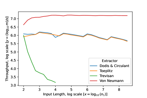
Figure 4: A plot displaying the throughput of our extractor algorithms as a function of the input size ($n_{1}$) for each extractor of Cryptomite, in logarithmic scale. The throughput is calculated by fixing the input min-entropy to $k_{1}=\frac{n_{1}}{2}$ and calculating the maximum output length according to Figure 3. The run-time is independent of the output length ($m$) for the $\mathsf{Circulant}$, $\mathsf{Dodis\hskip 2.84544ptet\hskip 2.84544ptal.}$ and $\mathsf{Toeplitz}$ extractors due to the NTT implementation step which handles a square matrix of size $n_{1}\times n_{1}$ before outputting the first $m$ bits. This means that, for those extractors, the throughput could be doubled if the input had min-entropy $k_{1}\sim n_{1}$. The necessary seed size for each extractor is given in Section 3.

Some observations are:

• The $\mathsf{Circulant}$, $\mathsf{Dodis\hskip 2.84544ptet\hskip 2.84544ptal.}$ and $\mathsf{Toeplitz}$ extractors are able to output at speeds of up to $\approx 1$Mbit/s, even for large input lengths. The slight gradual decline in the larger input lengths is expected to be due to CPU characteristics such as cache hit rate and branch prediction.

• The $\mathsf{Trevisan}$ extractor can generate output at speeds comparable to the $\mathsf{Circulant}$, $\mathsf{Dodis\hskip 2.84544ptet\hskip 2.84544ptal.}$ and $\mathsf{Toeplitz}$ extractors only when the input or output size is (very) short. It can not generate a non-trivial throughput for input lengths greater than $n_{1}\approx 10^{4}$.

• The throughput is lower for short input lengths of the $\mathsf{Von\hskip 2.84544ptNeumann}$ extractor due to some constant time overhead.

2.4 Further Optimised Extractor Implementations

We have also developed enhanced versions of our extractor implementations, namely:

• Improved throughput: for our $\mathsf{Circulant}$ and $\mathsf{Dodis\hskip 2.84544ptet\hskip 2.84544ptal.}$ extractors, the throughput is in general between $7-10\times$ the versions in Cryptomite.

• Constant-time implementation: in cryptography, variable run-time opens the door for side-channel attacks, so we have implemented constant-time versions of our extractors.

• FPGA implementations: we have field-programmable gate array (FPGA) implementations of our $\mathsf{Circulant}$ and $\mathsf{Dodis\hskip 2.84544ptet\hskip 2.84544ptal.}$ extractor.

• Optimised short input implementation: we have versions of $\mathsf{Circulant}$ and $\mathsf{Dodis\hskip 2.84544ptet\hskip 2.84544ptal.}$ that are extensively optimised for small input lengths, improving its throughput further (up to 20$\times$).

These further optimised constructions are only available on demand, contact qcrypto@quantinuum.com.

3 Library in Detail

In this section, we define the extractors in Cryptomite concretely, giving the implementation details and parameter calculations. First, we introduce the notation and relevant definitions that we use for the remainder of the manuscript and provide some useful lemmas and theorems related to randomness extraction (which may be of independent interest). The reader who is only interested in using our extractors can skip the preliminaries and go straight to the section for their extractor of choice and take the parameters directly, or use the repository documentation and parameter calculation modules that we make available.

3.1 Preliminaries

We denote random variables using upper case, e.g. $X$, which take values $x$ in some finite alphabet with probability $\mathrm{Pr}(X=x)=p_{X}(x)$, and for some random variable $E$ taking values $e$, we write the conditional and joint probabilities as $\mathrm{Pr}(X=x|E=e)=p_{X|E=e}(x)$ and $\mathrm{Pr}(X=x,E=e)=p_{X,E}(x,e)$ respectively. We call the probability $p_{\mathrm{guess}}(X)=\max_{x}p_{X}(x)$ the (maximum) guessing probability and the (maximum) conditional guessing probability $p_{\mathrm{guess}}(X|E)=\max_{x,e}p_{X|E=e}(x)$ (for more detailed discussions and explanations, see [26]). In this work, we focus on the case that the extractor inputs are bit strings, e.g. $X\in\{0,1\}^{n}$ is a random variable of $n$ bits, and $X=x$ is its realisation. Since the realisations $x$ are bit strings, we denote the individual bits with a subscript, e.g. $x=x_{0},\ldots,x_{n-1}$ where $x_{i}\in\{0,1\}$ for all $i\in 0,\ldots,n-1$. Let $[,]$ denote the concatenation of random variables, for example, if $X\in\{0,1\}^{n_{1}}$ and $Y\in\{0,1\}^{n_{2}}$, then $[X,Y]\in\{0,1\}^{n_{1}+n_{2}}$. Throughout the manuscript, all logarithms are taken in base 2 and all operations are performed modulo 2, unless explicitly stated otherwise.

The concept of weak randomness, as we are interested in, is captured by the (conditional) min-entropy, which can be interpreted as the minimum amount of random bits in $X$, conditioned on the side information $E$ that a hypothetical adversary might possess.

Definition 1 (Conditional min-entropy).

The (conditional) min-entropy $k$ of a bit string $X\in\{0,1\}^{n}$, denoted $\mathrm{H}_{\infty}(X|E)$, is defined as

$$k=\mathrm{H}_{\infty}(X|E)=-\log_{2}\left(p_{\mathrm{guess}}(X|E)\right)$$ (1)

where $E$ is a random variable that contains any additional (or side-) information a hypothetical adversary may have to help predict $X$. For a given bit string, we call its total (conditional) min-entropy divided by its length the min-entropy rate $\alpha=\frac{k}{n}$.

In order for randomness extractors to be useful in a cryptographic application, their output must satisfy a universally composable [14] security condition. This condition is best understood by imagining a hypothetical game in which a computationally unbounded adversary is given both the real output of the extractor and the output of an ideal random source. The adversary wins the game if they are able to distinguish between these two bit strings, i.e. guess which of the bit strings came from the extractor versus from the ideal random source. A trivial adversarial strategy is to guess at random, giving a success probability of $1/2$ and, for a secure protocol, we ask that a computationally unbounded adversary can not distinguish the bit strings with success probability greater than $\frac{1}{2}+p_{\textrm{dist}}$, for $p_{\textrm{dist}}\ll 1$. In other words, the best strategy, even for a very powerful adversary, is not much better than the trivial one. This definition of security is formalised using distance measures as follows.

Definition 2 (Statistical distance).

The statistical distance $\Delta$ between two random variables $X$ and $Y$, with $X,Y\in\{0,1\}^{n}$, conditioned on information $E$ (a random variable of arbitrary dimension), is given by

$$\Delta\!\left(X,Y|E\right) =\frac{1}{2}\max_{e}\sum\limits_{x}\lvert p_{X|E=e}(x)-p_{Y|E=e}(x)\rvert.$$ (2)

If $X$ and $Y$ satisfy $\Delta\!\left(X,Y|E\right)\leq\epsilon$ , we then say that they are $\epsilon$-close (given $E$), which implies that they can be distinguished with advantage $p_{\textrm{dist}}\leq\frac{\epsilon}{2}$. This allows us to quantify how close a distribution is to uniform, which gives rise to our term (near-) perfect randomness, where near- is quantified by the distance bound.

Definition 3 (Classical-proof (near-)perfect randomness).

The random variable $Z\in\{0,1\}^{m}$ is (near-)perfectly random (given $E$), quantified by some value $\epsilon\in(0,1)$, if it is $\epsilon$-close to the uniform distribution $\mathrm{U}_{m}$ over $\{0,1\}^{m}$, i.e.

$$\Delta\!\left(Z,\mathrm{U}_{m}|E\right)\leq\epsilon.$$ (3)

In our context, $\epsilon$ is called the extractor error. In practice, $\epsilon$ is a fixed security parameter, for example, enforcing that $\epsilon=2^{-32}$.

We call the definitions that we have given so far classical-proof, in the sense that the adversary’s information is classical (a random variable $E$). When the adversary has access to quantum states to store information, there are situations in which security cannot be guaranteed with Definition 3 alone (see [9] for a concrete example and [27] for a general discussion). Because of this, in what follows we generalise our definitions to the quantum case and say that these are secure against quantum adversaries, or quantum-proof.

A random variable $X\in\{0,1\}^{n}$ with $p_{X}(x)$ can be written as a quantum state living in the Hilbert space $\mathcal{X}$ as $\rho_{\mathcal{X}}=\sum_{x\in\{0,1\}^{n}}p_{X}(x)\ket{x}\!\!\bra{x}$, where the vectors $\{\ket{x}\}_{x}$ form an orthonormal basis. Considering quantum adversaries (with quantum side-information), the classical variable $X$ can be considered part of a composite system potentially correlating it with the adversary in a Hilbert space $\mathcal{X}\otimes\mathcal{E}$, which can be written as the classical-quantum state

$$\rho_{\mathcal{X}\mathcal{E}}=\sum_{x\in\{0,1\}^{n}}p_{X}(x)\ket{x}\!\!\bra{x}_{\mathcal{X}}\otimes\rho_{\mathcal{E}|x}.$$ (4)

In Equation 4 the adversary’s part of the system is the state $\rho_{\mathcal{E}|x}$, which is conditioned on the realisation $X=x$. In the quantum case, the conditional min-entropy (given $\mathcal{E}$) of the classical variable $X$ is $\mathrm{H}_{\infty}(X|\mathcal{E})=-\log_{2}(p_{\mathrm{guess}}(X|\mathcal{E}))$, where $p_{guess}(X|\mathcal{E})=\max_{\{M_{x}\}_{x}}\sum_{x}\Tr(M_{x}\rho_{\mathcal{E}|x})$ is the adversary’s maximum guessing probability to guess $X$, given all measurement strategies $M_{x}$ on their system $\rho_{\mathcal{E}|x}$. For a general discussions on min-entropy in the presence of quantum adversaries, see [28].

Similarly to the classical case, an extractor ideally outputs the classical-quantum state $\mathrm{u}_{\mathcal{Z}}\otimes\rho_{\mathcal{E}}$, where $\mathrm{u}_{\mathcal{Z}}$ is the maximally mixed state and independent of the state of the adversary

$$\mathrm{u}_{\mathcal{Z}}\otimes\rho_{\mathcal{E}}=2^{-m}\!\!\!\!\sum_{{z}\in\{0,1\}^{m}}\!\!\ket{z}\!\!\bra{z}_{\mathcal{Z}}\otimes\rho_{\mathcal{E}}.$$ (5)

Analogously to the classical case, the quantum-proof security criterion is that the randomness extraction process produces a real state (Equation 4 with $Z$ as the classical subsystem) that is essentially indistinguishable from the ideal state Equation 5. Intuitively, such an ideal state promises that the output $\mathbf{z}$ remains unpredictable for all adversarial strategies using their state $\rho_{\mathcal{E}|z}$. This criterion for security against an adversary who has access to quantum side information is formalised in the following definition.

Definition 4 (Quantum-proof (near-)perfect randomness).

The extractor output $Z\in\{0,1\}^{m}$ is quantum-proof $\epsilon$-perfectly random if

$$\Delta_{Q}\!(Z,\mathrm{U}_{m}|\mathcal{E})=\frac{1}{2}\|\rho_{\mathcal{Z}\mathcal{E}}-\mathrm{u}_{\mathcal{Z}}\otimes\rho_{\mathcal{E}}\|_{1}\leq\epsilon$$ (6)

where $\|\cdot\|_{1}$ denotes the trace norm, defined as $\|\sigma\|_{1}=\mathrm{Tr}(\sqrt{\sigma^{\dagger}\sigma})$. We use the subscript $Q$ and the conditioning on the quantum state $\mathcal{E}$ to mark the distinction with the classical version $\Delta\!(Z,\mathrm{U}_{m}|E)$.

For a discussion on why this is the correct measure against quantum adversaries, see [17] ‘Section 2’.

We can now define what deterministic, seeded and two-source extractors are at the function level. For simplicity of notation, we omit the conditioning on the side information $E$ (or $\mathcal{E}$), for example, writing $\mathrm{H}_{\infty}(X)$ instead of $\mathrm{H}_{\infty}(X|E)$.

Definition 5 (Deterministic randomness extractor).

A $(\epsilon,n,m)$-deterministic extractor is a function

$$\mathsf{Ext_{d}}:\{0,1\}^{n}\rightarrow\{0,1\}^{m}$$ (7)

that maps a random bit string $X\in\{0,1\}^{n}$ with some specific properties, to a new variable $Z=\mathsf{Ext_{d}}(X)$ that is (optionally quantum-proof) $\epsilon$-perfectly random, see Definition 3 (optionally Definition 4).

Definition 6 (Two-source randomness extractor).

Given two independent random variables $X\in\{0,1\}^{n_{1}}$ and $Y\in\{0,1\}^{n_{2}}$, with min-entropy $\mathrm{H}_{\infty}(X)\geq k_{1}$ and $\mathrm{H}_{\infty}(Y)\geq k_{2}$ respectively, a $(k_{1},k_{2},\epsilon,n_{1},n_{2},m)$-two-source randomness extractor is a function

$$\mathsf{Ext_{2}}:\{0,1\}^{n_{1}}\times\{0,1\}^{n_{2}}\rightarrow\{0,1\}^{m}$$ (8)

where $\mathsf{Ext_{2}}(X,Y)$ is $\epsilon$-perfectly random, see Definition 3 (optionally Definition 4).

We discuss the role of side-information for two-source extractors in Section 3.2. When discussing two-source extractors, we will refer to the input $X$ as the extractor input and $Y$ as the weak seed. In the case that $Y$ is already near-perfectly random, we will simply call it the seed.

Definition 7 (Seeded randomness extractor).

A seeded extractor is a special case $(k_{1},k_{2}=n_{2},\epsilon,n_{1},n_{2},m)$-two-source randomness extractor, where $k_{2}=n_{2}$.

We have mentioned that our extractors are strong, and now we define this property

Definition 8 (Strong randomness extractor).

A $(k_{1},k_{2},\epsilon,n_{1},n_{2},m)$-randomness extractor $\mathsf{Ext}:X\in\{0,1\}^{n_{1}}\times Y\in\{0,1\}^{n_{2}}\to\{0,1\}^{m}$ is strong in the input $Y$ if,

$$\Delta\!([\mathbf{\mathsf{Ext}}(X,Y),Y],[\mathrm{U}_{\mathrm{m}},Y])\leq\epsilon$$ (9)

or quantum-proof strong in the input $Y$ if

$$\Delta_{Q}\!([\mathbf{\mathsf{Ext}}(X,Y),Y],[\mathrm{U}_{\mathrm{m}},Y])\leq\epsilon,$$ (10)

where $\mathrm{U}_{\mathrm{m}}$ denotes the uniform distribution over $m$ bits. Informally, this can be understood as the property that the extractor output bits are near-perfect, even conditioned on the input $Y$.

By convention, we will always assume that the extractor is strong in the (weak) seed, although the role of the input sources can usually be exchanged for two-source extractors. All extractors presented in this work are strong with the same error and output length. Having this additional property leads to some useful consequences:

1. $Y$ may become known to the adversary without compromising the security of the extractor output, i.e. the extractor output remains $\epsilon$-perfectly random.

2. $Y$ can be re-used in multiple rounds of randomness extraction (with additive error $\epsilon$), under the assumption that each of the subsequent weak extractor inputs, say $X_{2},X_{3},\ldots$, are also independent of $Y$ (see Theorem 5).

3. If $Y$ is near-perfectly random (the case of seeded extractors), it can be concatenated with the extractor output to increase the output length. If $Y$ only has min-entropy, it can be reused as the extractor input to another seeded extractor taking the output of the two-source extractor as seed. This alows to extract roughly all the min-entropy $\mathrm{H}_{\infty}(Y)$ (see Section 3.2.5).

Option 2 is compatible with options 1 and 3 (they can be achieved simultaneously), however option 3 is not compatible with 1.

3.2 Useful Theorems and Results

Next, we reproduce and extend results from other works, which provides flexibility in the extractors’ use. First, we see how to account for side-information with two-source extractors, where both sources might be correlated to the adversary’s information. Second, we explain how to use extractors with a bound on the smooth min-entropy only and how to account for near-perfect seeds (which can also be reused in multiple extraction rounds). Third, we see how to generically extend a seeded extractor to a two-source one, as well as how to manipulate the input lengths to construct a family of extractors that can be optimised over. Finally, as mentioned above, we explain how one can concatenate two-source and seeded extractors in order to obtain more advantageous constructions.

3.2.1 Two-source extractors in the product sources model

Seeded randomness extractors are well studied in the presence of side-information and quantum-proof constructions with minimal (or near minimal) entropy loss are known to exist [31, 32, 33, 8], where the weak input to the extractor is in a classical-quantum state, see Equation 4. Multi-source extractors, including two-source extractors require more care, as the adversary might now posses side-information about both sources (for example potentially correlating the sources).

Hayashi and Tsurumaru [8] showed that any strong classical-proof seeded extractor has a two-source extension, whereby the extractor can be used with a non-uniform seed at the cost of a larger error or shorter output length. Moreover, they give an improved extension when the extractor is based on two-universal families of hash functions.

Theorem 1 (Classical-proof two-source extension, Theorem 6 and 7 in [8]).

Any strong classical-proof (or quantum-proof) $(k_{1},n_{2},\epsilon,n_{1},n_{2},m)$-seeded extractor is a strong classical-proof (or quantum-proof) $(k_{1},k_{2},2^{n_{2}-k_{2}}\epsilon,n_{1},n_{2},m)$-two-source extractor, strong in the (now) weak seed. If the extractor is constructed from a two-universal family of hash functions, it is a strong classical-proof (or quantum-proof) $(k_{1},k_{2},2^{(n_{2}-k_{2})/2}\epsilon,n_{1},n_{2},m)$-two-source extractor.

The quantum-proof claim in Theorem 1 does not directly cover quantum side-information about the (now) weak seed, only on the weak input, and still demands that the weak seed and weak input are independent. Using the proof techniques of [36] (‘Proof of proposition 1’) this can be directly generalised to the case that an adversary has quantum side-information about both the input and the weak seed, but with the constraint that, for extractors based on two-universal hash families, this side-information is in product form. More concretely, this is the case when the input and the now weak seed form a so-called classical-classical quantum-quantum state, whereby the combined two-universal hashing based extractor input (for the input and (weak) seed given by Equation 4) takes the form

$$\rho_{XY\mathcal{E}_{1}\mathcal{E}_{2}}=\rho_{X\mathcal{E}_{1}}\otimes\rho_{Y\mathcal{E}_{2}}.$$ (11)

This model for quantum-proof extractors is the product sources model.

Theorem 2 (Quantum-proof two-source extension in the product sources model, Theorem 1 with Proposition 1 in [36]).

Any strong quantum-proof $(k_{1},n_{2},\epsilon,n_{1},n_{2},m)$-seeded extractor based on two-universal hash families is a strong quantum-proof $(k_{1},k_{2},2^{(n_{2}-k_{2})/2}\epsilon,n_{1},n_{2},m)$-two-source extractor in the product sources model.

Proof.

The proof of this follows directly from [36] ‘Proof of proposition 1’ by noticing that $n-1$ can be generically replaced with $n_{2}$, the length of the (weak) seed and that their bound on $(*)$ (as appearing in the text) is found by bounding the collision entropy of the seeded version of the extractor, which holds for all extractors based off two-universal families of hash functions. ∎

3.2.2 Two-source extractors in the Markov model

Two-source extractors can also be made secure in the so-called Markov model [11], which considers evens stronger adversaries than in the product sources model. Instead of requiring the standard independence relation between the input and weak seed, i.e. that the mutual information $\mathrm{I}(X:Y)=0$, one can use randomness extractors in the presence of side-information that correlates the inputs by taking a penalty on the error or output length. The authors prove their results in the general cases of multi-source extractors, so we restate their theorems in the special case of two-source extractors.

In the case of classical side-information $E$, with $\mathrm{I}(X:Y|E)=0$ instead of $\mathrm{I}(X:Y)=0$ and with conditional min-entropy’s $\mathrm{H}_{\infty}(X|E)\geq k_{1}$ and $\mathrm{H}_{\infty}(Y|E)\geq k_{2}$;

Theorem 3 (Classical-proof in the Markov model, Theorem 1 in [11]).

Any $(k_{1},k_{2},\epsilon,n_{1},n_{2},m)$ (strong) two-source extractor is a $(k_{1}-\log_{2}(\frac{1}{\epsilon}),k_{2}-\log_{2}(\frac{1}{\epsilon}),3\epsilon,n_{1},n_{2},m)$ classical-proof randomness extractor in the Markov model.

In the quantum case (where the quantum side-information of the adversary is now a quantum system $\mathcal{E}$) one requires $\mathrm{I}(X:Y|\mathcal{E})=0$ instead of $\mathrm{I}(X:Y)=0$ and that both sources have conditional min-entropy, i.e. $\mathrm{H}_{\infty}(X|\mathcal{E})\geq k_{1}$ and $\mathrm{H}_{\infty}(Y|\mathcal{E})\geq k_{2}$.

Theorem 4 (Quantum-proof in the Markov model, Theorem 2 in [11]).

Any $(k_{1},k_{2},\epsilon,n_{1},n_{2},m)$ (strong) two-source extractor is a $(k_{1}-\log_{2}(\frac{1}{\epsilon}),k_{2}-\log_{2}(\frac{1}{\epsilon}),\sqrt{3\epsilon 2^{m-2}},n_{1},n_{2},m)$ quantum-proof randomness extractor in the Markov model.

The Markov model is particularly relevant in protocols for randomness amplification [37, 16] and in quantum key distribution (QKD). Other works have considered different forms of quantum side-information, for example, where the adversary is allowed specific operations in order to build the side-information $\mathcal{E}$ [38] or when there is a bound on the dimension of the adversary’s side-information [39]. However, most of these other forms of side-information can be viewed as a particular case of the Markov one, making it a useful generic extension to use – see the discussion in [11] (Section 1.2: ‘Related work’). In the classical case, [10] explores what happens to the security of two-source extractors when the extractor input and the weak seed can be correlated in some specific models, for example, when they have bounded mutual information $I(X:Y)\leq t$, for some constant $t$.

3.2.3 Working with near-perfect seeds and smooth min-entropy bounds

Seeded randomness extraction can be performed using seeds that are near-perfectly random only (instead of perfectly random), making it more practical. Strong seeded extractors allow the seed to be reused multiple times, and so we give a theorem that accounts for this seed reuse and we discuss this more in Section 3.2.5.

Theorem 5.

[Extractors with (near-)perfect seeds, Appendix A in [40]] Given an $\epsilon_{s}$-perfect seed $Y$, which is used to extract $t$ times from a weak source with $X_{i}$ for $i=1,...,t$ such that $\mathrm{H}_{\infty}(X_{i}|X_{i-1},...,X_{1})\geq k$ for all $i$ using a strong $(k,n_{2},\epsilon,n_{1},n_{2},m)$-seeded extractor $\mathsf{Ext_{s}}(X,Y)$ each time, the concatenated output $[\mathsf{Ext_{s}}(X_{1},Y),...,\mathsf{Ext_{s}}(X_{t},Y)]$ is $\epsilon_{t}$-perfect with

$$\epsilon_{t}\leq t\cdot\epsilon+\epsilon_{s}.$$ (12)

Similarly, in practice, often only a bound on the smooth min-entropy can be obtained, for example when using the (generalised) entropy accumulation theorem [41, 42, 43, 44] or probability estimation factors [45, 46, 47]. We give two theorems that allow for seeded and two-source extractors to function with inputs that have a promise on their smooth min-entropy.

Theorem 6 (Seeded extraction with smooth min-entropy, e.g. Corollary 7.8 in [48]).

Given a (strong) quantum-proof seeded extractor $(k,n_{2},\epsilon,n_{1},n_{2},m)$, one can use a weak input $X$ with smooth min-entropy $\mathrm{H}_{\infty}^{\delta}(X|\mathcal{E})\geq k$ at the cost of an additive error $\epsilon+\delta$, i.e. $(k,n_{2},\epsilon+\delta,n_{1},n_{2},m)$.

Theorem 7 (Two-source extraction with smooth min-entropy, Lemma 17 in [44]).

Given a (strong) quantum-proof two-source extractor $(k_{1}-\log_{2}(1/\epsilon_{1})-1,k_{2}-\log_{2}(1/\epsilon_{2})-1,\epsilon,n_{1},n_{2},m)$ in the Markov model (see Section 3.2.2), one can use weak inputs $X$ and $Y$ satisfying $\mathrm{I}(X:Y|\mathcal{E})=0$ with smooth min-entropy’s $\mathrm{H}_{\infty}^{\delta_{1}}(X|\mathcal{E})\geq k^{\prime}_{1}$ and $\mathrm{H}_{\infty}^{\delta_{2}}(Y|\mathcal{E})\geq k^{\prime}_{2}$ giving a

$$(k^{\prime}_{1}-\log_{2}(\frac{1}{\epsilon_{1}}),k^{\prime}_{2}-\log_{2}(\frac{1}{\epsilon_{2}}),2\epsilon+6(\delta_{1}+\delta_{2})+2(\epsilon_{1}+\epsilon_{2}),n_{1},n_{2},m)\mathrm{-extractor}$$ (13)

This result also applies to classical-proof extractors and, because of the generality of the Markov model, to many other forms of (quantum) side-information [11].

3.2.4 Extractor extensions to more settings

As some of our extractors require specific input lengths (for example, that the input length must be prime), we give some results that give flexibility to increase or decrease the length of the extractor input, which later allow us to optimise the output length. First, we show that any two-source extractor is a seeded extractor, using only a short seed padded with fixed bits (i.e. these additional bits do not have any entropy).

Theorem 8 (Short seeded extractors from two-source ones).

A $(k_{1},k_{2},\epsilon,n_{1},n_{2},m)$-two-source randomness extractor $\mathsf{Ext_{2}}$ is also a $(k_{1},k_{2},\epsilon,n_{1},k_{2},m)$-seeded randomness extractor $\mathsf{Ext_{s}}$, where $\mathsf{Ext_{s}}(X,Y)=\mathsf{Ext_{2}}(X,[Y,c])$ and $[Y,c]$ is the seed $Y\in\{0,1\}^{\lfloor k_{2}\rfloor}$ concatenated with a fixed string $c\in\{0,1\}^{n_{2}-\lfloor k_{2}\rfloor}$, e.g. $c=\{0\}^{n_{2}-\lfloor k_{2}\rfloor}$.

Proof.

Let $Y\in\{0,1\}^{\lfloor k_{2}\rfloor}$ be the seed of the extractor $\mathsf{Ext_{s}}$, i.e. $\mathrm{H}_{\infty}(Y)=\lfloor k_{2}\rfloor$, and $c\in\{0,1\}^{n_{2}-\lfloor k_{2}\rfloor}$ a constant (or fixed) string, i.e. (informally) $\mathrm{H}_{\infty}(c)=0$. Then $Y^{\prime}\equiv[Y,c]$ has $\mathrm{H}_{\infty}(Y^{\prime})=\mathrm{H}_{\infty}([Y,c])=\mathrm{H}_{\infty}(Y)=\lfloor k_{2}\rfloor$ and is therefore a valid input to the two-source extractor. ∎

This theorem is useful in some cases, for example, if a user has access to a seed that is insufficiently large to extract from a given weak input string, or, for certain lengths of the weak input and extractors, one can obtain more advantageous parameters by ‘enlarging’ the seed in this way, rather than shortening it (as shown is an option in Lemma 1). For example, the $\mathsf{Circulant}$ extractor requires that the weak input length plus one must be a prime, and the closest larger prime to an arbitrary integer might be closer than the closest smaller one. We now show how to shorten the weak input size, if desired.

Lemma 1.

A random variable $X\in\{0,1\}^{n}$ with min-entropy $\mathrm{H}_{\infty}(X)=k$ can be shortened by some integer $c$, $1\leq c\leq n-1$, to $X^{\prime}=X_{0:n-c-1}\in\{0,1\}^{n-c}$, whilst keeping min-entropy at-least $\mathrm{H}_{\infty}(X^{\prime})\geq k-c$.

Proof.

We have that

$$\mathrm{H}_{\infty}(X^{\prime}) =-\log_{2}(\max\limits_{x^{\prime}}p_{X^{\prime}}(x^{\prime}))=-\log_{2}\left(\max\limits_{x^{\prime}}\sum\limits_{\bar{x}^{\prime}\in\{0,1\}^{c}}p_{X^{\prime},\bar{X}^{\prime}}(x^{\prime},\bar{x}^{\prime})\right)\geq-\log_{2}\left(\sum\limits_{\bar{x}^{\prime}\in\{0,1\}^{c}}\max\limits_{x^{\prime}}p_{X^{\prime},\bar{X}^{\prime}}(x^{\prime},\bar{x}^{\prime})\right)$$ (14)

$$\geq-\log_{2}\left(\sum\limits_{\bar{x}^{\prime}\in\{0,1\}^{c}}\max\limits_{x^{\prime},\bar{x}^{\prime}}p_{X^{\prime},\bar{X}^{\prime}}(x^{\prime},\bar{x}^{\prime})\right)\geq-\log_{2}\left(\sum\limits_{\bar{x}^{\prime}\in\{0,1\}^{c}}2^{-k}\right)=-\log_{2}(2^{-k}2^{c})=k-c$$ (15)

where we have used $\bar{X}^{\prime}=X_{n-c:n-1}$ so that $[X^{\prime},\bar{X}^{\prime}]=X$. ∎

3.2.5 Composing extractors

Extractors can be composed together to form new extractors with improved parameters. One can append a strong seeded extractor to a strong two-source extractor, taking the two-source extractor output as a seed and the two-source weak seed as the extractor input. Doing so, one can construct a $(k_{1},k_{2},\epsilon_{2}+\epsilon_{s},n_{1},n_{2},m+\max\{k_{1},k_{2}\})$ two-source extractor, which significantly increases the output length. For more details, see Lemma 38 in [11] and the discussion in Section 4.6 of [16].

3.3 Our New $\mathsf{Circulant}$ Construction

We now expose the details of our new extractor construction $\mathsf{Circulant}$.

Definition 9.

Let $x=x_{0},\ldots,x_{n-2}\in\{0,1\}^{n-1}$ and $y=y_{0},\ldots,y_{n-1}\in\{0,1\}^{n}$ where $n$ is prime. The function $\mathsf{Circulant}(x,y):\{0,1\}^{n-1}\times\{0,1\}^{n}\rightarrow\{0,1\}^{m}$ is implemented by:

1. Set $x^{\prime}=[x,0]\in\{0,1\}^{n}$, where $[,]$ denotes concatenation (i.e. $x^{\prime}_{n-1}=0$).

2. Then,

   $$\mathsf{Circulant}(x,y)=\left(\mathrm{circ}(x^{\prime})y\right)_{0:m-1},$$ (16)

   where the matrix-vector multiplication $\mathrm{circ}(x^{\prime})y$ is taken mod 2 (in each component of the resulting vector) and the subscript ${0:m-1}$ denotes the first $m$ elements of the vector. The term $\mathrm{circ}(x^{\prime})$ is the $n\times n$ circulant matrix generated by $x^{\prime}=x^{\prime}_{0},\ldots x^{\prime}_{n-1}$,

   $$\mathrm{circ}(x^{\prime})=\begin{bmatrix}x^{\prime}_{0}&x^{\prime}_{1}&x^{\prime}_{2}&\ldots&x^{\prime}_{n-2}&x^{\prime}_{n-1}\\ x^{\prime}_{n-1}&x^{\prime}_{0}&x^{\prime}_{1}&x^{\prime}_{2}&\ldots&x^{\prime}_{n-2}\\ &\ddots&\ddots&\ddots&\ddots&&\\ x^{\prime}_{1}&x^{\prime}_{2}&x^{\prime}_{3}&\ldots&x^{\prime}_{n-1}&x^{\prime}_{0}\end{bmatrix},$$ (17)

Using the result in the Appendix of [16], the function in Definition 9 can be implemented in $O(n\log n)$ computation time.

Theorem 9.

The function $\mathsf{Circulant}(X,Y):\{0,1\}^{n-1}\times\{0,1\}^{n}\rightarrow\{0,1\}^{m}$ in Definition 9 is a strong in $Y$, classical-proof and quantum-proof $(k_{1},k_{2}=n,\epsilon,n-1,n,m)$-seeded extractor for prime $n$, with output length

$$m\leq k_{1}+2\log_{2}(\epsilon).$$ (18)

The proof can be found in Section A.2.

Using Theorem 1 to build a two-source extension that is (classical-proof and) quantum-proof in the product sources model, we get that our $\mathsf{Circulant}$ extractor has an output length

$$m\leq k_{1}+k_{2}-n+2\log_{2}(\epsilon)$$ (19)

and, applying Theorem 4,

$$m\leq\frac{1}{5}\left(k_{1}+k_{2}-n+4\log_{2}(\frac{4}{3})\right)$$ (20)

in the Markov model.

3.4 Dodis et al.

The exact $\mathsf{Dodis\hskip 2.84544ptet\hskip 2.84544ptal.}$ extractor [15] $\mathsf{Dodis\hskip 2.84544ptet\hskip 2.84544ptal.}(x,y):\{0,1\}^{n}\times\{0,1\}^{n}\to\{0,1\}^{m}$ construction is given in Section A.3, whilst we give its idea here. The extractor input $x=x_{0},x_{1},\ldots,x_{n-1}\in\{0,1\}^{n}$, and the (weak) seed $y=y_{0},y_{1},\ldots,y_{n-1}\in\{0,1\}^{n}$ must both be of equal length $n$. The extractor construction uses a set of $m$ $n\times n$ matrices, which we label $A_{0},...,A_{m-1}$, with entries in $\{0,1\}$ (i.e. bits), which must be chosen such that, for any subset $B\subseteq A_{0},...,A_{m-1}$, the sum of the matrices in the subset $B$ has rank at-least $n-r$ for some small constant $r$ (which acts as a penalty to the output length). The extractor output of $m$ bits is then

$$\mathsf{Dodis\hskip 2.84544ptet\hskip 2.84544ptal.}(x,y)=[(A_{0}x)\cdot y,(A_{2}x)\cdot y,...,(A_{m-1}x)\cdot y]$$ (21)

where $\cdot$ is the inner product modulo 2. We give such a set of matrices, based on “Cyclic Shift matrices” from [15] Section 3.2, and a version of Equation 21 that can be implemented in $O(n\log(n))$ computation time, based on [16] in Section A.3. This construction requires that $x\neq\{0\}^{n}$ or $\{1\}^{n}$ and that $n$ is a prime with 2 as a primitive root. For the input lengths considered in this work (i.e. up to $10^{12}$), this set is sufficiently dense in the natural numbers for all practical purposes. We also note that fixing the input length is a pre-computation that can be done very efficiently.

We note that the particular choice of Cyclic Shift matrices $\{A_{i}\}_{i}$, together with the padding of step 1 in Definition 9, gives the $\mathsf{Circulant}$ construction – which we prove to be a two-universal family of hash functions and in turn use known proof techniques and results, for example, giving that $\mathsf{Circulant}$ is quantum-proof without a penalty [17].

Theorem 10 (Classical-proof, from [15]).

Our implementation of the $\mathsf{Dodis\hskip 2.84544ptet\hskip 2.84544ptal.}$ extractor is a strong classical-proof $(k_{1},n,\epsilon,n,n,m)$-seeded randomness extractor with

$$m\leq k_{1}+1+2\log_{2}\epsilon,$$ (22)

and a classical-proof $(k_{1},k_{2},\epsilon,n,n,m)$-two-source randomness extractor, strong in the second source (with $k_{2}$), with

$$m\leq k_{1}+k_{2}-n+1+2\log_{2}\epsilon.$$ (23)

We note that the $\mathsf{Dodis\hskip 2.84544ptet\hskip 2.84544ptal.}$ extractor was shown to be a two-source extractor directly [15], i.e. without using a generic extension, and therefore outputs one more bit than other constructions in this setting. Contrary to the $\mathsf{Circulant}$ construction, $\mathsf{Dodis\hskip 2.84544ptet\hskip 2.84544ptal.}$ is not known to be quantum-proof directly (i.e. without a penalty) even as a seeded extractor. Therefore, as explained in Section 3.2.2, we make it quantum-proof in the Markov model [11] by taking a penalty on the output length.

Theorem 11 (Quantum-proof in the Markov model, Proposition 5 of Appendix B in [16]).

The $\mathsf{Dodis\hskip 2.84544ptet\hskip 2.84544ptal.}$ extractor becomes a strong quantum-proof (in the Markov model) $(k_{1},n,\epsilon,n,n,m)$-seeded randomness extractor, where

$$m\leq\frac{1}{5}\left(k_{1}+8\log_{2}\epsilon+4\log_{2}(\frac{4}{3})+1\right),$$ (24)

and a strong quantum-proof (in the Markov model) $(k_{1},k_{2},\epsilon,n,n,m)$-two-source randomness extractor, where

$$m\leq\frac{1}{5}\left(k_{1}+k_{2}-n+8\log_{2}\epsilon+4\log_{2}(\frac{4}{3})+1\right).$$ (25)

3.5 Toeplitz

The $\mathsf{Toeplitz}$ extractor [18] $\mathsf{Toeplitz}(x,y):\{0,1\}^{n}\times\{0,1\}^{n+m-1}\to\{0,1\}^{m}$ is constructed using Toeplitz matrices. Given $x=x_{0},x_{1},\ldots x_{n-1}\in\{0,1\}^{n}$ and $y=y_{0},y_{1},\ldots y_{n+m-2}\in\{0,1\}^{n+m-1}$, the output of the extractor is computed as the matrix-vector multiplication

$$\mathsf{Toeplitz}(x,y)=\mathrm{toep}(y)x$$ (26)

where

$$\mathrm{toep}(y)=\begin{bmatrix}y_{0}&y_{1}&\ldots&y_{n-1}\\ y_{n+1}&y_{0}&\ldots&y_{n-2}\\ \vdots&&\ddots&\vdots\\ y_{n+m-3}&y_{n+m-4}&\ldots&y_{n-m+1}\\ y_{n+m-2}&y_{n+m-3}&\ldots&y_{n-m}\end{bmatrix}$$ (27)

is the $n\times m$ Toeplitz matrix generated from $y$. The full implementation details, in complexity $O(n\log(n))$, is given in Section A.4. As it was shown to be directly quantum-proof [49, 17], we state the claims as a single theorem.

Theorem 12.

The $\mathsf{Toeplitz}$ extractor is a strong classical- and quantum-proof $(k_{1},n+m-1,\epsilon,n,n+m-1,m)$-seeded randomness extractor, where

$$m\leq k_{1}+2\log_{2}(\epsilon),$$ (28)

Using the two weak sources extension (Theorem 1), a classical- and quantum-proof $(k_{1},k_{2},\epsilon,n,n+m-1,m)$-two-source randomness extractor strong in the second source (with $k_{2}$), where

$$m\leq\frac{1}{2}(k_{1}+k_{2}-n+1+2\log_{2}(\epsilon)),$$ (29)

in the product sources model and, using Theorem 4,

$$m\leq\frac{1}{6}\left(k_{1}+k_{2}-n+8\log_{2}\epsilon+4\log_{2}(\frac{4}{3})+1\right),$$ (30)

in the Markov model. Note that $k_{2}$ may be bigger than $n$, due to the fact that the length of the (weak) seed is $n+m-1$.

Modified Toeplitz Extractor – To reduce the seed length, one can use modified Toeplitz matrices (Subsection B-B in [8]), which allow a reduction from $n+m-1$ to $n-1$. The authors also prove the security of the two-source extension against quantum side-information on the weak input only (which we reproduced as Theorem 1) and in [36] the security is extended against product quantum side information (i.e. side-information on both inputs). One could further extend it to allow for more general forms of quantum side information (in the Markov model) using Theorem 4.

3.6 Trevisan

The $\mathsf{Trevisan}$ extractor [7] $\mathsf{Trevisan}(x,y):\{0,1\}^{n}\times\{0,1\}^{d}\to\{0,1\}^{m}$ is important because of its asymptotic logarithmic seed length $d=O(\log(n))$. At a high level, it is built from two components: (1) a weak design which expands the uniform seed into several separate bit strings (chunks) that have limited overlap, in the sense that only a subset of bits from any two strings match, and (2) a 1-bit extractor which combines each of the chunks, in turn, with the weak random source to produce one (near-)perfect bit. By applying the 1-bit extractor to each expanded chunk, the Trevisan extractor produces multiple bits of near-perfect randomness. Its drawback is its computation time, which often prohibits its use in practice. The implementation, based on the building blocks of [19], in complexity $O(n^{2}\log(\log(\frac{n^{2}}{\epsilon}))$, can be found in Section A.5 and has a seed size, $d$, of

$$d =at^{2},$$ (31)

with

$$t \in\mathbb{P}_{\geq q}\quad:\quad q=2\lceil\log_{2}(n)+2\log_{2}(2m/\epsilon)\rceil,$$ (32)

$$a =\max\{1,\Bigl{\lceil}\frac{\log_{2}(m-2\exp(1))-\log_{2}(t-2\exp(1))}{\log_{2}(2\exp(1))-\log_{2}(2\exp(1)-1)}\Bigr{\rceil}\},$$ (33)

where $\mathbb{P}_{\geq q}$ denotes the set of primes that are larger or equal to $q$ and $\exp(1)\approx 2.718$ is the basis of the natural logarithm. As for $\mathsf{Circulant}$ and $\mathsf{Toeplitz}$, $\mathsf{Trevisan}$ is directly quantum-proof [33], hence we state the claims as one theorem only.

Theorem 13 (Combining parameters [19], with quantum-proof in [33]).

The $\mathsf{Trevisan}$ extractor is a strong (classical-proof or) quantum-proof $(k_{1},d,\epsilon,n,d,m)$-seeded randomness extractor, with

$$m\leq k_{1}+4\log_{2}(\epsilon)-4\log_{2}(m)-6.$$ (34)

Using the two-weak-source extension (Theorem 1), the $\mathsf{Trevisan}$ extractor is a classical-proof $(k_{1},k_{2},\epsilon,n,d,m)$-two-source randomness extractor strong in the second source (with $k_{2}$), where

$$m\leq k_{1}+4k_{2}-4d+4\log_{2}(\epsilon)-4\log_{2}(m)-6,$$ (35)

and, using Theorem 4, a quantum-proof

$$m\leq\frac{1}{10}\left(k_{1}+4(k_{2}-d)-4\log_{2}(m)+18\log_{2}\epsilon+9\log_{2}(\frac{4}{3})-6\right),$$ (36)

two-source extractor in the Markov model.

Trevisan with shorter seed length – Our implementation uses the Block Weak Design from [19] which iteratively calls the weak design of [50] to generate the necessary chunks. Using other weak designs allow for the seed length to be made shorter in practice, at the expense of increasing the entropy loss. For example, one can use our implementation with the weak design of [50] directly, to achieve a seed length $d=t^{2}$ at the expense of reducing the output by a factor of $m\rightarrow m/2\exp(1)$ i.e. giving a minimum entropy loss of at least $1-1/2\exp(1)\approx 82\%$.

3.7 Von Neumann

The $\mathsf{Von\hskip 2.84544ptNeumann}$ deterministic extractor is a function $\mathsf{Von\hskip 2.84544ptNeumann}(x):\{0,1\}^{n}\to\{0,1\}^{m}$ taking a single input $x=x_{0},x_{1},\ldots x_{n-1}\in\{0,1\}^{n}$ where the random variables that generate each bit form an exchangeable sequence. More concretely, the $\mathsf{Von\hskip 2.84544ptNeumann}$ extractor requires that the input probability distribution of $X$ generating the input $x$ satisfies

$$\Pr(X_{2i}=0|E)=\Pr(X_{2i+1}=0|E)=p_{i}\hskip 28.45274pt\forall i\in[0,\ldots,\Big{\lfloor}\frac{n}{2}\Big{\rfloor}-1]$$ (37)

for some $p_{i}\in[0,1]$ and some adversary side information $E$ (or alternatively, for a quantum-proof extractor, $\mathcal{E}$). Let $j=0,\ldots,\lfloor n/2\rfloor-1$, the $j$th output bit of the $\mathsf{Von\hskip 2.84544ptNeumann}$ extractor is then given by

$$\mathsf{Von\hskip 2.84544ptNeumann}(\mathbf{x})_{j}=\begin{cases}x_{2j}&\quad\text{if}\hskip 14.22636ptx_{2j}\neq x_{2j+1}\\ \emptyset&\quad\text{otherwise},\end{cases}$$ (38)

where the empty set $\emptyset$ denotes that there is no bit output in that round. Note that, contrary to the other constructions, the output size of the $\mathsf{Von\hskip 2.84544ptNeumann}$ extractor is probabilistic. For example, a valid input $X$ is one that is IID with an unknown bias $p_{i}=p$ for all $i$. In this case, the approximate (due to finite sampling from $X$) output length is given by

$$m\approx p(1-p)n,$$ (39)

which gives an entropy loss $k-m$ of $(1+(1-p)p/\log_{2}(\max\{p,1-p\}))k_{1}\geq 3k_{1}/10$ i.e. implying at-least $30\%$ entropy loss. This is significantly worse than the entropy loss when using the same input to an optimal seeded extractor, where $m=\lfloor-n\log_{2}(\max\{p,1-p\})-2\log_{2}(\frac{1}{\epsilon})\rfloor$ i.e. approximately $0\%$ entropy loss when $\epsilon$ is constant. Other extractors based on this construction, but optimising the output size by recycling unused bits, allow for this entropy loss to be improved, including the Elias and Peres extractor [51] and the generalised Von Neumann extractor [52]. However, they are still unable to achieve the same entropy loss that is possible with seeded extractors, in general. For completeness, we provide a pseudo-code implementation in Section A.6 with complexity $O(n)$.

4 Cryptomite: Examples with Code

In this section we showcase Cryptomite by giving code examples for privacy amplification in quantum key distribution (QKD) and randomness extraction in random number generation (RNG). We give the python code specific to the experimental demonstrations in [53, 54], as well as extensions that improve their results by relaxing assumptions (hence increasing security) and reducing resources. We note that one immediate benefit of using our extractors is also the numerical precision obtained by using the NTT for performance. These concrete examples and code can easily be adapted to any setup requiring a randomness extractor. More examples can also be found in the documentation.

4.1 Cryptomite  for Privacy Amplification in QKD

In QKD, the goal is for two parties, Alice and Bob, to generate a shared secret key that is unpredictable to an adversary. After rounds of quantum and classical communication, Alice and Bob share an identical shared raw key which is only partially secret to the adversary (i.e. after state sharing and measurement, sifting, parameter estimation and error reconciliation). Randomness extractors are used for privacy amplification, a subroutine which transforms the raw key (that has some min-entropy) into a final secret key that is (almost) completely secret to adversary (i.e. $\epsilon$-perfectly random to the adversary). In standard protocols, this task is performed using a strong seeded extractor, which requires both Alice and Bob to have a shared (near)-perfect seed.

We consider the continuous variable QKD demonstration of [53], which aims at security against quantum adversaries and therefore requires a quantum-proof extractor. From the experiment, Alice and Bob obtain $n=1.738\times 10^{9}$ bits of shared raw key as input for privacy amplification. After evaluating the total min-entropy of the raw key, the authors compute the final secret key length of $m=41378264$ bits based on their given security parameters (including an extraction error of $\epsilon=10^{-10}$) when using their $\mathsf{Toeplitz}$ extractor implementation. This extraction requires a perfect seed of length $d=m+n-1=1.738\times 10^{9}+41378263$ and can be performed in a few lines of Python code using Cryptomite, as shown in Figure 5.

Extensions – The $\mathsf{Circulant}$ extractor can be used to generate the same amount of shared secret key, whilst substantially reducing the size of the seed. The code to perform this is given in Figure 6. The setup can be further improved, as in the experiment a quantum-RNG (QRNG) is used to generate the extractor seed [55] and its quality relies on the correct characterisation and modelling of the components in the device (an assumption which was shown to be potentially problematic in [56]). We show how to relax this assumption by assuming that the min-entropy rate of the QRNG output is only $r=0.99$, i.e. $k_{2}=r\cdot n_{2}$, and adjusting the output length of the extractor accordingly (in the quantum-proof product sources model), see Figure 3. The code to perform the parameter calculation is given in Figure 6, but it could also easily be performed using the calculation module from_params (see documentation).

⬇

import cryptomite

def privacy_amplification(raw_key_bits: list, seed_bits: list,

n_1 = 1.738 * 10**9, m = 41378264)

””” Perform privacy amplification for the QKD protocol.

\parParameters

———-

raw_key_bits : list of bits, derived from the measurement

outcomes (after sifting, error correction and parameter

estimation).

seed_bits : list of bits, generated independently.

n_1: integer, the length of the raw key bit string.

m: integer, the length of the output secret key bit string.

\parReturns

———

list of bits,

the extracted output (i.e. the shared secret key).

”””

# Initialise the Toeplitz extractor with the appropriate parameters:

toeplitz = cryptomite.Toeplitz(n_1, m)

# Perform Toeplitz extraction and return the output:

return toeplitz.extract(raw_key_bits, seed_bits)

Figure 5: The implementation of privacy amplification for [53] using the $\mathsf{Toeplitz}$ extractor from Cryptomite.

⬇

import cryptomite

from math import floor, log2

def improved_privacy_amplification(raw_key_bits: list, seed_bits: list,

n_1 = 1.738 * 10**9, epsilon = 10**(-10),

m = 41378264, r = 0.99)

””” Perform improved privacy amplification for the QKD protocol.

\parParameters

———-

raw_key_bits : list of bits, derived from the measurement outcomes

(after sifting, error correction and parameter estimation).

seed_bits : list of bits, generated independently.

n_1: integer, the length of the raw key bit string.

epsilon: float, the extractor error.

m: integer, the length of the output secret key bit string.

r: float, the min-entropy rate of the extractor (now weak) seed.

\parReturns

———

list of bits, the extracted output (i.e. the shared secret key).

”””

# Calculate the input min-entropy from the given extractor

# output length and extractor error:

k_1 = m - 2*log2(epsilon)

# To use Circulant, the seed length needs to be a prime, we

# find the one larger than or equal to n_1 + 1 (see Def. 9):

n_adjusted = cryptomite.utils.next_prime(n_1 + 1)

# If n_adjusted > n_1 + 1, we increase the length of

# the raw key to n_adjusted - 1 by padding 0’s to it:

if n_adjusted > n_1 + 1:

raw_key_bits += [0]*(n_adjusted - n_1 - 1)

# Take the correct number of seed bits (less than with Toeplitz):

seed_bits = seed_bits[:n_adjusted]

# Compute the new weak seed’s min-entropy, given its

# min-entropy rate r:

k_2 = r * n_adjusted

# Compute the extractor’s output length (product sources

# model, see Fig. 3):

m = floor(k_1 + k_2 - n_adjusted + 2*log2(epsilon))

# Initialise the Circulant extractor with the appropriate parameters:

circulant = cryptomite.Circulant(n_adjusted - 1, m)

# Perform extraction and return the output:

return circulant.extract(raw_key_bits, seed_bits)

Figure 6: Improved implementation of privacy amplification for [53] using the $\mathsf{Circulant}$ extractor with a weak seed.

4.2 Cryptomite  for Randomness Extraction in (Q)RNG

In random number generation (RNG), randomness extraction is used to process the raw output from an entropy source (sometimes called the noise source) into the final output that is $\epsilon$-perfectly random – a process analogous to conditioning in the NIST standards [57]. In most protocols for quantum RNG (QRNG), this is done using (strong) seeded randomness extractors. To showcase Cryptomite for RNG, we replicate and extend the randomness extraction step of the semi-device independent QRNG based on heterodyne detection [54], again giving code examples.

In [54], the randomness extractor error is chosen to be $\epsilon=10^{-10}$ and the length of the extractor input is $n_{1}=6.5\times 10^{9}$ bits. The experimental results and calculations certify a min-entropy rate of $k_{1}/n_{1}=0.08943$ and, therefore, a total min-entropy of $k_{1}=\lfloor 0.08943n_{1}\rfloor=581295000$ for the extractor input. The randomness extraction step is performed using the $\mathsf{Toeplitz}$ extractor, which gives an output length of $m=581294933$ bits and requires a seed length of $n_{2}=n_{1}+m-1=7081294934$ bits. This can be performed in a few lines of code using Cryptomite, as shown in Figure 7.

Extension – As with the QKD example, the RNG case can be improved using other options given in our extractor library, reducing the seed size and allowing the option to relax the requirement on the seed min-entropy rate. Using our $\mathsf{Circulant}$ extractor instead of the $\mathsf{Toeplitz}$ extractor saves $581294932$ seed bits. There is a small cost to this, as one needs to adjust the input length $n_{1}=6.5\times 10^{9}$ to $n_{1}^{\prime}$ such that $n_{1}^{\prime}+1$ is prime and adjust the extractor inputs min-entropy (using either Theorem 8 or Lemma 1), leading to a new output length of $581294865$ bits (i.e. $68$ less output bits). Moreover, using a seeded extractor for random number generation demands a (near-)perfectly random seed as the resource, which leads to a circularity. As in the QKD example, using Cryptomite we introduce a min-entropy rate parameter $r$ that allows for the extractor seed to be weakly random only, whilst still outputting near-perfect randomness. The code for this extension can be found in Figure 8.

⬇

import cryptomite

from math import floor, log2

def randomness_extraction(raw_randomness: list, seed_bits: list,

n_1 = 6500000000, epsilon = 10**-10,

k_1 = 581295000)

””” Perform randomness extraction for the RNG protocol.

\parParameters

———-

raw_randomness : list of bits, the outcomes of measurements.

seed_bits : list of bits, generated independently.

n_1: integer, the length of the raw randomness bit string.

epsilon: float, the extractor error.

k_1: float, the total min-entropy of the raw randomness.

\parReturns

———

list of bits,

the extracted output (i.e. the near-perfect randomness).

”””

# Compute the extractor output length:

m = floor(k_1 + 2*log2(epsilon))

# Initialise the Toeplitz extractor with the appropriate

# parameters:

toeplitz = cryptomite.Toeplitz(n_1, m)

# Perform Toeplitz extraction and return the output:

return toeplitz.extract(raw_randomness, seed_bits)

Figure 7: The implementation of randomness extraction for [54] using the $\mathsf{Toeplitz}$ extractor in Cryptomite.

⬇

import cryptomite

from math import floor, log2

def improved_randomness_extraction(raw_randomness: list, seed_bits: list,

n_1 = 6500000000, epsilon = 10**-10,

k_1 = 581295000, r = 0.99)

””” Perform improved randomness extraction for the RNG protocol.

\parParameters

———-

raw_randomness : list of bits, the outcomes of measurements.

seed_bits : list of bits, generated independently.

n_1: integer, the length of the raw randomness bit string.

epsilon: float, the extractor error.

k_1: float, the total min-entropy of the raw randomness.

r: float, the min-entropy rate of the extractor (now weak) seed.

\parReturns

———

list of bits,

the extracted output (i.e. the near-perfect randomness).

”””

# To use Circulant, the seed length needs to be a prime,

# we find the one closest to n_1 + 1 (see Def. 9):

n_adjusted = cryptomite.utils.closest_prime(n_1+1)

# If n_adjusted < n_1 + 1, reduce the length of the raw

# randomness to n_adjusted and reduce k_1 accordingly:

if n_adjusted < n_1 + 1:

k_1 -= n_1 + 1 - n_adjusted

raw_randomness = raw_randomness[:(n_adjusted - 1)]

# If n_adjusted > n_1 + 1, increase the length of

# the raw randomness to n_adjusted by padding 0’s:

else:

raw_randomness += [0]*(n_adjusted - n_1 - 1)

# Take the correct number of seed bits (less than with Toeplitz):

seed_bits = seed_bits[:n_adjusted]

# Compute the new weak seed’s min-entropy, given its

# min-entropy rate r:

k_2 = r * n_adjusted

# Compute the extractor’s output length (product sources

# model, see Fig. 3):

m = floor(k_1 + k_2 - n_adjusted + 2*log2(epsilon))

# Initialise the Circulant extractor with the appropriate parameters:

circulant = cryptomite.Circulant(n_adjusted - 1, m)

# Perform Circulant extraction and return the output:

return circulant.extract(raw_randomness, seed_bits)

Figure 8: Improved implementation of randomness extraction for [54] using the $\mathsf{Circulant}$ extractor with a weak seed.

5 Conclusion and Future Work

We have presented Cryptomite, a software library of efficient randomness extractor implementations suitable for a wide range of applications. We made it easy to use and provided extensive documentation and examples to ensure that our extractors can be appended in a simple manner to any protocols. The capacity of our extractors to tolerate large input lengths efficiently, whilst being numerically precise, makes it useful even for (semi-)device independent quantum cryptography (e.g. [58, 59, 54, 53, 60, 61, 62, 63, 64]). We hope that our work helps to simplify the process of choosing the appropriate extractor and parameters with sufficient flexibility.

Finally, we list some future work and open questions.

• We are in the process of implementing other randomness extractors, such as an efficient (in quasi-linear complexity) version of the Raz’ [4] extractor and the ones of Hayashi et al. [8]. These may be released in subsequent versions of Cryptomite.

• The $\mathsf{Trevisan}$ extractor boasts an asymptotically small seed length. However, in practice it has the drawback that its computation time is large and, for small input lengths, the seed length is often longer than the input. Some interesting future work would be making a GPU implementation of $\mathsf{Trevisan}$, so that the one-bit extraction step is parallelised and fast in practice. One could alternatively find a combinatorial weak design that allows for a short seed length for small input lengths, whilst retaining minimal overlap between the chunks (see Section 3.6).

• In order to implement the $\mathsf{Toeplitz}$ extractor in quasi-linear computation time, the Toeplitz matrix is generated from the (weak) seed which then gets embedded into a larger Circulant matrix. It would be interesting to see if there exists a deeper link between the $\mathsf{Circulant}$ and $\mathsf{Toeplitz}$ (whilst $\mathsf{Circulant}$ is an extension of $\mathsf{Dodis\hskip 2.84544ptet\hskip 2.84544ptal.}$).

• To prove that some of our extractors are quantum-proof in the product sources model, we employ the proof techniques of [36] and references therein which rely on obtaining a bound on the collision entropy of the extractor with a uniform seed. This bound is well understood for extractors based on two-universal hashing families. It would be interesting to find a generalised theorem that allows for the security of any two-source extractor in the quantum-proof product sources model (through a bound on the collision entropy of a general extractor or otherwise).

6 Acknowledgements

We thank Kevin Milner and Kieran Wilkinson for valuable feedback and comments, Sean Burton for reviewing and improving the Cryptomite code, Dan Neville for a useful code review of our Trevisan extractor, Sherilyn Wright for designing the repository logo and Lluis Masanes for useful discussions. We also acknowledge Ela Lee and Matty Hoban for testing the first version of Cryptomite.

Appendix A Appendices

A.1 The Number Theoretic Transform and the convolution theorem

The $\mathsf{Circulant}$, $\mathsf{Dodis\hskip 2.84544ptet\hskip 2.84544ptal.}$ and $\mathsf{Toeplitz}$ extractors in Cryptomite can be expressed as convolutions, allowing an efficient implementation by using the Fast Fourier Transform (FFT) or Number Theoretic Transform (NTT). However, the FFT uses floating point arithmetic, which may cause loss of precision that is unacceptable, for example, in cryptographic applications. Instead, we use the NTT with modular arithmetic to implement the same ring operations without precision issues.

Definition 10 (Number Theoretic Transform (NTT)).

The number theoretic transform on a vector $v$ of length $n$ is a discrete Fourier transform computed using the ring of integers modulo $p$ ($\mathbb{Z}/p\mathbb{Z}$) instead of the ring of complex numbers ($\mathbb{C}$) with primitive root $\omega$ (instead of $e^{-i\frac{2\pi}{n}}$) such that $\omega^{n}=1$. The inverse NTT, $\mathsf{NTT}^{-1}$, is defined such that $\mathsf{NTT}^{-1}(\mathsf{NTT}(v))=v$ and

$$\mathsf{NTT}(v)_{i}=\sum_{j=0}^{n-1}{v_{j}\cdot\omega^{jk}}\qquad\mathsf{NTT}^{-1}(v)_{i}=\sum_{j=0}^{n-1}{v_{j}\cdot\omega^{-jk}}\qquad\text{for $i=0,\ldots,n-1$}.$$ (40)

Theorem 14 (Convolution theorem).

The NTT of the circular convolution of two vectors $v$ and $w$ of length $n$ is the element wise product of the NTTs of $v$ and $w$:

$$\mathsf{NTT}(v*w)_{i}=\mathsf{NTT}(v)_{i}\cdot\mathsf{NTT}(w)_{i}\qquad\text{for $i=0,\ldots,n-1$}$$ (41)

Proof.

We modify the usual proof of the discrete convolution theorem to use $\mathbb{Z}/p\mathbb{Z}$ instead of $\mathbb{C}$.

$$\mathsf{NTT}(v*w)_{i} =\sum_{k}^{n-1}\left(\sum_{j=0}^{n-1}{v_{j}\cdot v_{k-j}}\right)\omega^{ik}$$ (42)

$$=\sum_{j=0}^{n-1}{v_{j}\omega^{ij}\sum_{k=0}^{n-1}{v_{k-j}\omega^{i(k-j)}}}$$ (43)

$$=\left(\sum_{j=0}^{n-1}{v_{j}\omega^{ij}}\right)\left(\sum_{t=0}^{n-1}{v_{t}\omega^{it}}\right)\qquad\text{Let $t=k-j$}$$ (44)

$$=\mathsf{NTT}(v)_{i}\cdot\mathsf{NTT}(v)_{i}$$ (45)

∎

The convolution theorem allows for the implementation of convolution in $O(n\log n)$ time using the NTT (or FFT), rather than the naive method requiring $O(n^{2})$. This efficiency improvement makes randomness extraction feasible for sizes $n>10^{6}$, as shown in Section 2.3 “Performance”.

A.2 Proofs for the $\mathsf{Circulant}$ extractor

In order to prove that our $\mathsf{Circulant}$ construction is an extractor with the parameters specified in Section 3, we must first prove that the family of functions, constructed from Circulant matrices, is a two-universal family of hash functions. Once this is shown, we can exploit the well-known Leftover Hash Lemma [49] and use Corollary 5.6.1 from [17] to prove the construction is directly quantum-proof. One of the difficulties in proving that the hash functions from Circulant matrices are two-universal arises from a set of ‘problematic’ inputs (concretely, any pair of inputs that differ in every position), which we avoid by padding the extractor’s input. This can be achieved with a single constant bit padding, in turn minimising the required amount of additional seed. We start by stating some useful Lemmas and Theorems.

Theorem 15.

For any prime $n$ and $x^{\prime}\in\{0,1\}^{n}$, such that $x^{\prime}\neq\{0\}^{n},\{1\}^{n}$, the Circulant matrix generated by $x^{\prime}$, $\mathrm{circ}(d^{\prime})$, is non-singular.

Proof.

The proof follows directly from considering a special case of Proposition 23 in [65], where elements of $x^{\prime}$ are bits, and noting that $x^{\prime}\neq\{0\}^{n},\{1\}^{n}$, by definition. ∎

Lemma 2.

Any square non-singular matrix is a bijection.

Proof.

This property follows directly from the invertibility of non-singular matrices. ∎

Lemma 3.

Let a random variable $Y\in\{0,1\}^{n}$ be such that $p_{Y}(y)=2^{-n}$ for all $y$. Then, for any non-singular $n\times n$ matrix $D$, $p_{DY}(y)=2^{-n}$ for all $y$.

Proof.

For each $y\in\{0,1\}^{n}$, there is only one value $Y=y^{*}$ s.t. $Dy^{*}=y$, and this value is unique from the fact that $D$ is a bijection. This means that, if

$$p_{Y}(y)=2^{-n}\hskip 28.45274pt\forall y,$$ (46)

then

$$p_{DY}(y)=p_{Y}(y^{*})=2^{-n}\hskip 28.45274pt\forall y$$ (47)

∎

Lemma 4.

Given a random variable $Y\in\{0,1\}^{n}$ such that $p_{Y}(y)=2^{-n}$ for all $y\in\{0,1\}^{n}$, the first $m$ bits of $Y$, denoted $Y_{0:m-1}$ satisfy

$$p_{Y_{0:m-1}}(u)=2^{-m}$$ (48)

for all $u\in\{0,1\}^{m}$.

Proof.

We use that $p_{Y_{0:m-1}}(u)$ are marginals:

$$p_{Y_{0:m-1}}(u) =\sum\limits_{v\in{\{0,1\}^{n-m}}}p_{Y_{0:m-1},Y_{m:n-1}}(u,v)$$ (49)

$$=\sum\limits_{v\in{\{0,1\}^{n-m}}}p_{Y}([u,v])=2^{-n}2^{n-m}=2^{-m}$$ (50)

∎

Theorem 16.

The function in Definition 9 is a two-universal family of hash functions.

Proof.

The extractor function ($\mathsf{Circulant}$) in Definition 9 is a two-universal family of hash functions if, for all $x\neq\tilde{x}\in\{0,1\}^{n-1}$ and $Y\in\{0,1\}^{n}$ such that $p_{Y}(y)=2^{-n}$ for all $y$, we have

$$P\left(\mathsf{Circulant}(x,Y)=\mathsf{Circulant}(\tilde{x},Y)\right)\leq 2^{-m}.$$ (51)

Let $x^{\prime}=[x,0]$, $\tilde{x}^{\prime}=[\tilde{x},0]$ and define $d^{\prime}=x^{\prime}\oplus\tilde{x}^{\prime}$, where $\oplus$ denotes element wise addition modulo 2. Then, we can re-write the probability as

$$P\left(\mathsf{Circulant}(x,Y)=\mathsf{Circulant}(\tilde{x},Y)\right) =P((\mathrm{circ}(d^{\prime})Y)_{0:m-1}=\{0\}^{m})=p_{(\mathrm{circ}(d^{\prime})Y)_{0:m-1}}(\{0\}^{m}).$$ (52)

Next, $x,\tilde{x}$ differ by at-least one bit (by definition), so $d^{\prime}\neq\{0\}^{n}$ and $x^{\prime},\tilde{x}^{\prime}$ share the same last bit (from the padding), so $d^{\prime}\neq\{1\}^{n}$. Then, by Theorem 15, $\mathrm{circ}(d^{\prime})$ is non-singular, and since $Y$ is uniformly distributed, we can use Lemma 3 to bound the probability $p_{\mathrm{circ}(d^{\prime})Y}(y)$ for all $y\in\{0,1\}^{n}$. Specifically, this leads to

$$p_{\mathrm{circ}(d^{\prime})Y}(\{0\}^{n})=2^{-n}$$ (53)

which, in combination with Lemma 4, gives

$$p_{(\mathrm{circ}(d^{\prime})Y)_{0:m-1}}(\{0\}^{m})=2^{-m}$$ (54)

and completes our proof. ∎

Now, we have the ingredients to prove the main theorem, Theorem 9, which follows directly from Theorem 16 and corollary 5.6.1 from [17].

A.3 $\mathsf{Dodis\hskip 2.84544ptet\hskip 2.84544ptal.}$ (and $\mathsf{Circulant}$) implementation

Concretely, our implementation of the $\mathsf{Dodis\hskip 2.84544ptet\hskip 2.84544ptal.}$ extractor follows [16] with $\{A_{i}\}_{i}$ chosen to be right cyclic shift matrices, which means loosing one output bit compared the optimal choice for the extractor. We also require that $n$, the input length, is prime with primitive root 2 and $X\neq\{0\}^{n},\{1\}^{n}$. The set of matrices $A_{1},A_{2}\ldots A_{n}$ are defined as the $n\times n$ matrices

$$A_{1}=\begin{bmatrix}1&0&0&\ldots&\ldots&0\\ 0&1&0&\ldots&\ldots&0\\ 0&0&1&\ldots&\ldots&0\\ \vdots&&\ddots&&\vdots\\ 0&0&0&\ldots&1&0\\ 0&0&0&\ldots&0&1\\ \end{bmatrix},\quad A_{2}=\begin{bmatrix}0&1&0&\ldots&\ldots&0\\ 0&0&1&\ldots&\ldots&0\\ 0&0&0&\ldots&\ldots&0\\ \vdots&&\ddots&&\vdots\\ 0&0&0&\ldots&0&1\\ 1&0&0&\ldots&0&0\\ \end{bmatrix},\ldots,$$ (55)

and satisfy the constraint that the sum of any subset $B\subset\{A_{i}\}_{i}$ has rank at-least $n-1$, as proved in [66]. In this form, the extractor can be re-written as the matrix-vector multiplication

$$\mathsf{Dodis\hskip 2.84544ptet\hskip 2.84544ptal.}(x,y)=\left(\begin{bmatrix}x_{0}&x_{1}&x_{2}&\ldots&\ldots&x_{n-1}\\ x_{n-1}&x_{0}&x_{1}&\ldots&\ldots&x_{n-2}\\ x_{n-2}&x_{n-1}&x_{0}&\ldots&\ldots&x_{n-3}\\ \vdots&&\ddots&\ddots&&\vdots\\ x_{2}&x_{3}&x_{4}&\ldots&x_{0}&x_{1}\\ x_{1}&x_{2}&x_{3}&\ldots&x_{n-1}&x_{0}\\ \end{bmatrix}\begin{bmatrix}y_{0}\\ y_{1}\\ \vdots\\ \vdots\\ y_{n-1}\end{bmatrix}\right)_{0:m},$$ (56)

where $x=x_{0},x_{1},\ldots x_{n-1}$, $y=y_{0},y_{1},\ldots y_{n-1}$ and the subscript $1:m$ denotes the first $m$ elements (bits) of the matrix-vector multiplication.

Although this construction is not optimal in the sense that it loses one output bit compared to the optimal construction, it allows for the overall function to be rewritten as a circular convolution ([16], Appendix D.1, Definition 10). This means that we can write

$$\mathsf{Dodis\hskip 2.84544ptet\hskip 2.84544ptal.}(x,y)_{i} =\Bigl{(}\mathsf{R}(x)*y\Bigr{)}_{i}$$ (57)

$$=\sum^{n-1}_{j=0}\mathsf{R}(x)_{i-j}\cdot y_{j},$$ (58)

where subscript $i\in\{1,\ldots m\}$ denotes the $i$th output, $\mathsf{R}(x)=x_{0},x_{n-1},x_{n-2},\ldots,x_{1}$, and indices are mod $n$. The output consists of the first $m$ elements of this convolution. The extractor algorithm is given by the pseudo-code in Algorithm 1.

Algorithm 1 Implementation of the $\mathsf{Dodis\hskip 2.84544ptet\hskip 2.84544ptal.}$ Extractor

1:function ExtDodis_m,n(u, v)

2:     $L\leftarrow 2^{\text{floor}(\log_{2}(2n-2)+1)}$ $\triangleright$ Calculate NTT size

3:     create $u^{\prime}$ of size $L$

4:     create $v^{\prime}$ of size $L$

5:     for $i=0\>\ldots\>n-1$ do

6:         $u^{\prime}[i]\leftarrow u[(n-i)\mod n]$

7:         $v^{\prime}[i]\leftarrow v[i]$

8:     end for

9:     $w\leftarrow conv(u^{\prime},v)$

10:     return first $m$ bits of $w$

11:end function

Total Computation Time: The $\mathsf{Dodis\hskip 2.84544ptet\hskip 2.84544ptal.}$ extractor requires two pre-processing steps of $O(n)$: first, to reduce $n$ so that it is a prime with 2 as a primitive root, and second, to check that the input $X$ is not the all $0$ or all $1$ string. The extractor itself can be implemented using the NTT, as shown in Algorithm 1. As shown in Theorem 14, this has computation time $O(n\log n)$. Therefore, the total computation time for implementing the $\mathsf{Dodis\hskip 2.84544ptet\hskip 2.84544ptal.}$ extractor is $O(n\log n)$ (sometimes called near-linear or quasi-linear).

Circulant extractor implementation – The $\mathsf{Circulant}$ extractor is implemented using the $\mathsf{Dodis\hskip 2.84544ptet\hskip 2.84544ptal.}$ implementation above, with two small differences that do not affect the overall computation time. First, to check that the input length plus one (i.e. the length of $x$ plus one) is a prime, instead of prime with primitive root 2 (which is lifted by a change in proof techniques) and second, to pad the $x$ input string with a single (0) bit.

A.4 $\mathsf{Toeplitz}$ implementation

Although the definition of the $\mathsf{Toeplitz}$ extractor is essentially a circular convolution, the $O(n\log n)$ algorithm in Section A.1 expects the input and output lengths of the convolution to be equal, so it cannot be directly applied. Therefore, to implement $\mathsf{Toeplitz}$ in $O(n\log(n))$ time, we must embed the Toeplitz matrix within a square Circulant matrix. Concretely, the Toeplitz matrix can be embedded in the top-left quadrant of the Circulant matrix Equation 69, so we can perform $\mathsf{Toeplitz}$ extraction using the NTT.

$$\left(\begin{array}[]{ccccc|ccccc}x_{0}&x_{k-1}&\ldots&\ldots&x_{k-n+1}&0&x_{n-1}&\ldots&x_{2}&x_{1}\\ x_{1}&x_{0}&\ddots&&\vdots&x_{k-n+1}&\ddots&\ddots&&x_{2}\\ x_{2}&\ddots&\ddots&\ddots&\vdots&\vdots&\ddots&&\ddots&\vdots\\ \vdots&&\ddots&x_{0}&x_{k-1}&x_{k-2}&&\ddots&\ddots&x_{n-1}\\ x_{n-1}&\ldots&\ldots&x_{1}&x_{0}&x_{k-1}&x_{k-2}&\ldots&x_{k-n+1}&0\\ \hline\cr 0&x_{n-1}&\ldots&\ldots&x_{1}&x_{0}&x_{k-1}&\ldots&\ldots&x_{k-n+1}\\ x_{k-n+1}&\ddots&\ddots&&x_{2}&x_{1}&x_{0}&\ddots&&\vdots\\ \vdots&\ddots&&\ddots&\vdots&x_{2}&\ddots&\ddots&\ddots&\vdots\\ x_{k-2}&&\ddots&\ddots&x_{n-1}&\vdots&&\ddots&x_{0}&x_{k-1}\\ x_{k-1}&x_{k-2}&\ldots&\ldots&0&x_{n-1}&\ldots&\ldots&x_{1}&x_{0}\end{array}\right)$$ (69)

The full implementation of the $\mathsf{Toeplitz}$ extractor can be seen in the pseudo-code in Algorithm 2.

Algorithm 2 Implementation of the $\mathsf{Toeplitz}$ Extractor

1:function ExtToeplitz_n,m(u, v)

2:     $L\leftarrow 2^{\text{floor}(\log_{2}(2n)+1)}$ $\triangleright$ Calculate NTT size

3:     create $u^{\prime}$ of size $L$

4:     create $v^{\prime}$ of size $L$

5:     for $i=0\>\ldots\>m-1$ do

6:         $v^{\prime}[i]\leftarrow v[i]$

7:     end for

8:     for $i=0\>\ldots\>n-1$ do

9:         $u^{\prime}[i]\leftarrow u[i]$

10:         $v^{\prime}[L-n+1+i]=v[m+i]$

11:     end for

12:     $w\leftarrow conv(u^{\prime},v^{\prime})$

13:     return first $m$ bits of $w$

14:end function

Total Computation Time: The Toeplitz extractor requires no pre-processing steps and can be computed by the convolution implemented using the NTT, embedding the Toeplitz matrix in a larger Circulant matrix. This has total computation time $O(n\log n)$.

A.5 $\mathsf{Trevisan}$ implementation

We follow the implementations by Mauerer et al. [19], which combines multiple iterations of the weak design from Hartman and Raz [50] to create a block weak design, then uses the strong $\mathsf{RSH}$ polynomial hashing based one-bit extractor constructed from a combination of the Reed-Solomon and the Hadamard code (see [19], ‘Section III. DERIVATIONS’). Informally, our implementation of the $\mathsf{Trevisan}$ extractor takes an input $x\in\{0,1\}^{n}$ and a seed $y\in\{0,1\}^{d}$ and extracts $m$ output bits by

1. Using the block weak design, generate $m$ sub-strings of length $t$ from $y$ that have maximum overlap $r=1$ (where $r$ is defined in Equation 72).

2. Using each of these $m$ sub-string to (respectively) seed a $\mathsf{RSH}$ one-bit one-bit extractor, processes the extractor input $x$ into a near-perfect bit as output.

3. Combine the $m$ single output bits from the individual $\mathsf{RSH}$ one-bit extractors.

In order for the sub-string generation and one-bit extraction procedures to fit together, the implementation requires the extractor seed, $y$, to be of length $d=at$ (following the notation of [19]), where

$$t \in\mathbb{P}_{\geq q}\quad:\quad q=2\lceil\log_{2}(n)+2\log_{2}(2m/\epsilon)\rceil,$$ (70)

$$a =\max\{1,\Bigl{\lceil}\frac{\log_{2}(m-2\exp(1))-\log_{2}(t-2\exp(1))}{\log_{2}(2\exp(1))-\log_{2}(2\exp(1)-1)}\Bigr{\rceil}\},$$ (71)

where $\mathbb{P}_{\geq q}$ denotes the set of primes that are larger or equal to $q$ and $\exp(1)\approx 2.718$ is the basis of the natural logarithm. For what follows in this section, we use $\epsilon_{1}$ to denote the per-bit error (coming from the one-bit extractor) and the total error is given by $\epsilon=m\epsilon_{1}$. We now formalise this description.

Definition 11 (Weak design, from [19]).

A family of sets $S_{1},\ldots,S_{m}$, where $S_{i}\subset\{1,\ldots,d\}$ for all $i\in\{1,\ldots,m\}$ constitutes a $(m,t,r,d)$-weak design if

• Each set $S_{i}$ has the same length, $t$.

• All sets in the family $S_{1},\ldots,S_{m}$ have maximum overlap $r$, i.e. satisfies the condition

  $$\forall i:\quad\sum_{j=1}^{i-1}2^{\left|S_{j}\cap S_{i}\right|}\leq rm.$$ (72)

Each set $S_{i}$ can be understood as a set of $t$ indices/positions of a $d$ length bit string. For some given bit string $y$, we use $y_{S_{i}}$ to denote the sub-string of $y$, of length $t$, where the elements of $y_{S_{i}}$ are the elements of $y$ at indices $S_{i}$.

Definition 12 (1-bit extractor).

A 1-bit extractor is a strong seeded extractor $\mathsf{Ext}_{s}^{1}:\{0,1\}^{n}\times\{0,1\}^{d}\to\{0,1\}$, i.e. a strong seeded extractor with output length exactly 1.

The $i$th output bit of the $\mathsf{Trevisan}$ extractor, $\mathsf{Trevisan}(x,y):\{0,1\}^{n}\times\{0,1\}^{d}\to\{0,1\}^{m}$, can be written as:

$$\mathsf{Trevisan}(x,y)_{i}=\mathsf{Ext}_{s}^{1}(x,y_{S_{i}})$$ (73)

where $i\in\{1,\ldots,m\}$ denotes the $i$th output bit, $S_{1},\ldots,S_{m}$ are the outputs of the weak design.

Block weak design: In our implementation, we follow that of [19] and use $a$ (Equation 71) instances of the weak design from Hartman and Raz [50] to form a single block weak design. Using the Hartman and Raz weak design obliges $t$ to be prime. The full details and parameters can be found directly in [19], ‘Section III. B. Weak Designs’.

$\mathsf{RSH}$ 1-bit extraction: After using the block weak design to split the seed into $m$ sub-strings, we perform $m$ Reed-Solomon Hadamard (called $\mathsf{RSH}$) one-bit extractions, where the one bit extractor is constructed from the concatenation of a Reed-Solomon and a Hadamard code (see [19], ‘Section III. C. 3. Polynomial hashing’). Each one-bit extractors takes as input the extractor input $x\in\{0,1\}^{n}$ and one of the $m$ sub-strings of the seed $y$ generated by the block weak design, $y_{S_{i}}\in\{0,1\}^{t}$ for some $i\in\{1,\ldots,m\}$. To implement $\mathsf{RSH}$, the seed sub-string $y_{S_{i}}$ is further split into two sub-strings of $l$ bits, where the first is used in the Reed-Solomon step and the second in the Hadamard step. The initial $\mathsf{RSH}$ seed is of length $t\geq 2l$, where $l$ is

$$l=\lceil\log_{2}(n)+2\log_{2}(2/\epsilon_{1})\rceil,$$ (74)

from [19], ‘Section III. C. 3. Polynomial hashing’. The first step in the $\mathsf{RSH}$ extractor is the Reed-Solomon step. This is implemented as follows:

• Split the extractor input $x$ into $s=\lceil n/l\rceil$ chunks $x_{i}$. Pad the last chunk $x_{s}$ with $0$s if need be to make all chunks of length $l$.

• View each chunk $x_{i}$ as an individual element in the field of $\mathbb{GF}(2^{l})$ i.e. the binary representation of it, for example, if $l=3$ and $x_{0}=\{0,0,1\}$ then $x_{0}=1$ in the field $\mathbb{GF}(2^{3}=8)$.

• Then, we evaluate the polynomial Equation 75 (calculated using finite field multiplication) for each of the $s$ elements $x_{i}$ in $\mathbb{GF}(2^{l})$ constructed form the extractor input, where $\alpha_{1}\in\mathbb{GF}(2^{l})$ is the element generated by using the first $l$ seed bits (i.e. the first half) to fix each of the $l$ coefficients.

  $$p_{\alpha_{1}}(x)=\sum_{i=1}^{s}x_{i}\alpha_{1}^{s-i}.$$ (75)

Next, we combine the Reed-Solomon step with a Hadamard Step:

• Let $\alpha_{2}\in\mathbb{GF}(2^{l})$ be the finite field element generated using the second $l$ seed bits (i.e. the second half) to fix each of the $l$ coefficients.

• Output $z=\oplus_{i=1}^{l}(\alpha_{2})_{i}p_{\alpha_{1}}(x)_{i}$, where $\oplus$ denotes addition modulo 2.

Total $\mathsf{Trevisan}$ computation time: The combined computation time is

$$O(\underbrace{m\log(m)t\log(t)\log(\log(t))}_{\text{weak design}}+\underbrace{msl\log(l)}_{\text{$m$ 1-bit extractions}})$$ (76)

and we use the following relationships to determine the overall computation time in terms of $n$ and $\epsilon_{1}$:

$$n\approx m\quad s=\left\lceil\frac{n}{l}\right\rceil\quad t\approx O\left(\log(n)+\log\left(\frac{2}{\epsilon_{1}}\right)\right)=O\left(\log\left(\frac{n}{\epsilon_{1}}\right)\right)\quad l=\frac{t}{2}=O\left(\log\left(\frac{n}{\epsilon_{1}}\right)\right).$$ (77)

This allows us to re-write Equation 76 as

$$O\left(n\log(n)\log\left(\frac{n}{\epsilon_{1}}\right)\log\log\left(\frac{n}{\epsilon_{1}}\right)\log\log\log\left(\frac{n}{\epsilon_{1}}\right)+n^{2}\log\log\left(\frac{n}{\epsilon_{1}}\right)\right)$$ (78)

$$\approx O\left(\underbrace{n\log(n)\log\left(\frac{n}{\epsilon_{1}}\right)}_{\text{weak design}}+\underbrace{n^{2}\log\log\left(\frac{n}{\epsilon_{1}}\right)}_{\text{$m$ 1-bit extractions}}\right)$$ (79)

The weak design could be pre-computed to reduce the overall computation time of the Trevisan extraction, but the dominant term in Equation 79 comes from the $m$ 1-bit extractions.

A.6 $\mathsf{Von\hskip 2.84544ptNeumann}$ implementation

The $\mathsf{Von\hskip 2.84544ptNeumann}$ extractor is implemented in the following pseudo-code.

Algorithm 3 Implementation of the $\mathsf{Von\hskip 2.84544ptNeumann}$ Extractor

1:function ExtVonNeumann(b)

2:out = []

3:     for $i=0\>\ldots\>\lfloor\textbf{len}(b)/2\rfloor-1$ do

4:         if $b[2i]\neq b[2i+1]$ then

5:              out.append($b[2i]$)

6:         end if

7:     end for

8:     error $\triangleright$ Error if all bits are the same.

9:end function

Total Computation Time: Trivially, this extractor can be implemented with linear computation time ($O(n)$).

References

- [1] Gilles Van Assche. Quantum cryptography and secret-key distillation. Cambridge University Press, 2006.
- [2] Cameron Foreman, Richie Yeung, and Florian Curchod. Numerical testing of random number generators and their improvement using randomness extraction. In preparation, 2024.
- [3] Ariel Gabizon, Ran Raz, and Ronen Shaltiel. Deterministic extractors for bit-fixing sources by obtaining an independent seed. SIAM Journal on Computing, 36(4):1072–1094, 2006.
- [4] Ran Raz. Extractors with weak random seeds. In Proceedings of the Thirty-Seventh Annual ACM Symposium on Theory of computing, pages 11–20, 2005.
- [5] Eshan Chattopadhyay and Jyun-Jie Liao. Extractors for sum of two sources. In Proceedings of the 54th Annual ACM SIGACT Symposium on Theory of Computing, pages 1584–1597, 2022.
- [6] Xin Li. Two source extractors for asymptotically optimal entropy, and (many) more. arXiv preprint arXiv:2303.06802, 2023.
- [7] Luca Trevisan. Extractors and pseudorandom generators. Journal of the ACM, 48(4):860–879, 2001.
- [8] Masahito Hayashi and Toyohiro Tsurumaru. More efficient privacy amplification with less random seeds via dual universal hash function. IEEE Transactions on Information Theory, 62(4):2213–2232, 2016.
- [9] Dmitry Gavinsky, Julia Kempe, Iordanis Kerenidis, Ran Raz, and Ronald De Wolf. Exponential separations for one-way quantum communication complexity, with applications to cryptography. In Proceedings of the Thirty-Ninth Annual ACM Symposium on Theory of Computing, pages 516–525, 2007.
- [10] Marshall Ball, Oded Goldreich, and Tal Malkin. Randomness extraction from somewhat dependent sources. In 13th Innovations in Theoretical Computer Science Conference (ITCS 2022). Schloss Dagstuhl-Leibniz-Zentrum für Informatik, 2022.
- [11] Rotem Arnon-Friedman, Christopher Portmann, and Volkher B. Scholz. Quantum-Proof Multi-Source Randomness Extractors in the Markov Model. In 11th Conference on the Theory of Quantum Computation, Communication and Cryptography (TQC 2016), volume 61 of Leibniz International Proceedings in Informatics (LIPIcs), pages 2:1–2:34, Dagstuhl, Germany, 2016. Schloss Dagstuhl–Leibniz-Zentrum fuer Informatik.
- [12] Yevgeniy Dodis, Vinod Vaikuntanathan, and Daniel Wichs. Extracting randomness from extractor-dependent sources. In Advances in Cryptology–EUROCRYPT 2020: 39th Annual International Conference on the Theory and Applications of Cryptographic Techniques, Zagreb, Croatia, May 10–14, 2020, Proceedings, Part I 39, pages 313–342. Springer, 2020.
- [13] Jaikumar Radhakrishnan and Amnon Ta-Shma. Bounds for dispersers, extractors, and depth-two superconcentrators. SIAM Journal on Discrete Mathematics, 13(1):2–24, 2000.
- [14] Ran Canetti. Universally composable security: A new paradigm for cryptographic protocols. In Proceedings 42nd IEEE Symposium on Foundations of Computer Science, pages 136–145. IEEE, 2001.
- [15] Yevgeniy Dodis, Ariel Elbaz, Roberto Oliveira, and Ran Raz. Improved randomness extraction from two independent sources. International Workshop on Randomization and Approximation Techniques in Computer Science, pages 334–344, 2004.
- [16] Cameron Foreman, Sherilyn Wright, Alec Edgington, Mario Berta, and Florian J Curchod. Practical randomness amplification and privatisation with implementations on quantum computers. Quantum, 7:969, 2023.
- [17] Renato Renner. Security of quantum key distribution. International Journal of Quantum Information, 6(01):1–127, 2008.
- [18] Hugo Krawczyk. LFSR-based hashing and authentication. In Annual International Cryptology Conference, pages 129–139. Springer, 1994.
- [19] Wolfgang Mauerer, Christopher Portmann, and Volkher B Scholz. A modular framework for randomness extraction based on Trevisan’s construction. arXiv preprint arXiv:1212.0520, 2012.
- [20] Mayank Kharbanda. Randomness extractors. https://github.com/MayankKharbanda/randomness_extractors, 2020.
- [21] Tanvirul Islam. Toeplitz extractor. https://github.com/tanvirulz/toeplitz_extractor, 2018.
- [22] Rok Zitko. Toeplitz. https://github.com/rokzitko/toeplitz, 2022.
- [23] Mario Berta and Fernando Brandao. Randomness generation. https://github.com/aws/amazon-braket-examples/blob/main/examples/advanced_circuits_algorithms/Randomness/Randomness_Generation.ipynb, 2021.
- [24] Xiongfeng Ma, Feihu Xu, He Xu, Xiaoqing Tan, Bing Qi, and Hoi-Kwong Lo. Postprocessing for quantum random-number generators: Entropy evaluation and randomness extraction. Physical Review A, 87(6):062327, 2013.
- [25] John Von Neumann. Various techniques used in connection with random digits. John von Neumann, Collected Works, 5:768–770, 1963.
- [26] Renato Renner, Stefan Wolf, and Jurg Wullschleger. The single-serving channel capacity. In 2006 IEEE International Symposium on Information Theory, pages 1424–1427. IEEE, 2006.
- [27] Robert König and Renato Renner. Sampling of min-entropy relative to quantum knowledge. IEEE Transactions on Information Theory, 57(7):4760–4787, 2011.
- [28] Robert Konig, Renato Renner, and Christian Schaffner. The operational meaning of min-and max-entropy. IEEE Transactions on Information theory, 55(9):4337–4347, 2009.
- [29] Jesse Kamp and David Zuckerman. Deterministic extractors for bit-fixing sources and exposure-resilient cryptography. SIAM Journal on Computing, 36(5):1231–1247, 2007.
- [30] Ronen Shaltiel. An introduction to randomness extractors. In International Colloquium on Automata, Languages, and Programming, pages 21–41. Springer, 2011.
- [31] Renato Renner and Robert König. Universally composable privacy amplification against quantum adversaries. In Theory of Cryptography Conference, pages 407–425. Springer, 2005.
- [32] Marco Tomamichel, Christian Schaffner, Adam Smith, and Renato Renner. Leftover hashing against quantum side information. IEEE Transactions on Information Theory, 57(8):5524–5535, 2011.
- [33] Anindya De, Christopher Portmann, Thomas Vidick, and Renato Renner. Trevisan’s extractor in the presence of quantum side information. SIAM Journal on Computing, 41(4):915–940, 2012.
- [34] Johan Håstad, Russell Impagliazzo, Leonid A Levin, and Michael Luby. A pseudorandom generator from any one-way function. SIAM Journal on Computing, 28(4):1364–1396, 1999.
- [35] Boaz Barak, Yevgeniy Dodis, Hugo Krawczyk, Olivier Pereira, Krzysztof Pietrzak, François-Xavier Standaert, and Yu Yu. Leftover hash lemma, revisited. In Annual Cryptology Conference, pages 1–20. Springer, 2011.
- [36] Mario Berta and Fernando Brandao. Robust randomness generation on quantum computers. https://marioberta.info/wp-content/uploads/2021/07/randomness-theory.pdf, 2021.
- [37] Max Kessler and Rotem Arnon-Friedman. Device-independent randomness amplification and privatization. IEEE Journal on Selected Areas in Information Theory, 1(2):568–584, 2020.
- [38] Roy Kasher and Julia Kempe. Two-source extractors secure against quantum adversaries. In International Workshop on Randomization and Approximation Techniques in Computer Science, pages 656–669. Springer, 2010.
- [39] Amnon Ta-Shma. Short seed extractors against quantum storage. In Proceedings of the Forty-First Annual ACM Symposium on Theory of Computing, pages 401–408, 2009.
- [40] Daniela Frauchiger, Renato Renner, and Matthias Troyer. True randomness from realistic quantum devices. arXiv preprint arXiv:1311.4547, 2013.
- [41] Frederic Dupuis, Omar Fawzi, and Renato Renner. Entropy accumulation. Communications in Mathematical Physics, 379(3):867–913, 2020.
- [42] Tony Metger, Omar Fawzi, David Sutter, and Renato Renner. Generalised entropy accumulation. In 2022 IEEE 63rd Annual Symposium on Foundations of Computer Science (FOCS), pages 844–850. IEEE, 2022.
- [43] Frédéric Dupuis and Omar Fawzi. Entropy accumulation with improved second-order term. IEEE Transactions on Information Theory, 65(11):7596–7612, 2019.
- [44] Rotem Arnon-Friedman, Frédéric Dupuis, Omar Fawzi, Renato Renner, and Thomas Vidick. Practical device-independent quantum cryptography via entropy accumulation. Nature Communications, 9(1):459, 2018.
- [45] Yanbao Zhang, Emanuel Knill, and Peter Bierhorst. Certifying quantum randomness by probability estimation. Physical Review A, 98(4):040304, 2018.
- [46] Emanuel Knill, Yanbao Zhang, and Peter Bierhorst. Generation of quantum randomness by probability estimation with classical side information. Physical Review Research, 2(3):033465, 2020.
- [47] Yanbao Zhang, Honghao Fu, and Emanuel Knill. Efficient randomness certification by quantum probability estimation. Physical Review Research, 2(1):013016, 2020.
- [48] Marco Tomamichel. Quantum information processing with finite resources: mathematical foundations, volume 5. Springer, 2015.
- [49] Russell Impagliazzo, Leonid A. Levin, and Michael Luby. Pseudo-random generation from one-way functions. In Proceedings of the Twenty-First Annual ACM Symposium on Theory of Computing, pages 12–24, 1989.
- [50] Tzvika Hartman and Ran Raz. On the distribution of the number of roots of polynomials and explicit weak designs. Random Structures & Algorithms, 23(3):235–263, 2003.
- [51] Amonrat Prasitsupparote, Norio Konno, and Junji Shikata. Numerical and non-asymptotic analysis of Elias’s and Peres’s extractors with finite input sequences. Entropy, 20(10):729, 2018.
- [52] Claude Gravel. A generalization of the Von Neumann extractor. arXiv preprint arXiv:2101.02345, 2021.
- [53] Nitin Jain, Hou-Man Chin, Hossein Mani, Cosmo Lupo, Dino Solar Nikolic, Arne Kordts, Stefano Pirandola, Thomas Brochmann Pedersen, Matthias Kolb, Bernhard Ömer, Christoph Pacher, Tobias Gehring, and Ulrik L. Andersen. Practical continuous-variable quantum key distribution with composable security. Nature Communications, 13(1):1–8, 2022.
- [54] Marco Avesani, Hamid Tebyanian, Paolo Villoresi, and Giuseppe Vallone. Semi-device-independent heterodyne-based quantum random-number generator. Physical Review Applied, 15(3):034034, 2021.
- [55] Christian Gabriel, Christoffer Wittmann, Denis Sych, Ruifang Dong, Wolfgang Mauerer, Ulrik L Andersen, Christoph Marquardt, and Gerd Leuchs. A generator for unique quantum random numbers based on vacuum states. Nature Photonics, 4(10):711–715, 2010.
- [56] Johannes Thewes, Carolin Lüders, and Marc Aßmann. Eavesdropping attack on a trusted continuous-variable quantum random-number generator. Physical Review A, 100(5):052318, 2019.
- [57] Meltem Sönmez Turan, Elaine Barker, John Kelsey, Kerry A. McKay, Mary L. Baish, and Mike Boyle. Recommendation for the entropy sources used for random bit generation. NIST Special Publication, 800(90B):102, 2018.
- [58] Wei Zhang, Tim van Leent, Kai Redeker, Robert Garthoff, René Schwonnek, Florian Fertig, Sebastian Eppelt, Wenjamin Rosenfeld, Valerio Scarani, Charles C-W Lim, et al. A device-independent quantum key distribution system for distant users. Nature, 607(7920):687–691, 2022.
- [59] Peter Bierhorst, Emanuel Knill, Scott Glancy, Yanbao Zhang, Alan Mink, Stephen Jordan, Andrea Rommal, Yi-Kai Liu, Bradley Christensen, Sae Woo Nam, et al. Experimentally generated randomness certified by the impossibility of superluminal signals. Nature, 556(7700):223–226, 2018.
- [60] Lynden K Shalm, Yanbao Zhang, Joshua C Bienfang, Collin Schlager, Martin J Stevens, Michael D Mazurek, Carlos Abellán, Waldimar Amaya, Morgan W Mitchell, Mohammad A Alhejji, et al. Device-independent randomness expansion with entangled photons. Nature Physics, 17(4):452–456, 2021.
- [61] Yanbao Zhang, Hsin-Pin Lo, Alan Mink, Takuya Ikuta, Toshimori Honjo, Hiroki Takesue, and William J Munro. A simple low-latency real-time certifiable quantum random number generator. Nature Communications, 12(1):1056, 2021.
- [62] Wen-Zhao Liu, Ming-Han Li, Sammy Ragy, Si-Ran Zhao, Bing Bai, Yang Liu, Peter J Brown, Jun Zhang, Roger Colbeck, Jingyun Fan, et al. Device-independent randomness expansion against quantum side information. Nature Physics, 17(4):448–451, 2021.
- [63] Ming-Han Li, Xingjian Zhang, Wen-Zhao Liu, Si-Ran Zhao, Bing Bai, Yang Liu, Qi Zhao, Yuxiang Peng, Jun Zhang, Yanbao Zhang, et al. Experimental realization of device-independent quantum randomness expansion. Physical Review Letters, 126(5):050503, 2021.
- [64] David P Nadlinger, Peter Drmota, Bethan C Nichol, Gabriel Araneda, Dougal Main, Raghavendra Srinivas, David M Lucas, Christopher J Ballance, Kirill Ivanov, EY-Z Tan, et al. Experimental quantum key distribution certified by bell’s theorem. Nature, 607(7920):682–686, 2022.
- [65] Irwin Kra and Santiago R Simanca. On circulant matrices. Notices of the AMS, 59(3):368–377, 2012.
- [66] Umesh Vazirani. Efficiency considerations in using semi-random sources. In Proceedings of the Nineteenth Annual ACM Symposium on Theory of Computing, pages 160–168, 1987.