Understanding the Sampling Algorithm for Watt Spectrum

1 Introduction

The distribution of fission neutron energy is a crucial step in Monte Carlo simulation for nuclear reactor systems. The probability density function (PDF) of fission energy is usually characterized by the Watt spectrum as in Eq. 1 [1].

$$f(x)=\frac{2e^{-ab/4}}{\sqrt{\pi a^{3}b}}e^{-x/a}sinh\sqrt{bx}\equiv Ae^{-x/a}sinh\sqrt{bx}$$ (1)

The algorithm for sampling the Watt spectrum is widely recognized and is provided in Algorithm 1 for completeness. This algorithm has been incorporated into Monte Carlo software packages such as OpenMC [2] and MCNP [3]. However, the rationale behind the selection of parameters $K$, $L$, and $M$ in Algorithm 1 remains unclear, and previous research has not provided a detailed explanation for these choices.

Algorithm 1 Rejection method to sample Watt spectrum.

Define $K=1+ab/8$, $L=a\left(K+\sqrt{K^{2}-1}\right)$, $M=L/a-1$

Sample random variables $\xi_{1}$, $\xi_{2}$ uniformly distributed within $(0,1)$

$x\leftarrow-log\xi_{1}$, $y\leftarrow-log\xi_{2}$

if $\left(y-M(x+1)\right)^{2}\leq bLx$ then

   accept, return $Lx$

else

   reject

end if

The Algorithm “R12" from “3rd Monte Carlo Sampler" by Everett & Cashwell [4] is commonly cited as the source for Algorithm 1. However, it’s important to note that Everett & Cashwell’s work provides the algorithm itself without offering detailed derivations or explanations. Additionally, Algorithm “R12" in Everett & Cashwell’s work references "Computing Methods in Reactor Physics" by Kalos [5] for further information, but unfortunately, Kalos’ work also presents a version of Algorithm 1 without providing the necessary details. In particular, Kalos’ work utilizes a different convention and focuses solely on the specific values of $a$ and $b$ ($a=0.965$ and $b=2.29$) without elaborating on the method of how the values of $K$, $L$, and $M$ are determined. Nevertheless, it is mentioned in Kalos’ work that these numerical values were chosen to optimize the efficiency of the rejection method, resulting in an efficiency value of 0.74. Therefore, in this summary, we aim to bridge this gap by deriving the Watt spectrum sampling algorithm and providing a theoretical rationale for the optimal choices made within it.

2 Methodology

2.1 Background

We first review the rejection sampling method to be used. Suppose we have a target $1D$ PDF $f(x)$, a $2D$ PDF $g(x,y)$ and $1D$ functions $h_{1}(x),h_{2}(x)$, which are convenient to evaluate. We then assume, the functions $f(x),g(x,y)$, $h_{1}(x)$ and $h_{2}(x)$ satisfy Eq. 2.

$$f(x)=\Lambda\int_{h_{1}(x)}^{h_{2}(x)}g(x,y)dy$$ (2)

where $\Lambda$ is a constant needed to normalize $f(x)$ to be a PDF. Suppose we have two random variables $(\xi_{1},\xi_{2})$ jointly sampled from PDF $g(x,y)$, it can be shown that if we accept $\xi_{1}$ when $h_{1}(\xi_{1})\leq\xi_{2}\leq h_{2}(\xi_{1})$, $\xi_{1}$ follows the distribution of $f(x)$ [6]. The general rejection algorithm is given in Alg. 2, and the efficiency of the rejection method is

$$\eta=\frac{1}{\Lambda}$$ (3)

Algorithm 2 A Rejection method to sample $1D$ PDF $f(x)$.

select function $h_{1}(x)$,$h_{2}(x)$ and $2D$ PDF $g(x,y)$ such that are related with target PDF $f(x)$ as in Eq. 2

Sample random variables $(\xi_{1}$, $\xi_{2})$ from PDF $g(x,y)$

if $h_{1}(\xi_{1})\leq\xi_{2}\leq h_{2}(\xi_{1})$ then

   accept, return $\xi_{1}$

else

   reject

end if

2.2 Application

We then select the corresponding functions $h_{1}(x)$, $h_{2}(x)$ and $g(x,y)$ for the target PDF $f(x)$, i.e., the Watt spectrum in Eq. 1. By definition of $sinh(x)$, we first rewrite $f(x)$ as

$$f(x) =\frac{A}{2}e^{-x/a}\left(e^{\sqrt{bx}}-e^{-\sqrt{bx}}\right)$$ (4)

$$=\frac{A}{2}e^{-x/a+z(x)}\int_{z(x)-\sqrt{bx}}^{z(x)+\sqrt{bx}}e^{-y}dy$$

Eq. 4 holds for any function $z(x)$. For simplicity, we can choose a linear form for $z(x)$,

$$z(x)=c_{1}x+c_{2}$$ (5)

where $c_{1}$ and $c_{2}$ are constants. With this $z(x)$, we can plug it in Eq. 1,

$$f(x)=\frac{A}{2}e^{-x(1/a-c_{1})+c_{2}}\int_{z(x)-\sqrt{bx}}^{z(x)+\sqrt{bx}}e^{-y}dy$$ (6)

Then two exponential distributions in Eq. 6 can be identified, one in the leading $e^{-x/a+z(x)}$ term, and the other in the integrand $e^{-y}$. Hence, these two PDFs can be merged to create the joint distribution $g(x,y)$, and thus,

$$f(x)=\Lambda\int_{z(x)-\sqrt{bx}}^{z(x)+\sqrt{bx}}\left(\frac{1}{a}-c_{1}\right)e^{-\left(\frac{1}{a}-c_{1}\right)x}e^{-y}dy$$ (7)

From Eq. 7, we can identify all the functions required to execute Alg. 2.

$$g(x,y) =\left(\frac{1}{a}-c_{1}\right)e^{-\left(\frac{1}{a}-c_{1}\right)x}e^{-y}$$ (8)

$$h_{1}(x) =z(x)-\sqrt{bx}$$ (9)

$$h_{2}(x) =z(x)+\sqrt{bx}$$ (10)

$$\eta =\frac{1}{\Lambda}=\frac{2}{A}\frac{\frac{1}{a}-c_{1}}{e^{c_{2}}}$$ (11)

Note that the $2D$ PDF $g(x,y)$ (Eq. 8) is simply the product of two PDFs. Hence, we can independently sample $\xi_{1},\xi_{2}$ from exponential distribution with parameter $1$ and $\frac{1}{a}-c_{1}$, respectively.

2.3 Efficiency Optimization

We then find the coefficients $c_{1},c_{2}$ in the definition of $z(x)$ (Eq. 5) to maximize the efficiency $\eta$ defined in Eq. 11. The optimization problem with constraints can be formulated as Eq. 12.

$$c_{1}^{*},c_{2}^{*}= \operatorname*{arg\,min}_{\begin{subarray}{c}\{c_{1},c_{2}\}\\ \frac{1}{a}-c_{1}>0\\ c_{1}x+c_{2}-\sqrt{bx}\geq 0~{},~{}\forall x>0\end{subarray}}\frac{A}{2}\frac{e^{c_{2}}}{\frac{1}{a}-c_{1}}$$ (12)

To make sure the $x$ distribution as specified in $g(x,y)$ (Eq. 8) is distributed in the positive range, the following constraint needs to be enforced.

$$\frac{1}{a}-c_{1}>0$$ (13)

Additionally, another constraint as specified in Eq. 14 is necessary, which enforces the integral limits $z(x)\pm\sqrt{bx}$ fall within the range of random variable $y$ in Eq. 2 and Eq. 7. Since $\sqrt{bx}$ is positive, the constraint on the upper bound is not necessary.

$$c_{1}x+c_{2}-\sqrt{bx}\geq 0~{},~{}\forall x>0$$ (14)

Note that, we can shift the range of exponential distribution $e^{-y}$ in $g(x,y)$ from $(0,\infty)$ to $(-S,\infty)$, with $S$ being a positive number, to relax the constraint by Eq. 14. However, it will not increase the sampling efficiency, as the shift factor $S$ will enter all equations with $c_{2}$ and yield results equivalent to that from Eq. 14.

Next, we rewrite the constraint in Eq. 14 so that it depends on $c_{1}$ and $c_{2}$ only. $c_{1}x+c_{2}-\sqrt{bx}$ is quadratic function of $\sqrt{x}$. Hence, Eq. 14 can be equivalently converted to

$$c_{1} >0$$ (15)

$$c_{2} \geq\frac{b}{4c_{1}}$$ (16)

Now we can simplify the optimization problem from Eq. 12 to Eq. 17.

$$c_{1}^{*},c_{2}^{*}= \operatorname*{arg\,min}_{\begin{subarray}{c}\{c_{1},c_{2}\}\\ c_{1}>0\\ \frac{1}{a}-c_{1}>0\\ 4c_{1}c_{2}\geq b\end{subarray}}\frac{e^{c_{2}}}{\frac{1}{a}-c_{1}}=\operatorname*{arg\,min}_{\begin{subarray}{c}\{c_{1},c_{2}\}\\ c_{1}>0\\ \frac{1}{a}-c_{1}>0\\ 4c_{1}c_{2}\geq b\end{subarray}}\mathcal{L}(c_{1},c_{2})$$ (17)

When defining the Lagrangian $\mathcal{L}(c_{1},c_{2})$, Eq. 17 also discarded the leading term $\frac{A}{2}$ since it does not depend on $c_{1},c_{2}$. The optimization problem can be visualized in Fig. 1, where Lagrangian $\mathcal{L}(c_{1},c_{2})$ in the shaded area would be minimized.

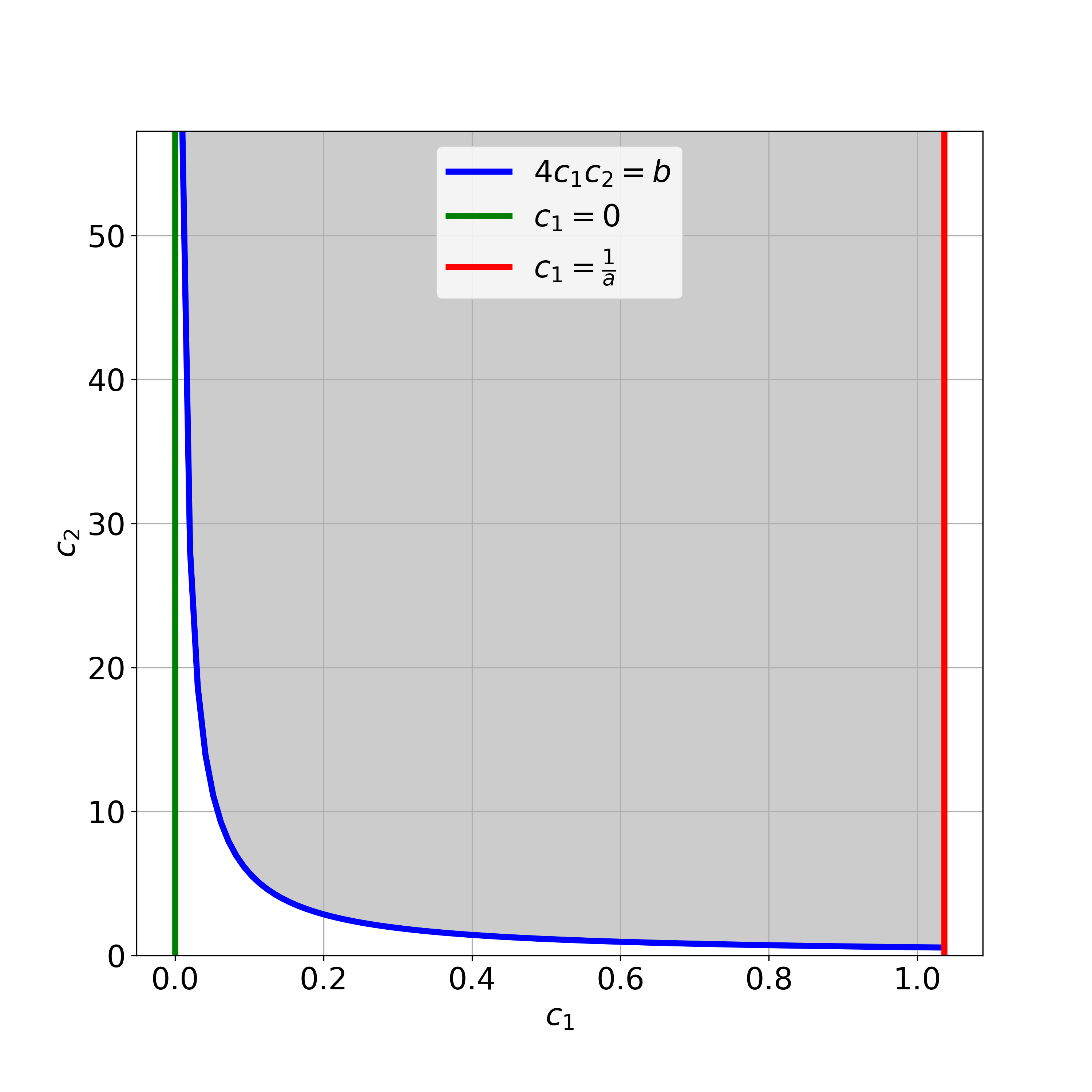
Figure 1: Visualizing optimization problem in Eq. 17.

Since we have

$$\frac{\partial\mathcal{L}(c_{1},c_{2})}{\partial c_{1}} >0$$ (18)

$$\frac{\partial\mathcal{L}(c_{1},c_{2})}{\partial c_{2}} >0$$ (19)

the optimal efficiency prefers small $c_{1}$ and $c_{2}$, and thus the optimal $(c_{1}^{*},c_{2}^{*})$ must be located on the curve $4c_{1}c_{2}=b$. This allows us to further simplify the optimization problem with inequality constraints to one with equality constraints.

$$c_{1}^{*},c_{2}^{*}=\operatorname*{arg\,min}_{\begin{subarray}{c}\{c_{1},c_{2}\}\\ 4c_{1}c_{2}=b\end{subarray}}\mathcal{L}(c_{1},c_{2})$$ (20)

Eq. 20 can be solved by defining another Lagrangian with multiplier $\mu$ as in Eq. 21, and then setting the derivative with respect to the parameters equal to 0.

$$\mathcal{L}(c_{1},c_{2},\mu)\equiv\mathcal{L}(c_{1},c_{2})-\mu(4c_{1}c_{2}-b)$$ (21)

Therefore, the optimal coefficients $(c_{1}^{*},c_{2}^{*})$ is the solution of the system of equations in Eqs. 22 23 24.

$$0 =\frac{\partial\mathcal{L}(c_{1},c_{2},\mu)}{\partial c_{1}}=\frac{e^{c_{2}}}{\left(\frac{1}{a}-c_{1}\right)^{2}}-4\mu c_{2}$$ (22)

$$0 =\frac{\partial\mathcal{L}(c_{1},c_{2},\mu)}{\partial c_{2}}=\frac{e^{c_{2}}}{\frac{1}{a}-c_{1}}-4\mu c_{1}$$ (23)

$$0 =\frac{\partial\mathcal{L}(c_{1},c_{2},\mu)}{\partial\mu}=b-4c_{1}c_{2}$$ (24)

Finally, we find the optimal coefficients as

$$c_{1}^{*} =\frac{2b}{aJ}$$ (25)

$$c_{2}^{*} =\frac{aJ}{8}$$ (26)

where

$$J=\sqrt{b\left(\frac{16}{a}+b\right)}+b$$ (27)

With the optimal coefficients $(c_{1}^{*},c_{2}^{*})$ in Eq. 25 and Eq. 26, Alg. 2 is found to be identical to the “R12” algorithm (Alg. 1) by recognizing the following relationships,

$$c_{1}^{*} =\frac{M}{L}$$ (28)

$$c_{2}^{*} =M$$ (29)

$$h_{1}(x)\leq y\leq h_{2}(x) \Leftrightarrow\left(c_{1}^{*}x+c_{2}^{*}-y\right)^{2}\leq bx$$ (30)

It can also be confirmed that the efficiency of the algorithm (Eq. 11) is equal to $0.7595$ for the case where $a=0.965$ and $b=2.29$. This value is slightly larger than the value of $0.74$ reported in Kalos’ work [5] but can be accurately verified from sampling experiments.

2.4 Alternative $z(x)$ options

In addition to the choice of a linear function of $z(x)$ as in Eq. 5, $z(x)$ in the following form was also explored.

$$z(x)=c_{1}\sqrt{x}+c_{2}$$ (31)

Following a procedure slightly different from above, we will find the optimal coefficients $(c_{1}^{*},c_{2}^{*})$ as

$$c_{1}^{*} =\frac{\sqrt{b}}{2}(1-J_{2})$$ (32)

$$c_{2}^{*} =\frac{(1+J_{2})^{2}}{J_{1}}$$ (33)

where

$$J_{1} =\frac{16}{ab}$$ (34)

$$J_{2} =\sqrt{1+J_{1}}$$ (35)

However, the optimal efficiency which can be described in Eq. 36, is $0.5588$ for the case where $a=0.965$ and $b=2.29$.

$$\eta=\frac{1}{A}\frac{{c_{1}^{*}}^{2}}{e^{c_{2}^{*}}}$$ (36)

Eq. 36 was also numerically verified with Monte Carlo simulation experiments.

3 Conclusions

In this summary, we have re-derived the “R12" algorithm for the Watt spectrum, with a focus on optimizing the efficiency of the rejection sampling method. This bridges the gap in the algorithm, and its interpretation serves as a motivation for enhancing the Watt spectrum sampling technique.

4 Acknowledgments

This work is supported by the Department of Nuclear Engineering, The Pennsylvania State University.

References

- [1] F. B. BROWN, “Monte Carlo Techniques for Nuclear Systems-Theory Lectures,” Tech. rep., Los Alamos National Lab.(LANL), Los Alamos, NM (United States) (2016).
- [2] P. K. ROMANO and B. FORGET, “The OpenMC monte carlo particle transport code,” Annals of Nuclear Energy, 51, 274–281 (2013).
- [3] F. B. BROWN, R. BARRETT, T. BOOTH, J. BULL, L. COX, R. FORSTER, T. GOORLEY, R. MOSTELLER, S. POST, R. PRAEL, ET AL., “MCNP version 5,” Trans. Am. Nucl. Soc, 87, 273, 02–3935 (2002).
- [4] C. J. EVERETT and E. CASHWELL, “MONTE CARLO SAMPLER.” Tech. rep., Los Alamos Scientific Lab., N. Mex. (1972).
- [5] H. GREENSPAN, C. KELBER, and D. OKRENT, Computing methods in reactor physics, Gordon and Breach, New York (1972).
- [6] C. P. ROBERT, G. CASELLA, and G. CASELLA, Monte Carlo statistical methods, vol. 2, Springer (1999).