Deep-Learning-Based Channel Estimation
for IRS-Assisted ISAC System

Abstract

Integrated sensing and communication (ISAC) and intelligent reflecting surface (IRS) are viewed as promising technologies for future generations of wireless networks. This paper investigates the channel estimation problem in an IRS-assisted ISAC system. A deep-learning framework is proposed to estimate the sensing and communication (S&C) channels in such a system. Considering different propagation environments of the S&C channels, two deep neural network (DNN) architectures are designed to realize this framework. The first DNN is devised at the ISAC base station for estimating the sensing channel, while the second DNN architecture is assigned to each downlink user equipment to estimate its communication channel. Moreover, the input-output pairs to train the DNNs are carefully designed. Simulation results show the superiority of the proposed estimation approach compared to the benchmark scheme under various signal-to-noise ratio conditions and system parameters.

I Introduction

The integrated sensing and communication (ISAC) technology has been envisioned as a promising candidate to enhance spectral and energy efficiencies in future generations of wireless networks [1, 2]. To efficiently merge sensing and communication (S&C) functionalities into a single system, the performance trade-off between S&C has recently attracted research attention [3, 4, 5, 6]. The authors in [3] and [4] optimized the sensing functionality, such as the target detection probability and target distance/angle estimation accuracy, while ensured an acceptable communication performance. On the other hand, sensing-assisted communication, which sheds light on how sensing can be co-designed to improve the communication performance including sensing-assisted beam training, tracking, and prediction, is also investigated in [5] and [6]. The above literature generally assumed that the channel state information (CSI) is known at the receiver side and rarely considered the channel estimation problem for the ISAC systems.

Intelligent reflecting surface (IRS) has been foreseen as another promising technology for future wireless networks; it enables the smart and reconfigurable wireless propagation environment [7, 8, 9, 10, 11]. IRS is a programmable planar surface composed of low-cost electromagnetic passive elements. Particularly, based on the CSI of the surrounding wireless environment, IRS can bring outstanding beamforming gain to a communication system by coordinating the reflections of its passive elements. As such, estimating the channels is essential in an IRS-assisted wireless communication system and has been widely researched in the existing literature; it can be classified into conventional model-driven [12] [13] and data-driven deep-learning (DL) approaches [14, 15, 16].

To further enhance the S&C performance, ISAC and IRS have been jointly explored recently [17, 18, 19]. Considering their cooperation merits, the authors in [17] developed an IRS-assisted ISAC framework, which aims to optimize the sensing performance by jointly devising the active and passive beamforming under the constraints of the communication metrics. Moreover, the joint schemes of waveform and passive beamforming design are studied for the IRS-assisted ISAC system in [18] and [19], considering the trade-off between S&C performance. Note that the enhancement of S&C performance builds on the accurate CSI in the above designs. However, to the best of the authors’ knowledge, the channel estimation problem in such IRS-assisted ISAC systems has not been investigated yet in the state-of-art literature.

This paper proposes a DL-based channel estimation approach for the IRS-assisted ISAC system. The key contribution of this work is three-fold:

1. A DL estimation framework, which involves two different deep neural network (DNN) architectures, is developed to estimate the S&C channels. One DNN is employed at the ISAC base station (BS) to estimate the sensing channel between the ISAC BS and the target, while the other one is assigned to each downlink user equipment (UE) for the BS-IRS-UE channel estimation.

2. The generation of the input-output pairs for the DNNs is designed. Moreover, the training data is enriched through augmentation to enhance the estimation performance for both S&C channels.

3. Numerical results demonstrate the substantial improvements achieved by the proposed approach over the benchmark scheme under various signal-to-noise ratio (SNR) conditions and system parameters.

The rest of the paper is organized as follows: In Section II, the S&C models of the IRS-assisted ISAC system are summarized. Section III introduces the proposed DL-based estimation approach. The simulation results and conclusions are provided in Sections IV and V, respectively.

II System Model

Consider an IRS-assisted ISAC system with an ISAC BS, IRS, a target, and $K$ downlink UEs, as illustrated in Fig. 1, where $U_{k}$, $k\in{\mathcal{N}}_{1}^{K}$, denotes the $k$-th UE. Henceforth, ${\mathcal{N}}_{a}^{b}=\{a,a+1,...b\}$ represents the index set from integer $a$ to $b$, and $a<b$. The ISAC BS is equipped with $M$ transmit and $M$ receive antennas to sense the target by utilizing the echo signal from the BS-target-BS channel, ${\mathbf{A}}\in{\mathbb{C}}^{M\times M}$. With the assistance of IRS consisting of $L$ passive reflecting elements, the ISAC BS communicates with the single-antenna downlink UEs through the direct and reflected channels. Let ${\mathbf{b}}_{k}\in{\mathbb{C}}^{M\times 1}$, ${\mathbf{G}}\in{\mathbb{C}}^{M\times L}$, and ${\mathbf{f}}_{k}\in{\mathbb{C}}^{L\times 1}$ denote the channel coefficients of the BS-$U_{k}$, BS-IRS, and IRS-$U_{k}$ links, respectively. Since the ISAC BS transmits and receives signals simultaneously (i.e., full-duplex mode), the self-interference (SI) is induced to the ISAC BS from the SI channel, ${\mathbf{S}}\in{\mathbb{C}}^{M\times M}$.

Fig. 2 shows the pilot transmission protocol that is designed to estimate the channels of the IRS-assisted ISAC system. As seen from Fig. 2, the ISAC BS simultaneously transmits the pilot sequences to the target and UEs in $C$, $C\geq L$, sub-frames, and each sub-frame contains $P$, $P\geq M$, time slots. The pilot signal matrix adopted in the $c$-th, $c\in{\mathcal{N}}_{1}^{C}$, sub-frame is defined as ${\mathbf{X}}=[{\mathbf{x}}_{1},{\mathbf{x}}_{2},\ldots,{\mathbf{x}}_{P}]\in{\mathbb{C}}^{M\times P}$, where ${\mathbf{x}}_{p}\in{\mathbb{C}}^{M\times 1}$ is the pilot signal vector at the $p$-th time slot, $p\in{\mathcal{N}}_{1}^{P}$. Considering the demand for low pilot overhead, let $P=M$ and design ${\mathbf{X}}$ as an $M\times M$ discrete Fourier transform (DFT) matrix, where the $(n,q)$-th entry in ${\mathbf{X}}$ is expressed as ${\bf X}^{(n,q)}=\frac{1}{\sqrt{M}}e^{\jmath\frac{2\pi}{M}nq}$. Furthermore, the IRS phase-shift vector in the $c$-th sub-frame is denoted by ${\mathbf{v}}_{c}\in{\mathbb{C}}^{L\times 1}$. Referring to [14], the phase-shift matrix ${\mathbf{V}}=[{\mathbf{v}}_{1},{\mathbf{v}}_{2},\ldots,{\mathbf{v}}_{C}]\in{\mathbb{C}}^{L\times C}$ is a DFT matrix with $C=L$. This has been proved to be an optimal choice of ${\mathbf{V}}$ to enhance the received signal power at UEs and ensure channel estimation accuracy [14]. Accordingly, it is noted that the ISAC BS sends the identical pilot sequences (i.e., ${\mathbf{X}}$), in each sub-frame. Thus, the IRS phase-shift vector (i.e., ${\mathbf{v}}_{c}$) is kept constant within one sub-frame, whereas it varies among the rest of the sub-frames.

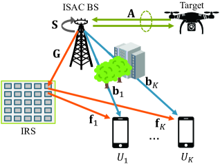
Figure 1: IRS-assisted ISAC system model.                                             

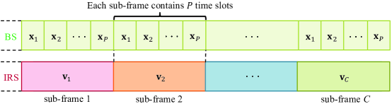
Figure 2: Pilot transmission protocol.                                                      

II-A Sensing Model

Based on the pilot transmission protocol in Fig. 2, the received sensing signal at the $p$-th time slot in the $c$-th sub-frame, ${\mathbf{y}}_{c,p}$, at the ISAC BS is given by

$${\mathbf{y}}_{c,p}=\underbrace{{\mathbf{A}}^{\mathrm{H}}{\mathbf{x}}_{p}}_{\text{Sensing signal}}+\underbrace{{\mathbf{S}}^{\mathrm{H}}{\mathbf{x}}_{p}}_{\text{Residual SI}}+{\mathbf{n}}_{c,p},$$ (1)

where ${\mathbf{n}}_{c,p}\sim{\cal CN}(0,\sigma^{2}{\mathbf{I}}_{M})$ denotes the noise at the ISAC BS that follows the zero-mean complex Gaussian distribution of variance $\sigma^{2}$, with ${\mathbf{I}}_{M}$ as an identity matrix of size $M$. Refer to the radar channel model in [2, 19], the sensing channel is modeled as

$${\mathbf{A}}=\alpha_{\mathrm{S}}{\mathbf{a}}(\theta_{\mathrm{S}}){\mathbf{a}}(\theta_{\mathrm{S}})^{\mathrm{T}},$$ (2)

where $\alpha_{\mathrm{S}}$ represents the complex-valued reflection coefficient of the target. Here, ${\mathbf{a}}(\theta_{\mathrm{S}})$ is the steering vector of the BS transmit antenna array associated with the target’s azimuth angle $\theta_{\mathrm{S}}$ that can be expressed as

$${\mathbf{a}}(\theta_{\mathrm{S}})=[1,e^{\jmath\frac{2\pi{d_{\mathrm{B}}}}{\lambda}\sin(\theta_{\mathrm{S}})},\ldots,e^{\jmath\frac{2\pi{d_{\mathrm{B}}}}{\lambda}({M}-1)\sin(\theta_{\mathrm{S}})}]^{\mathrm{T}},$$ (3)

where $d_{\mathrm{B}}$ and $\lambda$ are the antenna spacing of ISAC BS and the signal wavelength, respectively. Without loss of generality, assume that $d_{\mathrm{B}}=\frac{\lambda}{2}$. The propagation environment between the transmit and received antennas of the ISAC BS is assumed to be slow-changing [20]. Hence, the SI channel, ${\mathbf{S}}$, can be pre-estimated at the ISAC BS, and the residual SI in (1) is compensated before estimating ${\mathbf{A}}$.

II-B Communication Model

For the downlink $U_{k}$, the received signal at the $p$-th time slot in the $c$-th sub-frame, $z_{k,c,p}$, can be expressed as

$$z_{k,c,p}=\underbrace{\Big{(}{\mathbf{b}}_{k}^{\mathrm{H}}+{\mathbf{f}}_{k}^{\mathrm{H}}{\mathrm{diag}}\{{\mathbf{v}}_{c}^{\mathrm{H}}\}{\mathbf{G}}^{\mathrm{H}}\Big{)}{\mathbf{x}}_{p}}_{\text{Downlink communication signal}}+w_{k,c,p},$$ (4)

where ${\mathbf{v}}_{c}=[\beta_{c}e^{\jmath\varphi_{c,1}},\beta_{c}e^{\jmath\varphi_{c,2}},\ldots,$ $\beta_{c}e^{\jmath\varphi_{c,L}}]^{\mathrm{T}}$ with $\beta_{c}\in[0,1]$, and $\varphi_{c,\ell}\in[0,2\pi)$ with $\ell\in{\mathcal{N}}_{1}^{L}$ are the amplitude and phase-shift of the $\ell$-th IRS element, respectively. The noise $w_{k,c,p}$ follows $\mathcal{CN}(0,\varsigma^{2})$ with zero-mean and variance $\varsigma^{2}$. From (4), it is obvious that ${\mathbf{G}}{\mathrm{diag}}\{{\mathbf{v}}_{c}\}{\mathbf{f}}_{k}={\mathbf{G}}{\mathrm{diag}}\{{\mathbf{f}}_{k}\}{\mathbf{v}}_{c}$, where ${\mathrm{diag}}\{\cdot\}$ converts a vector into a diagonal matrix with diagonal elements that are the same as the original vector elements. Thus, the equivalent reflected channel of the BS-IRS-$U_{k}$ link can be expressed as ${\mathbf{B}}_{k}={\mathbf{G}}{\mathrm{diag}}\{{\mathbf{f}}_{k}\}\in{\mathbb{C}}^{M\times L}$. The direct BS-$U_{k}$ channel, ${\mathbf{b}}_{k}$, tends to be blocked by obstacles (e.g., buildings or trees), and the reflected channel is considered [10]. As such, (4) can be rewritten as

$$z_{k,c,p}=\underbrace{{\mathbf{v}}_{c}^{\mathrm{H}}{\mathbf{B}}_{k}^{\mathrm{H}}{\mathbf{x}}_{p}}_{\text{Downlink communication signal}}+w_{k,c,p}.$$ (5)

To model ${\mathbf{B}}_{k}$, the channels of BS-IRS and IRS-$U_{k}$ links, ${\mathbf{G}}$ and ${\mathbf{f}}_{k}$, are modeled as Rician fading [14, 10]. Therefore, ${\mathbf{G}}$ is given by

$${\mathbf{G}}=\sqrt{\frac{K_{\mathrm{BI}}}{K_{\mathrm{BI}}+1}}{\mathbf{G}}_{{\mathrm{LoS}}}+\sqrt{\frac{1}{K_{\mathrm{BI}}+1}}{\mathbf{G}}_{{\mathrm{NLoS}}},$$ (6)

where $K_{\mathrm{BI}}$ represents the Rician factor. Here, ${\mathbf{G}}_{{\mathrm{LoS}}}$ and ${\mathbf{G}}_{{\mathrm{NLoS}}}$ are the line-of-sight (LoS) component and non-LoS (NLoS) component, respectively. In addition, define ${\mathbf{G}}_{{\mathrm{LoS}}}={\mathbf{a}}(\theta_{\mathrm{B}}){\mathbf{a}}(\theta_{\mathrm{I}})^{\mathrm{H}}$, where the steering vectors ${\mathbf{a}}(\theta_{\mathrm{B}})$ and ${\mathbf{a}}(\theta_{\mathrm{I}})$ are formulated similarly as in (3). Particularly, ${\mathbf{a}}(\theta_{\mathrm{B}})$ is associated with the angle of departure (AoD) from the BS to the IRS, $\theta_{\mathrm{B}}$, and the parameters of the BS antenna array (i.e., $M$ and $d_{\mathrm{B}}$), while ${\mathbf{a}}(\theta_{\mathrm{I}})$ is related to the angle of arrival (AoA) at the IRS, $\theta_{\mathrm{I}}$, as well as the parameters of the IRS (i.e., $L$ and inter-element spacing $d_{\mathrm{I}}=\frac{\lambda}{2}$). The IRS-$U_{k}$ channel, ${\mathbf{f}}_{k}$, can be modeled similarly as in (6).

In the following, we aim to estimate the S&C channels, $\{{\mathbf{A}},{\mathbf{B}}_{k}\}$, $k\in{\mathcal{N}}_{1}^{K}$, for the IRS-assisted ISAC system based on the designed pilot transmission protocol.

III Proposed DL-based Estimation Approach

This section proposes a practical channel estimation approach based on DL. The generation of the input-output pairs for the DL networks is firstly designed. On this basis, a DNN-based estimation framework is then developed.

III-A Input-Output Pairs Design

III-A1 Design for Sensing Channel

To generate the input-output pairs of the DL for the sensing channel estimation, $P$ received signal vectors in the $c$-th sub-frame at the ISAC BS (i.e., ${\mathbf{y}}_{c,p}$, $p\in{\mathcal{N}}_{1}^{P}$) are firstly stacked. Since the residual SI is assumed to be compensated, the matrix form of (1) is

$${\mathbf{Y}}_{c}={\mathbf{A}}^{\mathrm{H}}{\mathbf{X}}+{\mathbf{N}}_{c},\quad c\in{\mathcal{N}}_{1}^{C},$$ (7)

where ${\mathbf{Y}}_{c}=[{\mathbf{y}}_{c,1},{\mathbf{y}}_{c,2},\ldots,{\mathbf{y}}_{c,P}]\in{\mathbb{C}}^{M\times P}$ and ${\mathbf{N}}_{c}=[{\mathbf{n}}_{c,1},{\mathbf{n}}_{c,2},\ldots,{\mathbf{n}}_{c,P}]\in{\mathbb{C}}^{M\times P}$. Therefore, the input of the DL, ${\mathbf{R}}^{\mathrm{S}}$, is generated by utilizing the received sensing signals in (7) as

$${\mathbf{R}}^{\mathrm{S}}=\Big{[}\Re\{{\rm{vec}}[{\mathbf{Y}}_{1},{\mathbf{Y}}_{2},\ldots,{\mathbf{Y}}_{C}]\},\Im\{{\rm{vec}}[{\mathbf{Y}}_{1},{\mathbf{Y}}_{2},\ldots,{\mathbf{Y}}_{C}]\}\Big{]}^{\mathrm{T}},$$ (8)

where $\Re\{\cdot\}$ and $\Im\{\cdot\}$ represent the operations of extracting the real and imaginary parts of a complex vector, respectively. $\rm{vec}[\cdot]$ denotes the operation of converting a matrix to a vector. Correspondingly, the output of the DL, ${\mathbf{H}}^{\mathrm{S}}$, is constructed by the ground truth of the sensing channel ${\mathbf{A}}$ as

$${\mathbf{H}}^{{\mathrm{S}}}=\Big{[}\Re\{{\rm{vec}}[{\mathbf{A}}]\},\Im\{{\rm{vec}}[{\mathbf{A}}]\}\Big{]}^{\mathrm{T}}.$$ (9)

Based on the model in (7), the least-squares (LS) estimator is introduced as a benchmark. Define the LS estimation result of the sensing channel as $\bar{}{\mathbf{A}}^{\rm LS}$, which is obtained by

$$\bar{}{\mathbf{A}}^{\rm LS}=\mathbb{E}\big{\{}({\mathbf{Y}}_{c}{\mathbf{X}}^{\dagger})^{\mathrm{H}}\big{\}}={\mathbf{A}}+\mathbb{E}\big{\{}\bar{}{\mathbf{N}}_{c}^{\mathrm{H}}\big{\}},$$ (10)

where ${\mathbf{X}}^{\dagger}={\mathbf{X}}^{\mathrm{H}}({\mathbf{X}}{\mathbf{X}}^{\mathrm{H}})^{-1}$ denotes the pseudoinverse of ${\mathbf{X}}$, $\bar{}{\mathbf{N}}_{c}={\mathbf{N}}_{c}{\mathbf{X}}^{\dagger}$, and $\mathbb{E}\{\cdot\}$ is the expectation operation.

III-A2 Design for Communication Channel

To generate the input-output pairs of the DL for the communication channel estimation, the vector form of (5) is firstly given by

$${\mathbf{z}}_{k,c}={\mathbf{v}}_{c}^{\mathrm{H}}{\mathbf{B}}_{k}^{\mathrm{H}}{\mathbf{X}}+{\mathbf{w}}_{k,c},\quad k\in{\mathcal{N}}_{1}^{K},\quad c\in{\mathcal{N}}_{1}^{C},$$ (11)

where ${\mathbf{z}}_{k,c}=[z_{k,c,1},z_{k,c,2},\ldots,z_{k,c,P}]\in{\mathbb{C}}^{1\times P}$ and ${\mathbf{w}}_{k,c}=[w_{k,c,1},w_{k,c,2},\ldots,w_{k,c,P}]\in{\mathbb{C}}^{1\times P}$. Then, by utilizing the received communication signal in (11), the input of the DL at the downlink $U_{k}$, ${\mathbf{R}}^{U_{k}}$, is generated as

$${\mathbf{R}}^{U_{k}}=\Big{[}\Re\Big{\{}\big{[}{\mathbf{z}}_{k,1},{\mathbf{z}}_{k,2},\ldots{\mathbf{z}}_{k,C}\big{]}\Big{\}},\Im\Big{\{}\big{[}{\mathbf{z}}_{k,1},{\mathbf{z}}_{k,2},\ldots{\mathbf{z}}_{k,C}\big{]}\Big{\}}\Big{]}^{{\mathrm{T}}}.$$ (12)

The corresponding output of the DL at the downlink $U_{k}$, ${\mathbf{H}}^{U_{k}}$, is generated by the ground truth of the communication channel ${\mathbf{B}}_{k}$ as

$${\mathbf{H}}^{U_{k}}=\Big{[}\Re\{{\rm{vec}}[{\mathbf{B}}_{k}]\},\Im\{{\rm{vec}}[{\mathbf{B}}_{k}]\}\Big{]}^{\mathrm{T}}.$$ (13)

According to the model in (11), the LS estimator is adopted as a benchmark at the downlink $U_{k}$, $k\in{\mathcal{N}}_{1}^{K}$. By separating the orthogonal pilot matrix ${\mathbf{X}}$ from ${\mathbf{z}}_{k,c}$ in (11), the derived $\tilde{}{\mathbf{z}}_{k,c}$ is formulated as

$$\tilde{}{\mathbf{z}}_{k,c} ={\mathbf{z}}_{k,c}{\mathbf{X}}^{\dagger}$$

$$={\mathbf{v}}_{c}^{\mathrm{H}}{\mathbf{B}}_{k}^{\mathrm{H}}+\tilde{}{\mathbf{w}}_{k,c},\quad k\in{\mathcal{N}}_{1}^{K},\quad c\in{\mathcal{N}}_{1}^{C},$$ (14)

where $\tilde{}{\mathbf{w}}_{k,c}={\mathbf{w}}_{k,c}{\mathbf{X}}^{\dagger}$. Then, from the first to the $C$-th sub-frames, the matrix form of (14) is written as

$$\tilde{}{\mathbf{Z}}_{k}={\mathbf{V}}^{\mathrm{H}}{\mathbf{B}}_{k}^{\mathrm{H}}+\tilde{}{\mathbf{W}}_{k},\quad k\in{\mathcal{N}}_{1}^{K},$$ (15)

where $\tilde{}{\mathbf{Z}}_{k}=[\tilde{}{\mathbf{z}}_{k,1}^{\mathrm{T}},\tilde{}{\mathbf{z}}_{k,2}^{\mathrm{T}},\ldots,\tilde{}{\mathbf{z}}_{k,C}^{\mathrm{T}}]^{\mathrm{T}}\in{\mathbb{C}}^{C\times M}$ and $\tilde{}{\mathbf{W}}_{k}=[\tilde{}{\mathbf{w}}_{k,1}^{\mathrm{T}},\tilde{}{\mathbf{w}}_{k,2}^{\mathrm{T}},\ldots,\tilde{}{\mathbf{w}}_{k,C}^{\mathrm{T}}]^{\mathrm{T}}\in{\mathbb{C}}^{C\times M}$. Hence, the LS estimate of the BS-IRS-$U_{k}$ channel is

$$\bar{}{\mathbf{B}}_{k}^{\rm LS}=\tilde{}{\mathbf{Z}}_{k}^{\mathrm{H}}{\mathbf{V}}^{\dagger},\quad k\in{\mathcal{N}}_{1}^{K}.$$ (16)

III-A3 Training Dataset Generation

The training dataset of the DL is constructed by the designed input-output pairs. For the sensing channel estimation, define the training dataset as

$$({\mathcal{R}}^{\mathrm{S}},{\mathcal{H}}^{\mathrm{S}})=\Big{\{}\big{(}{\mathbf{R}}^{\mathrm{S}}_{(1,1)},{\mathbf{H}}^{\mathrm{S}}_{(1)}\big{)},\big{(}{\mathbf{R}}^{\mathrm{S}}_{(1,2)},{\mathbf{H}}^{\mathrm{S}}_{(1)}\big{)},\ldots,$$

$$\big{(}{\mathbf{R}}^{\mathrm{S}}_{(1,U)},{\mathbf{H}}^{\mathrm{S}}_{(1)}\big{)},\big{(}{\mathbf{R}}^{\mathrm{S}}_{(2,1)},{\mathbf{H}}^{\mathrm{S}}_{(2)}\big{)},\ldots,\big{(}{\mathbf{R}}^{\mathrm{S}}_{(V,U)},{\mathbf{H}}^{\mathrm{S}}_{(V)}\big{)}\Big{\}},$$ (17)

where $\big{(}{\mathbf{R}}^{\mathrm{S}}_{(v,u)},{\mathbf{H}}^{\mathrm{S}}_{(v)}\big{)}$ denotes the $(v,u)$-th, $v\in{\mathcal{N}}_{1}^{V}$, $u\in{\mathcal{N}}_{1}^{U}$, training sample. Based on the data augmentation, the training samples in this dataset are generated by adopting $V$ received original signals (i.e., sensing signal in (7)), and $U-1$ copies of the $v$-th, $v\in{\mathcal{N}}_{1}^{V}$, are generated by introducing synthetic additive white Gaussian noise to the original channel ${\mathbf{A}}$ with $\text{SNR}_{\text{ch}}=\frac{{\cal P}_{\text{ch}}}{\sigma_{\text{ch}}^{2}}$. Here, ${\cal P}_{\text{ch}}$ and $\sigma_{\text{ch}}^{2}$ represent the power of the original channel ${\mathbf{A}}$ and the synthetic noise, respectively [15]. As such, these noise corrupted channels can be adopted to obtain the copy signals and then generate $U-1$ copy samples, (i.e., $\big{(}{\mathbf{R}}^{\mathrm{S}}_{(v,u)},{\mathbf{H}}^{\mathrm{S}}_{(v)}\big{)}$, $v\in{\mathcal{N}}_{1}^{V}$, $u\in{\mathcal{N}}_{2}^{U}$). In addition to their original versions (i.e., $\big{(}{\mathbf{R}}^{\mathrm{S}}_{(v,1)},{\mathbf{H}}^{\mathrm{S}}_{(v)}\big{)}$, $v\in{\mathcal{N}}_{1}^{V}$), the dataset in (17) is constructed. It is worth mentioning that these copy samples are generated to enrich the training dataset to enhance the estimation performance of the DL network. Moreover, the training dataset for the communication channel estimation, $({\mathcal{R}}^{U_{k}},{\mathcal{H}}^{U_{k}})$, $k\in{\mathcal{N}}_{1}^{K}$, is generated similarly as in (17) at the downlink UE.

III-B Proposed DL Estimation Framework

Based on the designed input-output pairs, the DNN-based estimation framework that consists of the offline training and online testing phases is developed in Fig. 3.

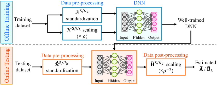
(a)

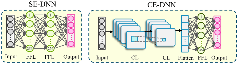
(b)

Figure 3: The proposed DL estimation framework: (a) Offline training and online testing phases, (b) Architectures of the SE-DNN and CE-DNN.

III-B1 Offline Training

For both S&C channel estimation, the offline training phase is composed of the data pre-processing and the network training procedures, as depicted in Fig. 3(a). The data pre-processing is firstly performed on the training dataset, including the input standardization and the output scaling with a factor of $\rho=10^{4}$. Then, the networks in the developed framework are trained by the pre-processed samples to obtain the well-trained networks. Two different DNN architectures are designed to form this framework. The first DNN is devised for the sensing channel estimation, namely sensing estimation DNN (SE-DNN), while the other one is employed for the communication channel estimation, referred to as the communication estimation DNN (CE-DNN).

Here, the detailed offline training procedure for the sensing channel estimation is explained. Given the dataset $({\mathcal{R}}^{\mathrm{S}},{\mathcal{H}}^{\mathrm{S}})$ in (17), the $(v,u)$-th pre-processed input-output pairs in this dataset is obtained as $\big{(}\bar{{\mathbf{R}}}^{\mathrm{S}}_{(v,u)},\bar{{\mathbf{H}}}^{\mathrm{S}}_{(v)}\big{)}$. Then, in the DNN training phase, the designed SE-DNN approximates $\bar{{\mathbf{H}}}^{\mathrm{S}}_{(v)}$ as

$$\bar{{\mathbf{H}}}^{\mathrm{S}}_{(v)}\approx f^{\mathrm{S}}\Big{(}\bar{{\mathbf{R}}}^{\mathrm{S}}_{(v,u)};\Theta^{\mathrm{S}}\Big{)},\quad v\in{\mathcal{N}}_{1}^{V},\quad u\in{\mathcal{N}}_{1}^{U},$$ (18)

where $f^{\mathrm{S}}(\cdot;\Theta^{\mathrm{S}})$ denotes the SE-DNN function and $\Theta^{\mathrm{S}}$ represents all its hyperparameters. The SE-DNN updates $\Theta^{\mathrm{S}}$ by minimizing the mean square error (MSE) of the loss function, ${\cal F}^{\mathrm{S}}$, as

$${\cal F}^{\mathrm{S}}=\frac{1}{VU}\sum_{v\in{\mathcal{N}}_{1}^{V},u\in{\mathcal{N}}_{1}^{U}}\bigg{(}f^{\mathrm{S}}\Big{(}\bar{{\mathbf{R}}}^{\mathrm{S}}_{(v,u)};\Theta^{\mathrm{S}}\Big{)}-\bar{{\mathbf{H}}}_{v}^{\mathrm{S}}\bigg{)}^{2}.$$ (19)

The offline training of the CE-DNN performs similarly to the SE-DNN.

Fig. 3(b) illustrates the architectures of the SE-DNN and CE-DNN. Both consist of the input, hidden, and output layers. Particularly, the hidden layers in the SE-DNN are formed from two feed-forward layers (FFLs) with tanh activation functions. Since the propagation environment of the reflected communication channel is more complicated than that of the sensing channel, the CE-DNN contains three hidden layers that consist of two convolutional layers (CLs) followed by a flatten layer and FFL at the end. The CLs utilize tanh activation functions, while the FFL adopts a linear one. The advantages of this design are attributed to two aspects, as follows. First, the neurons in the CL are connected locally, and partial connections among them share the same weight. Hence, the CL effectively reduces the network parameters and accelerates the convergence compared to the fully connected network [21]. Second, the FFL is further combined with the CL, promoting the channel estimation performance and the generalization capacity of the CE-DNN. For both SE-DNN and CE-DNN, the Adam optimizer is adopted to update the DNN parameters with a learning rate of $2\times 10^{-4}$ and minibatch transitions of size $200$. Moreover, a stopping criterion is applied in the training process, in which the training stops if the validation loss does not improve in $5$ consecutive epochs, or the number of the training epochs reaches $300$. The detailed hyperparameters of the SE-DNN and CE-DNN are summarized in Table I.

TABLE I: Hyperparameters of SE-DNN and CE-DNN

	Layer type	Tensor size	Kernel size	Activation function
SE-DNN	Input	$2MPC$	-	-
	FFL	$256$	-	tanh
	FFL	$256$	-	tanh
	Output	$2M^{2}$	-	-
CE-DNN	Input	$2PC$	-	-
	CL	$128$	$4\times 1$	tanh
	CL	$64$	$4\times 1$	tanh
	FFL	$1024$	-	linear
	Output	$2ML$	-	-

III-B2 Online Testing

Corresponding to the offline training, the online testing phase for the sensing channel estimation is illustrated in Fig. 3(a). The testing dataset, $\dot{{\mathcal{R}}}^{\mathrm{S}}$, is pre-processed to obtain standardized samples that are denoted by $\tilde{{\mathbf{R}}}^{\mathrm{S}}$. Then, the output of the SE-DNN, $\tilde{{\mathbf{H}}}^{\mathrm{S}}$, can be expressed as

$$\tilde{{\mathbf{H}}}^{\mathrm{S}}=f^{\mathrm{S}}(\tilde{{\mathbf{R}}}^{\mathrm{S}};\hat{\Theta}^{\mathrm{S}}),$$ (20)

where $\hat{\Theta}^{\mathrm{S}}$ represents the hyperparameters of the trained SE-DNN. After that, the sensing channel is estimated as $\hat{}{\mathbf{A}}$ by scaling $\tilde{{\mathbf{H}}}^{\mathrm{S}}$ with the factor $\rho^{-1}$ and performing simple matrix operations. Similarly, with the testing dataset, $\dot{{\mathcal{R}}}^{U_{k}}$, at the downlink $U_{k}$, the communication channel is estimated as $\hat{}{\mathbf{B}}_{k}$ by the trained CE-DNN, $f^{U_{k}}(\cdot;\hat{\Theta}^{U_{k}})$. The proposed DNN-based channel estimation algorithm is summarized in Algorithm 1, where $t^{\mathrm{S}}$ and $t^{U_{k}}$ denote the indices of the training epoch used in the S&C channel estimation, respectively.

Algorithm 1 DNN-based Channel Estimation Algorithm.

Initialize: $t^{\mathrm{S}}=0$ and $t^{U_{k}}=0$, $k\in{\mathcal{N}}_{1}^{K}$;
Offline training:

1:  Generate $({\mathcal{R}}^{\mathrm{S}},{\mathcal{H}}^{\mathrm{S}})$ and $({\mathcal{R}}^{U_{k}},{\mathcal{H}}^{U_{k}})$ according to Section III-A;

2:  Pre-process $({\mathcal{R}}^{\mathrm{S}},{\mathcal{H}}^{\mathrm{S}})$ and $({\mathcal{R}}^{U_{k}},{\mathcal{H}}^{U_{k}})$;

3:  Input the pre-processed samples, $\big{(}\bar{{\mathbf{R}}}^{\mathrm{S}}_{(v,u)},\bar{{\mathbf{H}}}^{\mathrm{S}}_{(v)}\big{)}$ and $\big{(}\bar{{\mathbf{R}}}^{U_{k}}_{(v,u)},\bar{{\mathbf{H}}}^{U_{k}}_{(v)}\big{)}$, to the proposed SE-DNN and CE-DNN, respectively;

4:  while the number of epochs does not reach $300$ or the validation accuracy improves in $5$ consecutive epochs do

5:     Update $\Theta^{\mathrm{S}}$ by minimizing ${\cal F}^{\mathrm{S}}$ at the ISAC BS and $\Theta^{U_{k}}$ by minimizing ${\cal F}^{U_{k}}$ at the downlink $U_{k}$, using the Adam optimizer;

6:     Set $t^{\mathrm{S}}\leftarrow t^{\mathrm{S}}+1$ and $t^{U_{k}}\leftarrow t^{U_{k}}+1$;

7:  end while

8:  Output the trained SE-DNN, $f^{\mathrm{S}}(\cdot\,;\hat{\Theta}^{\mathrm{S}})$, at the ISAC BS and the trained CE-DNN, $f^{U_{k}}(\cdot\,;\hat{\Theta}^{U_{k}})$, at the downlink $U_{k}$.

Online testing:

1:  Input: Testing dataset $\dot{{\mathcal{R}}}^{\mathrm{S}}$ and $\dot{{\mathcal{R}}}^{U_{k}}$, $k\in{\mathcal{N}}_{1}^{K}$;

2:     Estimate $\hat{}{\mathbf{A}}$ by using $f^{\mathrm{S}}(\cdot\,;\hat{\Theta}^{\mathrm{S}})$ with the standardized sample $\tilde{{\mathbf{R}}}^{\mathrm{S}}$ at the ISAC BS;

3:     Estimate $\hat{}{\mathbf{B}}_{k}$ by using $f^{U_{k}}(\cdot\,;\hat{\Theta}^{U_{k}})$ with the standardized sample $\tilde{{\mathbf{R}}}^{U_{k}}$ at the downlink $U_{k}$;

4:  Output: Estimated channels $\{\hat{}{\mathbf{A}},\hat{}{\mathbf{B}}_{k}\}$, $k\in{\mathcal{N}}_{1}^{K}$.

IV Simulation Results

This section assesses the performance of the proposed DL-based channel estimation approach for the IRS-assisted ISAC system, considering the LS estimator as benchmark for the comparison. In simulations, $K=3$, $M=4$, and $L=30$ unless further specified. For the sensing channel ${\mathbf{A}}$, the phase-shift of the reflection coefficients are uniformly distributed from $[0,2\pi)$ and $|\alpha_{\mathrm{S}}|=1$ [2]. The azimuth angle of the target is set to $\theta_{\mathrm{S}}=-\frac{2\pi}{3}$. For the communication channels, the AoD and AoA associated with ${\mathbf{G}}_{\mathrm{LoS}}$ are set to $\theta_{\mathrm{B}}=\theta_{\mathrm{I}}=\frac{\pi}{3}$. The Rician factor of the BS-IRS link is $K_{\mathrm{BI}}=10$, while that of the IRS-$U_{k}$ link is $K_{{\mathrm{I}}U_{k}}=0$ [14]. Moreover, the path losses of the S&C channels are $\zeta_{\mathrm{S}}=\zeta_{0}(\frac{d_{\mathrm{S}}}{d_{0}})^{-\gamma_{\mathrm{S}}}$, $\zeta_{\mathrm{BI}}=\zeta_{0}(\frac{d_{\mathrm{BI}}}{d_{0}})^{-\gamma_{\mathrm{BI}}}$, and $\zeta_{{\mathrm{I}}U_{k}}=\zeta_{0}(\frac{d_{{\mathrm{I}}U_{k}}}{d_{0}})^{-\gamma_{{\mathrm{I}}U_{k}}}$, where $\zeta_{0}=-30\,{\rm dBm}$ represents the path loss at the reference distance $d_{0}=1\,\rm m$. The distances of BS-target-BS, BS-IRS, and IRS-$U_{k}$ are set to $d_{\mathrm{S}}=140\,\rm m$, $d_{\mathrm{BI}}=50\,\rm m$, and $d_{{\mathrm{I}}U_{k}}=2\,\rm m$, respectively. The corresponding path loss exponents are $\gamma_{\mathrm{S}}=3$, $\gamma_{\mathrm{BI}}=2.3$, and $\gamma_{{\mathrm{I}}U_{k}}=2$, respectively [10]. The transmit power of the ISAC BS is set to $\mathcal{P}_{0}=20\,\rm dBm$ [22].

The hyperparameters of the proposed SE-DNN and CE-DNN have been summarized in Table I. For both S&C channel estimation, the training dataset size is set to $T_{\rm off}=VU=10^{4}$ for each SNR condition, with $V=10^{3}$, $U=10$, and $\text{SNR}_{\text{ch}}=30\,\rm dB$. Adopt $90\%$ of the dataset for training while the rest for testing. Furthermore, another $T_{\rm on}=10^{3}$ data samples are tested under each SNR condition in the online testing phase. The SNRs at the ISAC BS and the downlink $U_{k}$ are respectively defined as $\text{SNR}_{\mathrm{B}}=\frac{{\cal P}_{\mathrm{B}}}{\sigma^{2}}$ and $\text{SNR}_{U_{k}}=\frac{{\cal P}_{U_{k}}}{\varsigma^{2}}$, where ${\cal P}_{\mathrm{B}}=\mathcal{P}_{0}\zeta_{\mathrm{S}}$ and ${\cal P}_{U_{k}}=\mathcal{P}_{0}\zeta_{\mathrm{BI}}\zeta_{{\mathrm{I}}U_{k}}$ refer to their received signal power. To evaluate the estimation performance, the normalized MSE (NMSE) is employed as performance metric (e.g., NMSE for sensing channel ${\mathbf{A}}$ is denoted by $\text{NMSE}=\mathbb{E}\big{\{}\frac{\|\hat{}{\mathbf{A}}-{\mathbf{A}}\|_{F}^{2}}{\|{\mathbf{A}}\|_{F}^{2}}\big{\}}$, with $\|\cdot\|_{F}$ as the $F$-norm of a matrix).

Fig. 4 studies the effect of the SNR on the S&C channel estimation performance. Let $\text{SNR}=[10,20]\,\rm{dB}$ with a step size of $5\,\rm{dB}$ in the offline training phase, whereas $\text{SNR}=[-10,20]\,\rm{dB}$ with a step size of $2.5\,\rm{dB}$ for online testing. As can be observed, the proposed approach outperforms the benchmark scheme for both ${\mathbf{A}}$ and ${\mathbf{B}}_{k}$. Moreover, it is noted that compared to the benchmark scheme, the proposed approach obtains $15\,\rm dB$ SNR improvement at $\text{NMSE}=10^{-1}$ for the estimation of ${\mathbf{A}}$, while $5\,\rm dB$ SNR improvement at $\text{NMSE}=10^{-1}$ for the estimation of ${\mathbf{B}}_{k}$. The reason is that the sensing channel model in (2) is simpler than the communication one, and thus, the mapping of the input-output pair $({\mathbf{R}}^{\mathrm{S}},{\mathbf{H}}^{\mathrm{S}})$ is more straightforward to be learned by the proposed SE-DNN. Apart from this, Fig. 4 also reveals that the proposed approach possesses considerable generalization ability since the DNNs are trained under several SNR conditions that can be applied to a wide range of SNR regions.

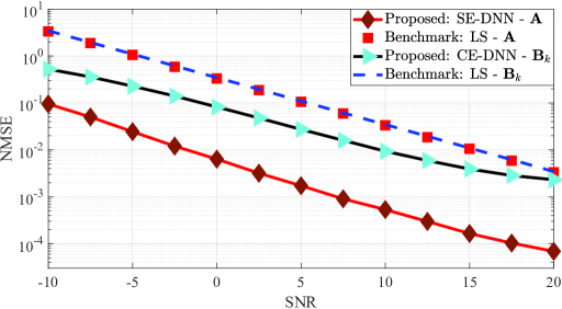
Figure 4: NMSE of S&C channel estimation versus SNR for $M=4$, $L=30$, and $K=3$.

Since $L$ directly affects the dimension of the communication channel ${\mathbf{B}}_{k}$, the impact of varying $L$ on the estimation performance is assessed in Fig. 5. The SNR in the offline training and online testing phases is fixed to $5\,\rm dB$ and $15\,\rm dB$ for CE-DNN. Obviously, the proposed approach provides significant performance improvement compared with the benchmark scheme for different $L$ values and SNR conditions. However, one can note that the NMSE slightly increases as $L$ increases. This may lie in the fact that the mapping of the input-output pair $({\mathbf{R}}^{U_{k}},{\mathbf{H}}^{U_{k}})$ is more difficult to be learned by the CE-DNN when the channel dimension increases, thus, affecting the accuracy of the estimation performance.

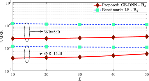
Figure 5: NMSE of communication channel estimation versus $L$ at $M=4$ and $K=3$ for $\text{SNR}=5\,\rm dB$ and $15\,\rm dB$.

Fig. 6 investigates the impact of increasing $M$ on the NMSE performance. The SNR setup is the same as for Fig. 5 with $L=15$. For the estimation performance of ${\mathbf{A}}$ in Fig. 6(a), the NMSE of the proposed approach decreases as $M$ increases and outperforms the benchmark scheme under different SNR conditions. The reason is that the proposed SE-DNN can exploit more distinguishable features of ${\mathbf{A}}$ to enhance the estimation accuracy when the channel dimension becomes larger. Furthermore, the NMSE performance of ${\mathbf{B}}_{k}$ is depicted in Fig. 6(b). Similar to the findings of Fig. 5, the NMSE of ${\mathbf{B}}_{k}$ provided by the proposed approach is superior to that of the benchmark scheme for different $M$ values and SNR conditions, and it slightly increases as $M$ increases.

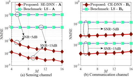
Figure 6: NMSE of S&C channel estimation versus $M$ at $L=15$ and $K=3$ for $\text{SNR}=5\,\rm dB$ and $15\,\rm dB$.

V Conclusion

In this paper, the channel estimation problem for an IRS-assisted ISAC system has been investigated. To estimate the S&C channels effectively, a DL estimation framework realized by the SE-DNN and CE-DNN has been proposed, along with the input-output pairs design. Numerical results have shown that under different SNR conditions, the proposed approach possesses superior generalization ability and significantly improves the NMSE performance compared to the benchmark scheme. Particularly, the SNR improvements of the proposed approach at $\text{NMSE}=10^{-1}$ are up to $15\,\rm dB$ for the sensing channel estimation, while $5\,\rm dB$ for the communication one. Furthermore, the proposed approach has been evaluated under a wide range of channel dimensions and results revealed a considerable NMSE performance improvement over the benchmark scheme.

References

- [1] F. Liu, Y. Cui, C. Masouros, J. Xu, T. X. Han, Y. C. Eldar, and S. Buzzi, “Integrated sensing and communications: Towards dual-functional wireless networks for 6G and beyond,” arXiv preprint arXiv:2108.07165, 2021.
- [2] F. Liu, C. Masouros, A. P. Petropulu, H. Griffiths, and L. Hanzo, “Joint radar and communication design: Applications, state-of-the-art, and the road ahead,” IEEE Trans. Commun., vol. 68, no. 6, pp. 3834–3862, Jun. 2020.
- [3] B. K. Chalise, M. G. Amin, and B. Himed, “Performance tradeoff in a unified passive radar and communications system,” IEEE Signal Process. Lett., vol. 24, no. 9, pp. 1275–1279, Sep. 2017.
- [4] F. Liu, Y. Liu, A. Li, C. Masouros, and Y. C. Eldar, “Cramer-rao bound optimization for joint radar-communication beamforming,” IEEE Trans. Signal Process., vol. 70, pp. 240–253, 2022.
- [5] F. Liu, W. Yuan, C. Masouros, and J. Yuan, “Radar-assisted predictive beamforming for vehicular links: Communication served by sensing,” IEEE Trans. Wireless Commun., vol. 19, no. 11, pp. 7704–7719, Nov. 2020.
- [6] W. Yuan, F. Liu, C. Masouros, J. Yuan, D. W. K. Ng, and N. González-Prelcic, “Bayesian predictive beamforming for vehicular networks: A low-overhead joint radar-communication approach,” IEEE Trans. Wireless Commun., vol. 20, no. 3, pp. 1442–1456, Mar. 2021.
- [7] Q. Wu, S. Zhang, B. Zheng, C. You, and R. Zhang, “Intelligent reflecting surface-aided wireless communications: A tutorial,” IEEE Trans. Commun., vol. 69, no. 5, pp. 3313–3351, May 2021.
- [8] I. Al-Nahhal, O. A. Dobre, E. Basar, T. M. N. Ngatched, and S. Ikki, “Reconfigurable intelligent surface optimization for uplink sparse code multiple access,” IEEE Commun. Lett., vol. 26, no. 1, pp. 133–137, Jan. 2022.
- [9] I. Al-Nahhal, O. A. Dobre, and E. Basar, “Reconfigurable intelligent surface-assisted uplink sparse code multiple access,” IEEE Commun. Lett., vol. 25, no. 6, pp. 2058–2062, Jun. 2021.
- [10] A. Faisal, I. Al-Nahhal, O. A. Dobre, and T. M. N. Ngatched, “Deep reinforcement learning for optimizing RIS-assisted HD-FD wireless systems,” IEEE Commun. Lett., vol. 25, no. 12, pp. 3893–3897, Dec. 2021.
- [11] R. Zhong, X. Liu, Y. Liu, Y. Chen, and Z. Han, “Mobile reconfigurable intelligent surfaces for NOMA networks: Federated learning approaches,” IEEE Trans. Wireless Commun., Early access, 2022.
- [12] X. Wei, D. Shen, and L. Dai, “Channel estimation for RIS assisted wireless communications–Part I: Fundamentals, solutions, and future opportunities,” IEEE Commun. Lett., vol. 25, no. 5, pp. 1398–1402, May 2021.
- [13] Z. He and X. Yuan, “Cascaded channel estimation for large intelligent metasurface assisted massive MIMO,” IEEE Wireless Commun. Lett., vol. 9, no. 2, pp. 210–214, Feb. 2020.
- [14] C. Liu, X. Liu, D. W. K. Ng, and J. Yuan, “Deep residual learning for channel estimation in intelligent reflecting surface-assisted multi-user communications,” IEEE Trans. Wireless Commun., vol. 21, no. 2, pp. 898–912, Feb. 2022.
- [15] A. M. Elbir, A. Papazafeiropoulos, P. Kourtessis, and S. Chatzinotas, “Deep channel learning for large intelligent surfaces aided mm-wave massive MIMO systems,” IEEE Wireless Commun. Lett., vol. 9, no. 9, pp. 1447–1451, May 2020.
- [16] M. Xu, S. Zhang, J. Ma, and O. A. Dobre, “Deep learning-based time-varying channel estimation for RIS assisted communication,” IEEE Commun. Lett., vol. 26, no. 1, pp. 94–98, Jan. 2022.
- [17] Z. Jiang, M. Rihan, P. Zhang, L. Huang, Q. Deng, J. Zhang, and E. M. Mohamed, “Intelligent reflecting surface aided dual-function radar and communication system,” IEEE Syst. J., pp. 1–12, 2021.
- [18] X. Wang, Z. Fei, Z. Zheng, and J. Guo, “Joint waveform design and passive beamforming for RIS-assisted dual-functional radar-communication system,” IEEE Trans. Veh. Technol., vol. 70, no. 5, pp. 5131–5136, May 2021.
- [19] X. Wang, Z. Fei, J. Huang, and H. Yu, “Joint waveform and discrete phase shift design for RIS-assisted integrated sensing and communication system under cramer-rao bound constraint,” IEEE Trans. Veh. Technol., vol. 71, no. 1, pp. 1004–1009, Jan. 2022.
- [20] R. Mai, D. H. N. Nguyen, and T. Le-Ngoc, “Joint MSE-based hybrid precoder and equalizer design for full-duplex massive MIMO systems,” in Proc. IEEE ICC, May 2016, pp. 1–6.
- [21] Z. Li, F. Liu, W. Yang, S. Peng, and J. Zhou, “A survey of convolutional neural networks: Analysis, applications, and prospects,” IEEE Trans. Neural Netw. Learn. Syst., Early Access, 2021.
- [22] T. Jiang, H. V. Cheng, and W. Yu, “Learning to reflect and to beamform for intelligent reflecting surface with implicit channel estimation,” IEEE J. Sel. Areas Commun., vol. 39, no. 7, pp. 1931–1945, Jul. 2021.