What Is a Causal Graph?

Abstract

This article surveys the variety of ways in which a directed acyclic graph (DAG) can be used to represent a problem of probabilistic causality. For each of these we describe the relevant formal or informal semantics governing that representation. It is suggested that the cleanest such representation is that embodied in an augmented DAG, which contains nodes for non-stochastic intervention indicators in addition to the usual nodes for domain variables.

Keywords: directed acyclic graph; extended conditional independence; augmented DAG; moralisation; structural causal model

1 Introduction

Graphical representations of probabilistic (Pearl, 1988, Lauritzen, 1996, Cowell et al., 1999) and causal (Pearl, 2009) problems are ubiquitous. Such a graph has nodes representing relevant variables in the system, which we term domain variables, and arcs between some of the nodes. The most commonly used type of graph for these purposes, to which we will confine attention in this article, is a Directed Acyclic Graph (DAG), in which the arcs are arrows, and it is not possible to return to one’s starting point by following the arrows. An illustration of such a DAG (Dawid and Evett, 1997) is given in Figure 1.

Figure 1: Directed acyclic graph ${\cal D}$

Now there is no necessary relationship between a geometric object, such as a graph, and a probabilistic or causal model—they inhabit totally different mathematical universes. Any such relationship must therefore be specified externally, and then constitutes a way of interpreting the graph as saying something about the problem at hand. It is important to distinguish between the syntax of a graph, i.e., its internal, purely geometric properties, and its semantics, describing its intended interpretation.

In this article we consider a variety of ways—some formal, some less so—in which DAGs have been and can be interpreted. In particular, we emphasise the importance of a clear understanding of what is the intended interpretation in any specific case. We caution against the temptation to interpret purely syntactical elements, such as arrows, semantically (the sin of “reification”), or to slide unthinkingly from one interpretation of the graph to another.

The material in this article is largely a survey of previously published material (Dawid, 2002, 2003, 2010a, 2010b, 2015, 2021, 2022, Dawid and Didelez, 2010, Geneletti and Dawid, 2011, Dawid et al., 2017, Dawid and Musio, 2022, Constantinou and Dawid, 2017, Dawid et al., 2022), which should be consulted for additional detail and discussion. In particular we do not here showcase the wealth of important applications of the methods discussed.

Outline

In § 2 we describe how a DAG can be used to represent properties of probabilistic independence between variables, using a precise semantics based on the method of moralisation. An alternative representation, involving functional rather than probabilistic dependencies, is also presented. Section 3 discusses some informal and imprecise ways in which a DAG might be considered as representing causal relations. In preparation for a more formal approach, § 4 describes an understanding of causality as a reaction to an external intervention in a system, and presents an associated language, based on an extension of the calculus of conditional independence, for expressing and manipulating causal concepts. Turning back to a DAG model, in § 5 we introduce a precise semantics for its causal interpretation, again based on moralisation, this time used to express extended condtional independence properties. To this end we introduce augmented DAGs, which contain nodes for non-stochastic intervention indicators, as well as for stochastic domain variables. In § 6 we describe the causal semantics of a “Pearlian” (Pearl, 2009) DAG, and show how these can be explicitly represented by an augmented DAG, where again a version involving functional relationships—the Structural Causal Model (SCM) —is available.

Section 7 considers a different type of causal problem, that is not about the response of a system to an intervention, but rather aims to assign, to an observed putative cause, responsibility for the emergence of an observed outcome. This requires new understandings and semantics that can not be represented by a probabilistic DAG, but can be by using a structural causal model. However this is problematic, since there can be distinct SCMs that are observationally equivalent but lead to different answers.

2 Probabilistic DAG

The most basic way of interpreting a DAG is as representing qualitative probabilistic relations of conditional independence between its variables. Such a situation occupies the lowest rung of the “ladder of causaton” (Pearl and Mackenzie, 2018). The semantics governing such a representation, while precise, are not totally straightforward, being described by either of two logically equivalent criteria, known as “$d$-separation” (Pearl, 1986, Verma and Pearl, 1990) and “moralisation” (Lauritzen et al., 1990). Here we describe moralisation, using the specific DAG ${\cal D}$ of Figure 1 for illustration.

Suppose we ask: Is the specific conditional independence property

$$(B,R)\,\mbox{$\perp\!\!\!\perp$}\,(G_{1},Y_{1})\mid(A,N)$$

(read as “the pair $(B,R)$ is independent of $(G_{1},Y_{1})$, conditional on $(A,N)$”—see Dawid (1979)) represented by the graph? To address this query we proceed as follows:

1. Ancestral graph

We form a new DAG ${\cal D}^{\prime}$ by removing from ${\cal D}$ every node that is not mentioned in the query and is not an ancestor of a mentioned node, as well as any arrow involving a removed node. Figure 2 shows the result of applying this operation to Figure 1.

Figure 2: Ancestral subgraph ${\cal D}^{\prime}$

2. Moralisation

If in ${\cal D}^{\prime}$ there are two nodes that have a common child (i.e., each has an arrow directed from it to the child node) but they are not themselves joined by an arrow—a configuration termed an “immorality”—then an undirected edge is inserted between them. Then every remaining arrowhead is removed, yielding an undirected graph ${\cal G}^{\prime}$. In our example this yields Figure 3.

Figure 3: Moralised ancestral subgraph ${\cal G}^{\prime}$

3. Separation

Finally, in ${\cal G}^{\prime}$ we look for a continuous path connecting an element of the first set in our query (here $(B,R)$) to an element of the second set (here $(G_{1},Y_{1})$) that does not contain an element of the third set (here $(A,N)$). If there is no such path, we conclude that the queried conditional independence property is represented in the original DAG. Since this is the case in our example, the property $(B,R)\,\mbox{$\perp\!\!\!\perp$}\,(G_{1},Y_{1})\mid(A,N)$ is indeed represented in Figure 1.

2.1 Instrumental variable

The DAG of Figure 4 can be used to represent a problem in which we have an “instrumental variable”, with the nodes interpreted as follows:

$X$

Exposure

$Y$

Outcome

$Z$

Instrument

$U$

Unobserved confounding variables

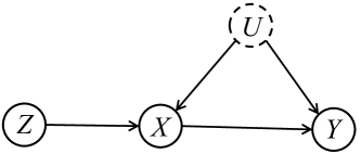
Figure 4: Instrumental variable

Such a problem invites a causal interpretation, which we will take up in § 5 below. But if we interpret Figure 4 purely as a probabilistic DAG, we see that it represents exactly the following conditional independencies:

$$U \perp\!\!\!\perp Z$$ (1)

$$Y \perp\!\!\!\perp Z\mid(U,X)$$ (2)

2.2 Markov equivalence

Given a collection of conditional independence relations for a set of variables, there may be $0$, $1$, or several DAGs that represent just these relations. Two DAGs are termed Markov equivalent when they represent the identical conditional independencies. It can be shown (Frydenberg, 1990, Verma and Pearl, 1991) that this will be the case if they have the same skeleton (i.e., the undirected graph obtained by deleting the arrowheads) and the same immoralities.

Example 1

Consider the following DAGs on three nodes:

1. $A\to B\to C$

2. $A\leftarrow B\leftarrow C$

3. $A\leftarrow B\to C$

4. $A\to B\leftarrow C$.

These all have the same skeleton. However, whereas DAGs 1, 2 and 3 have no immoralities, 4 has one immorality. Consequently, 1, 2 and 3 are all Markov equivalent, but 4 is not Markov equivalent to these. Indeed, 1, 2 and 3 all represent the conditional independence property $A\,\mbox{$\perp\!\!\!\perp$}\,C\mid B$, whereas 4 represents the marginal independence property $A\,\mbox{$\perp\!\!\!\perp$}\,C$. $\Box$

2.3 Bayesian network

The purely qualitative graphical structure of a probabilistic DAG can be elaborated with quantitative information. With each node in the DAG we associate a specified conditional distribution for its variable, given any values for its parent variables. There is a one-one correspondence between a collection of all such parent-child distributions and a joint distribution for all the variables that satisfies all the conditional independencies represented by the graph. The graphical structure also supports elegant algorithms for computing marginal and conditional distributions (Cowell et al., 1999).

2.4 Structural probabilistic model

Suppose we are given the conditional distribution $p(Y\mid X)$. It is then possible to construct (albeit non-uniquely) a fictitious “error variable” $E$, having a suitable distribution $P$, and a suitable deterministic function $f$ of $(X,E)$, such that the distribution of $f(x,E)$ is just $p(Y\mid X=x)$. For example, using the probability integral transform, if $F_{x}$ is the cumulative distribution function of $p(Y\mid X=x)$, we can take $f(x,e)=F_{x}^{-1}(e)$ and $E$ uniform on $[0,1]$. However such a representation is highly non-unique. Indeed, we could alternatively take $f(x,e)=F_{x}^{-1}(e_{x})$, where $e$ is now a vector $(e_{x})$, and the multivariate distribution of $E$ is an arbitrarily dependent copula, such that each entry $(E_{x})$ is uniform on $[0,1]$.

Given any such construction, for purely distributional purposes we can work with the functional equation $Y=f(X,E)$, with $E\sim P$ independently of $X$. This operation can be extended to apply to a complete Bayesian network, by associating with each domain variable $V$ a new error variable $E_{V}$, with suitable distribution $P_{v}$, all these being independent, and with $V$ being modelled as a suitable determistic function of its graph parent domain variables and $E_{V}$. We term such a deterministic model a Structural Probabilistic Model (SPM), by analogy with the Structural Causal Model (SCM) (Pearl and Mackenzie, 2018)—see § 6.1 below. In an SPM, all stochasticity is confined to the error variables.

An SPM can be represented graphically by introducing new nodes for the error variables, as illustrated in Figure 5 for the case of Figure 4, it being understood that the error variables are modelled as random, but all other parent-child relations are deterministic.

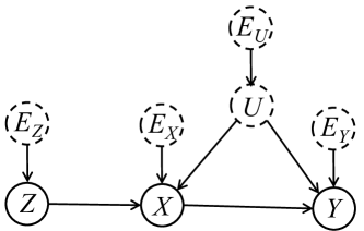
Figure 5: SPM representation of instrumental variable model

It is easy to check that the conditional independencies represented between the domain variables, as revealed by the moralisation criterion, are identical, both in the original graph and in an SPM extension of it. So, when each graph is endowed with its own parent-child relationships (stochastic in the case of the original graph, deterministic for the structural graph), both graphs describe the identical joint distribution for the domain variables. For purely probabilistic purposes, nothing is gained by introducing error variables to “mop up” the stochastic dependencies of a simple DAG model.

2.5 Reification?

It is important to keep in mind that a probabilistic DAG is nothing but a very indirect way of representing a collection of conditional independence properties. In particular, the arrows in the DAG have no intrinsic meaning, being there only to support the moralisation procedure. It is indeed somewhat odd that the property of conditional independence, which is essentially a symmetric one, can be represented at all by means of arrows, which have built-in directionality. The example of Markov equivalence between 1, 2 and 3 in Example 1 shows that the specific direction of an arrow in a DAG should not be taken as meaningful itself. Rather, an arrow has a transient status rather like that of a construction line in an architect’s plan, or of a contour line on a map: instrumentally helpful, but not representing anything visible in the house or on the ground.

Nevertheless, on looking at a DAG, it is hard to avoid the temptation to imbue its arrows with a direct meaning in relation to the system studied. This is the philosophical error of reification, which confuses the map with the territory (Korzybski, 1933), wrongly interpreting a purely instrumental property of a representation as if it had a direct counterpart in the external system. In the case of a probabilistic DAG model, this frequently leads to endowing it with an unjustified causal interpretation, where the presence of an arrow $A\rightarrow B$ is considered to represent the presence of a causal influence of $A$ on $B$. Such a confusion underlies much of the enterprise of “causal discovery”, where observational data are analysed to uncover their underlying probabilistic conditional indepencies, these are represented by a probabilistic DAG, and that DAG is then reinterpreted as representing causal relations.

This is not to say that a DAG can not be interpreted causally—but to do so will require a fresh start, with new semantics.

3 Informal causal semantics

Common causal interpretations of a DAG involve statements such as:

• an arrow represents a direct cause

• a directed path represents a causal pathway

Or, as described for example by Hernán and Robins (2006):

“A causal DAG ${\cal D}$ is a DAG in which:

1. the lack of an arrow from $V_{j}$ to $V_{m}$ can be interpreted as the absence of a direct causal effect of $V_{j}$ on $V_{m}$ (relative to the other variables on the graph)

2. all common causes, even if unmeasured, of any pair of variables on the graph are themselves on the graph.

Thus Figure 4 might be interpreted as saying:

• $U$ is a common cause of $X$ and $Y$

• $Z$ affects the outcome $Y$ only through $X$

• $Z$ does not share common causes with $Y$

• $Z$ has a direct causal effect on $X$

In the above, we have marked syntactical terms, relating to the graph itself (the “map”), in bold-face, and terms involving external concepts (the “territory”), in teletype.

3.1 Probabilistic Causality

Or, one can start by ignoring the DAG, and try to relate causal concepts directly to conditional independence. Such an approach underlies the enterprise of causal discovery, where discovered conditional independencies are taken to signify causal relations. Common assumptions made here are:

Weak Causal Markov assumption:

If $X$ and $Y$ have no common cause (including each other), they are probabilistically independent

Causal Markov assumption:

A variable is probabilistically independent of its non-effects, given its direct causes

Conbining such assumptions with the formal semantics by which a DAG represents conditional independence, we obtain a link between the DAG and causal concepts.

3.2 A problem

How could we check if a DAG, endowed with a causal interpretation along the above lines, is a correct representation of the external problem it is intended to model? To even begin to do so, we would already need to have an independent understanding of the external concepts, as marked in bold-face—which thus can not make reference to the graph itself. But these informal causal concepts are woolly and hard to pin down. I am aware of almost no work that even attempts to do so—a recent exception is Sadeghi and Soo (2023). But without this, using such informal causal semantics risks generating confusion rather than clarification.

To avoid confusion, we need to develop a more formal causal semantics.

4 Interventional causality and extended conditional independence

Our approach to this begins by introducing an explicit, non-graphical, understanding of causality, expressed in terms of the probabilistic response of a system to an (actual or proposed) intervention. A causal effect of $A$ on $B$ exists if the distribution of $B$, after an external intervention sets $A$ to some value $a$, varies with $a$. Formally we introduce a non-stochastic variable $F_{A}$, having the same set of values as $A$, such that $F_{A}=a$ describes the regime in which $A$ is set to value $a$ by an external intervention. Then $A$ has no causal effect on $B$ just when the distribution of $B$, given $F_{A}=a$, does not depend on $a$.

If $F_{A}$ were a stochastic variable, this would just be the usual property of independence of $B$ from $F_{A}$, notated as

$$\mbox{$B\,\mbox{$\perp\!\!\!\perp$}\,F_{A}$}.$$ (3)

Now not only does this understanding of independence remain intuitively meaningful in the current case that $F_{A}$ is a non-stochastic variable, but the formal mathematical properties of independence and conditional independence can be rigorously extended to such cases (Dawid, 1979, 1980, Constantinou and Dawid, 2017): we term this extended conditional independence (ECI). The standard axioms of conditional independence apply, with essentially no changes, to ECI.

Since much of the enterprise of statistical causality involves drawing causal conclusions from observational data, we further endow $F_{A}$ with an additional state $\emptyset$, read as “idle”: $F_{A}=\emptyset$ denotes the regime in which no intervention is applied to $A$, but it is allowed to develop “naturally”, in the observational setting. The distinction between $A$ and $F_{A}$ is that the state of $A$ describes what value was taken, while the state of $F_{A}$ describes how that value was taken.

We regard the main thrust of causal statistical inference as aiming to deduce properties of a hypothetical interventional regime, such as the distribution of $B$ given $F_{A}=a$, from observational data, obtained under the idle regime $F_{A}=\emptyset$. But since there is no logically necessary connexion between the distributions under different regimes, suitable assumptions will need to be made—and justified—to introduce such connexions.

The simplest such assumption—which, however will only very rarely be justifiable—is that when we consider the distribution of $B$ given $A$, we need to know what was the value $a$ that $A$ took, but not how it came to take that value (i.e., not whether this was in the observational regime $F_{A}=\emptyset$, or in the interventional regimes, $F_{A}=a$), the conditional distribution of $B$ being the same in both cases. That is,

$$p(B=b\mid A=a,F_{A}=\emptyset)=p(B=b\mid A=a,F_{A}=a).$$ (4)

This is the property of ignorability. When this strong property holds, we can directly take the observed distribution of $B$ given $A=a$ for the desired interventional distribution of $B$ given $F_{A}=a$: the distribution of $B$ given $A$ is a “modular component”, transferable between different regimes.

We note that (4) can be expressed succinctly using ECI notation, as

$$B\,\mbox{$\perp\!\!\!\perp$}\,F_{A}\mid A$$ (5)

As exemplified by (3) and (5), ECI supplies a simple and powerful language for expressing and manipulating causal concepts.

5 Augmented DAG

We can now introduce a formal graphical causal semantics, so moving onto the second rung of the ladder of causation. This is based on ECI, represented by an augmented DAG, which is just like a regular DAG, except that some of its nodes may represent non-stochastic variables, such as regime indicators. Just as certain collections of purely probabilistic conditional independence properties can usefully and precisely be represented (by moralisation) by means of a regular DAG, so we may be able to construct an augmented DAG to represent (by exactly the same moralisation criterion) causal properties of interest expressed in terms of ECI.

Consider for example the simple augmented DAG

$$F_{A}\rightarrow A\rightarrow B$$

This represents (by moralisation, as always) the ECI property of (5), and so is a graphical representation of the ignorability assumption. Note that it is the whole structure that, with ECI, imparts causal meaning to the arrow from $A$ to $B$—the direction of that arrow would not otherwise be meaningful in itself.

Example 2

Consider the following augmented DAGS, modifications of the first three DAGs of Example 1 to allow for an intervention on $A$:

1. $F_{A}\to A\to B\to C$

2. $F_{A}\to A\leftarrow B\leftarrow C$

3. $F_{A}\to A\leftarrow B\to C$

We saw in Example 1 that, without the node $F_{A}$, these DAGs are all Markov equivalent. With $F_{A}$ included, we see that DAGs 2 and 3 are still Markov equivalent, since they have the same skeleton and the same unique immorality $F_{A}\to A\leftarrow B$; but they are no longer Markov equivalent to DAG 1, which does not contain that immorality. All three DAGs represent the ECI $A\,\mbox{$\perp\!\!\!\perp$}\,C\mid(F_{A},B)$, which says that, in any regime, $A$ is independent of $C$ given $B$; however, while DAGs 2 and 3 both represent the ECI $(B.,C)\,\mbox{$\perp\!\!\!\perp$}\,F_{A}$, which implies that $A$ does not cause either $B$ or $C$, DAG 1 instead represents the ECI $(B,C)\,\mbox{$\perp\!\!\!\perp$}\,F_{A}\mid A$, expressing the ignorability of the distribution of $(B,C)$ given $A$.

Note moreover that the Markov equivalence of DAGs 2 and 3 means that we can not interpret the direction of the arrow between $B$ and $C$ as meaningful in itself. In particular, in DAG 3 the arrow $B\rightarrow C$ does not signify a causal effect of $B$ on $C$: in this approach, causality is only described by ECI properties, and their moralisation-based graphical representations. $\Box$

Example 3

To endow the instrumental variable problem of Figure 4 with causal content—specifically, relating to the causal effect of $X$ on $Y$—we might replace it by the augmented DAG of Figure 6, where the node $F_{X}$ now allows us to consider an intervention on $X$.

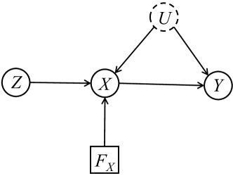
Figure 6: Instrumental variable: Augmented DAG

This DAG still represents the probabilistic conditional independencies (1) and (2), in any regime. But now it additionally represents genuine causal properties:

$$(U,Z) \perp\!\!\!\perp F_{X}$$ (6)

$$Y \perp\!\!\!\perp F_{X}\mid(Z,U,X)$$ (7)

Property (6) says that $X$ has no causal effect on $U$ and $Z$, these having the same joint distribution in all regimes (including the idle regime). Property (7) entails the modular conditional ignorability property that the distribution of $Y$ given $(z,u,x)$ (which in fact depends only on $(u,x)$, by (1)) is the same, both in the interventional regime where $X$ is set to $x$, and in the observational regime where $X$ is not controlled. Although rarely stated so explicitly, these assumptions are basic to most understandings of an instrumental variable problem, and its analysis (which we shall not however pursue here).

If we wanted, we could work with an augmented version of the SPM representation of Figure 5, as in Figure 7.

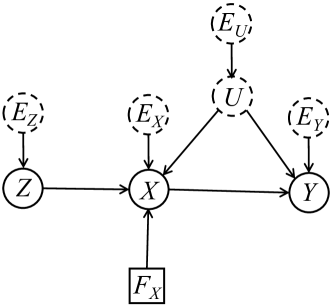
Figure 7: Instrumental variable: Augmented DAG with error variables

This entails exactly the same ECI properties as Figure 6 for the domain variables and the intervention variable. With suitably chosen distributions for the error variables and functional dependence of each domain variable on its parents, we can recover the same joint distribution for the domain variables, in any regime, as in the original probabilistic augmented DAG. Inclusion of the extra structure brings nothing new to the table.

Yet another representation of the problem is given in Figure 8.

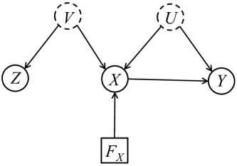
Figure 8: Instrumental variable: Alternative augmented DAG

Here $V$ denotes an additional unobserved variable of no direct interest. It can again be checked that both Figure 6 and Figure 8 represent the identical ECI properties between the variables of interest, $X,Y,Z,U$ and $F_{X}$. This identity shows that the arrow $Z\rightarrow X$ in Figure 6 should not be taken as signifying a direct causal effect of $Z$ on $X$: we could equally well regard $X$ and $Z$ as being associated through a common cause, $V$. Hernán and Robins (2006) regard Figure 6 and Figure 8 as essentially different—as indeed they would be if interpreted in these informal terms—and conclude (correctly) that it is not necessary, for analysing the instrumental variable problem, to require that $Z$ have a direct effect on $X$. From our point of view there is no essential difference between Figure 6 and Figure 8, since even in Figure 6 the arrow $Z\rightarrow X$ should not be interpreted causally. $\Box$

6 Pearlian DAG

C onsider the DAG of Figure 9.

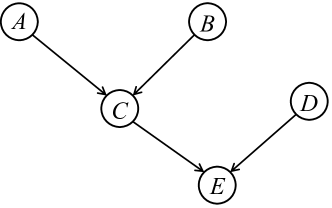
Figure 9: Pearlian DAG

As it stands this looks like a probabilitic DAG, representing purely conditional independence properties, such as $C\,\mbox{$\perp\!\!\!\perp$}\,D\mid(A,B)$. Pearl (2009), however, would endow it with additional causal meaning, using an interventional interpretation as in § 4. He would regard it as asserting that, for any node, its conditional distribution, given its parents, would be the same, in a purely observational setting, and in any interventional setting that sets the values of some or all of the variables other than itself. For example, it requires:

The distribution of $C$, given $(A,B)$, does not depend on whether $A$ and $B$ arose naturally, or were set by external intervention.

While this is a perfectly clear formal interpretation of Figure 9, it is problematic in that, if we are just presented with that DAG, we may not know whether it is meant to be interpreted as representing only probabilistic properties, or is supposed to be further endowed with Pearl’s causal semantics. This ambiguity can lead to confusion: a particular danger is to see, or construct, a probabilistic DAG, and then slide, unthinkingly, into giving it an unwarranted Pearlian causal interpretation.

We can avoid this problem by explicit inclusion of regime indicators, one for each domain variable, as for example in Figure 10.

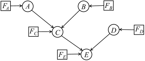
Figure 10: Augmented Pearlian DAG

Not only is this clearly not intended as a probabilistic DAG, but the Pearlian causal semantics, which in the case of Figure 9 require external specification, are now explicitly represented in the augmented DAG, by moralisation. For example, Figure 10 represents the ECI $C\,\mbox{$\perp\!\!\!\perp$}\,(F_{A},F_{B})\mid(A,B,F_{C},F_{D},F_{E})$. When $F_{C}=c\neq\emptyset$, $C$ has a one-point distribution at $c$, and this ECI holds trivially. But for $F_{C}=\emptyset$ we recover the property quoted in italics above (under any settings, idle or interventional, of $F_{D}$ and $F_{E}$).

We also note that an augmented Pearlian DAG can have no other Markov equivalent such DAG, since no arrow can be reversed without creating or destroying an immorality. In this sense every arrow now carries causal meaning.

However, just as we should not automatically interpret a regular DAG as Pearlian, so we should not unthinkingly simply augment it by adding an intervention indicator for each domain variable—which would have the same effect. We must consider carefully whether the many very strong properties embodied in any Pearlian or augmented DAG, relating probabilistic properties (parent-child distributions) across distinct regimes, are justifiable in the specific applied context we are modelling.

6.1 Structural Causal Model

We can also reintepret a SPM, such as in Figure 5, using Pearlian semantics, as a causal model—a Structural Causal Model (SCM). This would then assert that the distributions of the error variables, and the functional dependence of each unintervened domain variable on its parents, are the same in all regimes, whether idle or subject to arbitrary interventions.

Again, to avoid confusion with a SPM, it is advisable to display a SCM as an augmented DAG, by explicitly including intervention indicators (as in Figure 7, but having an intervention indicator associated with every domain variable.)

However, construction and inclusion of fictitious error variables is of no consequence, since, if we concentrate on the domain variables alone, their probabilistic structure, in any regime, will be exactly the same as for the fully probabilistic augmented DAG. In particular, no observations on the domain variables, under any regime or regimes, can resolve the arbitrariness in the specifications of the error distributions and the functional relationships in a SCM. On this second rung of the ladder of causation, the additional structure of the SCM once again gains us nothing.

7 Causes of Effects

So far we have only considered modelling and analysing problems relating to the “effects of causes (EoC)”, where we consider the downstream consquenced of an intervention. An entirely different class of causal questions relates to “causes of effects (CoE)” (Dawid and Musio, 2022), where, in an individual case, both a putative causal variable $X$ and a possible consequence $Y$ of it have both been observed, and we want to investigate whether $X$ was indeed the cause of $Y$. Such problems arise in the legal context, for example when an individual sues a pharmaceutical company claiming that it was because she took the company’s drug that she developed a harmful condition.

At the simplest level we may only have information about the joint distribution of $(X,Y)$ and their values, $x$ and $y$, for the case at hand. But this is not enough to address the CoE question, which refers, not to an unknown fact or variables, but to an unknown relationship: was it causal? To try to undersand this question takes us into new territory—the third rung of the ladder of causation.

Although by no means totally satisfactory, this question is most commonly understood as relating to a counterfactual situation. Suppose both $X$ and $Y$ are binary, and we have observed $X=Y=1$. We mught express the “event of causation” as

The outcome variable would have been different (i.e., $Y=0$) if the causal variable had been different (i.e., $X=0$)

But the hypothesis here, $X=0$, contradicts the known fact that $X=1$—it is counterfactual. Since in no case can we observe both $X=1$ and $X=0$—what has been called “the fundamental problem of causal inference” (Holland, 1986)—it would seem impossible to address this question, at any rate, on the basis of purely factual knowledge of the joint distribution of $(X,Y)$. So a more complicated framework is required, necessitating more complex assumptions and analyses (Dawid, 2007).

One approach builds on the idea of “potential responses”, popularised by Rubin (1974, 1978) initally for addressing EoC questions—which, as we have seen, can progress perfectly well without them. They do however seem essential for formulating counterfactual questions. For the simple example above, we duplicate the response $Y$, replacing it by the pair $(Y_{0},Y_{1})$, with $Y_{x}$ conceived of as a potential response, that would be realised if in fact $X=x$. Then the probability of causation, PC, can be defined as the conditional probability, given the data, of the event of causation:

$$\mbox{\rm PC}=\mbox{\rm P}(Y_{0}=0\mid X=1,Y_{1}=1).$$ (8)

There is however a difficulty: on account of the fundamental problem of causal inference, no data, of any kind, could ever identify the joint distribution of $(Y_{0},Y_{1})$, so PC is not estimable. It turns out that data supplying the distribution of the observable variables $(X,Y)$ can be used to set interval bounds on PC, and these bounds can sometimes be refined if we can collect data on additional variables (Dawid et al., 2017, Dawid and Musio, 2022), but only in very special cases can we obtain a point value for PC.

7.1 Graphical representation

Because PC cannot be defined in terms of observable domain variables, we cannot represent a CoE problem by means of a regular or augmented DAG on these variables. It is here that the expanded SCM version appears to come into its own.

Thus consider the simple SCM of Figure 11.

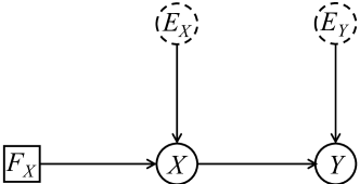
Figure 11: Simple SCM

In it, we have $X=f_{X}(E_{X})$, $Y=f_{Y}(X,E_{Y})$, with $E_{Y}\,\mbox{$\perp\!\!\!\perp$}\,X$. The deterministic structure of a SCM supports the introduction of potential responses (something that can not be done with a purely probabilistic DAG): $Y_{x}=f_{Y}(x,E_{Y})$. Then $X,Y_{0},Y_{1}$ are all functions of $(E_{X},E_{Y})$, and thus have a joint distribution entirely determined by that of $(E_{X},E_{Y})$. And given this joint distribution we can compute PC in (8). Likewise, given a more general SCM we can compute answers to CoE questions.

It would seem then that this approach bypasses the difficulties alluded to above. This, however, is illusory, since such a solution is available only when we have access to a fully specified SCM. As discussed in § 2.4 and § 6.1, there will be many distinct PSMs or SCMs consistent with a given probabilistic or augmented DAG model for the domain variables. Since the probabilistic structure is the most that we can learn from empirical data, we will never be able to choose between these distinct SCM versions of the problem. However, different SCMs will lead to different answers to the CoE questions we put to them. Thus for Figure 11, we have $\mbox{\rm PC}=\mbox{\rm P}(Y_{0}=0\mid Y_{1}=1)$, since $\mbox{\boldmath$Y$}\,\mbox{$\perp\!\!\!\perp$}\,X$, and this will depend on the dependence between $Y_{0}$ and $Y_{1}$ as embodied in the SCM. But because of the fundamental problem of causal inference, this dependence can never be identified from empirical data. So different SCMs inducing the same probabilistic structure, which are entirely indistinguishable empirically, will lead to different answers. When we allow for all possible such SCMs, we are led back to the interval bounds for PC discussed above.

8 Discussion

We have surveyed a variety of directed graphical models, with varying syntax (including or omitting error variables or regime indicators) and semantics (formal or informal, modelling probabilistic or causal situations). Different semantics are relevant to different rungs of the ladder of causation.

When presented with a simple DAG it may not be obvious how it is supposed to be interpreted, and there is an ever-present danger of misinterpretation, or of slipping too easily from one interpretation (e.g., purely probabilistic) to another (e.g., causal). This can largely be avoided by always using a simple DAG to model a probabilistic problem (on the first rung of the ladder), and an augmented DAG to model a causal problem (on the second rung). In both cases, the moralisation procedure provides the semantics whereby interpretive properties can be read off the graph.

DAGs such as SCMs, that involve, explicity or implicitly, error variables and functional relationships, can be used on all three rungs of the ladder. However they can not be identified empirically. For rungs one and two this is unimportant, and all equivalent versions, inducing the same underlying purely probabilistic DAG, will yield the same answers as obtainable from that underlying DAG. For rung 3, which addresses the probability of causation in an individual instance, only an approach based on SCMs is available. However, different but empirically indistinguishable SCMs now deliver different answers to the same causal question. Taking this into account we may have to be satisfied with an interval bound on the desired, but unidentifiable, probability of causation.

References

- Pearl (1988) Pearl, J. Probabilistic Reasoning in Intelligent Systems; Morgan Kaufmann Publishers: San Mateo, California, 1988.
- Lauritzen (1996) Lauritzen, S.L. Graphical Models; Oxford University Press, 1996.
- Cowell et al. (1999) Cowell, R.G.; Dawid, A.P.; Lauritzen, S.L.; Spiegelhalter, D.J. Probabilistic Networks and Expert Systems; Springer: New York, 1999.
- Pearl (2009) Pearl, J. Causality: Models, Reasoning and Inference, Second ed.; Cambridge University Press: Cambridge, 2009.
- Dawid and Evett (1997) Dawid, A.P.; Evett, I.W. Using a Graphical Method to Assist the Evaluation of Complicated Patterns of Evidence. Journal of Forensic Science 1997, 42, 226–231.
- Dawid (2002) Dawid, A.P. Influence Diagrams for Causal Modelling and Inference. International Statistical Review 2002, 70, 161–189. Corrigenda, ibid., 437.
- Dawid (2003) Dawid, A.P. Causal Inference Using Influence Diagrams: The Problem of Partial Compliance (with Discussion). In Proceedings of the Highly Structured Stochastic Systems; Green, P.J.; Hjort, N.L.; Richardson, S., Eds. Oxford University Press, 2003, pp. 45–81.
-
Dawid (2010a)
Dawid, A.P.
Beware of the DAG!
In Proceedings of the Proceedings of the NIPS 2008 Workshop on
Causality; Guyon, I.; Janzing, D.; Schölkopf, B., Eds., 2010, Vol. 6, Journal of Machine Learning Research Workshop and Conference Proceedings,
pp. 59–86.
http://tinyurl.com/33va7tm . - Dawid (2010b) Dawid, A.P. Seeing and Doing: The Pearlian Synthesis. In Heuristics, Probability and Causality: A Tribute to Judea Pearl; Dechter, R.; Geffner, H.; Halpern, J.Y., Eds.; College Publications: London, 2010.
- Dawid and Didelez (2010) Dawid, A.P.; Didelez, V. Identifying the Consequences of Dynamic Treatment Strategies: A Decision-Theoretic Overview. Statistical Surveys 2010, 4, 184--231.
- Geneletti and Dawid (2011) Geneletti, S.G.; Dawid, A.P. Defining and Identifying the Effect of Treatment on the Treated. In Causality in the Sciences; Illari, P.M.; Russo, F.; Williamson, J., Eds.; Oxford University Press, 2011; pp. 728--749.
-
Dawid (2015)
Dawid, A.P.
Statistical Causality from a Decision-Theoretic Perspective.
Annual Review of Statistics and its Application 2015,
2, 273--303.
DOI:10.1146/annurev-statistics-010814-020105. - Dawid et al. (2017) Dawid, A.P.; Musio, M.; Murtas, R. The Probability of Causation. Law, Probability and Risk 2017, 16, 163--179.
- Constantinou and Dawid (2017) Constantinou, P.; Dawid, A.P. Extended Conditional Independence and Applications in Causal Inference. Annals of Statistics 2017, 45, 2618--2653.
-
Dawid (2021)
Dawid, A.P.
Decision-Theoretic Foundations for Statistical Causality.
Journal of Causal Inference 2021, 9, 39--77.
DOI:10.1515/jci-2020-0008. -
Dawid (2022)
Dawid, A.P.
The Tale Wags the DAG. In Probabilistic and Causal Inference:
The Works of Judea Pearl; Dechter, R.; Geffner, H.; Halpern, J.Y., Eds.;
Association for Computing Machinery and Morgan & Claypool, 2022;
chapter 28, pp. 557--574.
DOI:10.1145/3501714.3501744. -
Dawid and Musio (2022)
Dawid, A.P.; Musio, M.
Effects of Causes and Causes of Effects.
Annual Review of Statistics and its Application 2022,
9, 261--287.
DOI:10.1146/annurev-statistics-070121-06112. -
Dawid et al. (2022)
Dawid, A.P.; Humphreys, M.; Musio, M.
Bounding Causes of Effects with Mediators.
Sociological Methods and Research 2022.
Online first, March, 2022, 29pp.
DOI:10.1177/00491241211036161. - Pearl and Mackenzie (2018) Pearl, J.; Mackenzie, D. The Book of Why; Basic Books: New York, 2018.
- Pearl (1986) Pearl, J. A Constraint--Propagation Approach to Probabilistic Reasoning. In Proceedings of the Uncertainty in Artificial Intelligence; Kanal, L.N.; Lemmer, J.F., Eds., Amsterdam, 1986; pp. 357--370.
- Verma and Pearl (1990) Verma, T.; Pearl, J. Causal Networks: Semantics and Expressiveness. In Proceedings of the Uncertainty in Artificial Intelligence 4; Shachter, R.D.; Levitt, T.S.; Kanal, L.N.; Lemmer, J.F., Eds., Amsterdam, 1990; pp. 69--76.
- Lauritzen et al. (1990) Lauritzen, S.L.; Dawid, A.P.; Larsen, B.N.; Leimer, H.G. Independence Properties of Directed Markov Fields. Networks 1990, 20, 491--505.
- Dawid (1979) Dawid, A.P. Conditional Independence in Statistical Theory (with Discussion). Journal of the Royal Statistical Society, Series B 1979, 41, 1--31.
- Frydenberg (1990) Frydenberg, M. The Chain Graph Markov Property. Scandinavian Journal of Statistics 1990, 17, 333--353.
- Verma and Pearl (1991) Verma, T.; Pearl, J. Equivalence and Synthesis of Causal Models. In Uncertainty in Artificial Intelligence 6; Bonissone, P.P.; Henrion, M.; Kanal, L.N.; Lemmer, J.F., Eds.; North-Holland: Amsterdam, 1991; pp. 255--268.
- Korzybski (1933) Korzybski, A. Science and Sanity: An Introduction to Non-Aristotelian Systems and General Semantics; International Non-Aristotelian Library Publishing Compan, 1933.
- Hernán and Robins (2006) Hernán, M.A.; Robins, J.M. Instruments for Causal Inference: An Epidemiologist’s Dream? Epidemiology 2006, 17, 360--372.
- Sadeghi and Soo (2023) Sadeghi, K.; Soo, T. Axiomatization of Interventional Probability Distributions. Research report, University College London, 2023. arXiv:2305.04479.
- Dawid (1980) Dawid, A.P. Conditional Independence for Statistical Operations. Annals of Statistics 1980, 8, 598--617.
- Constantinou and Dawid (2017) Constantinou, P.; Dawid, A.P. Extended Conditional Independence and Applications in Causal Inference. Annals of Statistics 2017, 45, 2618--2653.
- Holland (1986) Holland, P.W. Statistics and Causal Inference (with Discussion). Journal of the American Statistical Association 1986, 81, 945--970.
- Dawid (2007) Dawid, A.P. Counterfactuals, Hypotheticals and Potential Responses: A Philosophical Examination of Statistical Causality. In Causality and Probability in the Sciences; Russo, F.; Williamson, J., Eds.; College Publications: London, 2007; Vol. 5, Texts in Philosophy, pp. 503--32.
- Rubin (1974) Rubin, D.B. Estimating Causal Effects of Treatments in Randomized and Nonrandomized Studies. Journal of Educational Psychology 1974, 66, 688--701.
- Rubin (1978) Rubin, D.B. Bayesian Inference for Causal Effects: The Rôle of Randomization. Annals of Statistics 1978, 6, 34--68.
-
Dawid and Musio (2022)
Dawid, A.P.; Musio, M.
What Can Group Level Data Tell Us About Individual Causality? In Statistics in the Public Interest: In Memory of Stephen E. Fienberg;
Carriquiry, A.; Tanur, J.; Eddy, W., Eds.; Springer International Publishing,
2022; pp. 235--256.
DOI: 10.1007/978-3-030-75460-0_13.