DoorINet: A Deep-Learning Inertial Framework for Door-Mounted IoT Applications

Abstract

Many Internet of Things applications utilize low-cost, micro, electro-mechanical inertial sensors. A common task is orientation estimation. To tackle such a task, attitude and heading reference system algorithms are applied. Relying on the gyroscope readings, the accelerometer readings are used to update the attitude angles, and magnetometer measurements are utilized to update the heading angle. In indoor environments, magnetometers suffer from interference that degrades their performance. This mainly influences applications focused on estimating the heading angle like finding the heading angle of a closet or fridge door. To circumvent such situations, we propose DoorINet, an end-to-end deep-learning framework to calculate the heading angle from door-mounted, low-cost inertial sensors without using magnetometers. To evaluate our approach, we record a unique dataset containing 391 minutes of accelerometer and gyroscope measurements and corresponding ground-truth heading angle. We show that our proposed approach outperforms commonly used, model based approaches and data-driven methods. To enable reproducibility of our results and future research, both code and data are available at https://github.com/ansfl/DoorINet.

I Introduction

The Internet of Things (IoT) is essentially a network of devices that can collect information and connect to and communicate with each other without human interaction. Remote data storage and cloud computing allow automatic data analysis and decision-making capabilities. IoT-enabled devices combine multiple sensors such as inertial sensors, and can be a part of various applications such as motion capture and human activity recognition [1, 2, 3, 4], , sports applications [5, 6, 7, 8], health-related applications [9, 10, 11], pedestrian dead reckoning [12, 13, 14], and smart home applications [15, 16, 17].
Inertial measurement units (IMU) consist of three mutually orthogonal accelerometers and three gyroscopes aligned with the accelerometers. Additionally, there can be three orthogonal magnetometers aligned in the same direction as other sensors. Accelerometers provide the specific force vector, gyroscopes the angular rate vector, and the magnetometers the magnetic field vector. IMUs come in a wide range of performance grades intended for different applications. Though there is no universally agreed definition of high-, medium-, and low-grade IMUs, they can be grouped into several categories: marine, aviation, intermediate, tactical, and automotive [18]. Automotive grade is sometimes called consumer or commercial grade. The most affordable IMU sensors are usually built with micro electro-mechanical sensor (MEMS) technology, also making them small compared to mechanical IMUs. Miniaturized MEMS IMUs are widely used in consumer products, i.e., smartphones, IoT applications, and wearable devices.
In non-navigational applications (such as most IoT applications) inertial sensor readings are used as input to attitude and heading reference system (AHRS) algorithms that provide the orientation of a device; that is, the three Euler angles with respect to a fixed coordinate frame, which uniquely determine the orientation.
In model-based approaches the AHRS algorithm divides into two separate independent parts: orientation propagation from a gyroscope and readings followed by updates from accelerometer and magnetometer measurements. In nonlinear filtering approaches the attitude kinematic equations are treated as the system model, and the accelerometer and magnetometer observations are processed in the measurement model to update the state and propagate the error-state covariance matrix [19]. Another commonly used approach is complementary filtering, which combines compensated gyroscope measurements with gain-multiplied measurements from accelerometers and magnetometers [20, 21]
In learning-based approaches, IMU readings are fed directly into the deep-learning algorithm to provide attitude and heading estimation [22]. Alternatively, a deep-learning algorithm can be used for denoising inertial measurements, and attitude estimation is obtained using an integrated processed ”noise-free” signal like in [23]. Hybrid approaches try to combine the best of model and learning approaches. For example, the deep attitude estimator [24, 25, 26] uses a deep-learning model to calculate gain for the complementary filter algorithm structure.
Indoor environments are full of electromagnetic fields, resulting in constant and time varying influence on magnetometer readings. This is even more relevant in specific industrial buildings with high levels of magnetic field where the heading angle estimation accuracy degrades.
In this paper we introduce and address the problem of door mounted IMUs. Here, the goal is to determine the opening angle of a door. This information may be utilized in several IoT applications such as smart homes, smart offices, or building management. To cope with low magnetometer performance in an indoor enthronement, we propose DoorINet, a deep-learning, end-to-end framework for estimating the heading angle of door-mounted IMU using only accelerometers and gyroscopes. Two versions of DoorINet are examined: AG-DoorINet that takes accelerometer and gyroscope measurements, and G-DoorINet that takes only gyroscope readings.
To evaluate our proposed approaches we re-record a unique dataset using Xsens DOT IMUs mounted on three different doors, resulting in 391 minutes of recorded inertial data and accurate headings obtained from a higher grade Memsense IMU. We compare our approach with two model-based and three learning-based AHRS approaches and show that ours outperform the rest on a real-life scenario of an inner door over 90 minutes. Our deep-learning framework is able to generalize over different error parameters of different IMU sensors, and it is able to correctly calculate the heading angle.
The contributions of this paper are as follows:

1. Derivation of two end-to-end networks capable of accurately regressing the heading angle of a door-mounted inertial sensors using only accelerometer and gyroscope readings.

2. Recording of a unique dataset containing 391 minutes of accelerometer and gyroscope measurements and corresponding ground-truth (GT) heading angle.

3. Ensuring reproducibility of our results and encouraging future research by making the code and dataset available at this GitHub repository.

The rest of the paper is organized as follows: Section II introduces model-based approaches for heading estimation. Section III describes our proposed learning approach for heading determination. Section IV explains our dataset collection setup while Section V describes post-processing procedures. Section VI shows the experimental results and Section VII concludes this work.

II Model-Based AHRS Algorithms

There are several model-based AHRS algorithms that estimate the attitude and heading of a platform. As this work focuses only on the heading angle, we briefly review the direct integration approach and the Madgwick complementary filtering approach.

II-A Direct Integration

Gyroscopes measure angular velocity, that is, the change of angle with respect to time. Assuming the gyroscope’s sensitive axis is aligned with the gravity direction, the heading angle $\psi$ can be found by integrating the angular velocity $w$ component parallel to the gravity direction:

$$\psi(t)=\psi_{0}+\int_{t}w_{t}\,dt\,$$ (1)

where $\psi_{0}$ is the initial heading angle. This approach does not take into account error factors in the gyroscope sensor and alignment errors and therefore is considered less accurate than AHRS methods.

II-B Madgwick Filter

Madgwick first proposed an orientation filter for inertial and inertial/magnetic sensor arrays in [27], and later its extended version [28]. We follow a version of the Madgwick algorithm as presented in chapter 7 of [20]. This algorithm functions as a complementary filter that combines compensated gyroscope measurements with filtered measurements from the accelerometer with a frequency determined by the gain.
The orientation is obtained from integration of the quaternion derivative describing the rate of change of orientation of the earth frame $E$ relative to the sensor frame $S$, by

$$\prescript{S}{E}{\boldsymbol{\mathrm{q}}}=\int_{t}\prescript{S}{E}{\dot{\boldsymbol{\mathrm{q}}}}\,dt,$$ (2)

where $\prescript{S}{E}{\boldsymbol{\mathrm{q}}_{\omega,t}}$ is the unnormalized orientation and $\prescript{S}{E}{\dot{\boldsymbol{\mathrm{q}}}_{\omega,t}}$ is the quaternion derivative defined by

$$\prescript{S}{E}{\dot{\boldsymbol{q}}}=\frac{1}{2}\prescript{S}{E}{\hat{\boldsymbol{\mathrm{q}}}}\otimes\begin{matrix}{[0,(\boldsymbol{\mathrm{\omega}}^{\prime}+Ke)^{T}]}\end{matrix},$$ (3)

where $\prescript{S}{E}{\hat{\boldsymbol{\mathrm{q}}}}$ is a normalized orientation in a quaternion form, $\otimes$ is the quaternion product, $\boldsymbol{\mathrm{\omega}}^{\prime}$ is the gyroscope measurement vector, $K$ is the algorithm gain, and $e$ is an error term.
The initial value of $\prescript{S}{E}{\hat{\boldsymbol{\mathrm{q}}}}$ is assumed to be an identity quaternion, and the algorithm to determine the gain K is

$$K=\begin{cases}K_{norm}+\frac{t_{init}-t}{t_{init}}(K_{init}-K_{norm}),&\text{if }t<t_{init}\\ K_{norm}&\text{else}\end{cases}$$ (4)

where $K_{init}$ is the initial large value of gain, $K_{norm}$ is the value intended for normal operation, and $t_{init}$ is the initialization period.
The error term used in (3) is defined by

$$e=\begin{cases}e_{f},&\text{else if }||\boldsymbol{\mathrm{f}}||>0,\\ \begin{bmatrix}0&0&0\end{bmatrix}^{T}&\text{else},\end{cases}$$ (5)

where $\boldsymbol{\mathrm{f}}$ is the specific force measurement vector, and $e_{f}$ is the accelerometer error factor defined as

$$\boldsymbol{e}_{f}=\hat{\boldsymbol{\mathrm{f}}}\times\begin{bmatrix}2q_{x}q_{y}-2q_{w}q_{z}\\ 2q^{2}_{w}-1+2q^{2}_{y}\\ 2q_{y}q_{z}-2q_{w}q_{x}\end{bmatrix},\hat{\boldsymbol{\mathrm{f}}}=\frac{\boldsymbol{\mathrm{f}}}{||\boldsymbol{\mathrm{f}}||}$$ (6)

where $\boldsymbol{\mathrm{f}}$ is the specific force vector measured by the accelerometer, and $q_{w}$, $q_{x}$, $q_{y}$, $q_{z}$ are elements of $\prescript{S}{E}{\hat{\boldsymbol{\mathrm{q}}}}$.
Additional features of this algorithm are designed to address various challenges (sensor conditioning, gyroscope bias compensation, linear acceleration rejection, etc.) and are not described in this paper.

III Proposed Approach

When working with IoT applications it is crucial to ensure the heading accuracy in longer time durations. Current AHRS algorithms either require fine-tuning to the current scenario to provide valid results, or are simply unable to provide them as low-cost inertial sensors are employed.
In this work we propose DoorINet, a deep-learning inertial framework for door-mounted IoT applications. To that end, we design a deep-learning architecture fed by accelerometer and gyroscope readings to regress the heading angle as presented in Figure 1. The advantages of our approach are twofold:

1. No fine-tuning or weight parameters are required (in contrast to model-based approaches)

2. Using deep-learning algorithms allows leveraging its well-known properties like noise reduction, the ability to cope with nonlinearities in the data, and the potential ability to generalize over different sensor error parameters.

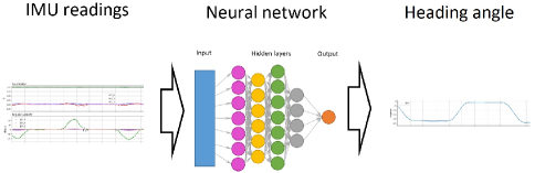
Figure 1: Proposed data-driven approach.

As IoT applications are considered, we focused our design on relatively shallow architectures allowing their implementation for real-time settings. Two types of networks are proposed, differing in their structure and input, as addressed in the next section.

III-A Gyroscope-Only DoorINet Architecture (G-DoorINet)

Our network comprises bidirectional gated recurrent units (BiGRU)—a type of recurrent layers—and fully connected (FC) layers. A recurrent layer consists of a hidden state $\boldsymbol{\mathrm{h}}$ and an optional output $\boldsymbol{y}$ that operates on a variable-length sequence $\mathrm{\boldsymbol{x}}=(x_{1},...,x_{T})$. At each time step t, the hidden state $\boldsymbol{\mathrm{h}}_{\langle t\rangle}$ of the layer is updated by

$$\boldsymbol{\mathrm{h}}_{\langle t\rangle}=f(\boldsymbol{\mathrm{h}}_{\langle t-1\rangle},\boldsymbol{\mathrm{x}}_{t}),$$ (7)

where $f$ is a non-linear activation function.
Bidirectional recurrent layers were introduced in [29] and they connect hidden states of two recurrent layers processing an input sequence in both forward and backward directions to the same output.
GRU layers are a specific type of RNN layer that was first suggested in [30] for natural language processing applications. GRU layers have two main gates allowing them to adaptively remember and forget information. The reset gate $r_{j}$ is computed by

$$r_{j}=\sigma([\boldsymbol{\mathrm{W}}_{r}\boldsymbol{\mathrm{x}}]_{j}+[\boldsymbol{\mathrm{U}}_{r}\boldsymbol{\mathrm{h}}_{\langle t-1\rangle}]_{j}),$$ (8)

where $\sigma$ is the logistic sigmoid function, and $[.]_{j}$ denotes the $j$-th element of a vector. $\boldsymbol{\mathrm{x}}$ and $\boldsymbol{\mathrm{h}}_{t-1}$ are the input and the previous hidden state, respectively. $\boldsymbol{\mathrm{W}}_{r}$ and $\boldsymbol{\mathrm{U}}_{r}$ are weight matrices that are learned.
The update gate $z_{j}$ is computed by

$$z_{j}=\sigma([\boldsymbol{\mathrm{W}}_{z}\boldsymbol{\mathrm{x}}]_{j}+[\boldsymbol{\mathrm{U}}_{z}\boldsymbol{\mathrm{h}}_{\langle t-1\rangle}]_{j}).$$ (9)

The actual activation of the proposed unit $h_{j}$ is then computed by

$$h_{j}^{\langle t\rangle}=z_{j}h_{j}^{\langle t-1\rangle}+(1-z_{j})\tilde{h}_{j}^{\langle t\rangle},$$ (10)

where

$$\tilde{h}_{j}^{\langle t\rangle}=\phi([\boldsymbol{\mathrm{Wx}}]_{j}+[\boldsymbol{U}(\boldsymbol{\mathrm{r}}\odot\boldsymbol{\mathrm{h}}_{\langle t-1\rangle}])$$ (11)

where $\odot$ is an element-wise (Hadamard) product.
When the reset gate is close to zero, the hidden state is forced to ignore the previous hidden state and is reset with the current input only. This allows the hidden state to drop any information that is found to be irrelevant later in the future, allowing a more compact representation. On the other hand, the update gate controls how much information from the previous hidden state carries over to the current hidden state.

In addition to BiGRU layers we employ fully connected (FC) layers, which were first introduced in [31], and calculate vector-matrix multiplication $\boldsymbol{\mathrm{x}}\times\boldsymbol{\mathrm{W}}$, where $\boldsymbol{\mathrm{x}}$ is the input vector and $\boldsymbol{\mathrm{W}}$ is the weight matrix. An activation function tanh is applied between fully connected layers element-wise and defined as

$$tanh(\boldsymbol{\mathrm{x}}_{j})=\frac{exp(\boldsymbol{\mathrm{x}}_{j})-exp(-\boldsymbol{\mathrm{x}}_{j})}{exp(\boldsymbol{\mathrm{x}}_{j})-exp(-\boldsymbol{\mathrm{x}}_{j})}$$ (12)

where $\boldsymbol{\mathrm{x}}_{j}$ is a $j$-th element of a $tanh$ input.
Our gyroscope-only DoorINet (G-DoorINet) architecture consists of consequent bi-directional GRU (BiGRU) layers that feed on gyroscope measurements and then FC layers as presented in Figure 2:

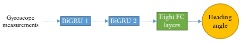
Figure 2: G-DoorINet network architecture using only gyroscope measurements.

In Table I we give G-DoorINet network parameters including input and output sizes.

TABLE I: G-DoorINet network parameters.

Layer	Input size	Output size	Additional
BiGRU 1	3	64	bidirectional
BiGRU 2	128	128	bidirectional
FC 1	5120	2560	Dropout p=0.2; Tanh
FC 2	2560	512	Tanh
FC 3	512	128	Tanh
FC 4	128	32	Tanh
FC 5	32	16	Tanh
FC 6	16	8	Tanh
FC 7	8	4	Tanh
FC 8	4	1	-

III-B Accelerometer and Gyroscope DoorINet Architecture (AG-DoorINet)

The accelerometer and gyroscope model (AG-DoorINet) consists of two sets of stacked, bi-directional GRU (BiGRU) layers that feed on accelerometer and gyroscope data (making it a multi-head neural network), whose outputs are fed to another GRU layer and FC layers afterwards, as illustrated in Figure 3).

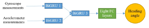
Figure 3: AG-DoorINet network architecture using accelerometer and gyroscope measurements.

Table II presents the AG-DoorINet network parameters including input and output sizes.

TABLE II: AG-DoorINet network parameters.

Layer	Input size	Output size	Additional
BiGRU 1	3	64	Bidirectional; stacked layers=3
BiGRU 2	3	64	Bidirectional; stacked layers=3
BiGRU 3	256	256	Bidirectional; stacked layers=2
FC 1	10240	2560	Dropout p=0.2; Tanh
FC 2	2560	512	Dropout p=0.2; Tanh
FC 3	512	128	Tanh
FC 4	128	32	Tanh
FC 5	32	16	Tanh
FC 6	16	8	Tanh
FC 7	8	4	Tanh
FC 8	4	1	-

IV Dataset generation

Our dataset was recorded using two types of IMUs: Memsense MS-IMU3025 [32] and Movella Xsens DOT [33]. The Memsense MS-IMU3025 was used to generate the ground-truth (GT) readings. This IMU has a gyroscope bias instability of 0.8°/h over the axis of interest Z and was recorded at 250Hz. The Movella Xsens DOT IMUs were used as units under test. It has a gyroscope bias instability of 10°/h over the axis of interest Z and was recorded at 120Hz.
Three experimental setups were designed and implemented to generate raw inertial data. The setups differ in the number of inertial sensors used and their location on the door surface:

1. Setup 1 Two IMUs—the Memsense and a single DOT—were placed on the door surface next to the handle, as shown in Figure 4a.

2. Setup 2 is similar to Setup 1, but a different DOT sensor was used, and sensors were placed at three different locations consecutively: first next to the door handle, then in the middle of the door, and finally next to the door hinge, to test the influence of sensor position on recorded data and results.

3. Setup 3 Consists of the Memsense and ten DOTs placed on a different door (than in Setup 1 and 2) in different positions at the same time. Eight DOTs were placed near the door handle, one in the middle, and one near the door hinge. This setup allowed recording more data in each experiment, and is shown in Figure 4b

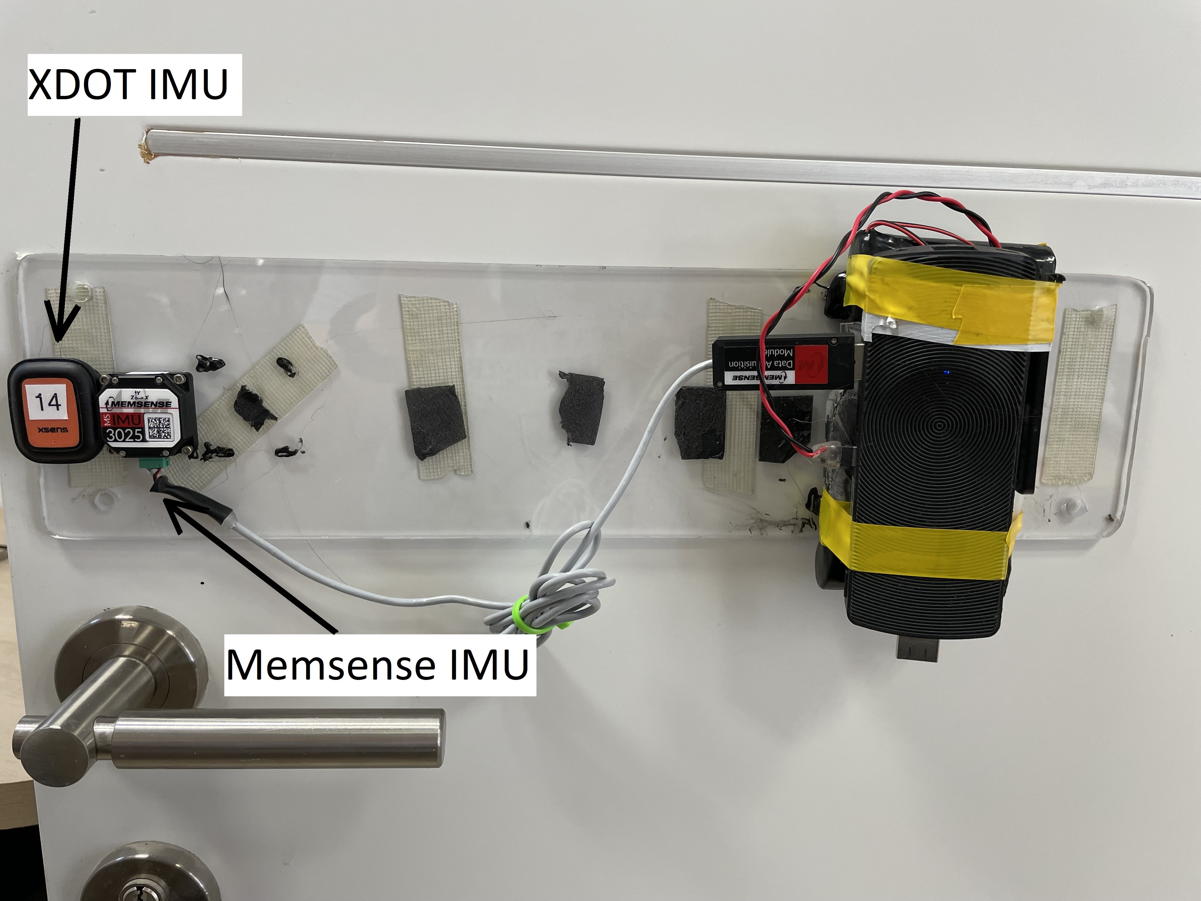
(a) Setups 1 and 2

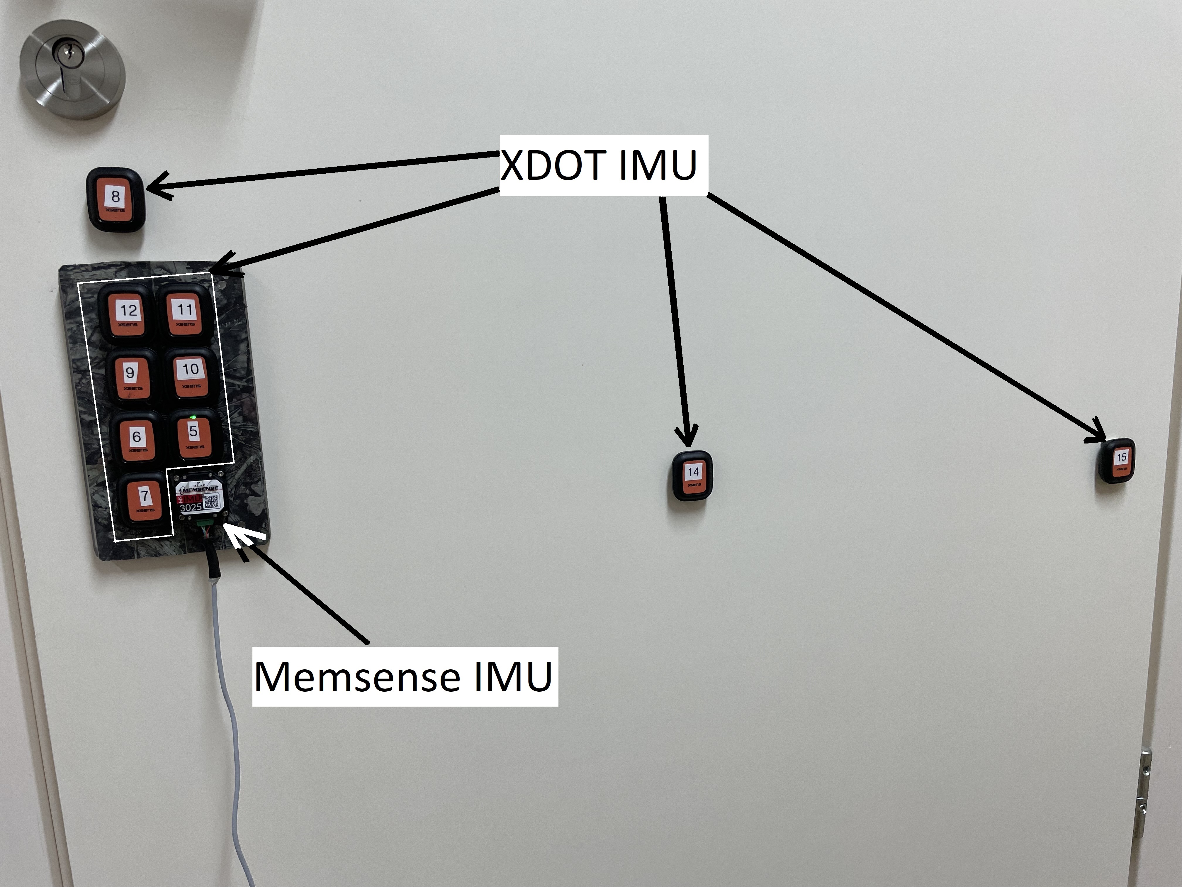
(b) Setup 3

Figure 4: Experimental setups used for dataset generation: DOT IMUs generated raw IMU readings and Memsense IMU generated the ground truth.

Each recording session comprised several experiments with a duration of 60-120 seconds each. Each experiment consisted of a series (usually 9-11) of openings and closings of the door at a normal speed (like a person would usually open and close the door) to a predetermined angle. Each opening and each closing was followed by a stop (an absence of movement) for 2-5 seconds. After each opening the door was closed shut.
Below we elaborate on the specific recording time and setup of the train, validation, and test datasets.

IV-A Train and validation datasets

The training dataset comprising IMU data recorded in Sessions 1, 2, and 3 is explained below.

IV-A1 Session 1

The lab door at the Israel Oceanographic and Limnological Research Institute on Tel Shikmona, Haifa, Israel, with experimental Setup 1.
In this session ten experiments were recorded in total to examine the overall performance and data processing. In each experiment the door was opened to the same angle and closed shut ten times. The approximate angles for the main experiments were in the order of recording: 15°, 30°, 45°, 60°, 75°, 90°. In four test experiments the door was opened and closed three times. The approximate angles for those experiments were 15°, 45°, and 90°. An example of the DOT raw data of the accelerometers and gyroscopes as well as the GT heading is presented in Figure 5.

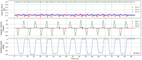
Figure 5: An example of data recorded in Session 1.

IV-A2 Session 2

The Autonomous Navigation and Sensor Fusion Lab door at the University of Haifa, Israel, with experimental Setup 2.
In this session three experiments were recorded according to the Setup 2. An additional experiment was recorded in a distant location from the door hinge with IMUs rotated 90°clockwise. At each location two experiments were recorded with a total of eight experiments. In each experiment the door was opened to a predefined angle and closed shut five times. The approximate chosen angles for the experiments were 32°and 64°.
An example of the DOT raw data of the accelerometers and gyroscopes as well as the GT heading is presented in Figure 6.

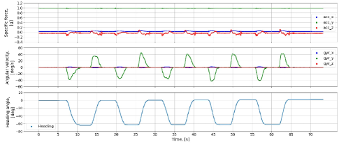
Figure 6: An example of data recorded in Session 2.

IV-A3 Session 3

The Autonomous Navigation and Sensor Fusion Lab door at the University of Haifa, Israel, with experimental Setup 3.
In this session eight experiments were recorded in total. In each, the door was opened to a predefined angle and closed shut, 10-11 times. In the last three experiments the door was opened to 90° at different speeds: relatively slow, medium, and fast.
An example of the DOT raw data of the accelerometers and gyroscopes as well as the GT heading is presented in Figure 7.

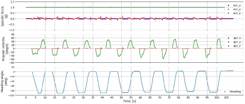
Figure 7: An example of data recorded in Session 3.

IV-B Test dataset

The test dataset was recorded last, during Session 3. This was a scenario of using the door for 90 minutes of non-stop recording. The door was opened and closed at will, with several people walking in and out of the internal laboratory room. No specified angle or pattern was used. The door was opened and closed 31 times during this period.

IV-C Dataset summary

The summary of the dataset used for training, validation, and testing is presented in Table III. In total the train dataset has a duration of 95.3 minutes and the validation dataset is 23.8 minutes in length. We used the following notation for the inertial sensor locations: EP1 = close to the door handle, EP2 = in the middle of the door, and EP3 = close to the door hinge. The test dataset has a duration of 271.9 minutes. It also includes DOT #12 recordings, which are not present in the train and validation datasets.

TABLE III: Dataset summary showing the description and duration of each experiment. In total, the dataset includes 391 minutes of recorded data.

Setup #	Duration, s	#DOT IMUs	IMU sensors location, Experiment description	Used in dataset
1	86.9	1	EP1, 5 angles	train & val
1	92.9	1	EP1, 6 angles	train & val
1	106.3	1	EP1, 6 angles	train & val
1	113.2	1	EP1, 6 angles	train & val
1	118.9	1	EP1, 6 angles	train & val
2	63.2	1	EP1, 6 angles	train & val
2	71.5	1	EP1, 6 angles	train & val
3	868.1	8	EP1, EP2, EP3, 1 angle	train & val
3	870.6	8	EP1, EP2, EP3, 1 angle	train & val
3	766.1	8	EP1, EP2, EP3, 1 angle	train & val
3	789.4	8	EP1, EP2, EP3, 1 angle	train & val
3	697.4	8	EP1, EP2, EP3, 1 angle	train & val
3	645.1	8	EP1, EP2, EP3, Fast speed	train & val
3	828.4	8	EP1, EP2, EP3, Medium speed	train & val
3	1028.7	8	EP1, EP2, EP3, Slow speed	train & val
3	16312.5	3	EP1, EP2, EP3, Test scenario	test

V Data processing, model implementation, and training

V-A Preprocessing steps: train dataset

To improve the accuracy, two steps were applied to the train and validation datasets.
1) Gyro calibration: First order stationary gyro calibration was done for both DOT and Memsense IMUs while the door was shut. The calibration window was 30 to 50 data points. These estimated biases, in each axis, were subtracted from gyroscope readings.
2) Enforcing zero drift: Zero drift was enforced for each closing of the door for both DOT and Memsense IMUs. As we know that in each experiment the door was shut for two to five seconds between openings, we applied an algorithm that detects periods of the door being shut, so the starting angle is set to zero at the moment the door is shut closed. Figure 8 shows an example of the Memsense IMU with and without enforcing zero drift.

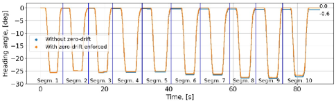
Figure 8: Setting sensor drift to zero for training data. Note the values of the final sensor drift for processed and unprocessed data on the left of the plot.

V-B Preprocessing steps: test dataset

For the GT heading angle (generated by Memsense IMU3025 IMU) a modified ”thresholded” version of Madgwick algorithm was introduced. At each time frame it compares the gyroscope vector norm with a predefined threshold, and if the vector norm is below the threshold, the algorithm assumes that there is no movement at that specific time frame and keeps the last value of the heading angle. As a consequence, the GT heading was altered to reflect the actual conditions of the shut door periods as shown in Figure 9.

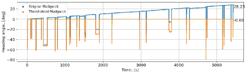
Figure 9: Raw (blue) and threshold-processed GT (orange) heading angles for the test dataset.

V-C Model implementation and training

The approach for training includes generating training data from lower-grade IMUs, recorded simultaneously, with the heading GT from a higher grade IMU as illustrated in Figure 10. In this setting the deep-learning model is able to generalize over different sensor parameters and behavior.

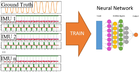
Figure 10: Proposed training approach with heading GT from a higher grade IMU.

Model-based algorithms were implemented in the Python programming language; the Madgwick algorithm was already implemented in imufusion Python package (https://github.com/xioTechnologies/Fusion). All our modifications of Madgwick algorithm were implemented as additions to the implementation mentioned above.
Our DoorINet deep-learning models were implemented in the PyTorch framework version 2.1.0+cu116 and were trained on the train dataset using a validation dataset for monitoring the training process using a back-propagation algorithm. Weights of our networks were initialized using the Xavier uniform initialization scheme [34]. The hardware used for training was an ASUS TUF Gaming A17 laptop with AMD Ryzen 7 4800H CPU, 16GB RAM, and Nvidia GeForce GTX 1660 Ti GPU. We used a Huber loss function (designed for regression problems) with default parameters, described as

$$HuberLoss(\boldsymbol{\mathrm{Y}},\boldsymbol{\mathrm{\hat{Y}}})=mean(l_{1},...,l_{n})$$ (13)

where $\boldsymbol{\mathrm{Y}}$ is the ground-truth vector, $\boldsymbol{\mathrm{\hat{Y}}}$ is the model output vector, $n$ is the number of model outputs, and $l_{i}$ is calculated as a function of $i$-th elements $y_{i}$ of the ground truth and $\hat{y}_{i}$ of the model output by

$$l_{i}=\begin{cases}0.5(y_{i}-\hat{y}_{i})^{2},&\text{if }|y_{i}-\hat{y}_{i}|<1,\\ (|y_{i}-\hat{y}_{i}|-0.5),&\text{otherwise}.\end{cases}$$ (14)

Training was performed over 150 epochs using the AdamW optimizer and ReduceOnPlateau scheduler with an initial learning rate of 1e-3, reducing the learning rate by two after waiting for three epochs of the loss value dropping less than 0.01. The history of loss values during the training phase are presented in Figure 11.

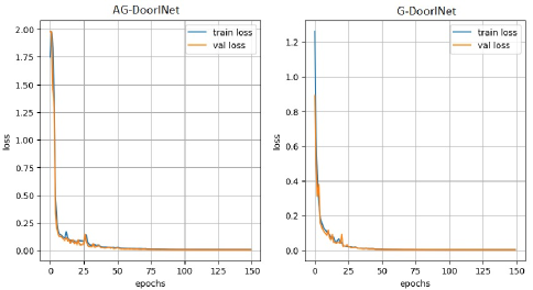
Figure 11: Train and validation losses for AG-DoorINet (left) and G-DoorINet (right).

For our results to be as reproducible as possible we introduced seed value as a hyperparameter for the training procedure. The seed value initializes the pseudorandom number generator in PyTorch and NumPy libraries, so every time a generator is used to generate a number (i.e., during the initialization phase), it does so in a deterministic fashion. Therefore, a training optimization process starts from a fixed point on a loss hypersurface, ensuring convergence to the same values on every run.
We performed training with ten randomly chosen seed values. Results presented in this paper were obtained with seed values that produce results close to the average, which were seed value 700 for AG-DoorINet and 35 for G-DoorINet.

VI Experimental results

VI-A Metrics

Several metrics were used to measure performance of different models:

• Root mean squared error (RMSE) is the square root of the sum of squares of difference between the processed heading GT, $\boldsymbol{\mathrm{Y}}$, and the estimated heading, $\boldsymbol{\mathrm{\hat{Y}}}$:

  $$RMSE=\sqrt{\frac{1}{n}\sum_{i=1}^{n}(y_{i}-\hat{y}_{i})}$$ (15)

  where $n$ is a number of model outputs.

• Last point difference (LPD) between the absolute value of the difference of the sum of GT heading to its estimate:

  $$LPD=\bigg{|}\sum_{i=1}^{n}y_{i}-\sum_{i=1}^{n}\hat{y}_{i}\bigg{|}.$$ (16)

• Maximum absolute difference (MAD) is defined as the maximum value of the LPD over all instances during the evaluation:

  $$MAD=\max_{i}\bigg{\{}\bigg{|}\sum_{i=1}^{n}y_{i}-\sum_{i=1}^{n}\hat{y}_{i}\bigg{|}\bigg{\}}.$$ (17)

VI-B Competitive approaches

There exist a significant number of data-driven models for orientation estimation. Most of them solve a 3D estimation problem, which in our case is superficial as we are focused only on the heading angle estimation. We compare our approaches to five other methods. Two are model-based approaches: the direct integration approach, as described in Section II-A, and the Madgwick filter, presented in Section II-B. In addition, three data-driven approaches were implemented for comparison with our approach:

VI-B1 Deep Attitude Estimator (DAE) [25]

combines both deep learning and a model-based backbone. It uses accelerometers and gyroscopes as input. The underlying idea of this approach is to estimate gain for a complementary filter algorithm using a neural network.

VI-B2 Quaternion Model A [22]

consists of convolution layers, bi-directional LSTM layers, max-pooling, and fully connected layers, and can work with inertial sensors with different sampling rates. The goal of the paper was to achieve a real-time accurate three-dimensional attitude estimation using accelerometer and gyroscope readings.

VI-B3 LGC-Net [23]

performs denoising of IMU readings of low-cost, MEMS-based inertial sensors and contains special kinds of layers: depthwise separable convolution [35] and large kernel attention [36] layers. The authors aimed to obtain clean gyroscope readings free from noise and bias, so the orientation could be obtained by directly integrating it.
We implemented the LGC-Net model based on its description in [23] and trained it on our dataset. We used the HuberLoss loss function instead of the Log-cosh loss function implemented in the [23].

VI-C Results

As described in Table III, the test dataset includes recordings of DOT #12 that were not used in the train and validation dataset, IMU #14 that was used in Session 1 to generate 7.2% of the data used for training and validation, and IMU #5 that was used in Session 3 to generate 11.5% of the training/validation data sets. The following figures presenting the results are divided into two parts. The top plot shows all of the examined model outputs and heading GT, while the bottom plot shows the heading error of each model.

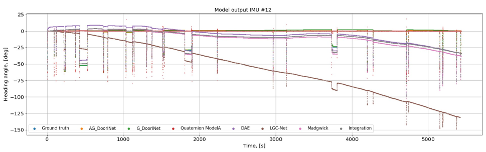
Figure 12: Estimated heading angle obtained by seven different approaches and heading GT for the test dataset containing IMU #12 readings.

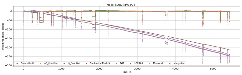
Figure 13: Estimated heading angle obtained by seven different approaches and heading GT for the test dataset containing IMU #14 readings.

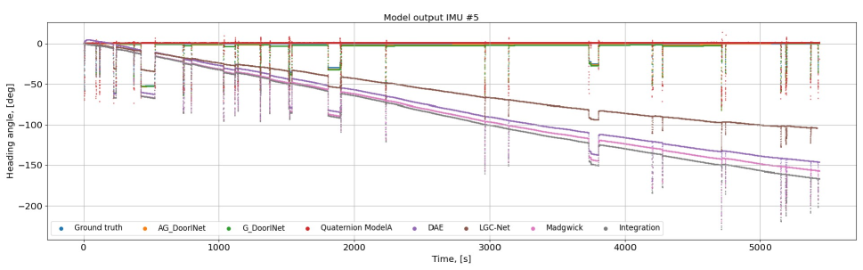
Figure 14: Estimated heading angle obtained by seven different approaches and heading GT for the test dataset containing IMU #5 readings.

Figure 12 presents the estimated heading angle of our two approaches and five other approaches as described in the previous section. The heading was estimated using the test dataset of DOT #12, which was not present in the train dataset. As presented in the Figure 12, all of the tested algorithms perform worse than the proposed DoorINet models, and their performance becomes worse with time (the difference becomes bigger). The figure also shows that the Quaternion ModelA fails to calculate the correct angle for the door opening. Both of our approaches obtained the best performance where AG-DoorINet has a minimum RMSE of 1.24 degrees.
In the same manner, Figure 13 presents the results of the test data recorded with the DOT IMU #14. This IMU was previously used in recording Session 1, generating 7.2% of the training and validation data. The Madgwick algorithm is comparable to the gyroscope integration approach. Both of our models perform better than others, where AG-DoorINet achieves the minimum RMSE of 1.03 degrees.
Figure 14 presents the performance of all the test data recorded by DOT IMU #5. This IMU was used in Session 3, and generated 11.5% of all the training and validation data. The DAE hybrid approach improved the result given by gyroscope integration and Madgwick algorithms, but the DoorINet model has better results and lower RMSE values (as low as 1.42 degrees for AG-DoorINet).

VI-D Summary

A summary of all the results described above is presented in Table IV.

TABLE IV: Summary of the results obtained using three different test datasets.

Model	RMSE [deg]	LPD [deg]	MAD [deg]
DOT IMU #12 (never used for producing training data)
Madgwick algorithm	14.25	38.09	40.47
Gyroscope integration	12.23	34.00	36.68
DAE	11.78	38.09	40.47
LGC-Net (our implementation)	67.34	130.87	130.91
Quaternion Model A	10.72	19.67	65.48
AG-DoorINet (ours)	1.24	0.02	7.14
G-DoorINet (ours)	1.35	0.02	7.25
DOT IMU #14 (used to produce 7.2% of training data)
Madgwick algorithm	132.28	246.34	247.87
Gyroscope integration	133.65	248.89	250.69
DAE	125.83	239.22	240.74
LGC-Net (our implementation)	115.48	211.47	211.47
Quaternion Model A	10.44	18.81	67.76
AG-DoorINet (our)	1.03	0.02	6.26
G-DoorINet (our)	4.62	0.02	9.16
DOT IMU #5 (used to produce 11.5% of training data)
Madgwick algorithm	96.05	156.96	160.89
Gyroscope integration	100.78	166.33	170.48
DAE	89.62	146.09	150.12
LGC-Net (our implementation)	65.20	103.87	104.01
Quaternion Model A	10.84	18.92	64.34
AG-DoorINet (our)	1.42	0.02	11.46
G-DoorINet (our)	1.93	0.02	12.45

All the tested algorithms operate only with accelerometer and gyroscope readings. Potentially, the Madgwick algorithm could improve its performance by incorporating magnetic readings, but that would require additional fine tuning and may not be suitable in environments with strong and changing magnetic interference.
Our accelerometer and gyroscope AG-DoorINet model shows better performance than the gyroscope-only G-DoorINet on all the metrics and test data, which indicates that the accelerometes measurements contribute to the heading accuracy. When the door is used in an ordinary fashion, acceleration naturally takes place as a human cannot open or close the door without accelerating it. Therefore, this additional information about the movement embedded in the accelerometer readings helps in improving the heading angle calculations.
Although all learning approaches were trained on the same training set, ours performed better as it was designed specifically for door dynamics, which is limited compared to the other approaches designed to handle general attitude and heading setups.

VII Conclusion

In this work we derived and presented DoorINet; a deep-learning, end-to-end framework to estimate the angle of an opening door using only low-cost inertial sensors. We introduced two models: AG-DoorINet that uses accelerometer and gyroscope IMU readings, and G-DoorINet that uses only gyroscope readings. To evaluate our approaches we recorded a unique dataset using ten low-cost sensors and a corresponding GT heading angle obtained using a higher grade sensor. The train and validation dataset consists of 119 minutes of IMU recordings while the test dataset has 272 minutes of IMU recordings. Included in the test set is a real-world scenario of over 90 minutes duration of a non-stop recording of opening/closing a door.
We demonstrated the strength of our proposed approach by comparing it with five model- and learning-based approaches. Our AG-DoorINet approach obtained the best performance (RMSE, MAD, and LPD) across all examined scenarios. Our deep-learning framework was able to generalize over different error parameters of different inertial sensors, and maintained performance for a long duration of 90 minutes.
G-DoorINet also outperformed all other approaches yet obtained lower performance compared to AG-DoorINet. Thus, the accelerometer measurements contribute in improving the overall performance, providing additional information about the door motion.
DoorINet is suitable for different smart home and office applications; for example, smart office, home office, or building management.
In addition, DoorINet can be implemented on any other AHRS application. In future work, we aim to extend DoorINet to include estimation of the roll and pitch angles.

References

- [1] O. D. Lara and M. A. Labrador, “A survey on human activity recognition using wearable sensors,” IEEE Communications Surveys & Tutorials, vol. 15, no. 3, pp. 1192–1209, 2013.
- [2] L. Pei, R. Guinness, R. Chen, J. Liu, H. Kuusniemi, Y. Chen, L. Chen, and J. Kaistinen, “Human behavior cognition using smartphone sensors,” Sensors, vol. 13, no. 2, pp. 1402–1424, 2013. [Online]. Available: https://www.mdpi.com/1424-8220/13/2/1402
- [3] M. Abdel-Basset, H. Hawash, V. Chang, R. K. Chakrabortty, and M. Ryan, “Deep learning for heterogeneous human activity recognition in complex IoT applications,” IEEE Internet of Things Journal, vol. 9, no. 8, pp. 5653–5665, 2022.
- [4] W. Zhuang, Y. Chen, J. Su, B. Wang, and C. Gao, “Design of human activity recognition algorithms based on a single wearable IMU sensor,” International Journal of Sensor Networks, vol. 30, no. 3, pp. 193–206, 2019. [Online]. Available: https://www.inderscienceonline.com/doi/abs/10.1504/IJSNET.2019.100218
- [5] J. M. Santos-Gago, M. Ramos-Merino, S. Vallarades-Rodriguez, L. M. Álvarez Sabucedo, M. J. Fernández-Iglesias, and J. L. García-Soidán, “Innovative use of wrist-worn wearable devices in the sports domain: A systematic review,” Electronics, vol. 8, no. 11, 2019. [Online]. Available: https://www.mdpi.com/2079-9292/8/11/1257
- [6] Y. Wang, M. Chen, X. Wang, R. H. M. Chan, and W. J. Li, “Iot for next-generation racket sports training,” IEEE Internet of Things Journal, vol. 5, no. 6, pp. 4558–4566, 2018.
- [7] M. Wu, M. Fan, Y. Hu, R. Wang, Y. Wang, Y. Li, S. Wu, and G. Xia, “A real-time tennis level evaluation and strokes classification system based on the internet of things,” Internet of Things, vol. 17, p. 100494, 2022. [Online]. Available: https://www.sciencedirect.com/science/article/pii/S2542660521001335
- [8] I. Ghosh, S. Ramasamy Ramamurthy, A. Chakma, and N. Roy, “Decoach: Deep learning-based coaching for badminton player assessment,” Pervasive and Mobile Computing, vol. 83, p. 101608, 2022. [Online]. Available: https://www.sciencedirect.com/science/article/pii/S1574119222000475
- [9] Y. A. Qadri, A. Nauman, Y. B. Zikria, A. V. Vasilakos, and S. W. Kim, “The future of healthcare internet of things: A survey of emerging technologies,” IEEE Communications Surveys Tutorials, vol. 22, pp. 1121–1167, 2020.
- [10] I. Ahmad, Z. Asghar, T. Kumar, G. Li, A. Manzoor, K. Mikhaylov, S. Shah, M. Höyhtyä, J. Reponen, J. Huusko, and E. Harjula, “Emerging technologies for next generation remote health care and assisted living,” IEEE Access, 03 2022.
- [11] B. M. Eskofier, S. I. Lee, M. Baron, A. Simon, C. F. Martindale, H. Gaßner, and J. Klucken, “An overview of smart shoes in the internet of health things: Gait and mobility assessment in health promotion and disease monitoring,” Applied Sciences, vol. 7, no. 10, 2017. [Online]. Available: https://www.mdpi.com/2076-3417/7/10/986
- [12] Y. Zhuang, J. Yang, L. Qi, Y. Li, Y. Cao, and N. El-Sheimy, “A pervasive integration platform of low-cost MEMS sensors and wireless signals for indoor localization,” IEEE Internet of Things Journal, vol. 5, no. 6, pp. 4616–4631, 2018.
- [13] I. Klein and O. Asraf, “StepNet—deep learning approaches for step length estimation,” IEEE Access, vol. 8, pp. 85 706–85 713, 2020.
- [14] C. Chen, P. Zhao, C. X. Lu, W. Wang, A. Markham, and N. Trigoni, “Deep-learning-based pedestrian inertial navigation: Methods, data set, and on-device inference,” IEEE Internet of Things Journal, vol. 7, no. 5, pp. 4431–4441, 2020.
- [15] P. P. Gaikwad, J. P. Gabhane, and S. S. Golait, “A survey based on smart homes system using internet-of-things,” in 2015 International Conference on Computation of Power, Energy, Information and Communication (ICCPEIC), 2015, pp. 0330–0335.
- [16] M. Alaa, A. Zaidan, B. Zaidan, M. Talal, and M. Kiah, “A review of smart home applications based on internet of things,” Journal of Network and Computer Applications, vol. 97, pp. 48–65, 2017. [Online]. Available: https://www.sciencedirect.com/science/article/pii/S1084804517302801
- [17] W. A. Jabbar, T. K. Kian, R. M. Ramli, S. N. Zubir, N. S. M. Zamrizaman, M. Balfaqih, V. Shepelev, and S. Alharbi, “Design and fabrication of smart home with internet of things enabled automation system,” IEEE Access, vol. 7, pp. 144 059–144 074, 2019.
- [18] P. Groves, Principles of GNSS, Inertial, and Multisensor Integrated Navigation Systems, Second Edition. Artech, 2013.
- [19] J. Farrell, Aided Navigation: GPS with High Rate Sensors, 1st ed. USA: McGraw-Hill, Inc., 2008.
- [20] S. O. H. Madgwick, “AHRS algorithms and calibration solutions to facilitate new applications using low-cost MEMS,” Ph.D. dissertation, University of Bristol, 2014.
- [21] R. Mahony, T. Hamel, and J.-M. Pflimlin, “Nonlinear complementary filters on the special orthogonal group,” IEEE Transactions on Automatic Control, vol. 53, no. 5, pp. 1203–1218, 2008.
- [22] A. Asgharpoor Golroudbari and M. H. Sabour, “Generalizable end-to-end deep learning frameworks for real-time attitude estimation using 6DoF inertial measurement units,” Measurement, vol. 217, p. 113105, 2023. [Online]. Available: https://www.sciencedirect.com/science/article/pii/S0263224123006693
- [23] Y. Liu, W. Liang, and J. Cui, “Lgc-net: A lightweight gyroscope calibration network for efficient attitude estimation,” 2022.
- [24] E. Vertzberger and I. Klein, “Attitude adaptive estimation with smartphone classification for pedestrian navigation,” IEEE Sensors Journal, vol. 21, no. 7, pp. 9341–9348, 2021.
- [25] ——, “Adaptive attitude estimation using a hybrid model-learning approach,” IEEE Transactions on Instrumentation and Measurement, vol. 71, pp. 1–9, 2022.
- [26] ——, “Attitude and heading adaptive estimation using a data driven approach,” in 2021 International Conference on Indoor Positioning and Indoor Navigation (IPIN), 2021, pp. 1–6.
- [27] S. O. H. Madgwick, “An efficient orientation filter for inertial and inertial/magnetic sensor arrays,” University of Bristol, Tech. Rep., 2010.
- [28] S. O. H. Madgwick, A. J. L. Harrison, and R. Vaidyanathan, “Estimation of IMU and MARG orientation using a gradient descent algorithm,” in 2011 IEEE International Conference on Rehabilitation Robotics, 2011, pp. 1–7.
- [29] M. Schuster and K. Paliwal, “Bidirectional recurrent neural networks,” Signal Processing, IEEE Transactions on, vol. 45, pp. 2673 – 2681, 12 1997.
- [30] K. Cho, B. van Merrienboer, C. Gulcehre, D. Bahdanau, F. Bougares, H. Schwenk, and Y. Bengio, “Learning phrase representations using RNN encoder-decoder for statistical machine translation,” 2014.
- [31] F. Rosenblatt, “The perceptron: a probabilistic model for information storage and organization in the brain,” Psychological review, 1958.
- [32] Memsense. MS-IMU3025 product specifications. Accessed on December 11 2023. [Online]. Available: https://www.memsense.com/assets/docs/uploads/ms-imu3025/doc00713-rev-k-ms-imu3025-psug.pdf?v=1702282519495
- [33] Movella. Xsens DOT user manual. Accessed on December 11 2023. [Online]. Available: https://www.xsens.com/hubfs/Downloads/Manuals/Xsens%20DOT%20User%20Manual.pdf
- [34] X. Glorot and Y. Bengio, “Understanding the difficulty of training deep feedforward neural networks,” in Proceedings of the Thirteenth International Conference on Artificial Intelligence and Statistics, ser. Proceedings of Machine Learning Research, Y. W. Teh and M. Titterington, Eds., vol. 9. Chia Laguna Resort, Sardinia, Italy: PMLR, 13–15 May 2010, pp. 249–256. [Online]. Available: https://proceedings.mlr.press/v9/glorot10a.html
- [35] F. Chollet, “Xception: Deep learning with depthwise separable convolutions,” 2017.
- [36] M.-H. Guo, C.-Z. Lu, Z.-N. Liu, M.-M. Cheng, and S.-M. Hu, “Visual attention network,” Computational Visual Media, vol. 9, no. 4, pp. 733–752, 2023.