Online Mean Estimation for Multi-frame Optical Fiber Signals On Highways

Abstract

In the era of Big Data, prompt analysis and processing of data sets is critical. Meanwhile, statistical methods provide key tools and techniques to extract valuable insights and knowledge from complex data sets. This paper creatively applies statistical methods to the field of traffic, particularly focusing on the preprocessing of multi-frame signals obtained by optical fiber-based Distributed Acoustic Sensing (DAS) system. An online non-parametric regression model based on Local Polynomial Regression (LPR) and variable bandwidth selection is employed to dynamically update the estimation of mean function as signals flow in. This mean estimation method can derive average information of multi-frame fiber signals, thus providing the basis for the subsequent vehicle trajectory extraction algorithms. To further evaluate the effectiveness of the proposed method, comparison experiments were conducted under real highway scenarios, showing that our approach not only deals with multi-frame signals more accurately than the classical filter-based Kalman and Wavelet methods, but also meets the needs better under the condition of saving memory and rapid responses. It provides a new reliable means for signal processing which can be integrated with other existing methods.

I Introduction

Accurate real-time traffic sensing is of great significance in Intelligent Traffic Systems (ITS). Distributed Acoustic Sensing (DAS) system is a relatively recent development for the measurement of vibration monitoring and has been used in the traffic field [1]. It uses fiber-optic cables installed next to the road for data and communication networks (telephone, internet), as a distributed detector [2]. DAS systems allow the whole time and space traffic state perception with advantages of anti-electromagnetic interference, low long-distance transmission loss, convenient installation, good concealment, and corrosion resistance [3]. There have been many scholars applying DAS systems to the field of transportation, such as traffic flow detection [4], vehicle detection and classification [5], vehicle trajectory extraction [6] and vehicle speed estimation [7].

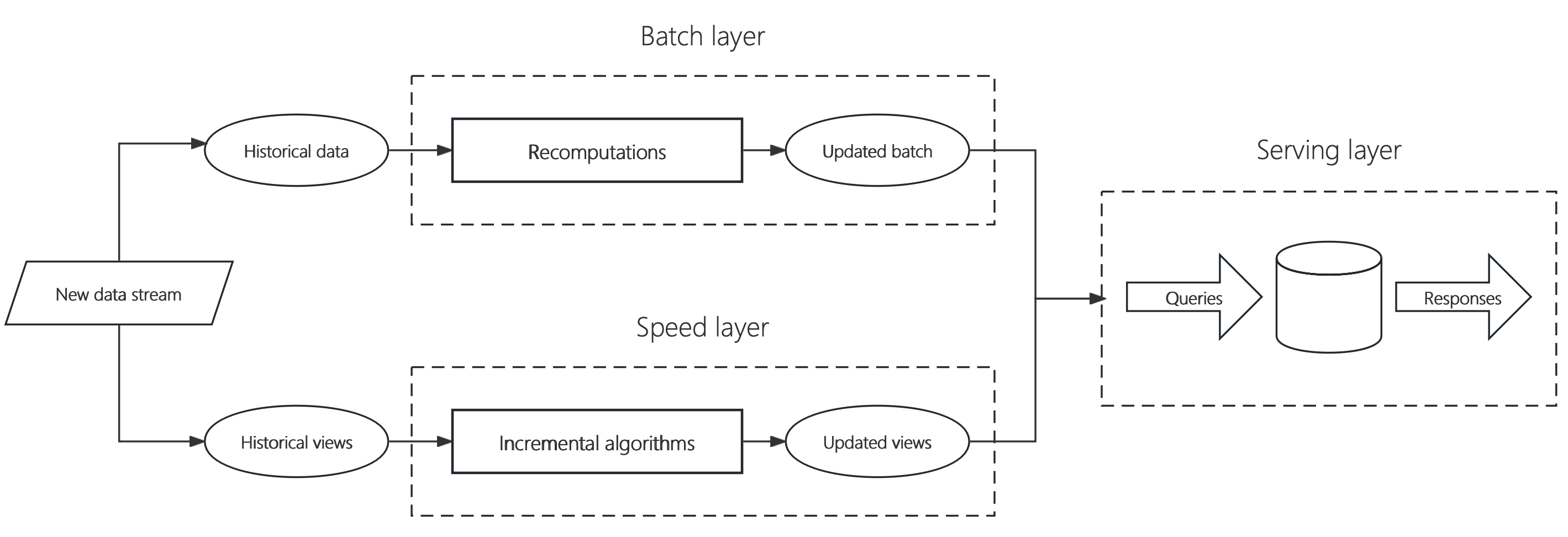
(a) Lambda Architecture

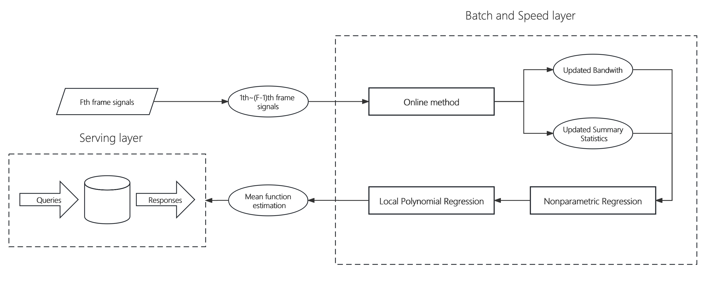
(b) Online Architecture

Figure 1: Lambda architecture concerning new data stream flows. (a) Basic lambda architecture, and (b) online architecture in this paper. The goal of incremental algorithms utilized here is to update previously stored statistics with an incoming batch of data sets.

In traffic monitoring, the demand for efficient communication and data storage is continuously increasing, signal representation and compression are quite important factors [8]. Particularly in the field of optical fiber application, vehicle signals collected by DAS systems are enormous and multi-frame, causing trouble in data redundancy, data asynchronism, processing complexity, memory occupation and real-time requirements [9]. Thus signals need to be preprocessed and compressed according to demands. Traditional signal decompositions such as filter-based Wavelet and Kalman methods, can reconstruct signals from limited observation sets, but are not able to perform data compression. The ineffectiveness of common tools in the field of transportation has led us to explore new ways in the statistical sense.

The signals collected by DAS systems are continuously generated with discretized property and enormous quantities, necessitating real-time processing. It can be viewed as streaming data from the statistical perspective, which refers to a set of data sequences coming in continuously and rapidly, but there is limited memory to store them [10]. Furthermore, signals are recorded at several discrete distance points and have similar properties with functional data, which originates from continuous functions, but due to practical limitations such as technological constraints, are sampled discretely [11]. In terms of definition and properties, multi-frame problems of optical fiber signals can be abstracted into online mean estimation problems of functional data. Moreover, in statistical thought, the trajectory of each subject can be viewed as a stochastic process, while the mean function is modeled nonparametrically with information accumulated to improve the accuracy of estimation [12]. In addition, optical fiber signals have spatial and temporal characteristics, and a series of exploratory methods for spatio-temporal data is applicable in the field of statistics, such as visualization, spectral analysis, Empirical Orthogonal Function (EOF) analysis, Canonical Correlation Analysis (CCA), etc [13]. In the above regard, this paper attempts to employ statistical methods regarding functional data to process optical fiber signals.

Since optical fiber signals are dynamically flowing frame by frame during the acquisition process, signals are required to be processed and analyzed immediately as soon as they enter the system, which is concluded as online processing (also known as real-time processing). With the emerging field of Big Data analytics and real-time applications, numerous online processing methods and technologies have been developed and applied [14]. Among them, statistical online algorithms can better improve the timeliness of information processing, and can also update the database online, which can better connect the database and provide technical support for data preprocessing [15]. Online statistical methods put more emphasis on online processing, performing detection or classification based on information from the past and present, without seeing the future. Based on the non-parametric model and regression method, this research can update bandwidth and summary statistics as signals flow rapidly, boasting three major advantages: (1) It is based on a statistical method and has strong interpretability; (2) it reflects the overall trend and can be updated with a rapid response; and (3) using only summary statistics of previous data, instead of storing entire data is of critical importance in saving computing memory and speed. This online architecture for streaming data analysis can be implemented in the Lambda Architecture design pattern currently used by Twitter and AWS [16]. As illustrated in Fig. 1, (a) shows the standard Lambda Architecture, and (a) shows the specific application in this paper.

This paper is devoted to dealing with multi-frame problems of optical fiber signal preprocessing via statistical methods in real time. An online mean estimation approach based on non-parametric regression is employed [17]. This approach utilizes Local Polynomial Regression (LPR) to estimate the mean value of multi-frame signals, and dynamically update the tuning variable bandwidth in real time under computing memory constraints. This online estimation approach does not have to store all data sets, but storing two summary statistics is sufficient to achieve great accuracy comparable to that of using the entire dataset, which are means of signal compression. The mean estimator is renewed with current streaming data sets and summary statistics of historical data, which is the process of signal reconstruction. Real data examples have demonstrated its effectiveness in many scenarios, such as airline delay prediction and online news data estimation. The work of this paper is to apply this online algorithm in the realm of Intelligent Transportation Systems, enabling the estimation of mean functions based on historical summary statistics in conjunction with current data. Additionally, we go further to extract fiber stripes from waterfall diagrams to validate the impact of the algorithm on subsequent vehicle trajectory extraction algorithms. The statistical method used in this paper is compared with filter-based methods, considering 1-D signal amplitudes and 2-D waterfall diagram information, showing its effectiveness in practical highway scenarios.

The main contributions of this paper are as follows:

1. We abstract signal processing problems in DAS systems as a non-parametric regression problem in the field of statistics.

2. We use the Local Polynomial Regression method to extract summary statistics for signal compression. As signals flow in frame by frame, we can also update the estimator and perform signal reconstruction with rapid responses in real time.

3. Our proposed technique provides a basis for the preprocessing of signals and can be further applied to Intelligent Transportation Systems.

The remainder of this paper is as follows. Section II introduces DAS technology, local polynomial regression and online lambda architecture. Section III displays the methodology, including online mean estimation method and trajectory extraction algorithm. Section IV introduces the design of experiments and discusses the experimental result. Section V provides conclusions and limitations of this study.

II Related Works

II-A Distributed Acoustic Sensing Technology

Distributed Acoustic Sensing (DAS) is a rapidly developed passive fiber-optic sensing technology, which can detect acoustic signals anywhere along the length of fiber with high-frequency responses and tight spatial resolution [18]. DAS not only has the advantages of traditional fiber-optic sensing technologies (e.g., anti-electromagnetic interference, corrosion resistance, slenderness, and flexibility) but can also measure dynamic strains like vibrations and sound waves along fiber paths in a long-distance, fully distributed, and online manner. Given the considerable application values of DAS, a growing number of experts and scholars are exploring its possibility in Intelligent Transportation Systems (ITS). They are exploring its potential for vehicle traffic monitoring, making traffic detection methods based on the DAS system a focal point of recent research and development. Detection of vehicle speed, density, and road conditions can be achieved using fiber-carrying high-speed data transmission [19].

Generally speaking, the Optical Fiber System, highlighted by its DAS technology, boasts three major advantages. Firstly, its all-weather capability ensures effective operation under a variety of adverse weather conditions such as rain, snow, fog, and wind, maintaining functionality both during the day and night. Secondly, the system offers comprehensive tracking by enabling online monitoring of all vehicles over extensive road sections, thereby eliminating the necessity for integration with multiple poles or sensors. Lastly, it showcases green and cost-efficiency as a single fiber strand can span up to 40 kilometers, significantly cutting down on construction and maintenance costs while exemplifying green energy efficiency.

II-B Local Polynomial Regression

Local Polynomial Regression (LPR) is a non-parametric technique for smoothing scatter plots and modeling functions [20], which combines the advantages of Polynomial Regression and Linear Weighted Regression. LPR uses the information of neighboring sample points to estimate current data points through local weighting, and has great regression performance for nonlinear models.

Suppose that $\{(x_{i},y_{i})|x_{i}\in\mathbb{R}^{n},y_{i}\in\mathbb{R}^{n}\}_{i=1}^{n}$ are random samples from the non-parametric regresssion model:

$$y_{i}=f(x_{i})+\epsilon_{i}$$ (1)

where $y_{i}$ is the response variable, $x_{i}$ is the explanatory variable, $f(\cdot)$ is a non-parametric smoothing function, and $\epsilon_{1},...,\epsilon_{n}$ are uncorrelated random errors with mean 0 and variance $\sigma^{2}$. Now we need to solve $E(y_{i}|x_{i})=f(x_{i})$ for its best estimation $\widehat{f}(x_{i})$.

The main idea of LPR is to estimate $f(\tilde{x})$ using points $x$ adjacent to the current point $\tilde{x}$. Using the Taylor expansion, Taylor series for $f(x)$ at point $\tilde{x}$ is:

$$f(x;\tilde{x})=f(\tilde{x})+\sum_{j=1}^{\infty}\frac{f^{(j)}(\tilde{x})}{j!}(x-\tilde{x})^{j}$$ (2)

Take the first $p+1$ terms of the series and denote $\beta_{0}=f(\tilde{x}),\beta_{j}=\frac{f^{(j)}(\tilde{x})}{j!}$, the above formula can be simplified as:

$$f_{p}(x;\tilde{x})=\beta_{0}+\sum_{j=1}^{p}\beta_{j}(x-\tilde{x})^{j}$$ (3)

where $p$ is the order of polynomial fit.

LPR introduces the concept of weights and utilizes a low-order weighted least squares (WLS) regression to fit. The weight $\omega$ is usually measured by kernel function $K_{h}(\cdot)$, which depends on bandwidth $h$. Bandwidth measures the complexity of LPR. The larger the bandwidth is, the more sample points will be used to estimate $\widehat{y}$, and the weight assigned to each sample point will be smaller. The weight gap between near sample points and far sample points is not so large, and the fitting curve will be smoother. However, due to the use of a large number of sample point information with no local property, the deviation of estimation will be relatively larger. And vice versa. Therefore, an optimal bandwidth must achieve a balance between empirical error and generalization error.

Based on the above, denote the weight $\omega_{i}$ is the weight between $\tilde{x}$ and its neighbor point $x_{i}$, and a one-dimensional kernel function is used for LPR, then the weight can be expressed as:

$$\omega_{i}=K_{h}(x_{i};\tilde{x})=\frac{1}{h}K(\frac{x_{i}-\tilde{x}}{h})$$ (4)

The least squares estimate of the model is usually obtained by minimizing the weighted Residual Sum of Squares (RSS). Through multiplying the weight function $\omega_{i}$ and the loss $(y_{i}-f_{p}(x_{i};\tilde{x}))^{2}$ at each point around $\tilde{x}$, RSS of LPR can be written as:

$$RSS(\beta)=\sum_{i=1}^{n}(y_{i}-f_{p}(x_{i};\tilde{x}))^{2}\omega_{i}=(y-\Phi\beta)^{T}\Omega(y-\Phi\beta)$$ (5)

where $\Omega={\rm{diag}}(\omega_{1},\omega_{2},...,\omega_{n}),y=(y_{1},y_{2},...,y_{n})^{T},\beta=(\beta_{0},\beta_{1},...,\beta_{p})^{T}$,

$$\Phi=\begin{pmatrix}1&x_{1}-\tilde{x}&(x_{1}-\tilde{x})^{2}&\cdots&(x_{1}-\tilde{x})^{p}\\ 1&x_{2}-\tilde{x}&(x_{2}-\tilde{x})^{2}&\cdots&(x_{2}-\tilde{x})^{p}\\ \vdots&\vdots&\vdots&\ddots&\vdots\\ 1&x_{n}-\tilde{x}&(x_{n}-\tilde{x})^{2}&\cdots&(x_{n}-\tilde{x})^{p}\end{pmatrix}$$ (6)

Take the partial derivative of $\beta$ to minimize the loss function, and we get the estimate of $\beta$:

$$\widehat{\beta}=(\Phi^{T}\Omega\Phi)^{-1}\Phi^{T}\Omega y$$ (7)

Plug the above estimates into the formula (3) and the mean estimation for each sample point is:

$$\widehat{y}_{i}=\widehat{f}(x_{i};\tilde{x})=\widehat{\beta}_{0}+\sum_{j=1}^{p}\widehat{\beta}_{j}(x_{i}-\tilde{x})^{j}$$ (8)

As can be seen from the above, LPR is a kernel-based estimator, which has the form of locally weighted least squares. According to the theoretical results of optimal variable bandwidths, which would be the ideal bandwidth to work with, $h\propto\frac{1}{n}$ [21]. Therefore, the bandwidth should be indicated by the streaming data themselves, and be updated by a data-driven bandwidth selection procedure.

II-C Lambda Architecture

Lambda architecture is a Big Data system of computing and storage with synchronized processing of batch and stream data flows, consisting of three layers [22]:

1. Batch layer continuously recomputes previously-stored batch views when a new batch of data arrives, achieving data accuracy by processing all existing historical data.

2. Speed layer utilizes incremental algorithms to update old online views with an incoming batch of data, minimizing latency by providing a real-time view of the newest data.

3. Serving layer stores the view outputs of the above two layers and responds to queries.

Not only the data integrity is taken into account through the batch layer, but also the high delay of batch layer can be compensated by speed layer, making the whole query real-time. The basic lambda architecture of how it works is illustrated in Fig. 1 (1). The lambda architecture enables us to facilitate sequential updating of summary statistics used in estimation, and is flexible and scalability to a wide range of streaming data analyses in which the batch layer stores all accumulated data and produces reliable results. Moreover, it enables developers to build large-scale distributed data processing systems and is tolerant of hardware failure and human error.

III Method

III-A Problem Formulation

In the acquisition process of the Distributed Acoustic Sensor (DAS) system, the length of optical fiber is fixed and we denote sampling points as $d\in\{1,2,...,D\}$. Denote the acquisition Frames Per Second (FPS) in optical fiber systems by $F_{\rm max}$ and the max number of seconds collected by $S$. Then signal amplitude at each frame-distance vector can be expressed as $A^{s}_{f}=(a^{s}_{f1},a^{s}_{f2},...,a^{s}_{fD}),f\in\{1,2,...,F_{\rm max}\},s\in\{1,2,...,S\}$, where $a^{s}_{fd}\in\mathbb{R^{+}}$ is signal amplitude. If the data matrix collected at second $s$ is denoted as $A^{s}$, it can be expressed as:

$$A^{s}=\begin{pmatrix}A^{s}_{1}\\ A^{s}_{2}\\ \vdots\\ A^{s}_{F_{\rm max}}\end{pmatrix}=\begin{pmatrix}a^{s}_{11}&a^{s}_{12}&\cdots&a^{s}_{1D}\\ a^{s}_{21}&a^{s}_{22}&\cdots&a^{s}_{2D}\\ \vdots&\vdots&\ddots&\vdots\\ a^{s}_{F_{\rm max}1}&a^{s}_{F_{\rm max}2}&\cdots&a^{s}_{F_{\rm max}D}\end{pmatrix}$$ (9)

It should be noted that the flow of signals can be regarded as streaming data over time, and if the total signals are accumulated to the second $S$, the complete matrix can be represented as $A=(A^{1},A^{2},...,A^{S})^{T}$. Due to FPS setting of the DAS system, the fiber signals are multi-frame recorded and we need to export the specific number of frames according to the requirements.

Although signals are collected at discrete points, we can reduce them to 1-D continuous information for further modeling analysis. In addition, we generalize the above questions to take into account the possibility of changing the location of the collection point, which is, that the distance point and observations may vary due to artificial setup. The 1-D amplitude information $\{A_{f}(X_{fd}):X_{fd}\in\mathcal{X}\}$ can be considered as an $L^{2}$ stochastic process on a distance interval $\mathcal{X}$ for each frame $f\in\{1,...,F_{\rm max}\}$. In each frame $f$, we have a subject with $D$ observations at discrete distance point $X_{fd},d\in\{1,...,D\}$, so observations can be written in discrete form:

$$A_{f}(X_{fd})=\mu(X_{fd})+\Phi_{f}(X_{fd})$$ (10)

where $\mu(\cdot)$ is mean function, $\Phi(\cdot)$ is stochastic part. Attention that our observations are contaminated with noises in practical application. To describe the stochastic process more accurately, we introduce white noise and rewrite the observations:

$$Y_{fd}=A_{f}(X_{fd})+\epsilon_{fd}=\mu(X_{fd})+\Phi_{f}(X_{fd})+\epsilon_{fd}$$ (11)

where $\epsilon_{fd}$ are independently and identically distributed(i.i.d) noises with $E(\epsilon_{fd})=0$ and ${\rm Var}(\epsilon_{fd})=\sigma^{2}$.

FPS in optical fiber systems is set manually, where a higher sampling rate implies more data points to be collected and more signal details to be captured. However, when signals are output as structured data in practical applications, it is not necessary to use all multiple frames of data, and storing them consumes significant memory. Therefore, how to handle high frame rate signals in fiber-based optic systems poses a challenge. Moreover, distinguishing the trajectory of each vehicle and conducting traffic flow statistics is also a great challenge. How to deal with multi-frame signals in each frame and extract trajectories accurately is the primary objective of this paper.

III-B Online Mean Estimation

Based on the above analysis of optical fiber signals and the non-parametric model, the Local Polynomial Regression (LPR) method is adopted to estimate the mean function. In our experiments, the common Epanechnikov kernel function for non-parametric filtering and data smoothing is employed as kernel function $K(\cdot)$ in (4), and the formula is as follows:

$$K(x)=\begin{cases}\frac{3}{4}(1-x^{2}),&|x|<1;\\ 0,&|x|\geq 1.\end{cases}$$ (12)

Since optical fiber signals can be seen as streaming data flowing in continuously, and bandwidth is inversely proportional to the amount of data [21]. The online mean estimation algorithm pays particular attention to bandwidth selection. Future optimal bandwidth is approximated by a corresponding online estimator, and a dynamic candidate bandwidth sequence is utilized to select the most suitable one. After that, historical summary statistics are combined to form the updated summary statistics and mean function estimations.

For notations, the subscript $\widehat{}$ and $\widetilde{}$ denote the classical batch method using full data and the online method using only the $f$th data and stored summary statistics respectively.

III-B1 Classical Batch Method

Based on the non-parametric modeling of optical fiber signals in (11), we can use the Local Polynomial Regression model in Section II-B to derive mean function estimation. For the sake of simplicity, a first-order LPR model ($p=1$) is used, the simple regression model is:

$$Y_{fd}=\beta_{0}+\beta_{1}X_{fd}+\epsilon_{fd}$$ (13)

By minimizing the loss function based on the weighted Residual Sum of Squares (RSS), we get the estimation of $(\beta_{0},\beta_{1})$:

$$\begin{split}(\widehat{\beta}_{0},\widehat{\beta}_{1})=\arg\min\limits_{\beta_{0},\beta_{1}}\sum_{f=1}^{F}\sum_{d=1}^{D}\left\{Y_{fd}-\beta_{0}-\beta_{1}(X_{fd}-x)\right\}^{2}\\ \times K_{\widehat{h}^{(F)}}(X_{fd}-x)\end{split}$$ (14)

where $\widehat{h}_{\mu}^{(F)}$ is the bandwidth using the full data up to $F(F\leq F_{\rm max})$. Let $e_{2}=(1,0)^{T}$, $X_{fd}(x)=(1,X_{fd}-x)^{T}$, and the solution of classical mean estimation at block $F$: $\widehat{\mu}^{(F)}(x)=\widehat{\beta}_{0}$ can be explicitly rewritten as:

$$\widehat{\mu}^{(F)}(x)=e_{2}^{T}\left\{\sum_{f=1}^{F}P_{f}(x;\widehat{h}^{(F)}_{\mu})\right\}^{-1}\left\{\sum_{f=1}^{F}Q_{f}(x;\widehat{h}^{(F)}_{\mu})\right\}$$ (15)

where $\{P_{f},Q_{f}\}$ only depends on the $f$th frame given bandwidth $\widehat{h}_{\mu}^{(F)}$ by

$$P_{f}(x;\widehat{h}^{(F)}_{\mu})=\sum_{d=1}^{D}K_{\widehat{h}^{(F)}_{\mu}}(X_{fd}-x)X_{fd}(x)X_{fd}(x)^{T}$$ (16)

$$Q_{f}(x;\widehat{h}^{(F)}_{\mu})=\sum_{d=1}^{D}K_{\widehat{h}^{(F)}_{\mu}}(X_{fd}-x)X_{fd}(x)Y_{fd}$$ (17)

From the formulations above, such kernel-based mean estimator can be decomposed into two summary statistics $\sum_{f=1}^{F}P_{f}(x;\widehat{h}^{(F)}_{\mu})$ and $\sum_{f=1}^{F}Q_{f}(x;\widehat{h}^{(F)}_{\mu})$, which are additive on data depending on the tuning variable bandwidth $\widehat{h}^{(F)}_{\mu}$. Given the bandwidth, we only need to store a pair of precise summary statistics in computing memory instead of the entire $F$ data frames, which is highlighted in the era of Big Data.

III-B2 Online Estimation

According to the theoretical result of LPR, bandwidth is inversely proportional to the sample size. As frame $F$ varies, the sample size of signals gradually varies, bandwidth of classical batch method $\widehat{h}^{(F)}_{\mu}$ may take different values. As the number of frames increases to the maximum $F_{\rm max}$, this data-driven feature has to store all summary statistics $\left\{\sum_{f=1}^{F}P_{f}(x;\widehat{h}^{(F)}_{\mu}),\sum_{f=1}^{F}Q_{f}(x;\widehat{h}^{(F)}_{\mu})\right\}_{F=1}^{F_{\rm max}}$. To overcome this obstacle and respond to streaming data in real time, a method to update statistics based on dynamic candidate bandwidth sequence is adopted.

Denote $h_{\mu,*}^{(f)}$ as the optimal bandwidth of the $f$th frame for $f\leq F_{\rm max}$ and $\widetilde{h}^{(f)}_{\mu}$ as its corresponding online estimator. The expression of both are shown in [17, Section 4]. According to [17, Theorem 3], the online bandwidth estimator $\widetilde{h}^{(f)}_{\mu}$ satisfies that as $f\rightarrow\infty$:

$$\frac{\widetilde{h}^{(f)}_{\mu}-h_{\mu,*}^{(f)}}{h_{\mu,*}^{(f)}}=O_{p}(f^{-\frac{1}{5}})$$ (18)

where $O_{p}$ means bounded in probability [23]. The formula above implies the online estimator $\widetilde{h}^{(F)}_{\mu}$ converges to the optimal bandwidth $h_{\mu,*}^{(F)}$, and can serve as a surrogate of it.

According to the characteristics of streaming data and the inverse relationship between bandwidth and sample size, if the whole data is not used for calculation when new data flows in, we need to update the previous bandwidth. Following the strategies in [17], the calculation of the $F$th frame signals mean estimation is by recursion as follows.

Let $\{\eta_{\mu,l}^{(f)}\}_{l=1}^{L}$ for $f<F$ be the dynamic candidate bandwidth sequence with

$$\eta_{\mu,l}^{(f)}=(\frac{L-l+1}{L})^{\frac{1}{5}}\widetilde{h}_{\mu}^{(f)}$$ (19)

and let $\{\phi_{\mu,l}^{(f-1)}\}_{l=1}^{L}$ be the centroids (i.e.weighted average of all previous candidate bandwidths):

$$\phi_{\mu,l}^{0}=0,\phi_{\mu,l}^{(f)}=(1-\frac{1}{f})\phi_{\mu,j_{l}^{(f)}}^{(f-1)}+\frac{1}{f}\eta_{\mu,l}^{(f)},$$ (20)

where

$$j_{l}^{(f)}=\arg\min\limits_{i\in\{1,2,...,L\}}\left|\eta_{\mu,l}^{(f)}-\phi_{\mu,i}^{(f-1)}\right|.$$ (21)

The choice of $j_{l}^{(f)}$ in the formula guarantees that $\phi_{\mu,j_{l}^{(f)}}^{(f-1)}$ is close to $\eta_{\mu,l}^{(f)}$, which makes $\phi_{\mu,l}^{(f)}$ close to $\eta_{\mu,l}^{(f)}$ as well. As a result, we get the most suitable bandwidth $\eta_{\mu,j_{l}^{(f)}}^{(f)}$ and output the $f$th summary statistics whenever needed.

To combine information across frames, the so-called “pseudo-summary statistics” $\{\widetilde{P}_{\mu,l}^{(f)},\widetilde{Q}_{\mu,l}^{(f)}\}_{l=1}^{L}$, whose update depends only on the sub-statistics of the current frame $\{P_{f},Q_{f}\}$ which are calculated following formulas (16) and (17), and the stored pseudo-summary statistics of previous frames $\{\widetilde{P}^{(f-1)}_{\mu,j_{l}^{(f)}},\widetilde{Q}^{(f-1)}_{\mu,j_{l}^{(f)}}\}$. the pseudo-summary statistics can be expressed as:

$$\widetilde{P}_{\mu,l}^{(f)}(x)=P_{f}(x;\eta_{\mu,l}^{(f)})+\widetilde{P}^{(f-1)}_{\mu,j_{l}^{(f)}}(x)$$ (22)

$$\widetilde{Q}_{\mu,l}^{(f)}(x)=Q_{f}(x;\eta_{\mu,l}^{(f)})+\widetilde{Q}^{(f-1)}_{\mu,j_{l}^{(f)}}(x)$$ (23)

with initialization $\widetilde{P}_{\mu,l}^{(0)}(x)=0,\widetilde{Q}_{\mu,l}^{(0)}(x)=0$ for $l\in\{1,2,...,L\}$.

It’s worth noting that $\{\eta_{\mu,l}^{(f)}\}_{l=1}^{L}$ and $\{j_{l}^{(f)}\}_{l=1}^{L}$ are recalculated at each $f$, and only the newest $\{\phi_{\mu,l}^{(f)}\}_{l=1}^{L}$ and $\{\widetilde{P}_{\mu,l}^{(f)},\widetilde{Q}_{\mu,l}^{(f)}\}_{l=1}^{L}$ are stored in memory during the procedure. Hence the algorithm is computationally efficient.

Follow the recursive process above and note that $\eta_{\mu,1}^{(F)}=\widetilde{h}^{(F)}_{\mu}$ in formula (19), the mean estimation at frame $F$ is given by:

$$\widetilde{\mu}^{(F)}(x)=e_{2}^{T}\left\{\widetilde{P}_{\mu,1}^{(F)}(x)\right\}^{-1}\left\{\widetilde{Q}_{\mu,1}^{(F)}(x)\right\}$$ (24)

Hence the online mean estimation of multi-frame signals are effectively achieved.

III-C Trajectory Extraction

During the trajectory extraction processing of optical fiber signals, we represent them as three-dimensional waterfall diagrams. Based on these diagrams, we utilize a vehicle position detection algorithm and a vehicle trajectory extraction algorithm to achieve detection and overall tracking for vehicles.

After the preprocessing of optical fiber signals, we use the first column information, which is processed by Butterworth Filter and peaks location search method, to determine the vehicles’ entry times. Then, an algorithm for line-by-line matching based on the vehicle motion model to track key points of vehicle trajectories. Then we can reconstruct the complete vehicle trajectories and subsequently calculate the instantaneous speed of the vehicles.

IV Experiments

IV-A Datasets

Experiments are implemented on real highway scenarios for data acquisition and data analysis. Jingjintang Expressway (Junliang City Test Site, Dongli District, Tianjin, China) is a real highway scenario of a dual carriageway with three lanes in each direction. We selected 320 meters section of Jingjintang Expressway. The aerial view of this highway is illustrated in Fig. 2.

Our DAS system collected vibration signals of vehicles at a rate of 3 frames per second, with each point at 0.4 meters, for a total duration of 2 hours and 5 minutes, which is equivalent to 7500 seconds. The total length of the optical fiber acquisition distance is 320 meters, corresponding to 800 distance points. When the vehicle traverses the area, the DAS system will record the corresponding vibration signals. We present the vibration signals recorded by the DAS system during the passage of a single truck and a single car through the target area as shown in Fig. 3.

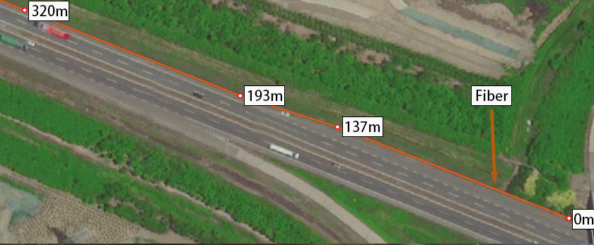
Figure 2: Overhead view of the Jingjintang expressway, and the optical fiber is laid on one side of the road.

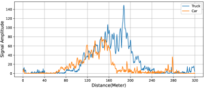
Figure 3: A single vehicle passes through the highway where the optical fiber is laid.

As can be seen from the two types of vehicle driving signals above, their amplitude and duration are quite different. To show the vehicles’ trajectory more intuitively, we employ waterfall diagrams to plot the collected signal values, as shown in Fig. 4.

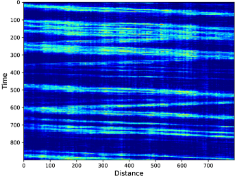
Figure 4: The raw optical fiber waterfall diagram in part of highway scenarios.

In waterfall diagrams, the light blue color represents background noise, whereas the prominently colored lines represent vehicles. The fiber stripes extending from the top left to the bottom right represent vehicles within the target area, while the stripe extending from the top right to the bottom left represents vehicles on the opposite side. Furthermore, the vehicle’s trajectory is depicted as an approximately straight line within the diagram, as most vehicles on the highway maintain high and consistent velocities when traveling in lanes with unchanged speed. The intercept of the straight line represents the starting position of the vehicle, and the absolute value of the slope represents its velocity.

IV-B Quantitative analysis

The algorithm performance is validated on real highway scenarios, which are located in Junliang City Test Site, Dongli District, Tianjin, China. In particular, a vehicle trajectory extraction algorithm is adopted to analyze the processed optical fiber signals. We also compared with the Wavelet Filter and Kalman Filter to verify the effectiveness of the proposed online mean estimation algorithm.

We randomly selected two seconds of signals for presentation with each second corresponding to three frames, as illustrated in Fig. 5. The blue lines represent online mean estimation results for three frames of colored lines. It can be seen that the online mean estimation method can effectively show the trends of multi-frame signals, especially for estimating the peak position of multi-frame data.

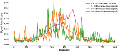
(a) $s=1$

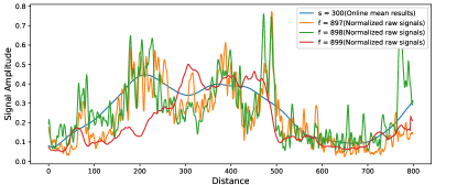
(b) $s=300$

Figure 5: The mean estimation curve of multiple-frame signals compared with normalized raw signals, where $s$ represents the processed seconds and $f$ represents the frame in raw signals.

Furthermore, we carried out comparative experiments with the filter-based Kalman and Wavelet Filter, employing the same preprocessing steps. Wavelet filtering is a signal processing method based on time-frequency analysis, which can decompose and reconstruct signals at different resolutions. Kalman filtering is a recursive and optimal linear filtering algorithm. Based on Bayesian filtering theory, the Kalman filter is used to estimate the state variables of the system by using the dynamics model and the observation model of the system. Since the filtering process of the two methods cannot directly average the multi-frame signals, the method adopted in this paper is to filter the multi-frame data first and then take the average value for comparison and analysis with online mean estimation.

In real applications, optical fiber signals collected by the DAS system are discretely related to time and distance. Frames Per Second (FPS) are only related to time. On one hand, to process multi-frame data, we present signals as distance-dependent one-dimensional line graphs. On the other hand, to display traffic flow more intuitively, we present signals as three-dimensional waterfall diagrams for vehicle detection algorithms. Here we take two contrasting approaches, considering 1-D signal amplitudes and 2-D waterfall diagram information.

In 1-D signal amplitudes analysis, considering the subsequent vehicle trajectory extraction algorithm, we need to determine the vehicle entry situation through the peaks of the starting position. Therefore, we compared the signal processing results of the above algorithm for the first column. As depicted in Fig. 6, mean estimation method and the two Filters have excellent noise attenuation effects on the raw signals, and the burr phenomenon of the raw signals is obviously reduced. It is worth mentioning that the algorithm in this paper can amplify the original large truck signals, while the small car signals maintain the original small value, and the bottom noise is also maintained in a relatively stable small base range, so our algorithm shows superior accuracy in extracting vehicle trajectories.

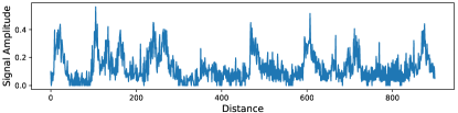
(a) Raw

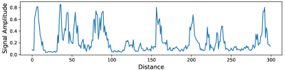
(b) Online

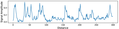
(c) Kalman

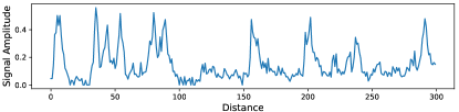
(d) Wavelet

Figure 6: Comparation of 1-D processed signals. (a) Normalized raw signals, (b) Online mean estimation, (c) Kalman Filter, and (d) Wavelet Filter.

In 2-D waterfall diagram information, we can see direct comparisons of different algorithms, as shown in Fig. 7. In the fiber waterfall diagrams, the prominently colored lines represent vehicle signals extracted by DAS, and the light blue color represents the background noise. Compared with the other methods, our method attains smoother diagrams, with obvious background noise removal effects and stronger signals for the vehicles.

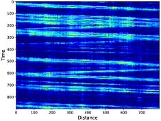
(a) Raw

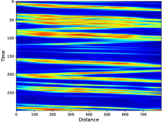
(b) Online

(c) Kalman

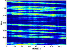
(d) Wavelet

Figure 7: The mean estimation waterfall diagrams of multiple-frame signals compared with normalized raw signals, Kalman Filter, and Wavelet Filter.

Based on preprocessed multi-frame signals, we also utilize a vehicle trajectory extraction algorithm with the same parameters to examine the effectiveness of subsequent structured data extraction. As displayed in Fig. 8, compared to normalized raw signals, the online estimation method and the two filter-based methods are all able to extract trajectories consistent with fiber stripes. In particular, the online mean estimation algorithm is more precise in extracting finer fiber stripes.

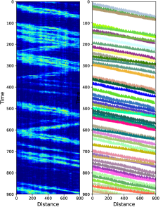
(a) Raw

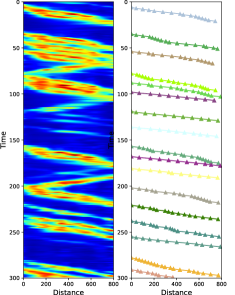
(b) Online

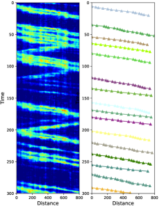
(c) Kalman

(d) Wavelet

Figure 8: The vehicle trajectory extraction results of multiple-frame signals compared with normalized raw signals, Kalman Filter, and Wavelet Filter.

V Conclusion

In this paper, we have demonstrated the application of optical fiber-based Distributed Acoustic Sensors (DAS) systems to monitor traffic flow in real highway scenarios. An online mean estimation method is utilized to deal with multi-frame problems in signal preprocessing. Compared with existing filter-based methods, such as Kalman Filter and Wavelet Filter, the online method achieves real-time processing while saving computing memory, demonstrating its superiority. The major conclusions and areas for improvement in this research are as follows:

(1) The problem of multi-frame signals is characterized by a non-parametric regression model, and the mean function is fitted by a Local Polynomial Regression rather than averaging directly, which cannot be solved by filter-based methods.

(2) The online method using only summary statistics of previous data, instead of historical raw data, is of critical importance in handling big data as far as computing memory and speed are concerned.

(3) In this paper, signals are stored as summary statistics and applied to mean estimation problems. In addition, other applications of statistics in the field of transportation can be explored, such as spatio-temporal prediction, outlier detection, etc.

Declaration of Competing Interest

The authors declare that they have no known competing financial interests or personal relationships that could have appeared to influence the work reported in this paper.

References

- [1] T. M. Daley, B. M. Freifeld, J. Ajo-Franklin, S. Dou, R. Pevzner, V. Shulakova, S. Kashikar, D. E. Miller, J. Goetz, J. Henninges, et al., “Field testing of fiber-optic distributed acoustic sensing (das) for subsurface seismic monitoring,” The Leading Edge, vol. 32, no. 6, pp. 699–706, 2013.
- [2] M. Litzenberger, C. Coronel, K. Bajic, C. Wiesmeyr, H. Döller, H.-B. Schweiger, and G. Calbris, “Seamless distributed traffic monitoring by distributed acoustic sensing (das) using existing fiber optic cable infrastructure,” REAL CORP, 2021.
- [3] Y. Wang, H. Yuan, X. Liu, Q. Bai, H. Zhang, Y. Gao, and B. Jin, “A comprehensive study of optical fiber acoustic sensing,” IEEE access, vol. 7, pp. 85821–85837, 2019.
- [4] H. Liu, J. Ma, W. Yan, W. Liu, X. Zhang, and C. Li, “Traffic flow detection using distributed fiber optic acoustic sensing,” IEEE Access, vol. 6, pp. 68968–68980, 2018.
- [5] H. Liu, J. Ma, T. Xu, W. Yan, L. Ma, and X. Zhang, “Vehicle detection and classification using distributed fiber optic acoustic sensing,” IEEE Transactions on Vehicular Technology, vol. 69, no. 2, pp. 1363–1374, 2019.
- [6] M. Wang, Z. Li, J. Zhang, and Y. Zhong, “Vehicle trajectory extraction based on distributed fiber sensing system,” Engineering Science and Technology, vol. 53, no. 2, pp. 141–150, 2021.
- [7] C. Wiesmeyr, C. Coronel, M. Litzenberger, H. J. Döller, H.-B. Schweiger, and G. Calbris, “Distributed acoustic sensing for vehicle speed and traffic flow estimation,” in 2021 IEEE international intelligent transportation systems conference (ITSC), pp. 2596–2601, IEEE, 2021.
- [8] K. Engan, “Frame based signal representation and compression,” 2000.
- [9] J. Pokornỳ, P. Škoda, I. Zelinka, D. Bednárek, F. Zavoral, M. Kruliš, and P. Šaloun, “Big data movement: a challenge in data processing,” Big Data in Complex Systems: Challenges and Opportunities, pp. 29–69, 2015.
- [10] S. Muthukrishnan et al., “Data streams: Algorithms and applications,” Foundations and Trends® in Theoretical Computer Science, vol. 1, no. 2, pp. 117–236, 2005.
- [11] J.-L. Wang, J.-M. Chiou, and H.-G. Müller, “Functional data analysis,” Annual Review of Statistics and its application, vol. 3, pp. 257–295, 2016.
- [12] F. Ferraty, Nonparametric functional data analysis. Springer, 2006.
- [13] N. Cressie and C. K. Wikle, Statistics for spatio-temporal data. John Wiley & Sons, 2015.
- [14] T. Zheng, G. Chen, X. Wang, C. Chen, X. Wang, and S. Luo, “Real-time intelligent big data processing: technology, platform, and applications,” Science China Information Sciences, vol. 62, pp. 1–12, 2019.
- [15] C. Hammer, M. D. C. Kostroch, and M. G. Quiros, Big data: Potential, challenges and statistical implications. International Monetary Fund, 2017.
- [16] J. Warren and N. Marz, Big Data: Principles and best practices of scalable realtime data systems. Simon and Schuster, 2015.
- [17] Y. Y. Fang Yao, “Online estimation for functional data,” Journal of the American Statistical Association, pp. 1–15, 2021.
- [18] R. Cannon and F. Aminzadeh, “Distributed acoustic sensing: State of the art,” in SPE Digital Energy Conference and Exhibition, pp. SPE–163688, SPE, 2013.
- [19] G. A. Wellbrock, T. J. Xia, M.-F. Huang, Y. Chen, M. Salemi, Y.-K. Huang, P. Ji, E. Ip, and T. Wang, “First field trial of sensing vehicle speed, density, and road conditions by using fiber carrying high speed data,” in 2019 Optical Fiber Communications Conference and Exhibition (OFC), pp. 1–3, IEEE, 2019.
- [20] M. Avery, “Literature review for local polynomial regression,” Unpublished manuscript, 2013.
- [21] J. Fan and I. Gijbels, “Data-driven bandwidth selection in local polynomial fitting: variable bandwidth and spatial adaptation,” Journal of the Royal Statistical Society: Series B (Methodological), vol. 57, no. 2, pp. 371–394, 1995.
- [22] L. Luo and P. X.-K. Song, “Renewable estimation and incremental inference in generalized linear models with streaming data sets,” Journal of the Royal Statistical Society Series B: Statistical Methodology, vol. 82, no. 1, pp. 69–97, 2020.
- [23] V. AWvd, “Asymptotic statistics. cambridge series in statistical and probabilistic mathematics,” 1998.