Fabrication uncertainty aware and robust design optimization of a photonic crystal nanobeam cavity by using Gaussian processes

Abstract

We present a fabrication uncertainty aware and robust design optimization approach that can be used to obtain robust design estimates for nonlinear, nonconvex, and expensive model functions. It is founded on Gaussian processes and a Monte Carlo sampling procedure, and assumes knowledge about the uncertainties associated with a manufacturing process. The approach itself is iterative. First, a large parameter domain is sampled in a coarse fashion. This coarse sampling is used primarily to determine smaller candidate regions to investigate in a second, more refined sampling pass. This finer step is used to obtain an estimate of the expected performance of the found design parameter under the assumed manufacturing uncertainties. We apply the presented approach to the robust optimization of the Purcell enhancement of a photonic crystal nanobeam cavity. We obtain a predicted robust Purcell enhancement of $\overline{F}_{\mathrm{P}}\approx 3.3$. For comparison we also perform an optimization without robustness. We find that an unrobust optimum of $F_{\mathrm{P}}\approx 256.5$ dwindles to only $\overline{F}_{\mathrm{P}}\approx 0.7$ when fabrication uncertainties are taken into account. We thus demonstrate that the presented approach is able to find designs of significantly higher performance than those obtained with conventional optimization.

1 Introduction

The development of new nanophotonic devices is a challenging task that is fueled especially by advances in computing power and powerful algorithms – both, for optimizations [1, 2, 3, 4, 5] and for solving Maxwell’s equations [6, 7, 8]. Nowadays, many innovations in the field stem from inverse design approaches [9, 4]. Here, parameterized computer models, typically numerically discretized models of the envisioned devices are created, e.g., by using the finite element method, and the parameters of these models are varied systematically such that a design is identified that results in a device with optimal figures of merit. This simulation and optimization approach allows to explore a large number of possible device configurations and is much more economical than pure laboratory development.

The modeled nanophotonic devices coming out of these processes often have optimized figures of merit, e.g., maximized quality factor of an optical resonator, with record breaking performance values [10]. When it is time for the manufacturing step of the device, however, the performance values are usually not realized to the predicted extent. This happens even in the cases where the computer model faithfully captures the physical reality and where numerical discretization errors are controlled to sufficiently low levels. Instead, the reason for the deviation is frequently cited as lacking control over the process windows of the manufacturing method [11, 12, 13]. A possible explanation for this is that the very good theoretical results found using the computer model are due to, e.g., fragile resonance effects [14] where the results are part of a narrow ridge in the parameter space, that vanish if some of the model parameters are varied only slightly.

In some instances, to deal with the issue, researchers have employed a mass production approach in which a large number of devices were manufactured and subsequently quantified – a step after which only viable samples were retained [15]. This approach leaves much to be desired in an industrial context, where it is favorable to go from computer model to physical device and have consistent and coherent results at each design step. Rejecting a large number of samples is simply not economical. This requirement adds a new layer of complexity to the design process.

Finding optima that preserve their quality in the face of model parameter uncertainties is the task of robust optimization [16, 17]. Here, a large focus is placed on convex and linear problems [18, 19, 20], in which one often attempts to optimize for the worst case. However, linear convex optimization methods are typically not useful for the robust optimization of computer model based designs, since these models can generally not assumed to be linear or convex. For the robust optimization of these more general problems, e.g., non-linear and/or non-convex, heuristic approaches are often proposed [21, 22, 14, 23, 24, 25]. These, e.g., aim to improve robustness by considering what process input parameters would actually result in the desired outcome, rather than assuming that the process produces outputs that are true to the inputs [23].

In this article, we present an iterative optimization procedure that can be used to find robust optima in a parameterized computer model, illustrated in Figure 1.

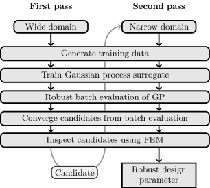
Figure 1: A schematic of the optimization procedure. First, the complete, wide domain is considered. Training data is generated and used to train a Gaussian process surrogate. Then, robust estimates of the design performance on the complete domain are obtained by calculating Monte Carlo integrals on the surrogate model. The best results are considered as candidates, which are inspected more closely using the FEM model. Here, we select the best result and use its parameters to narrow the complete domain to a much more focused domain. We use this narrow domain for a second pass through the pipeline to obtain robust design parameters, for a design which is insensitive to fabrication uncertainties. The complete procedure is described in more detail in Section 3.

The approach is founded on well understood Monte Carlo sampling [26, 27] and assumes knowledge about the type and extent of the deviations contained in the manufacturing processes parameters, such that we can construct a probability distribution to draw samples from, e.g., a parameter $p_{i}$ scatters according to a normal distribution with some mean $\mu_{i}$ and standard deviation $\sigma_{i}$, i.e., $p_{i}\sim\mathcal{N}(\mu_{i},\sigma_{i})$). As such, the presented approach leans towards branches of robust optimization called stochastic programming [28, 29] and scenario analysis [28]. A Gaussian process machine learning surrogate model [30] of the parameterized computer model is trained and used for the Monte Carlo sampling in lieu of the expensive model. This helps to effectively manage the computational burden normally imposed by Monte Carlo sampling procedures. An analysis of the percentiles of the results sampled from the Gaussian process is used to give a prediction of the results that can actually be expected from the device when manufactured in reality. We opt to optimize for the median, however, worst case optimizations with very small percentiles are also thinkable.

The approach presented in this article represents the background and the current state of development of a methodology that we have previously applied to create robust designs: In [31] a novel cavity design was first optimized using a Bayesian optimizer [32, 33]. The robustness of the parameter identified by the optimizer has then been assessed with a Monte Carlo sampling approach that was accelerated using Gaussian process surrogate models. In [34], a series of parameter candidates were determined using a Bayesian optimizer. A Gaussian process surrogate model was then trained in a region around each candidate. These Gaussian processes were used to find the most robust candidate by optimization. The objective function computed robust results by incorporating a large number of Monte Carlo samples that were drawn from a probability distribution informed by the assumed uncertainties of the manufacturing process. Other authors have published articles on robust optimization using Gaussian processes (under the term ’Kriging’) and Monte Carlo sampling [35, 36], where differences can be found, e.g., in the used optimization scheme (both publications employed a simulated annealing approach that additionally helped to parameterize the sample size of the Monte Carlo sampling).

This article extends these approaches by also considering the robustness of the parameters investigated in the initial candidate identification step. In [31, 34], this was done by a Bayesian optimizer, using the expensive forward model function, where only point values were calculated. In [31], the robustness was only assessed and not optimized, and, in [34], the robustness was not optimized across the complete parameter space.

We apply the method to the robust optimization of a photonic crystal nanobeam cavity based on cylindrical holes in an optical waveguide [37, 38], where the figure of merit we aim to maximize in a robust fashion is the Purcell enhancement, $F_{\mathrm{P}}$ [39]. Compared to the quality factor, $F_{\mathrm{P}}$ varies smoother across the parameter space (since it depends on both, quality factor and mode volume [39, 37]). The Purcell enhancement is computed by using scattering simulations with a dipole emitter modeling a point source, which is placed in the cavity and emits at an experimentally relevant wavelength.

The article is organized as follows: Section 2 provides details on the employed mathematical tools, such as Gaussian processes and Bayesian optimization. In Section 3, the optimization procedure is described in detail. In Section 4.1, the model of a photonic crystal nanobeam cavity is introduced. In Section 4.2, we apply the procedure for the optimization of the model of the photonic cystal nanobeam cavity, and also compare the obained results to a result found without restricting to a robust solution. Finally, Section 5 summarizes the findings.

2 Theory

The presented approach relies on Gaussian processes and Monte Carlo sampling techniques. The theoretical foundation for these methods is reviewed in the following.

2.1 Gaussian process regression

Gaussian processes (GPs) [30] are stochastic machine learning surrogate models that can be fit to numerical training data, i.e., inputs in the form of a set of $M$ positions $\bm{P}=\left[\bm{p}_{1},\dots,\bm{p}_{M}\right]^{\mathrm{T}}$ in some $N$-dimensional parameter space $\mathcal{X}\subset\mathbb{R}^{N}$, with each $\bm{p}_{m}\in\mathcal{X}$, and $M$ associated numerical values $\tilde{\bm{Y}}=\left[\tilde{y}_{1},\dots\tilde{y}_{M}\right]^{\mathrm{T}}$ where each $\tilde{y}_{m}\in\tilde{\mathcal{Y}}\subset\mathbb{R}$. After the GP has been trained on $\tilde{\bm{Y}}$ it can then be used as an approximator or predictor of the training data that can be evaluated at each point in $\mathcal{X}$. The training data is often generated by evaluating some (often expensive) parameterized process, e.g., a function $f:\mathcal{X}\to\tilde{\mathcal{Y}}$. The process is generally considered as a black box, and only few assumptions are made with respect to the data generated by it [32]. An important one is that in order to achieve a good fit the data should appear as if it could in principle have been drawn from some GP [32]. Otherwise a GP would not be able to model it accurately. One aspect of this is that we require the data set $\tilde{\bm{Y}}$ to (roughly) follow a normal distribution. A huge benefit of a GP is that it is typically much cheaper to evaluate than the process used to create the training data.

Mathematically, a GP is an infinite dimensional extension of a (finite dimensional) multivariate normal distribution [40]. They are defined on the continuous domain $\mathcal{X}$. While multivariate normal distributions are fully determined by a mean vector $\bm{\mu}$ and a positive (semi-)definite covariance matrix $\mathbf{\Sigma}$ [40], GPs are instead fully specified by a mean function $\mu:\mathcal{X}\to\mathbb{R}$ and a covariance kernel function $k:\mathcal{X}\times\mathcal{X}\to\mathbb{R}$ [30]. Common choices for these functions are a constant mean function $\mu(\bm{p})=\mu_{0}$ and a Matérn $\nicefrac{{5}}{{2}}$ kernel function [41], i.e.,

$$k(\bm{p},\bm{p}^{\prime})=\sigma_{0}\left(1+\sqrt{5}r+\frac{5}{3}r^{2}\right)\times\exp\left(-\sqrt{5}r\right)\,,$$ (1)

$$\text{with}\quad r=\sqrt{\sum_{i=1}^{N}\left(\frac{p_{i}-p_{i}^{\prime}}{l_{i}}\right)^{2}}\,.$$

These choices are also applied throughout this article. The quantity $r$ describes normalized distances between parameters $\bm{p}$ and $\bm{p}^{\prime}$. Like many other machine learning methods GPs are also controlled by means of hyperparameters [42, 43] (here prior mean value $\mu_{0}$, prior standard deviation $\sigma_{0}$ and length scales $l_{i}$ for each dimension of the training data $\tilde{\bm{Y}}$). However, in contrast to, e.g., deep neural networks [43], suitable values for the hyperparameters can be efficiently determined from the training data. The hyperparameters are chosen to maximize the likelihood of the training data [44].

The predictions of a GP are made in terms of a normal distribution for each point $\bm{p}_{\ast}\in\mathcal{X}$, i.e.,

$$\hat{f}(\bm{p}_{\ast})\sim\mathcal{N}(\overline{y}(\bm{p}_{\ast}),\sigma^{2}(\bm{p}_{\ast}))\,.$$ (2)

The hat notation is used to indicate a random variable. After the GP has been trained on training data, the predicted mean value $\overline{y}(\bm{p}_{\ast})$ approximates the training data and the predicted variance value $\sigma^{2}(\bm{p}_{\ast})$ describes how much the training data is expected to scatter around the predicted mean, given some choice of hyperparameters. For the predicted mean and variance values, we have

$$\overline{y}(\bm{p}_{\ast}) =\mu_{0}+\bm{k}^{\mathrm{T}}(\bm{p}_{\ast})\mathbf{K}^{-1}\left(\tilde{\bm{Y}}-\mu_{0}\cdot\mathbf{1}\right)\,,$$ (3)

$$\sigma^{2}(\bm{p}_{\ast}) =\sigma_{0}^{2}-\bm{k}^{\mathrm{T}}(\bm{p}_{\ast})\mathbf{K}^{-1}\bm{k}(\bm{p}_{\ast})\,,$$ (4)

with $\bm{k}(\bm{p}_{\ast})=\left[k(\bm{p}_{\ast},\bm{p}_{1}),\dots,k(\bm{p}_{\ast},\bm{p}_{M})\right]^{\mathrm{T}}$, $(\mathbf{K})_{ij}=k(\bm{p}_{i},\bm{p}_{j})$, and identity matrix $\mathbf{1}$.

2.1.1 Transformation based Gaussian processes for bounded data

Using data $\bm{Y}$ to train a GP that is clearly bounded to a specific subset of $\mathbb{R}$, e.g., $\bm{Y}=\left[y_{1},\dots,y_{M}\right]$ with $y_{m}\in\mathcal{Y}=\mathbb{R}^{+}$, can lead to problems associated with the predictions of the GP [45, 46]. Since the predictions of a GP are by definition unbounded [32, 43], they can sometimes exceed the support of the training data, i.e., the predicted variance region or even the predicted mean of the GP are assuming values not in $\mathcal{Y}$. This poses the question of how useful these predictions are. This problematic behavior is exacerbated if, e.g., a large amount of the training data is situated close to one side of $\mathcal{Y}$.

A possible way of dealing with this issue is by transforming the training data $\bm{Y}$ from its bounded domain $\mathcal{Y}$ to an unbounded co-domain $\tilde{\mathcal{Y}}$ with a bijective transformation function $g:\mathcal{Y}\to\tilde{\mathcal{Y}}$. The unbounded training data $\tilde{\bm{Y}}=\left[\tilde{y}_{1},\dots,\tilde{y}_{M}\right]^{\mathrm{T}}=\left[g(y_{1}),\dots,g(y_{M})\right]^{\mathrm{T}}=g(\bm{Y})$ can then be used to train the GP as described in Section 2.1, and the predictions made by the GP in the unbounded co-domain $\tilde{\mathcal{Y}}$ can then be transformed back to the bounded domain $\mathcal{Y}$ by applying the inverse transformation function $g^{-1}:\tilde{\mathcal{Y}}\to\mathcal{Y}$.

The training data used in this article is bounded to the domain $\mathcal{Y}=\mathbb{R}^{+}$ [39]. In order to transform this data we follow the approach taken in [34], which extends the approach taken in [45], and define a one sided piece-wise defined inverse transformation function $g^{-1}$ that maps from the unbounded co-domain to the bounded domain.

Training data between the lower bound of $y_{\mathrm{lower}}=0$ and some lower cut-off value $y_{\mathrm{lower,cutoff}}>y_{\mathrm{lower}}$ is transformed by means of a simple exponential function, i.e., by $g_{\mathrm{lower}}^{-1}(\tilde{y})=y_{\mathrm{lower}}+\exp\left(a_{\mathrm{lower}}(\tilde{y}-b_{\mathrm{lower}})\right)$.

Training data with $y\geq y_{\mathrm{lower,cutoff}}$ is transformed using an affine transformation, $g_{\mathrm{linear}}^{-1}(\tilde{y})=m_{\mathrm{linear}}\tilde{y}+b_{\mathrm{linear}}$. The steepness of the affine transformation is fixed to $m_{\mathrm{linear}}=1$ in accordance with [34]. It was observed that allowing variation of $m_{\mathrm{linear}}$ only led to a reduction in the predicted variance of the GP, and no improvement in the quality of the prediction [34]. This was considered as a form of overfitting. The parameter was therefore kept constant.

The two segments are matched such that they yield a continuously differentiable function $g^{-1}$. The transformation is controlled by the cut-off bound $y_{\mathrm{lower,cutoff}}$ and the position parameter of the exponential segment, $b_{\mathrm{lower}}$. The remainder of the transformation parameters can be calculated from these control parameters. The parameters $y_{\mathrm{lower,cutoff}}$ and $b_{\mathrm{lower}}$ are determined by means of a hyperparameter optimization [45].

2.2 Bayesian optimization

A very prominent application area for GPs is Bayesian optimization (BO) [32, 33, 44]. BO methods are a class of global sequential optimization methods that are known for being very efficient at optimizing expensive black box functions (expensive in terms of the consumed resources per evaluation) [47]. During the optimization, a GP is iteratively trained on observations of the black box function $f(\bm{p})$. At each iteration $M$ the predictions of the GP are used to generate a new sample candidate $\bm{p}_{M+1}$, that is used to evaluate $f(\bm{p})$ again. These new results are used to retrain the GP. New sample candidates are generated by maximizing a utility function $\alpha(\bm{p})$ that assigns usefulness to points in the parameter space for achieving the goal of the optimization, e.g., for maximizing or minimizing the optimized function. Here, we employ the expected improvement (EI) [47] with respect to the previously found smallest function value $f_{\mathrm{min}}=\min\{f(\bm{p}_{1}),\dots,f(\bm{p}_{M})\}$, i.e., calculate

$$\bm{p}_{M+1}=\underset{\bm{p}\in\mathcal{X}}{\arg\max}\,\alpha_{\mathrm{EI}}(\bm{p})\,,$$ (5)

$$\text{with}\quad\alpha_{\mathrm{EI}}(\bm{p})=\mathrm{E}\left[\min\left(0,f_{\mathrm{min}}-\hat{f}(\bm{p})\right)\right]\,.$$ (6)

This iterative procedure is continued until a provided optimization is exhausted. The BO method applied in this article is implemented in the analysis and optimziation toolkit [33] of the solver JCMsuite [6].

2.3 Robust design evaluation with Monte Carlo approximation

Monte Carlo methods [26, 27] are powerful approaches that can be used to tackle statistical problems that are difficult to solve analytically. They generally involve a large number of random numbers from some probability distribution that are used to perform computations. The results are aggregated and can be further used to perform, e.g., a statistical analysis [48]. Monte Carlo methods can also be applied to assess the robustness of a design for a device under given uncertainties in the devices parameters [35, 36].

Assume that we constructed a forward model function $f(\bm{p})$ which resembles the device that we want to manufacture in reality. Using a BO method, we have identified a model parameter $\bm{p}_{\mathrm{opt}}$ for which $f(\bm{p})$ assumes a maximum. If we were able to manufacture the device in reality, even assuming that the model perfectly captures its characteristics and the underlying physics, we will usually not be able to achieve the optimized model function value $f(\bm{p}_{\mathrm{opt}})$. This is because typically the device parameters realized in the manufacturing process are associated with some uncertainty and scatter around $\bm{p}_{\mathrm{opt}}$ to a certain extent [49].

Using a Monte Carlo approach, we can quantify the actually realized performance of the device. For this, we assume that the parameters that are realized by the manufacturing process scatter according to some manufacturing distribution $\mathcal{D}$ that is derived from the uncertainties associated with the manufacturing process, and then draw a large number of $M_{\mathrm{device}}$ random samples ${\bm{P}}_{\mathrm{device}}=\{{\bm{p}}_{1},\dots,{\bm{p}}_{M_{\mathrm{device}}}\}$ from this distribution. We use these to evaluate the devices model function, i.e., calculate ${\bm{Y}}=\{f({\bm{p}}_{1}),\dots,f({\bm{p}}_{M_{\mathrm{device}}})\}$. Since the samples ${\bm{P}_{\mathrm{device}}}$ are random numbers, the function values ${\bm{Y}}$ are also random numbers that follow some statistical distribution.

As an illustrative example for such a manufacturing distribution, we choose a $N$-dimensional multivariate normal distribution [48], e.g., $\mathcal{D}=\mathcal{N}(\bm{p}_{\mathrm{device}},\mathbf{\Sigma}_{\mathrm{manuf}})$, with diagonal covariance matrix $\mathbf{\Sigma}_{\mathrm{manuf}}={\rm diag}(\sigma_{1}^{2},\dots,\sigma_{N}^{2})$. In doing this, we assume that the manufacturing process is set up to yield devices that are on average described by the parameter $\bm{p}_{\mathrm{device}}$, but due to the assumed uncertainties $\sigma^{2}_{i}$ in the manufacturing process the actually realized devices all scatter around the mean according to the covariance matrix $\mathbf{\Sigma}_{\mathrm{manuf}}$. By assuming a diagonal covariance matrix, we imply that the fabrication uncertainties of the individual parameters $p_{\mathrm{device},i}$ are not correlated in any way [48].

To quantify the devices performance under manufacturing uncertainty, we can look, e.g., at the expectation value of ${\bm{Y}}$ [27]

$$\mathrm{E}\left[{\bm{Y}}\right]=\frac{1}{M_{\mathrm{device}}}\sum_{m=1}^{M_{\mathrm{device}}}f({\bm{p}}_{m})$$ (7)

and its variance [27]

$$\mathrm{Var}\left[{\bm{Y}}\right]=\frac{1}{M_{\mathrm{device}}}\sum_{m=1}^{M_{\mathrm{device}}}\left(f({\bm{p}}_{m})-\mathrm{E}\left[{\bm{Y}}\right]\right)^{2}.$$ (8)

For highly symmetric distributions, the expectation value and variance are good measures for the quantification of the devices performance. In some cases, however, ${\bm{Y}}$ can show large amounts of skew. These distributions are difficult to describe using $\mathrm{E}\left[{\bm{Y}}\right]$ and $\mathrm{Var}\left[{\bm{Y}}\right]$. A better description can be achieved by calculating certain percentiles of the distribution of ${\bm{Y}}$ that relate the expected performance of the device to the expectation value and variance of a well known reference distribution. Conveniently, we draw parallels to a normal distribution $\mathcal{N}(\mu,\sigma^{2})$. Here, the 50’th percentile or median $P_{50}$ relates to the mean $\mu$ of the normal distribution and the 16’th and 84’th percentiles $P_{16}$ and $P_{84}$ to the lower standard deviation $\mu-\sigma$ and upper standard deviation $\mu+\sigma$, respectively.

As such, we use these percentiles to construct analogs to the lower and upper standard deviation for the potentially skewed distribution of ${\bm{Y}}$,

$$\sigma_{-}({\bm{Y}}) =P_{50}({\bm{Y}})-P_{16}({\bm{Y}})\quad\text{and}$$ (9)

$$\sigma_{+}({\bm{Y}}) =P_{84}({\bm{Y}})-P_{50}({\bm{Y}})\,,$$ (10)

respectively. The median $P_{50}({\bm{Y}})$ is related to the expectation value.

Expectation values calculated using Monte Carlo methods get more accurate the more samples are used. An often used estimate for the error associated with the expectation value of ${\bm{Y}}$ is given as [27]

$$\sigma_{\mathrm{MC}}\approx\sqrt{\frac{\mathrm{Var}\left[{\bm{Y}}\right]}{M}}\,,$$ (11)

which tends toward zero as $M$ tends to infinity. We assume that we can apply this error measure to the percentile based approach employed by us.

Thus, using the random sample ${\bm{P}}$ to compute random forward model function values ${\bm{Y}}$, we can give an estimate for the realizable performance of the device as

$$\overline{f}=\left(P_{50}({\bm{Y}})\pm\sigma_{\mathrm{MC}}\right)_{\sigma_{-}({\bm{Y}})}^{\sigma_{+}({\bm{Y}})}\,.$$ (12)

This procedure can be incorporated into an (expensive) optimziation procedure if the mean of the manufacturing distribution, $\bm{p}_{\mathrm{device}}$, is iteratively chosen by an optimization method, e.g., by the BO method described earlier.

3 Robust design optimization procedure

While being conceptionally relatively simple, robust optimization of the model function $f(\bm{p})$ directly with the approach outlined in Section 2.3 is still difficult from a computational resources standpoint, since it involves evaluating the expensive model function a large number of times. Here, we are dealing with a few issues that compound themselves into a very challenging task.

On one hand the size of optimization domain has to be considered. Without any prior information for the model parameters $\bm{p}$ it is difficult to motivate a particular choice of limited parameter range. Instead, it is desirable to investigate large intervals in each of the problems parameter dimensions. Performing this in an unrobust fashion is already a challenging task [50].

On the other hand, in order to obtain a robust estimate for a given parameter the model function $f(\bm{p})$ has to be evaluated for many points in the vicinity of $\bm{p}$, as detailed in Section 2.3. This increases the computational cost for each considered point in the parameter space by a factor of $M_{\mathrm{device}}$.

The procedure presented in the following aims to resolve these issues. It is centered around cheap to evaluate Gaussian process surrogate models. This helps to efficiently manage the computational burden imposed by a robust design optimization. The predictions of this GP surrogate are used during the application of an iterative Monte Carlo sampling technique detailed in Algorithm 1. In it, we go through a series of five steps in two successive passes and at the end obtain a parameter candidate that is predicted to be robust against some assumed manufacturing uncertainties.

Algorithm 1 An iterative Monte Carlo sampling procedure to determine a robust device performance estimate, by obtaining predictions from a trained GP surrogate at positions drawn from some manufacturing distribution $\mathcal{D}$.

function RobustEstimate(Predicted GP mean $\overline{y}(\bm{p})$ (Equation 3), predicted GP variance $\sigma^{2}(\bm{p})$ (Equation 4), manufacturing distribution $\mathcal{D}$)

     $\sigma_{\mathrm{rel,MC}}=\infty$ $\triangleright$ Initialize the relative MC error.

     $N_{\mathrm{tot}}=0$ and $N_{\mathrm{min}}$ = $50\,000$ $\triangleright$ Initialize the number of samples drawn.

     ${\bm{Y}}_{\mathrm{tot}}=\emptyset$ and ${\bm{S}}_{\mathrm{tot}}=\emptyset$ $\triangleright$ Initialize the sets of GP mean and variance observations.

     while $(\sigma_{\mathrm{rel,MC}}\geq${10}^{-3}$$ and $N_{\mathrm{tot}}<N_{\mathrm{min}})$ do

         ${\bm{P}}\sim\mathcal{D}$ and $N_{\mathrm{tot}}=N_{\mathrm{tot}}+$1000$$ $\triangleright$ Draw $1000$ random samples from manufacturing distribution.

         ${\bm{Y}}=\overline{y}({\bm{P}})$ and ${\bm{S}}=\sigma^{2}({\bm{P}})$ $\triangleright$ Use samples to calculate predicted GP mean and variance values (Equations 3 and 4).

         ${\bm{Y}}_{\mathrm{tot}}={\bm{Y}}_{\mathrm{tot}}\cup{\bm{Y}}$ and ${\bm{S}}_{\mathrm{tot}}={\bm{S}}_{\mathrm{tot}}\cup{\bm{S}}$ $\triangleright$ Collect mean and variance observations.

         $\sigma_{\mathrm{rel,MC}}=\sigma_{\mathrm{MC}}({\bm{Y}}_{\mathrm{tot}})/P_{50}({\bm{Y}}_{\mathrm{tot}})$ $\triangleright$ Check convergence of MC sampling (using Equation 11).

     end while

     $\sigma_{\mathrm{GP}}^{2}=P_{50}({\bm{S}}_{\mathrm{tot}})$ $\triangleright$ Use variance observations to estimate error introduced by GPs.

     $\sigma_{\mathrm{Median}}=\sqrt{\sigma_{\mathrm{GP}}^{2}+\sigma_{\mathrm{MC}}^{2}}$ $\triangleright$ Calculate uncertainty for the predicted device performance (using Equation 11.)

     $\sigma_{-}({\bm{Y}}_{\mathrm{tot}})=P_{50}({\bm{Y}}_{\mathrm{tot}})-P_{16}({\bm{Y}}_{\mathrm{tot}})$ $\triangleright$ Use mean observations to calculate lower …

     $\sigma_{+}({\bm{Y}}_{\mathrm{tot}})=P_{84}({\bm{Y}}_{\mathrm{tot}})-P_{50}({\bm{Y}}_{\mathrm{tot}})$ $\triangleright$ …and upper standard deviation for the predicted device performance.

     return $\left(P_{50}({\bm{Y}}_{\mathrm{tot}})\pm\sigma_{\mathrm{Median}}\right)^{\sigma_{+}({\bm{Y}}_{\mathrm{tot}})}_{\sigma_{-}({\bm{Y}}_{\mathrm{tot}})}$ $\triangleright$ Return robust device performance estimate.

end function

In the first step, training data is generated by evaluating the considered model function $f(\bm{p})$ at many different positions across the parameter space. In step two, a GP surrogate model for bounded data is fit to the training data. In step three, the trained GP surrogate is employed to generate robust estimates of the model function output at many positions in the computational domain. The quality of these estimates scales inversely with the dimensionality of the parameter space and the size of the investigated domain. In step four, the best robust estimate(s) found in step three is (are) converged using a Bayesian optimizer. Finally, in step five, the converged candidates are inspected and their robustness is verified using the expensive forward model function $f(\bm{p})$.

Using two distinct passes helps dealing with the size of the optimization domain. In the first pass, a very large domain is considered in a rather coarse fashion. The parameter candidate generated here only serves to define a much smaller domain to be investigated in the second pass. The parameter candidate generated by the second pass finally is predicted to be robust against the assumed manufacturing uncertainties.

There is, however, no guarantee that we might overlook a very good candidate, since the parameter space in the first pass can be very large when compared to the length scales on which the forward model function $f(\bm{p})$ varies. This is a computational cost problem, that can be resolved, e.g., by partitioning the computational domain and then investigating each of these partitions in a more refined way. This approach does, however, not scale that well for high dimensional problems, which is a direct manifestation of the curse of dimensionality [51].

In addition to the optimized forward model function $f(\bm{p})$, the procedure also requires an optimization domain and a set of assumed manufacturing uncertainties. The uncertainties are used to construct manufacturing distributions employed during the robust optimization. Here, we limit our considerations to simple multivariate normal distributions [48] with diagonal covariance matrix $\mathbf{\Sigma}_{\mathrm{manuf}}$. The approach is easily extended to more complex distributions.

The individual steps are discussed in more detail in the following.

3.1 Step 1: Generating training data

Given a domain $\mathcal{Q}_{\mathrm{train}}\subset\mathcal{X}$, a forward model function $f(\bm{p})$ that is to be optimized in a robust fashion, and the assumed manufacturing uncertainties $\sigma_{d_{i}}$ for each parameter, we generate a large number of training data points in $\mathcal{Q}_{\mathrm{train}}$. The manufacturing uncertainty imposes minimum-size-requirement on the domain $\mathcal{Q}_{\mathrm{train}}$. It must be possible to position a constructed manufacturing normal distribution $\mathcal{D}$ in a way that, when drawing many random samples from it, a very large portion of these samples are in $\mathcal{Q}_{\mathrm{train}}$. We will elaborate on this in Section 3.3.

Samples $\bm{P}_{\mathrm{train}}$ are drawn from a Sobol sequence [52, 53] scaled to $\mathcal{Q}_{\mathrm{train}}$ and used to evaluate $f(\bm{p})$, thereby generating the training data $\bm{Y}_{\mathrm{train}}=f(\bm{P}_{\mathrm{train}})$. Sobol sequences are low-discrepancy sequences of points in a $N$-dimensional space that cover the space somewhat evenly, provided that the number of used samples equals to a natural power of two [54]. Because of the costs associated with the evaluation of the forward model function and because the performance of GPR decreases drastically if a very large number of samples are used to train it [43], we draw $2^{12}=$4096$$ samples from the Sobol sequence. Depending on the dimensionality and size of the parameter space of the model, this choice may result in a sparse sampling of the space. For the dimensionalities considered by us, also, e.g., in [34], this number was demonstrated to be sufficient.

Some filtering of $\bm{Y}_{\mathrm{train}}$ for the next step can be beneficial, since a GP generally assumes that the data used to train it could have been drawn from some GP, i.e., it is normally distributed [32]. As such, extreme outliers in $\bm{Y}_{\mathrm{train}}$ should be removed to assure that the predictions of the trained GP are a good approximation of the function $f(\bm{p})$.

3.2 Step 2: Training the GP surrogate

The (potentially filtered) bounded training data $\bm{Y}_{\mathrm{train}}$ and associated samples $\bm{P}_{\mathrm{train}}$ are used to train the GP surrogate model for bounded data described in Section 2.1.1. This involves finding all the hyperparameters for the transformation function $g$ that is used to transform the bounded training data to an unbounded co-domain for training the GP, and transforming the predictions of the GP back to the bounded domain by applying $g^{-1}$. Depending on the number of training data points and on the size of the domain $\mathcal{Q}_{\mathrm{train}}$, this surrogate can be a coarse or fine approximation of the forward model function $f(\bm{p})$ on the domain $\mathcal{Q}_{\mathrm{train}}$.

3.3 Step 3: Batch calculation of robust estimates

A large number of $M_{\mathrm{eval}}$ samples $\bm{P}_{\mathrm{eval}}=\left[\bm{p}_{1},\dots,\bm{p}_{M_{\mathrm{eval}}}\right]$ are drawn from a Sobol sequence that is scaled to the domain $\mathcal{Q}_{\mathrm{eval}}\subset\mathcal{Q}_{\mathrm{train}}$. These are used to construct various manufacturing normal distributions $\mathcal{D}_{i}=\mathcal{N}(\bm{p}_{i},\mathbf{\Sigma}_{\mathrm{manuf}})$. In conjunction with the trained GP surrogate on $\mathcal{Q}_{\mathrm{train}}$, they are used to generate robust estimates of the forward model function $f(\bm{p})$, by applying Algorithm 1.

The domain $\mathcal{Q}_{\mathrm{eval}}$ is reduced in size by three standard deviations in each direction and each parameter when compared to $\mathcal{Q}_{\mathrm{train}}$. This is done to assure that the samples drawn from the manufacturing distribution $\mathcal{D}_{i}$ during the application of Algorithm 1 are located in regions where the predictions of the GP surrogate are informed by training data. Consider a parameter $\bm{p}_{\mathrm{corner}}\in\mathcal{Q}_{\mathrm{eval}}$ which sits in a corner of the domain $\mathcal{Q}_{\mathrm{eval}}$. Determining a robust estimate for this parameter means drawing a large number of samples from the normal distribution $\mathcal{N}(\bm{p}_{\mathrm{corner}},\mathbf{\Sigma}_{\mathrm{manuf}})$. By the properties of normal distributions, approximately $99.7\text{\,}\mathrm{\char 37\relax}$ of all drawn samples will be contained in a hypersphere with a radius of three standard deviations defined by the covariance matrix $\mathbf{\Sigma}_{\mathrm{manuf}}$ [40]. Since the training domain $\mathcal{Q}_{\mathrm{train}}$ of the GP surrogate is three standard deviations larger, this means that more than $99.7\text{\,}\mathrm{\char 37\relax}$ of all predictions will be informed by training data. Moving the center of the normal distribution outside of $\mathcal{Q}_{\mathrm{eval}}$ reduces this fraction.

Algorithm 1 extends the sampling procedure described in Section 2.3 by one aspect. Instead of sampling the forward model function $f(\bm{p})$ directly, a GP surrogate model of the function is sampled. GP surrogates are always associated with some uncertainty in the prediction, quanfitied by the predicted variance, Equation 4. This variance prediction can be utilized to extend Equation 12 and to give an estimate for the uncertainty of the predicted robust estimate, too. For this, the random samples ${\bm{P}}$ drawn during application of Algorithm 1 are used to generate predicted variances ${\bm{S}}=\sigma^{2}({\bm{P}})$. The median of these variance samples $\sigma_{\mathrm{GP}}^{2}=P_{50}({\bm{S}})$ is used together with the Monte Carlo error, Equation 11, to give a combined predicted uncertainty as

$$\sigma_{\mathrm{Median}}=\sqrt{\sigma_{\mathrm{GP}}^{2}+\sigma_{\mathrm{MC}}^{2}}\,.$$ (13)

Using this we can give the estimate of the realizable device performance as

$$\overline{f}=\left(P_{50}({\bm{Y}})\pm\sigma_{\mathrm{Median}}\right)_{\sigma_{-}({\bm{Y}})}^{\sigma_{+}({\bm{Y}})}\,.$$ (14)

Conventionally, one would not use a batch evaluation of the robust estimate, but rather employ some form of optimization method to scan the parameter space. We have, however, observed that even optimization methods that are designed for global optimization (we used BO) had issues coping with the size of the investigated domain in the first pass.

This is associated with two issues in particular. First, the BO method tends to exploit promising values rather than exploring the parameter space. While this approach may work in the second pass through the pipeline, in the first pass, it spends a large number of evaluations that could much better be spent exploring the parameter space. And second, this exploitation of promising values was tied to collecting many training data points. At each BO iteration a matrix has to be inverted that scales with the number of training data points [43, 32]. As such, the BO method becomes very slow after many samples have been investigated.

These issues could in principle be resolved by using a conventional optimization method, such as L-BFGS-B [55], albeit at the expense of the global optimization property of the method. To therefore reliably cover a wide area in the parameter space one could employ a random multi start approach [56]. However, we deemed it more efficient to sample well known locations in the parameter space directly.

The results obtained using the batch approach are sorted by their predicted performance. Good results that are in very close proximity to other good results are filtered, such that only the best results from a cluster is kept. A limited number of best filtered results are then investigated in the next step.

3.4 Step 4: Converging robust design candidates

The filtered results were each used as starting point for a Bayesian optimizer, by pre-training the optimization method on them. This pre-training has nudged the optimizer into exploiting the area surrounding the filtered result. The BO method iteratively chose the mean $\bm{p}$ of the manufacturing normal distribution $\mathcal{D}=\mathcal{N}(\bm{p},\mathbf{\Sigma}_{\mathrm{manuf}})$ used during the application of Algorithm 1 on the trained GP surrogate. As in the previous step, the domain $\mathcal{Q}_{\mathrm{eval}}$ is used as optimization domain.

3.5 Step 5: Inspection and verification of converged candidates

This step is primarily important for the first pass, as it is used to determine ranges in the parameter space to investigate more closely. It is not strictly necessary for the second pass, but can still be interesting to verify the predictions of the GP surrogates and check that the results are sensible.

The predicted results for the converged parameters found in the previous step are verified using the expensive forward model function $f(\bm{p})$. A limited number of random samples ${\bm{P}}_{\mathrm{test}}$ are drawn from the manufacturing distribution centered on the converged robust design candidates and used to evaluate $f(\bm{p})$. The median of the results is calculated. In order to select a parameter region for the second pass, the best median forward model result is selected.

Note that the number of samples investigated in the second pass should be large enough such that the Monte Carlo error associated with the final converged results does not dominate these [26, 27].

4 Application

4.1 Model of a photonic nanobeam cavity

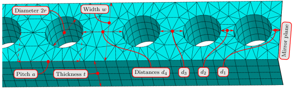
Figure 2: An exemplary parameterization of the cavity. All cavity parameters are illustrated by means of red arrows. The hole diameters $2r$, as well as cavity width $w$, pitch $a$, and thickness $t$ are determined by optimizing the crystal unit cell. The distances $d_{1}$ to $d_{4}$ are chosen to yield a cavity whose Purcell factor $F_{\mathrm{P}}$ is robust under a given fabrication uncertainty for the distances.

To demonstrate the method, we optimize a hole based photonic crystal nanobeam cavity [37, 38] in a robust way. The cavity is an open system, i.e., it is described by resonances [57, 58]. The maximized target quantity is the Purcell enhancement $F_{\mathrm{P}}$ of the cavity, which is given by the quotient of the total emission of a dipole embedded in the cavity and the dipole emission in homogeneous bulk material [39, 59]. The dipole emits at a wavelength of $1550\text{\,}\mathrm{nm}$, i.e., in the telecom C-band wavelength [60]. The model is set up and solved using the Maxwell solver JCMsuite which is based on the finite-element method [6].

The photonic crystal nanobeam cavity is constructed by repeating a finite number of unit cells periodically along a single dimension. The unit cells are modeled as a rectangular block of silicon with thickness $t$, width $w$, and length or pitch $a$. A hole through the block with diameter $2r$ is positioned in the center of the $a$-$w$ plane [37]. The band structure of the photonic crystal contains some fundamental dielectric band $\lambda_{\mathrm{diel}}$ and a next higher air band $\lambda_{\mathrm{air}}$, which can form a band gap [37]. In order to create a cavity mode within this crystal, the location $\overline{\lambda}_{\mathrm{gap}}$ and size $\Delta\lambda_{\mathrm{gap}}$ of this band gap within the band structure must be controlled [37].

We can then create a resonant cavity by introducing a defect at some position of the crystal, which breaks up the periodicity of the crystal. A very simple way of doing this is by, e.g., varying the distance between two of the holes. This variation modifies the amount of material in the crystal at that position and therefore also the band structure, which can allow for the emergence of a resonance mode in the region of the defect. Ideally, due to the different band structure, this resonance mode can not propagate inside the periodic region. The periodic region acts thus as a mirror for the resonance mode. A more thorough treatment of the topic can be found in the literature [37].

The task at hand is two fold. First, the parameters of the periodic unit cell, i.e., the pitch $a$, the width $w$, the thickness $t$, and the diameter $2r$, must be chosen such that the periodic region serves as an effective mirror for a desired resonance mode, by disallowing its propagation entirely. And, second, degrees of freedom have to be introduced to parameterize the crystal defect, and these have to be chosen such that the desired resonance mode emerges in the defect region.

The parameters of the unit cell are chosen to create a photonic crystal with a very large band gap centered around (or close to) the desired wavelength of $1550\text{\,}\mathrm{nm}$. For this, a Bayesian optimizer is used to minimize the objective function

$$b(\bm{q})=-1\cdot\frac{\Delta\lambda_{\mathrm{gap}}(\bm{q})}{|\overline{\lambda}_{\mathrm{gap}}(\bm{q})-$1550\text{\,}\mathrm{nm}$|}\,,$$ (15)

$$\text{with}\quad\Delta\lambda_{\mathrm{gap}}(\bm{q})=\lambda_{\mathrm{diel}}-\lambda_{\mathrm{air}}$$

$$\text{and}\quad\overline{\lambda}_{\mathrm{gap}}(\bm{q})=\left(\lambda_{\mathrm{diel}}+\lambda_{\mathrm{air}}\right)/2\,,$$

$$\text{where}\quad\bm{q}=\left[a,w,t,2r\right]^{\mathrm{T}}\,.$$

The fundamental dielectric and next higher air mode, $\lambda_{\mathrm{diel}}$ and $\lambda_{\mathrm{air}}$, respectively, are calculated by solving resonance problems. The objective functions $b(\bm{q})$ output becomes very small if the gap in the band structure $\Delta\lambda_{\mathrm{gap}}(\bm{q})$ becomes very large and the center of the gap in the band structure $\overline{\lambda}_{\mathrm{gap}}(\bm{q})$ is very close to the target wavelength of $1550\text{\,}\mathrm{nm}$. We find that a unit cell with pitch $a=$560\text{\,}\mathrm{nm}$$, width $w=$620\text{\,}\mathrm{nm}$$, thickness $t=$395\text{\,}\mathrm{nm}$$, and a hole diameter of $2r=$336\text{\,}\mathrm{nm}$$ has a band gap of $\Delta\lambda_{\mathrm{gap}}\approx$214\text{\,}\mathrm{nm}$$, centered around a wavelength of $\overline{\lambda}_{\mathrm{gap}}\approx$1554\text{\,}\mathrm{nm}$$. The fundamental dielectric mode has a wavelength of $\lambda_{\mathrm{diel}}\approx$1661\text{\,}\mathrm{nm}$$ and the next higher air mode a wavelength of $\lambda_{\mathrm{air}}\approx$1447\text{\,}\mathrm{nm}$$.

The photonic crystal nanobeam cavity is created by periodically repeating 13 unit cells in the computational domain. We further consider a mirror symmetric setup, i.e., we treat one side of the computational domain as a mirror plane. This effectively doubles the number of unit cells in the device. For the introduction and variation of the defect in the periodic structure, we consider the mirror plane, i.e., the center of the photonic crystal. Here, we allow the distances between the four innermost holes $d_{4}$, $d_{3}$, and $d_{2}$, as well as the distance from the first hole to the mirror plane, $d_{1}$, to vary. As such, we consider the four distance parameters $\bm{p}=\left[d_{1},d_{2},d_{3},d_{4}\right]$ for parameterization of the defect. The cavity consists of 10 mirror cells and 3 cavity cells on each side of the mirror plane. An excerpt of the geometrical layout of the cavity is depicted in Figure 2.

The Purcell enhancement $F_{\mathrm{P}}$ of this structure is calculated by means of scattering simulations [6], in which a dipole with an emission wavelength of $\lambda_{\mathrm{dipole}}=$1550\text{\,}\mathrm{nm}$$ is placed in the mirror plane, in the center of the waveguide material.

4.2 Robust design optimization of the nanobeam cavity

We have performed a robust optimization of the photonic crystal nanobeam cavity described in Section 4.1. During the optimization, we considered the cavity parameters $d_{1}$ to $d_{4}$ on the domain given in Table 1.

Design parameter	Parameter range
$d_{1}$	$\left[56,616\right]\,$\mathrm{nm}$$
$d_{2}$	$\left[56,616\right]\,$\mathrm{nm}$$
$d_{3}$	$\left[56,616\right]\,$\mathrm{nm}$$
$d_{4}$	$\left[56,616\right]\,$\mathrm{nm}$$

Table 1: The complete investigated design space, $\mathcal{Q}_{\mathrm{train,first}}$. This domain is used as a basis for the first pass of the optimization process described in Figure 1.

For each of the $d_{i}$, we assumed a manufacturing uncertainty of $\sigma_{d_{i}}=$16.8\text{\,}\mathrm{nm}$$ and no correlation between the $d_{i}$. This means that the combined manufacturing uncertainty can be modeled by a diagonal covariance matrix $\mathbf{\Sigma}_{\mathrm{manuf}}={\rm diag}(\sigma_{d}^{2},\sigma_{d}^{2},\sigma_{d}^{2},\sigma_{d}^{2})$. The unit cell parameters $a$, $w$, $t$, and $2r$ were kept constant and, for the sake of this demonstration, assumed not to be associated with any manufacturing uncertainty.

The following analysis closely follows the description given in Section 3 and the schematic in Figure 1. First, in a coarse pass, a candidate region was identified which shows a promising range of Purcell enhancements that allow for a robust solution under the assumed manufacturing uncertainties. This candidate region was then investigated more closely in a narrow and more refined second pass. Here, a parameter set was determined which maximizes the Purcell enhancement in a robust fashion such that moderate variations of the parameters yield similar Purcell enhancements. Such a result is much easier to realize in a manufacturing environment.

We used transformation based GPs since we expected that a very large number of training data values were very close to $0$, because the Purcell enhancement can be assumed to be very small for large portions of the parameter space.

4.2.1 First pass: candidate selection

A set of $4096$ parameters $\bm{P}_{\mathrm{train,first}}$ was drawn from a Sobol sequence for the domain $\mathcal{Q}_{\mathrm{train,first}}$ given in Table 1. These were used to generate training data $\bm{Y}_{\mathrm{train,first}}=f(\bm{P}_{\mathrm{train,first}})$ from the FEM model for the photonic crystal nanobeam cavity. The training data was inspected and data points with large values with $F_{\mathrm{P}}>50$ were removed. This applied to only two data points. The reason for this filtering is that a GP assumes training data that could in principle have been drawn from some GP, i.e., is normally distributed. Assuming that $\bm{Y}_{\mathrm{train,first}}$ roughly follows a normal distribution, values larger than $F_{\mathrm{P}}=50$ appeared uncharacteristically large. We will return to the largest value just removed from the data set in Section 4.3.

The remaining $4094$ data points were used to train a transformation based GP surrogate of the forward model function on the domain $\mathcal{Q}_{\mathrm{train,first}}$. Note that, due to the number of training points and the volume of the domain, this GP is a relatively coarse approximation of $f(\bm{p})$.

The trained GP was used to generate a large set of robust estimates of the Purcell enhancement. These robust estimates were calculated by applying Algorithm 1 for different manufacturing distributions $\mathcal{D}$. In accordance with the assumed manufacturing uncertainties $\sigma_{d_{i}}$, these were all normal distributions, i.e., $\mathcal{D}=\mathcal{N}(\bm{p},\mathbf{\Sigma}_{\mathrm{manuf}})$, which differed only in the mean $\bm{p}$ of the distributions. To quickly and efficiently cover the parameter space, we drew $4096$ samples to be used as mean values $\bm{p}$ from a Sobol sequence in the domain $\mathcal{Q}_{\mathrm{eval,first}}\subset\mathcal{Q}_{\mathrm{train,first}}$. The robust estimates were sorted by magnitude. Good values in close proximity (we used $d_{ij}=\lVert\bm{p}_{i}-\bm{p}_{j}\rVert<0.25$ as criterion) were filtered such that only the largest robust estimate was kept.

The six largest filtered results were each converged with a Bayesian optimizer. The objective function optimized was Algorithm 1, where the mean $\bm{p}$ of the manufacturing distribution was iteratively chosen to maximize the robust Purcell enhancement. Each of the six filtered results from the previous step were individually used as starting points for the optimization. It was found that two of the six candidates consistently converged into the same optimum, leaving five distinct candidates.

To identify the most promising parameter to inspect in the second pass, $64$ samples were drawn from appropriate manufacturing distributions $\mathcal{D}$ centered around each of the five candidates. These were used to evaluate the FEM model. We calculated the median of the calculated Purcell enhancements and selected the candidate with the highest value. Here, the parameter $\bm{p}_{\mathrm{opt,first}}=\left[428.6,282.5,369.5,253\right]\,$\mathrm{nm}$$ was selected for a more thorough inspection in the second pass. Taking the very coarse nature of the surrogate into account, we have seen a reasonable agreement between the results obtained using the predictions made by the GP surrogate (median of $9.4$) and the FEM model (median of $2.3$).

4.2.2 Second pass: robust optimization of candidates

The second, more refined pass was centered on the parameter $\bm{p}_{\mathrm{opt,first}}=\left[428.6,282.5,369.5,253\right]\,$\mathrm{nm}$$ identified in the first pass. A set of $4096$ training data points were generated on a domain spanning a total of ten standard deviations in each dimension, i.e., the domain $\mathcal{Q}_{\mathrm{train,second}}$ listed in Table 2.

Design parameter	Parameter range
$d_{1}$	$\left[344.6,512.6\right]\,$\mathrm{nm}$$
$d_{2}$	$\left[198.5,366.5\right]\,$\mathrm{nm}$$
$d_{3}$	$\left[285.5,453.5\right]\,$\mathrm{nm}$$
$d_{4}$	$\left[169,337\right]\,$\mathrm{nm}$$

Table 2: After a promising design candidate was found at $\bm{p}_{\mathrm{opt,first}}=\left[428.6,282.5,369.5,253\right]\,$\mathrm{nm}$$, the model was investigated more closely in this domain $\mathcal{Q}_{\mathrm{train,second}}$ centered around the value. This domain was used as a basis for the second pass of the optimization process described in Figure 1. This is a ten standard deviation hypercube centered around $\bm{p}_{\mathrm{opt,first}}$.

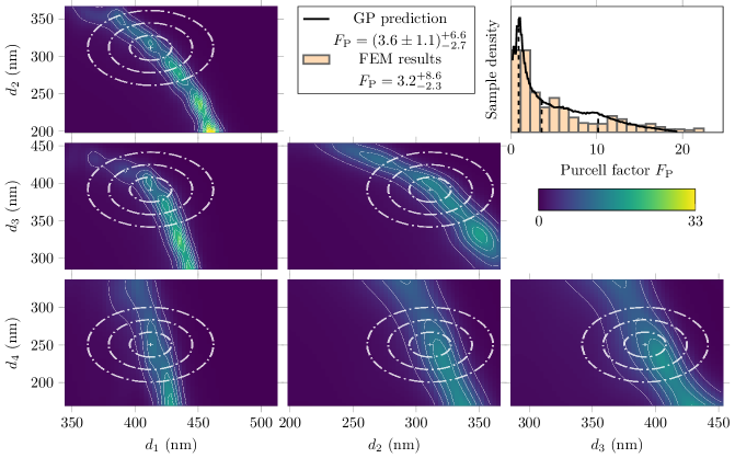
Figure 3: The function value landscape around the robust design parameter $\bm{p}_{\mathrm{robust}}=\left[412,311.5,392,250.3\right]\,$\mathrm{nm}$$ (marked with a white cross). The white ellipses around the white cross indicate (from smallest to largest) the $1\sigma$, $2\sigma$, and $3\sigma$ percentiles of the manufacturing distribution, which was assumed to be a multivariate normal distribution. The covariance matrix of this multivariate normal distribution was chosen to be $\mathbf{\Sigma}_{\mathrm{manuf}}={\rm diag}(\sigma_{d}^{2},\sigma_{d}^{2},\sigma_{d}^{2},\sigma_{d}^{2})$ with $\sigma_{d}=$16.8\text{\,}\mathrm{nm}$$. Applying Algorithm 1 in conjunction with a trained surrogate model allowed us to efficiently determine that a manufacturing process that produces devices according to a normal distribution with $\mathcal{N}(\bm{p}_{\mathrm{robust}},\mathbf{\Sigma}_{\mathrm{manuf}})$ yields devices with an expected Purcell enhancement $\overline{F}_{\mathrm{{P}}}=(3.6\pm 1.1)_{-2.7}^{+6.6}$. Verification using the FEM model showed that $\overline{F}_{\mathrm{P}}=3.2_{-2.3}^{+8.6}$. Both results are shown in the top right sub figure.

These $\bm{P}_{\mathrm{train,second}}$ were again drawn from a Sobol sequence and used to evaluate the FEM model with, thereby generating $\bm{Y}_{\mathrm{train,second}}=f(\bm{P}_{\mathrm{train,second}})$. These results were inspected to detect extreme outliers similar to the first pass.

Because none were found, all $4096$ data points were used for training the transformation based GP. The training data spans a much smaller domain, as such the resulting surrogate can be considered a much more accurate approximation of the FEM model $f(\bm{p})$.

A large set of robust estimates of the Purcell enhancements were generated by using Algorithm 1 in conjunction with the finer surrogate trained. Similar to the first pass, $4096$ different normal distributions centered on points $\bm{p}\in\mathcal{Q}_{\mathrm{eval,second}}\subset\mathcal{Q}_{\mathrm{train,second}}$ were used to generate $4096$ robust estimates. The best result was finally converged using BO.

We have determined the parameter $\bm{p}_{\mathrm{robust}}=\left[412,311.5,392,250.3\right]\,$\mathrm{nm}$$ as robust against uncertainty in the manufacturing process, assuming a manufacturing uncertainty of $\sigma_{d_{i}}=$16.8\text{\,}\mathrm{nm}$$ for each parameter $d_{i}$. The function value landscape around $\bm{p}_{\mathrm{robust}}$, as determined from the GP surrogate, is shown in Figure 3. The small white cross shows $\bm{p}_{\mathrm{robust}}$, and the white ellipses around it denote the $1\sigma$, $2\sigma$, and $3\sigma$ percentiles of a normal distribution. Applying Algorithm 1 with $\mathcal{D}=\mathcal{N}(\bm{p}_{\mathrm{robust}},\mathbf{\Sigma}_{\mathrm{manuf}})$ together with the fine surrogate yields a robust estimate for the Purcell enhancement of $\overline{F}_{\mathrm{P}}=(3.6\pm 1.1)_{-2.7}^{+6.6}$. We verified this result by evaluating the FEM model with $512$ random samples drawn from $\mathcal{D}$, resulting in a slightly smaller value of $\overline{F}_{\mathrm{P}}=3.2_{-2.3}^{+8.6}$. The distributions of the GP predictions and the FEM results are found in the top right subplot in Figure 3.

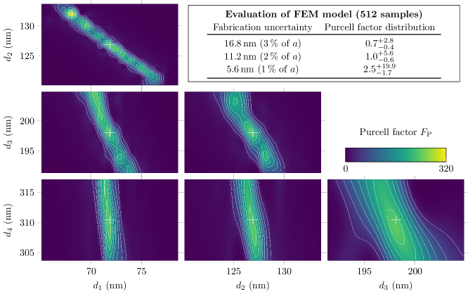
Figure 4: Following the initial sampling and optimization of the complete parameter space (as given in Table 1) an optimum $\bm{p}_{\mathrm{naive}}=\left[71.9,126.9,198.1,310.4\right]\,$\mathrm{nm}$$ was determined. This optimum is part of a very narrow ridge. When uncertainties in the manufacturing process are taken into consideration, the theoretically extremely high Purcell enhancements become difficult to achieve in reality. For example, assuming that the manufacturing process scatters according to a normal distribution with a standard deviation of $16.8\text{\,}\mathrm{nm}$ in each parameter, one can realistically expect a median Purcell enhancement of $\overline{F}_{\mathrm{P}}=0.7_{-0.4}^{+2.8}$, despite selecting a parameter that should theoretically reach values of $F_{\mathrm{P}}>200$.

4.3 Comparing to the naïve ansatz

The initial generation of training data $\bm{Y}_{\mathrm{train,first}}$ in the beginning of the first pass can be considered to be part of a conventional optimization procedure which seeks to maximize the Purcell enhancement of the photonic crystal nanobeam cavity in the parameter space Table 1. To complete this optimization, we took the largest function value in $\bm{Y}_{\mathrm{train,first}}$ and the associated parameter, and converged them using a Bayesian optimizer. The employed objective function was the FEM model $f(\bm{p})$, as such no optimization w.r.t. robustness took place. The BO method determined a parameter $\bm{p}_{\mathrm{naive}}=\left[71.9,126.9,198.1,310.4\right]\,$\mathrm{nm}$$ associated with a Purcell enhancement of $F_{\mathrm{P}}\approx$256.5$$.

We have calculated the expected Purcell enhancement of the found parameter $\bm{p}_{\mathrm{naive}}$ by applying the methodology described in Section 2.3, where $M_{\mathrm{device}}=$512$$ samples were used to evaluate the FEM model $f(\bm{p})$. We found that given a manufacturing uncertainty of $\sigma_{d_{i}}=$16.8\text{\,}\mathrm{nm}$$ that even despite the very high Purcell enhancement of $F_{\mathrm{P}}\approx$256.5$$, we can only expect to achieve a Purcell enhancement of $\overline{F}_{\mathrm{P}}=0.7_{-0.4}^{+2.8}$ when actually manufacturing the device. This value can be improved by reducing the manufacturing uncertainties. For a manufacturing uncertainty of $11.2\text{\,}\mathrm{nm}$, i.e., $2\text{\,}\mathrm{\char 37\relax}$ of the unit cell pitch $a$, we achieved $\overline{F}_{\mathrm{P}}=1.0_{-0.6}^{+5.6}$, and for a manufacturing uncertainty of $5.6\text{\,}\mathrm{nm}$,i.e., $1\text{\,}\mathrm{\char 37\relax}$ of the unit cell pitch $a$, we achieved $\overline{F}_{\mathrm{P}}=2.5_{-1.7}^{+19.9}$.

We have visualized the close surroundings of the found optimum $\bm{p}_{\mathrm{naive}}$ in Figure 4. Note that, in the creation of the figure, parameters with even higher Purcell enhancements ($F_{\mathrm{P}}>$300$$) were discovered. This highlights the challenges associated with optimizing the forward model function $f(\bm{p})$ in such a large parameter space, even in an unrobust fashion. The size of the shown parameter space is such that the $1\sigma$ ellipsis of a $5.6\text{\,}\mathrm{nm}$ manufacturing uncertainty would touch the borders of the sub figures. We observed that the found maximum is very narrow. Manufacturing a cavity that exploits this maximum thus requires very good control over the manufacturing uncertainties.

5 Summary

We have presented an approach for a robust design optimization that takes manufacturing uncertainties in the fabrication process into account. We have applied it to optimize the FEM model of a hole based photonic crystal nanobeam cavity such that we obtain a Purcell enhancement that is robust under an assumed manufacturing uncertainty of $\sigma_{d_{i}}=$16.8\text{\,}\mathrm{nm}$$ for each of the varied device parameters.

The approach is based on a Monte Carlo integration procedure that is accelerated by using trained Gaussian process surrogate models. These help to manage the high computational burden imposed by the employed finite element forward model function $f(\bm{p})$. The GP surrogates are adapted to deal with the bounded nature of the optimized Purcell enhancement. During the application, a transformation function is learned that maps the training data and the GPs predictions between the bounded domain of the training data and the unbounded domain of the GP predictions.

The presented approach itself is iterative. First, a coarse analysis is performed on a very large domain. The results of this coarse analysis are used to inform a finer analysis that focuses on a much smaller domain. During the coarse analysis, we found that a region centered around $\bm{p}_{\mathrm{opt,first}}=\left[428.6,282.5,369.5,253\right]\,$\mathrm{nm}$$ is predicted to have a robust Purcell enhancement of $\overline{F}_{\mathrm{P}}\approx$9.4$$ (based on the coarse GP surrogate). Evaluating the forward model function attested a robust Purcell enhancement of $\overline{F}_{\mathrm{P}}\approx$2.3$$. Considering the very coarse nature of the GP surrogate, we deemed this as a reasonable agreement, since large portions of the parameter space have small $F_{\mathrm{P}}$. During the fine analysis of the region centered around $\bm{p}_{\mathrm{opt,first}}$, we found that the parameter $\bm{p}_{\mathrm{robust}}=\left[412,311.5,392,250.3\right]\,$\mathrm{nm}$$ is robust against a manufacturing uncertainty of $\sigma_{d_{i}}=$16.8\text{\,}\mathrm{nm}$$, and is capable of reaching a robust Purcell enhancement of $\overline{F}_{\mathrm{P}}=(3.6\pm 1.1)_{-2.7}^{+6.6}$. The parameter was verified using the forward model function $f(\bm{p})$. Here, we found that $\overline{F}_{\mathrm{P}}=3.2_{-2.3}^{+8.6}$, which confirmed the predictions of the GP surrogate within the prediction uncertainty and is an improvement over the results of the first pass.

The result was compared to a naïve ansatz in which we directly optimized the forward model function $f(\bm{p})$, i.e., found a candidate $\bm{p}_{\mathrm{naive}}=\arg\max f(\bm{p})$ and then determined the robustness of the found parameter. Here, we found that, despite the fact that the $\bm{p}_{\mathrm{naive}}$ we found is associated with a Purcell enhancement of $F_{\mathrm{P}}\approx$256.5$$, we can only expect a robust Purcell enhancement of $\overline{F}_{\mathrm{P}}=0.7_{-0.4}^{+2.8}$ when taking manufacturing uncertainties into account. The reason for this is that $\bm{p}_{\mathrm{naive}}$ is situated in a very narrow ridge. In order to exploit the high Purcell enhancement tied to this ridge, the manufacturing uncertainties have to be controlled to a much tighter degree than assumed in this article.

We have therefore shown that our approach is capable of generating a result that is more than four times better than the naïve approach when manufacturing uncertainties play a role.

Data availability

The Python scripts for performing the robust design optimization, as well as the research data, are available on Zenodo in the data publication found under [61].

Appendix

A Variation of the fabrication uncertainties

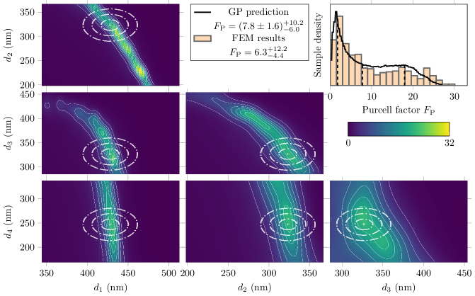
Figure A.1: The function value landscape around the robust design parameter $\bm{p}_{\mathrm{robust}}^{\prime}=\left[428.1,323.9,326,246.8\right]\,$\mathrm{nm}$$ (marked with a white cross). The white ellipses around the white cross indicate (from smallest to largest) the $1\sigma$, $2\sigma$, and $3\sigma$ percentiles of the manufacturing distribution, which was assumed to be a multivariate normal distribution. The covariance matrix of this multivariate normal distribution was chosen to be $\mathbf{\Sigma}_{\mathrm{manuf}}={\rm diag}(\sigma_{d}^{2},\sigma_{d}^{2},\sigma_{d}^{2},\sigma_{d}^{2})$ with $\sigma_{d}=$11.2\text{\,}\mathrm{nm}$$. Applying Algorithm 1 in conjunction with a trained surrogate model allowed us to efficiently determine that a manufacturing process that produces devices according to a normal distribution with $\mathcal{N}(\bm{p}_{\mathrm{robust}}^{\prime},\mathbf{\Sigma}_{\mathrm{manuf}})$ yields devices with an expected Purcell enhancement $\overline{F}_{\mathrm{{P}}}=(7.8\pm 1.6)_{-6.0}^{+10.2}$. Verification using the FEM model showed that $\overline{F}_{\mathrm{P}}=6.3_{-4.4}^{+12.2}$. Both results are shown in the top right sub figure.

It is computationally relatively cheap to consider different manufacturing uncertainties for an already trained surrogate model. We considered here the surrogate that was trained in the second pass Section 4.2.2, which was defined on the domain listed in Table 2. If we assume that we can reduce the manufacturing uncertainty to $11.2\text{\,}\mathrm{nm}$ for each of the $d_{i}$ (i.e., to $2\text{\,}\mathrm{\char 37\relax}$ of the unit cell pitch $a$), then a parameter $\bm{p}=\left[428.1,323.9,326,246.8\right]\,$\mathrm{nm}$$ would lead to a predicted robust Purcell enhancement of $\overline{F}_{\mathrm{P}}=(7.8\pm 1.6)_{-6.0}^{+10.2}$. The results were verified using FEM, with $\overline{F}_{\mathrm{P}}=6.3_{-4.4}^{+12.2}$. In either case the expected Purcell enhancement was approximately doubled. The results are shown in Figure A.1.

References

- [1] N. Wang, W. Yan, Y. Qu, S. Ma, S. Z. Li, and M. Qiu, “Intelligent designs in nanophotonics: from optimization towards inverse creation,” PhotoniX, vol. 2, no. 1, pp. 1–35, 2021.
- [2] J. S. Jensen and O. Sigmund, “Topology optimization for nano-photonics,” Laser Photonics Rev., vol. 5, no. 2, pp. 308–321, 2011.
- [3] R. E. Christiansen and O. Sigmund, “Inverse design in photonics by topology optimization: tutorial,” J. Opt. Soc. Am. B, vol. 38, no. 2, pp. 496–509, 2021.
- [4] S. Mao, L. Cheng, C. Zhao, F. N. Khan, Q. Li, and H. Fu, “Inverse design for silicon photonics: From iterative optimization algorithms to deep neural networks,” Appl. Sci., vol. 11, no. 9, p. 3822, 2021.
- [5] M. Plock, K. Andrle, S. Burger, and P.-I. Schneider, “Bayesian Target-Vector Optimization for Efficient Parameter Reconstruction,” Adv. Theor. Simul., vol. 5, no. 10, p. 2200112, 2022.
- [6] J. Pomplun, S. Burger, L. Zschiedrich, and F. Schmidt, “Adaptive finite element method for simulation of optical nano structures,” Phys. Status Solidi B, vol. 244, p. 3419, 2007.
- [7] A. Taflove, S. C. Hagness, and M. Piket-May, “Computational electromagnetics: the finite-difference time-domain method,” Electr. Eng. Handb., vol. 3, no. 629-670, p. 15, 2005.
- [8] M. A. Iqbal, N. Ashraf, W. Shahid, M. Awais, A. K. Durrani, K. Shahzad, and M. Ikram, “Nanophotonics: Fundamentals, Challenges, Future Prospects and Applied Applications,” in Nonlinear Opt. IntechOpen, 2021, ch. 2.
- [9] S. Molesky, Z. Lin, A. Y. Piggott, W. Jin, J. Vucković, and A. W. Rodriguez, “Inverse design in nanophotonics,” Nat. Photonics, vol. 12, no. 11, pp. 659–670, 2018.
- [10] T. Asano, Y. Ochi, Y. Takahashi, K. Kishimoto, and S. Noda, “Photonic crystal nanocavity with a Q factor exceeding eleven million,” Opt. Express, vol. 25, no. 3, pp. 1769–1777, 2017.
- [11] M. Minkov and V. Savona, “Automated optimization of photonic crystal slab cavities,” Sci. Rep., vol. 4, no. 1, p. 5124, 2014.
- [12] P. B. Deotare, M. W. McCutcheon, I. W. Frank, M. Khan, and M. Lončar, “High quality factor photonic crystal nanobeam cavities,” Appl. Phys. Lett., vol. 94, no. 12, 2009.
- [13] H. Hagino, Y. Takahashi, Y. Tanaka, T. Asano, and S. Noda, “Effects of fluctuation in air hole radii and positions on optical characteristics in photonic crystal heterostructure nanocavities,” Phys. Rev. B, vol. 79, p. 085112, 2009.
- [14] A. Oskooi, A. Mutapcic, S. Noda, J. D. Joannopoulos, S. P. Boyd, and S. G. Johnson, “Robust optimization of adiabatic tapers for coupling to slow-light photonic-crystal waveguides,” Opt. Express, vol. 20, no. 19, pp. 21 558–21 575, 2012.
- [15] D. O. Bracher and E. L. Hu, “Fabrication of high-Q nanobeam photonic crystals in epitaxially grown 4H-SiC,” Nano Lett., vol. 15, no. 9, pp. 6202–6207, 2015.
- [16] G.-J. Park, T.-H. Lee, K. H. Lee, and K.-H. Hwang, “Robust Design: An Overview,” AIAA J., vol. 44, no. 1, pp. 181–191, 2006.
- [17] H.-G. Beyer and B. Sendhoff, “Robust optimization – A comprehensive survey,” Comput. Methods Appl. Mech. Eng., vol. 196, no. 33, pp. 3190–3218, 2007.
- [18] A. Ben-Tal and A. Nemirovski, “Robust convex optimization,” Math. Oper. Res., vol. 23, no. 4, pp. 769–805, 1998.
- [19] V. Gabrel, C. Murat, and A. Thiele, “Recent advances in robust optimization: An overview,” Eur. J. Oper. Res., vol. 235, no. 3, pp. 471–483, 2014.
- [20] B. L. Gorissen, İ. Yanıkoğlu, and D. den Hertog, “A practical guide to robust optimization,” Omega, vol. 53, pp. 124–137, 2015.
- [21] A. Mutapcic, S. Boyd, A. Farjadpour, S. G. Johnson, and Y. Avniel, “Robust design of slow-light tapers in periodic waveguides,” Eng. Optim., vol. 41, no. 4, pp. 365–384, 2009.
- [22] T.-W. Weng, D. Melati, A. Melloni, and L. Daniel, “Stochastic simulation and robust design optimization of integrated photonic filters,” Nanophotonics, vol. 6, no. 1, pp. 299–308, 2017.
- [23] D. Gostimirovic, Y. Grinberg, D.-X. Xu, and O. Liboiron-Ladouceur, “Improving Fabrication Fidelity of Integrated Nanophotonic Devices Using Deep Learning,” ACS Photonics, 2023.
- [24] M. Pozzi, G. Bonaccorsi, H. A. Kim, and F. Braghin, “Robust structural optimization in presence of manufacturing uncertainties through a boundary-perturbation method,” Struct. Multidiscip. Optim., vol. 66, no. 6, pp. 1–13, 2023.
- [25] P. R. Wiecha, A. Arbouet, C. Girard, and O. L. Muskens, “Deep learning in nano-photonics: inverse design and beyond,” Photon. Res., vol. 9, no. 5, pp. B182–B200, 2021.
- [26] C. P. Robert, G. Casella, and G. Casella, Monte Carlo statistical methods, 2nd ed. Springer, 1999.
- [27] K. P. Murphy, Machine learning: a probabilistic perspective. MIT press, 2012.
- [28] P. Kall and S. W. Wallace, Stochastic programming, 2nd ed. Springer, 1994.
- [29] J. R. Birge and F. Louveaux, Introduction to stochastic programming. Springer Science & Business Media, 2011.
- [30] C. K. Williams and C. E. Rasmussen, Gaussian processes for machine learning. MIT press Cambridge, MA, 2006.
- [31] J. M. Bopp, M. Plock, T. Turan, G. Pieplow, S. Burger, and T. Schröder, “’Sawfish’Photonic Crystal Cavity for Near-Unity Emitter-to-Fiber Interfacing in Quantum Network Applications,” arXiv preprint arXiv:2210.04702, 2022.
- [32] R. Garnett, Bayesian Optimization. Cambridge University Press, 2023.
- [33] P.-I. Schneider, X. Garcia Santiago, V. Soltwisch, M. Hammerschmidt, S. Burger, and C. Rockstuhl, “Benchmarking five global optimization approaches for nano-optical shape optimization and parameter reconstruction,” ACS Photonics, vol. 6, no. 11, pp. 2726–2733, 2019.
- [34] L. Rickert, F. Betz, M. Plock, S. Burger, and T. Heindel, “High-performance designs for fiber-pigtailed quantum-light sources based on quantum dots in electrically-controlled circular Bragg gratings,” Opt. Express, vol. 31, no. 9, pp. 14 750–14 770, 2023.
- [35] J. Martin and T. Simpson, “A Monte Carlo Method for Reliability-Based Design Optimization,” in 47th AIAA/ASME/ASCE/AHS/ASC Structures, Structural Dynamics, and Materials Conference, 2006, p. 2146.
- [36] K.-H. Lee and G.-J. Park, “A global robust optimization using Kriging based approximation model,” JSME Int J., Ser. C, vol. 49, no. 3, pp. 779–788, 2006.
- [37] J. D. Joannopoulos, S. G. Johnson, J. N. Winn, and R. D. Meade, Photonic Crystals: Molding the Flow of Light. Princeton University Press, Princeton, NJ, 2008.
- [38] P. B. Deotare and M. Loncar, “Photonic crystal nanobeam cavities,” in Encyclopedia of Nanotechnology. Springer Netherlands, 2012, pp. 2060–2069.
- [39] E. M. Purcell, “Spontaneous emission probabilities at radio frequencies,” Phys. Rev., vol. 69, p. 681, 1946.
- [40] M. H. DeGroot and M. J. Schervish, Probability and statistics, 4th ed. Addison-Wesley, 2012.
- [41] E. Brochu, V. M. Cora, and N. De Freitas, “A tutorial on Bayesian optimization of expensive cost functions, with application to active user modeling and hierarchical reinforcement learning,” arXiv preprint arXiv:1012.2599, 2010.
- [42] G. Montavon, W. Samek, and K.-R. Müller, “Methods for interpreting and understanding deep neural networks,” Digital Signal Process., vol. 73, pp. 1–15, 2018.
- [43] C. E. Rasmussen, “Gaussian processes to speed up hybrid Monte Carlo for expensive Bayesian integrals,” in Seventh Valencia international meeting, dedicated to Dennis V. Lindley. Oxford University Press, 2003, pp. 651–659.
- [44] X. Garcia-Santiago, P.-I. Schneider, C. Rockstuhl, and S. Burger, “Shape design of a reflecting surface using Bayesian Optimization,” in J. Phys. Conf. Ser., vol. 963, no. 1. IOP Publishing, 2018, p. 012003.
- [45] E. Snelson, Z. Ghahramani, and C. Rasmussen, “Warped Gaussian Processes,” Adv. Neural Inf. Process., vol. 16, 2003.
- [46] M. Lázaro-Gredilla, “Bayesian warped Gaussian processes,” Adv. Neural Inf. Process., vol. 25, 2012.
- [47] D. R. Jones, M. Schonlau, and W. J. Welch, “Efficient global optimization of expensive black-box functions,” J. Global Optim., vol. 13, pp. 455–492, 1998.
- [48] T. Hastie, R. Tibshirani, J. H. Friedman, and J. H. Friedman, The elements of statistical learning: data mining, inference, and prediction. Springer, 2009, vol. 2.
- [49] F. Sun, Z. Li, B. Tang, B. Li, P. Zhang, R. Liu, G. Yang, K. Huang, Z. Han, J. Luo, W. Wang, and Y. Yang, “Scalable high Q-factor Fano resonance from air-mode photonic crystal nanobeam cavity,” Nanophotonics, vol. 12, no. 15, pp. 3135–3148, 2023.
- [50] T. Weise, M. Zapf, R. Chiong, and A. J. Nebro, Nature-Inspired Algorithms for Optimisation. Berlin, Heidelberg: Springer Berlin Heidelberg, 2009, ch. Why Is Optimization Difficult?, pp. 1–50.
- [51] F. Y. Kuo and I. H. Sloan, “Lifting the curse of dimensionality,” Not. Am. Math. Soc., vol. 52, no. 11, pp. 1320–1328, 2005.
- [52] I. M. Sobol’, “On the distribution of points in a cube and the approximate evaluation of integrals,” Zh. Vychisl. Mat. Mat. Fiz., vol. 7, no. 4, pp. 784–802, 1967.
- [53] S. Joe and F. Y. Kuo, “Constructing Sobol sequences with better two-dimensional projections,” SIAM J. Sci. Comput., vol. 30, no. 5, pp. 2635–2654, 2008.
- [54] A. B. Owen, “On dropping the first Sobol’ point,” in International conference on Monte Carlo and quasi-Monte Carlo methods in scientific computing. Springer, 2020, pp. 71–86.
- [55] R. H. Byrd, P. Lu, J. Nocedal, and C. Zhu, “A limited memory algorithm for bound constrained optimization,” SIAM J. Sci. Comput., vol. 16, no. 5, pp. 1190–1208, 1995.
- [56] T. Dick, E. Wong, and C. Dann, “How many random restarts are enough,” Tech. rep., Carnegie Mellon University, Tech. Rep., 2014.
- [57] P. Lalanne, W. Yan, K. Vynck, C. Sauvan, and J.-P. Hugonin, “Light Interaction with Photonic and Plasmonic Resonances,” Laser Photonics Rev., vol. 12, p. 1700113, 2018.
- [58] P. T. Kristensen, K. Herrmann, F. Intravaia, and K. Busch, “Modeling electromagnetic resonators using quasinormal modes,” Adv. Opt. Photon., vol. 12, no. 3, p. 612, 2020.
- [59] C. Sauvan, J.-P. Hugonin, I. S. Maksymov, and P. Lalanne, “Theory of the Spontaneous Optical Emission of Nanosize Photonic and Plasmon Resonators,” Phys. Rev. Lett., vol. 110, p. 237401, 2013.
- [60] T. Müller, J. Skiba-Szymanska, A. Krysa, J. Huwer, M. Felle, M. Anderson, R. Stevenson, J. Heffernan, D. A. Ritchie, and A. Shields, “A quantum light-emitting diode for the standard telecom window around 1,550 nm,” Nat. Commun., vol. 9, no. 1, p. 862, 2018.
- [61] M. Plock, F. Binkowski, L. Zschiedrich, P.-I. Schneider, and S. Burger, “Research data for the paper ”Fabrication uncertainty aware and robust design optimization of a photonic crystal nanobeam cavity by using Gaussian processes”,” on Zenodo, 2023. [Online]. Available: https://doi.org/10.5281/zenodo.8131611