The number of global solutions for GPS source localization in two-dimension

Abstract

Source localization is widely used in many areas including GPS, but the influence of possible noises is not so negligible. Many optimization methods are attempted to alleviate different kinds of noises. Needless to say the stability of the solution, even the number of global solutions are not fully known. Only local convergence or stability for the optimization problem are known in simple $L^{1}$[2] or $L^{2}$[3] settings. In this paper, we prove that the number of possible two dimensional source locations with three measurements in $L^{2}$ setting, is at most $5$, which is the complement and correction to the previous work [3]. We also showed the sufficient and necessary condition for the number of the solutions being 1,2,3,4,and 5, where the measurement triangle is isosceles and the measurement distance for the two isosceles triangle bases are the same.

1 Introduction

Let $Z_{1},Z_{2},Z_{3}\in\mathbb{R}^{2}$ be the sensor locations and $X\in\mathbb{R}^{2}$ be the possible source position. Denote $d_{i},i=1,2,3$ as the measurement length between the $i$-th sensor and the source having noise $\epsilon_{i}$:

$$d_{i}=||X-Z_{i}||+\epsilon_{i}.$$ (1)

Let $Z=(Z_{1},Z_{2},Z_{3})\in(\mathbb{R}^{2})^{3}$, $d=(d_{1},d_{2},d_{3})\in\mathbb{R}^{3},\epsilon=(\epsilon_{1},\epsilon_{2},\epsilon_{3})\in\mathbb{R}^{3}$, and $X$ be the solutions of the following minimization problem:

$$X=\mathrm{argmin}_{W\in\mathbb{R}^{2}}O(W),\mbox{ where }O(W)=\sum_{j=1}^{3}|||W-Z_{j}||^{2}-d_{j}^{2}|$$ (2)

By Proposition 1 [2], there exists at least one solution $X$. If we notate $|X|$ as the number of possible locations set $X$, then $|X|\geq 1$.

Let $S_{1},S_{2},$ and $S_{3}$ be the measurement circles, and further define

$$S=S_{1}\cup S_{2}\cup S_{3},\;\;S_{123}=S_{12}\cup S_{23}\cup S_{31},\;\;S_{23}=S_{2}\cap S_{3},\;S_{31}=S_{3}\cap S_{1},\;S_{12}=S_{1}\cap S_{2}.$$

By definition, $S_{ij}=S_{ji}$. Assuming $|S_{12}|=2$, let $S_{12+}$ and $S_{12-}$ be the points having shortest and longest distances from $Z_{3}$ in $S_{12}$, respectively. If $|S_{12}|=1$, define $S_{12+}=S_{12-}=S_{12}$. We can also define $S_{23+},S_{23-},S_{31+},$ and $S_{31-}$ in the same way. Denote $S_{123+}=\{S_{12+},S_{23+},S_{31+}\}$ and $S_{123-}=\{S_{12-},S_{23-},S_{31-}\}$.

Let $R_{i_{1},i_{2},i_{3}}$ be the intersection of closed disks with $i_{l}=1$ and the outside of open disks with $i_{l}=0$ for $l=1,2,$ and $3$. That is to say, $R_{i_{1},i_{2},i_{3}}$ is a closed set. Let

$$R_{l}=\cup_{i_{1}+i_{2}+i_{3}=l}R_{i_{1},i_{2},i_{3}},$$

then we have

$$\mathbb{R}^{2}=R_{0}\cup R_{1}\cup R_{2}\cup R_{3}.$$

The number of possible source locations to (2) is already explained in [2]. But Theorem 2(a), 2(b), and 6(c) in [2] are misleading. Therefore, we correct the theorems in Theorem 1 and 2, where red phrases are the corrected ones to the thorems of [2]. Thus, Table 1 in [2] should be changed into Table 1 in the present paper.

	[3], the present work	[2]
The objective function	$O(W)=\sum_{j=1}^{3}|d_{j}^{2}-||W-Z_{j}||^{2}|$	$O(W)=\sum_{j=1}^{3}|d_{j}-||W-Z_{j}|||$
Existence	Holds	Holds
$|X|$	$1,2,3{\color[rgb]{1,0,0},4,\mbox{ and }5}$	$1,2,\cdots,\infty$
$|X|=1$ for nonempty $K$	Holds	Holds when $K$ is connected
Uniqueness when $K$ is empty	Holds when $R_{3}=\phi$ or one of	Does not hold
	$R_{100},R_{010},$ and $R_{001}$ is empty or not connected.
Nonuniqueness examples	Shown for all cases with $|X|=2,3{\color[rgb]{1,0,0},4,\mbox{ and }5}$	Shown for $|X|=2,3$
		and not shown for $|X|=4,5,\cdots$
Detailed position	Given only when $K$ is nonempty	Given only when $K$ is nonempty
	or when $|Z_{3}Z_{1}|=|Z_{3}Z_{2}|$ and $d_{1}=d_{2}$

Table 1: Differences among the results in [2],[3], and the present work. $K=R_{0}\cap\triangle Z_{1}Z_{2}Z_{3}$.

Theorem 3 shows that the number of solutions can be $|X|=2,4,$ and $5$, where only the cases with $|X|=1,2,$ and $3$ are shown in [2].

Theorem 1.

The condition $|X|=2,3,{\color[rgb]{1,0,0}4,\mbox{ and }5}$ holds if and only if $R_{3}\neq\phi$ and $R_{100},R_{010},$ and $R_{001}$ are connected and nonempty, respectively. If one of these conditions holds, we have $X=argmin_{A\in{\color[rgb]{1,0,0}S_{123}^{\pm}}}\left\lVert A-Y_{0}\right\rVert$.

From Theorem 1, we have $|X|\leq 6$. Thus, the following theorem holds if we prove $|X|\neq 6$:

Theorem 2.

There are at most five solutions.

Theorem 3.

Suppose that

$$\left\lVert Z_{1}Z_{3}\right\rVert=\left\lVert Z_{2}Z_{3}\right\rVert,\;d_{1}=d_{2}>\left\lVert Z_{1}Z_{3}\right\rVert,\;d_{3}^{2}=d_{1}^{2}-\left\lVert Z_{1}Z_{3}\right\rVert^{2}.$$

Let us denote

$$P=\sqrt{\frac{\left\lVert Z_{1}Z_{2}\right\rVert^{2}}{4}+\left(\left\lVert Z_{1}Z_{3}\right\rVert^{2}-\frac{\left\lVert Z_{1}Z_{2}\right\rVert^{2}}{4}\right)\left(\frac{\left\lVert Z_{1}Z_{3}\right\rVert^{2}+\left\lVert Z_{1}Z_{2}\right\rVert^{2}}{\left\lVert Z_{1}Z_{3}\right\rVert^{2}-\left\lVert Z_{1}Z_{2}\right\rVert^{2}}\right)^{2}},$$

only when $\left\lVert Z_{1}Z_{3}\right\rVert>\left\lVert Z_{1}Z_{2}\right\rVert$. Depending on $d_{1}$ and $\frac{\left\lVert Z_{1}Z_{3}\right\rVert}{\left\lVert Z_{1}Z_{2}\right\rVert}$, we have the minimum $X$ as follows:

$$\begin{array}[]{cc}\mbox{If }\left\lVert Z_{1}Z_{3}\right\rVert\leq\left\lVert Z_{1}Z_{2}\right\rVert\mbox{ or }d_{1}<P,&\mbox{then }X=\{S_{12+}\}\\ \mbox{If }\left\lVert Z_{1}Z_{3}\right\rVert>\left\lVert Z_{1}Z_{2}\right\rVert\mbox{ and }d_{1}=P,&\mbox{then }X=\{S_{12+},S_{23\pm},S_{31\pm}\}\\ \mbox{If }\left\lVert Z_{1}Z_{3}\right\rVert>\left\lVert Z_{1}Z_{2}\right\rVert\mbox{ and }d_{1}>P,&\mbox{then }X=\{S_{23\pm},S_{31\pm}\}\end{array}$$

The number of solutions when the measurement triangle and three measurements satisfy the assumption of Theorem 3, is displayed in Fig. 1 depending on $\frac{\left\lVert Z_{1}Z_{2}\right\rVert}{\left\lVert Z_{1}Z_{3}\right\rVert}$ and $d_{1}$ (with respect to $P$) and the object values at the intersections of measurement circles are displayed in Table 2.

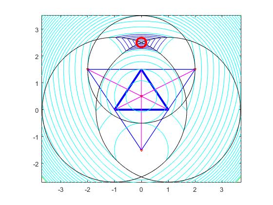
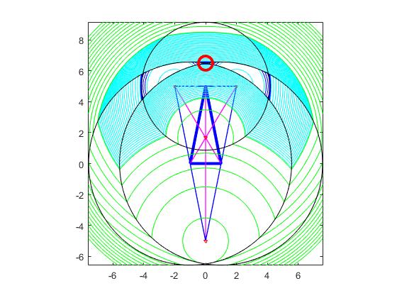
(a)                    (b)

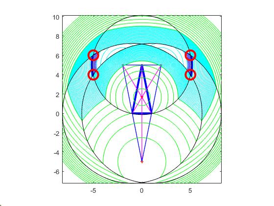
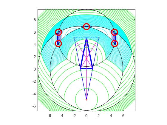
(c)                    (d)

Figure 1: The figure for Theorem 3 when $\left\lVert Z_{1}Z_{2}\right\rVert=2$. The solutions are (a) $X=\{S_{12+}\}$ when $\left\lVert Z_{1}Z_{3}\right\rVert<\left\lVert Z_{1}Z_{2}\right\rVert$, (b) $X=\{S_{12+}\}$ when $\left\lVert Z_{1}Z_{3}\right\rVert<\left\lVert Z_{1}Z_{2}\right\rVert$ and $d_{1}<P$, (c) $X=\{S_{23\pm},S_{31\pm}\}$ when $\left\lVert Z_{1}Z_{3}\right\rVert<\left\lVert Z_{1}Z_{2}\right\rVert$ and $d_{1}>P$, and (d) $X=\{S_{12+},S_{23\pm},S_{31\pm}\}$ when $\left\lVert Z_{1}Z_{3}\right\rVert<\left\lVert Z_{1}Z_{2}\right\rVert$ and $d_{1}=P$ .

	$O(S_{12+})$	$O(S_{23+})$	$O(S_{31+})$	$O(S_{12-})$	$O(S_{23-})$	$O(S_{31-})$
Fig. 1 (a)	3.0000	6.6564	6.6564	12.0000	6.6564	6.6564
Fig. 1 (b)	14.8862	16.2207	16.2207	114.8862	16.2207	16.2207
Fig. 1 (c)	21.6750	20.1430	20.1430	121.6750	20.1430	20.1430
Fig. 1 (d)	18.1818	18.1818	18.1818	118.1818	18.1818	18.1818

Table 2: The comparison of objective values at $S_{12\pm},S_{23\pm},$ and $S_{31\pm}$ for Fig. 1.

From the Theorem 3, we can derive the equivalent condition for $|X|=5$ as follows:

Corollary 4.

$|X|=5$ if and only if

$$\left\lVert Z_{1}Z_{3}\right\rVert=\left\lVert Z_{2}Z_{3}\right\rVert,\;\left\lVert Z_{1}Z_{3}\right\rVert>\left\lVert Z_{1}Z_{2}\right\rVert,\;d_{1}^{2}=\frac{\left\lVert Z_{1}Z_{2}\right\rVert^{2}}{4}+\left(\left\lVert Z_{1}Z_{3}\right\rVert^{2}-\frac{\left\lVert Z_{1}Z_{2}\right\rVert^{2}}{4}\right)\left(\frac{\left\lVert Z_{1}Z_{3}\right\rVert^{2}+\left\lVert Z_{1}Z_{2}\right\rVert^{2}}{\left\lVert Z_{1}Z_{3}\right\rVert^{2}-\left\lVert Z_{1}Z_{2}\right\rVert^{2}}\right)^{2},$$

$$d_{3}=\sqrt{d_{1}^{2}-\left\lVert Z_{1}Z_{3}\right\rVert^{2}},\;d_{2}=d_{1}.$$

by reordering if necessary.

In Section 3, we will prove Theorem 1, 2, and 3. The lemmas for the proof of the theorems are stated and proved in Section 2. The number and exact locations of the solutions are presented in Section 4 and 5, when the measurment triangle is equilateral and isosceles, respectively. Numerical results with Matlab ‘contour’ function are displayed with our suggested solutions. Tables 2, 3, and 4 for the objective values of $S_{12\pm},S_{23\pm},$ and $S_{31\pm}$,show that the suggested number of solutions are correct.

2 Lemmas

Denote $S_{ij0}:=\frac{S_{ij-}+S_{ij+}}{2}$ if $S_{i}$ and $S_{j}$ meet for $i,j=1,2,3,i\neq j$. We will notate ‘iff’ as an abbreviation of ‘if and only if’.

Lemma 5.

Assume that $S_{1}\cap S_{2}\neq\phi$. If

$$d_{3}^{0}:=\sqrt{\frac{1}{2}\left\lVert Z_{3}-S_{12+}\right\rVert^{2}+\frac{1}{2}\left\lVert Z_{3}-S_{12-}\right\rVert^{2}},$$

then we have

$$\left\{\begin{array}[]{ccc}O(S_{12+})<O(S_{12-})&\mbox{ iff }&d_{3}<d_{3,0},\\ O(S_{12+})=O(S_{12-})&\mbox{ iff }&d_{3}=d_{3,0},\\ O(S_{12+})>O(S_{12-})&\mbox{ iff }&d_{3}>d_{3,0}.\end{array}\right.$$ (3)

Proof.

Since $O(S_{12+})=\left|d_{3}^{2}-\left\lVert Z_{3}-S_{12+}\right\rVert^{2}\right|,\;O(S_{12-})=\left|d_{3}^{2}-\left\lVert Z_{3}-S_{12-}\right\rVert^{2}\right|,$ and $\left\lVert Z_{3}-S_{12+}\right\rVert\leq\left\lVert Z_{3}-S_{12-}\right\rVert$, we have (3). ∎

Let us define $d_{1,0}$ and $d_{2,0}$ likewise as in Lemma 5.

Lemma 6.

Suppose that $\left\lVert Z_{1}Z_{3}\right\rVert=\left\lVert Z_{2}Z_{3}\right\rVert$, $d_{1}=d_{2}$, and $R_{i_{1},i_{2},i_{3}}$ is nonempty and connected for all $i_{1},i_{2},i_{3}\in\{0,1\}$. Then, $O(S_{23+})=O(S_{31+}),\;O(S_{23+})=O(S_{23-})$, and we have

$$d_{3}^{0}=\sqrt{d_{1}^{2}+\left\lVert Z_{1}Z_{3}\right\rVert^{2}-\frac{\left\lVert Z_{1}Z_{2}\right\rVert^{2}}{2}}$$

and

$$d_{1}^{0}=d_{2}^{0}=\sqrt{d_{1}^{2}+(\left\lVert Z_{1}Z_{3}\right\rVert^{2}+d_{3}^{2}-d_{1}^{2})\frac{\left\lVert Z_{1}Z_{2}\right\rVert^{2}}{2\left\lVert Z_{1}Z_{3}\right\rVert^{2}}}.$$

Further, we have

$$\begin{array}[]{ccc}O(S_{23+})<O(S_{23-})&{\mbox{i}ff}&\left\lVert Z_{1}Z_{3}\right\rVert^{2}+d_{3}^{2}>d_{1}^{2},\\ O(S_{23+})=O(S_{23-})&{\mbox{i}ff}&\left\lVert Z_{1}Z_{3}\right\rVert^{2}+d_{3}^{2}=d_{1}^{2},\\ O(S_{23+})>O(S_{23-})&{\mbox{i}ff}&\left\lVert Z_{1}Z_{3}\right\rVert^{2}+d_{3}^{2}<d_{1}^{2}.\end{array}$$

Proof.

By the assumption, we have $S_{120}=\frac{Z_{1}+Z_{2}}{2}$ and $\left\lVert Z_{3}-S_{12\pm}\right\rVert=\left\lVert Z_{3}-S_{120}\right\rVert\mp\left\lVert S_{120}-S_{12+}\right\rVert$. Thus, we have

$$d_{3}^{0}=\sqrt{\left\lVert Z_{3}-S_{120}\right\rVert^{2}+\left\lVert S_{12+}-S_{120}\right\rVert^{2}}=\sqrt{d_{1}^{2}+\left\lVert Z_{1}Z_{3}\right\rVert^{2}-\frac{\left\lVert Z_{1}Z_{2}\right\rVert^{2}}{2}}.$$

Let us compute $d_{1}^{0}$. Since the line $\overleftrightarrow{Z_{2}Z_{3}}$ orthogonally bisects $\overline{S_{12+}S_{12-}}$ at $S_{230}$, we have $\angle S_{23+}Z_{3}Z_{2}=\angle S_{23-}Z_{3}Z_{2}$.

$$(d_{1}^{0})^{2} = \frac{1}{2}\left\lVert Z_{1}-S_{31+}\right\rVert^{2}+\frac{1}{2}\left\lVert Z_{1}-S_{23-}\right\rVert^{2}$$

$$= \frac{1}{2}d_{3}^{2}+\frac{1}{2}\left\lVert Z_{1}Z_{3}\right\rVert^{2}-d_{3}\left\lVert Z_{1}Z_{3}\right\rVert\cos(\angle Z_{1}Z_{3}Z_{2}+\angle Z_{2}Z_{3}S_{23-})$$

$$\frac{1}{2}d_{3}^{2}+\frac{1}{2}\left\lVert Z_{1}Z_{3}\right\rVert^{2}-d_{3}\left\lVert Z_{1}Z_{3}\right\rVert\cos(\angle Z_{1}Z_{3}Z_{2}-\angle Z_{2}Z_{3}S_{23+})$$

$$= d_{3}^{2}+\left\lVert Z_{3}Z_{2}\right\rVert^{2}-2d_{3}\left\lVert Z_{1}Z_{3}\right\rVert\cos(\angle Z_{1}Z_{3}Z_{2})\cos(\angle Z_{2}Z_{3}S_{23+})$$

$$= d_{3}^{2}+\left\lVert Z_{3}Z_{2}\right\rVert^{2}-2d_{3}\left\lVert Z_{1}Z_{3}\right\rVert\left(1-\frac{\left\lVert Z_{1}Z_{2}\right\rVert^{2}}{2\left\lVert Z_{3}Z_{1}\right\rVert^{2}}\right)\frac{d_{3}^{2}+\left\lVert Z_{3}Z_{1}\right\rVert^{2}-d_{1}^{2}}{2d_{3}\left\lVert Z_{3}Z_{1}\right\rVert}$$

$$= d_{1}^{2}+\frac{\left\lVert Z_{1}Z_{2}\right\rVert^{2}}{2\left\lVert Z_{3}Z_{1}\right\rVert^{2}}(d_{3}^{2}+\left\lVert Z_{3}Z_{1}\right\rVert^{2}-d_{1}^{2}).$$

Hence, $d_{1}<d_{1}^{0}$ iff $d_{1}^{2}<d_{3}^{2}+\left\lVert Z_{3}Z_{1}\right\rVert^{2}$ and we proved the lemma. ∎

Further, let us define $Y_{0}:=\frac{1}{3}\sum_{i}Z_{i}$ and $Y_{j}=3Y_{0}-2Z_{j}$ for $j=1,2,3$.

Lemma 7.

Suppose that $S_{23-},S_{31-}\in R_{0}$. Then, $O(S_{23-})=O(S_{31-})$ iff

$$\left\lVert S_{23-}-Y_{0}\right\rVert=\left\lVert S_{31-}-Y_{0}\right\rVert,\mbox{ and }\angle Z_{3}Y_{0}S_{23-}=\angle Z_{3}Y_{0}S_{31-}.$$

Suppose that $S_{12-},S_{23-},S_{31-}\in R_{0}$. Then, $O(S_{23-})=O(S_{31-})=O(S_{12-})$ iff

$$\left\lVert S_{23-}-Y_{0}\right\rVert=\left\lVert S_{31-}-Y_{0}\right\rVert=\left\lVert S_{12-}-Y_{0}\right\rVert,$$

and

$${}\angle Z_{3}Y_{0}S_{23-}&=\angle Z_{3}Y_{0}S_{31-}=\pi-\angle Z_{1}Y_{0}Z_{2},\\ {}\angle Z_{1}Y_{0}S_{31-}=\angle Z_{1}Y_{0}S_{12-}=\pi-\angle Z_{2}Y_{0}Z_{3},\\ {}\angle Z_{2}Y_{0}S_{12-}=\angle Z_{2}Y_{0}S_{23-}=\pi-\angle Z_{3}Y_{0}Z_{1}.$$ (4)

Proof.

Suppose that $S_{23-},S_{31-}\in R_{0}$. From the condition that $O(S_{23-})=O(S_{31-})$, we have $\left\lVert Z_{3}-S_{31-}\right\rVert=\left\lVert Z_{3}-S_{23-}\right\rVert$. If $W\in R_{0}$, we have

$$O(W)&=\left\lVert W-Z_{1}\right\rVert^{2}-d_{1}^{2}+\left\lVert W-Z_{2}\right\rVert^{2}-d_{2}^{2}+\left\lVert W-Z_{3}\right\rVert^{2}-d_{3}^{2}\\ =3\left\lVert W-Y_{0}\right\rVert^{2}-3\left\lVert Y_{0}\right\rVert^{2}-d_{1}^{2}-d_{2}^{2}-d_{3}^{2}+\left\lVert Z_{1}\right\rVert^{2}+\left\lVert Z_{2}\right\rVert^{2}+\left\lVert Z_{3}\right\rVert^{2}.$$ (5)

Since $S_{23-},S_{31-}\in R_{0}$, we have $\left\lVert S_{23-}-Y_{0}\right\rVert=\left\lVert S_{31-}-Y_{0}\right\rVert$. From $\left\lVert Z_{3}-S_{31-}\right\rVert=\left\lVert Z_{3}-S_{23-}\right\rVert$ and $\left\lVert S_{23-}-Y_{0}\right\rVert=\left\lVert S_{31-}-Y_{0}\right\rVert$, we have

$$\angle Z_{3}Y_{0}S_{23-}=\angle Z_{3}Y_{0}S_{31-},$$

as in Fig. 2 (a). The converse can be proved easily.

Suppose that $S_{12-},S_{23-},S_{31-}\in R_{0}$. From the condition that $O(S_{23-})=O(S_{31-})=O(S_{12-})$, we have $\left\lVert Z_{3}-S_{23-}\right\rVert=\left\lVert Z_{3}-S_{31-}\right\rVert,\left\lVert Z_{1}-S_{31-}\right\rVert=\left\lVert Z_{1}-S_{12-}\right\rVert,$ and $\left\lVert Z_{2}-S_{12-}\right\rVert=\left\lVert Z_{2}-S_{23-}\right\rVert.$ Since $S_{12-},S_{23-},S_{31-}\in R_{0}$, with the similar argument as above, we have

$$\left\lVert S_{23-}-Y_{0}\right\rVert=\left\lVert S_{31-}-Y_{0}\right\rVert=\left\lVert S_{12-}-Y_{0}\right\rVert.$$

And further with similar argument, we have

$$\angle Z_{3}Y_{0}S_{23-}=\angle Z_{3}Y_{0}S_{31-},\quad\angle Z_{1}Y_{0}S_{31-}=\angle Z_{1}Y_{0}S_{12-},\quad\angle Z_{2}Y_{0}S_{12-}=\angle Z_{2}Y_{0}S_{23-}.$$

Since $2(\angle Z_{3}Y_{0}S_{23-}+\angle Z_{1}Y_{0}S_{31-}+\angle Z_{2}Y_{0}S_{12-})=2\pi$, we have

$$\angle Z_{3}Y_{0}S_{23-}=\pi-(\angle Z_{1}Y_{0}S_{31-}+\angle Z_{2}Y_{0}S_{12-})=\pi-(\angle Z_{1}Y_{0}S_{12-}+\angle Z_{2}Y_{0}S_{12-})=\pi-\angle Z_{1}Y_{0}Z_{2}.$$

The two equations (LABEL:eq:-Angle2) and (LABEL:eq:-Angle3) can be derived similarly. The converse can be proved without difficulty. ∎

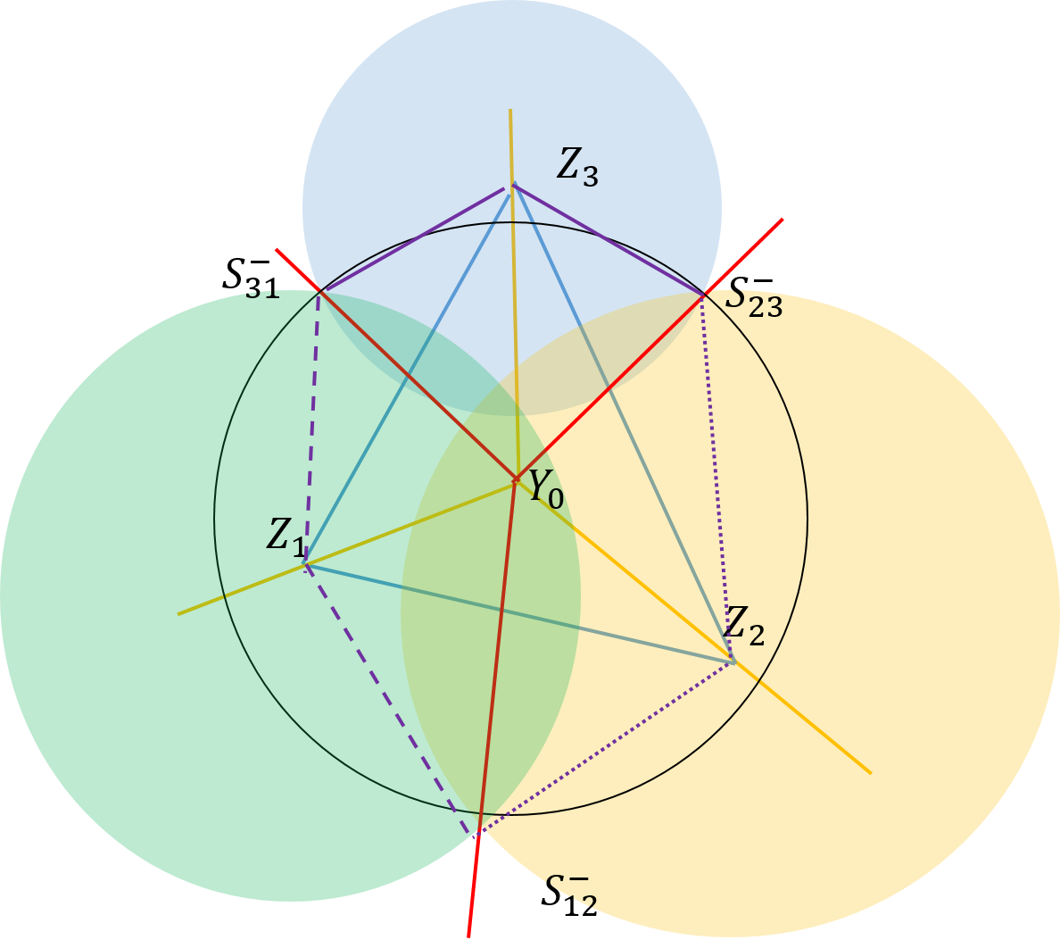
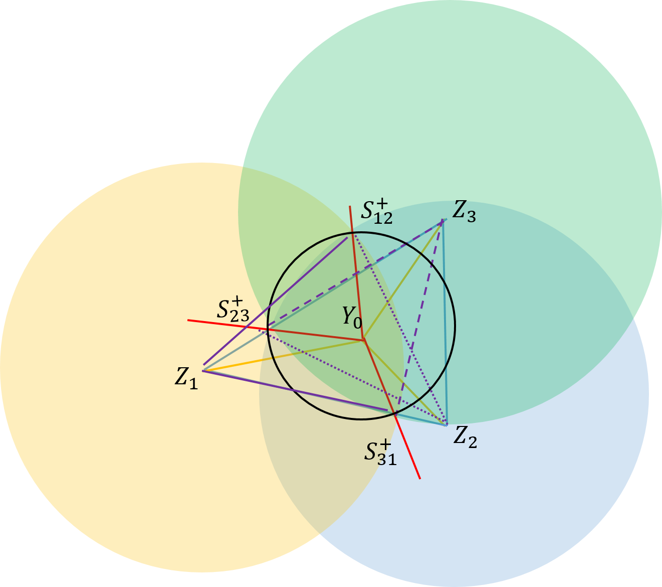
(a)                    (b)

Figure 2: The figure for (a) Lemma 7 and (b) Lemma 8.

Lemma 8.

If $S_{23+},S_{31+}\in R_{3}$ and $O(S_{23+})=O(S_{31+})$, then

$$\left\lVert S_{23+}-Y_{0}\right\rVert=\left\lVert S_{31+}-Y_{0}\right\rVert,$$

and

$$\angle Z_{3}Y_{0}S_{23+}=\angle Z_{3}Y_{0}S_{31+}.$$

If $S_{12+},S_{23+},S_{31+}\in R_{3}$ and $O(S_{23+})=O(S_{31+})=O(S_{12+})$, then

$$\left\lVert S_{23+}-Y_{0}\right\rVert=\left\lVert S_{31+}-Y_{0}\right\rVert=\left\lVert S_{12+}-Y_{0}\right\rVert,$$

and

$${}\angle Z_{3}Y_{0}S_{23+}&=\angle Z_{3}Y_{0}S_{31+}=\angle Z_{1}Y_{0}Z_{2},\\ {}\angle Z_{1}Y_{0}S_{31+}=\angle Z_{1}Y_{0}S_{12+}=\angle Z_{2}Y_{0}Z_{3},\\ {}\angle Z_{2}Y_{0}S_{12+}=\angle Z_{2}Y_{0}S_{23+}=\angle Z_{2}Y_{0}Z_{3}.$$ (6)

Proof.

We can prove the Lemma 8 with the same arguement as in Lemma 7. The only difference is the last equality in (6). We have the following equations when $O(S_{23+})=O(S_{31+})=O(S_{12+})$:

$$\angle Z_{3}Y_{0}S_{23+}=\angle Z_{3}Y_{0}S_{31+},\;\angle Z_{1}Y_{0}S_{31+}=\angle Z_{1}Y_{0}S_{12+},\;\angle Z_{2}Y_{0}S_{12+}=\angle Z_{2}Y_{0}S_{23+}.$$

And we can derive the followings (see Fig. 2 (b)) :

$$\angle Z_{1}Y_{0}S_{12+}+\angle Z_{2}Y_{0}S_{12+} = \angle Z_{1}Y_{0}Z_{3}+\angle Z_{2}Y_{0}Z_{3},$$

$$\angle Z_{2}Y_{0}S_{23+}+\angle Z_{3}Y_{0}S_{23+} = \angle Z_{3}Y_{0}Z_{1}+\angle Z_{2}Y_{0}Z_{1},$$

$$\angle Z_{3}Y_{0}S_{31+}+\angle Z_{1}Y_{0}S_{31+} = \angle Z_{3}Y_{0}Z_{2}+\angle Z_{1}Y_{0}Z_{2}.$$

Hence we have $\angle Z_{1}Y_{0}S_{12+}+\angle Z_{2}Y_{0}S_{23+}+\angle Z_{3}Y_{0}S_{31+}=\angle Z_{1}Y_{0}Z_{2}+\angle Z_{2}Y_{0}Z_{3}+\angle Z_{3}Y_{0}Z_{1}=2\pi$. From these equalities, we can derive the following:

$$\angle Z_{3}Y_{0}S_{23+}=2\pi-\left(\angle Z_{1}Y_{0}S_{31+}+\angle Z_{2}Y_{0}S_{12+}\right)=\angle Z_{1}Y_{0}S_{12+}+\angle Z_{2}Y_{0}S_{31+}=\angle Z_{1}Y_{0}S_{31+}+\angle Z_{2}Y_{0}S_{31+}=\angle Z_{1}Y_{0}Z_{2}.$$

The other two equalites (LABEL:eq:2D+1) and (LABEL:eq:2D+1) can be derived similarly. ∎

Let us notate $L=\frac{Z_{1}+Z_{2}}{2},M=\frac{Z_{2}+Z_{3}}{2},$ and $N=\frac{Z_{3}+Z_{1}}{2}$.

Lemma 9.

The condition that $R_{i1,i2,i3}$ is nonempty and connected for all $i_{1},i_{2}\in\{0,1\}$ and

$$O(S_{23+})=O(S_{23-})=O(S_{31+})=(S_{31-})$$

is equivalent to the following condition

$$\left\lVert Z_{1}Z_{3}\right\rVert=\left\lVert Z_{2}Z_{3}\right\rVert,d_{1}=d_{2},\mbox{ and }d_{1}^{2}=d_{3}^{2}+\left\lVert Z_{1}Z_{3}\right\rVert^{2}.$$

Proof.

Assume that $R_{i1,i2,i3}$ is nonempty and connected for all $i_{1},i_{2}\in\{0,1\}$ and

$$O(S_{23+})=O(S_{23-})=O(S_{31+})=(S_{31-}).$$

Possible locations of $S_{31+}$ and $S_{23+}$ are in Figure 3 (a) and (b). By using Lemma 7 and Lemma 8, we have

$$\angle Y_{0}Z_{3}S_{31+}=\angle Y_{0}Z_{3}S_{23+},\mbox{ and }\angle S_{31-}Z_{3}Y_{0}=\angle S_{23-}Z_{3}Y_{0}.$$

From these facts, we have

$$\angle Z_{1}Z_{3}Y_{0}=\angle Z_{2}Z_{3}Y_{0}.$$ (7)

From (7) and $\left\lVert Z_{1}L\right\rVert=\left\lVert Z_{2}L\right\rVert$, we have $\left\lVert Z_{1}Z_{3}\right\rVert=\left\lVert Z_{2}Z_{3}\right\rVert$ by the angle bisector theorem. Since

$$\angle Z_{1}S_{31-}Z_{3}=\frac{1}{2}\angle Z_{1}Z_{3}Y_{0}=\frac{1}{2}\angle Z_{2}Z_{3}Y_{0}=\angle Z_{2}S_{31-}Z_{3},$$

$\triangle Z_{1}S_{31-}Z_{3}$ and $\triangle Z_{2}S_{23-}Z_{3}$ are congruent and we can derive that $d_{1}=d_{2}$. By Lemma 6, we have $d_{1}^{2}=d_{3}^{2}+\left\lVert Z_{3}Z_{1}\right\rVert^{2}$.

From the condition $\left\lVert Z_{1}Z_{3}\right\rVert=\left\lVert Z_{2}Z_{3}\right\rVert,d_{1}=d_{2},\mbox{ and }d_{1}^{2}=d_{3}^{2}+\left\lVert Z_{1}Z_{3}\right\rVert^{2}$, we can prove that

$$d_{1}>\frac{\left\lVert Z_{1}Z_{2}\right\rVert}{2}\mbox{ and }\sqrt{d_{1}^{2}-\frac{\left\lVert Z_{1}Z_{2}\right\rVert^{2}}{4}}-\sqrt{\left\lVert Z_{1}Z_{3}\right\rVert^{2}-\frac{\left\lVert Z_{1}Z_{2}\right\rVert^{2}}{4}}<d_{3}<\sqrt{d_{1}^{2}+\frac{\left\lVert Z_{1}Z_{2}\right\rVert^{2}}{4}}-\sqrt{\left\lVert Z_{1}Z_{3}\right\rVert^{2}-\frac{\left\lVert Z_{1}Z_{2}\right\rVert^{2}}{4}},$$

which proves that $R_{i1,i2,i3}$ is nonempty and connected for all $i_{1},i_{2}\in\{0,1\}$. We used the fact that if $a>b>0$ then $a-b<\sqrt{a^{2}-b^{2}}<a+b$. We can prove $O(S_{23+})=O(S_{23-})=O(S_{31+})=(S_{31-})$ by Lemma 6. ∎

(a)                    (b)

Figure 3: The figure for Lemma 9.

Let us notate $r:=\left\lVert Z_{1}Z_{2}\right\rVert$ and $s:=\left\lVert Z_{3}-L\right\rVert$. Then, in an equilateral triangle, $s=\frac{\sqrt{3}}{2}r$.

Lemma 10.

Suppose that the measurement triangle $\triangle Z_{1}Z_{2}Z_{3}$ is equilateral and $d_{1}=d_{2}=d_{3}$. Then, the sources $X$ are defined as follows:

$$X=\left\{\begin{array}[]{ccc}Y_{0}&\mbox{ if }&d_{1}\leq\frac{r}{\sqrt{3}},\\ \{S_{12+},S_{23+},S_{31+}\}&\mbox{ if }&d_{1}>\frac{r}{\sqrt{3}}.\end{array}\right.$$

Proof.

If $d_{1}\leq\frac{r}{\sqrt{3}}$, then $Y_{0}\in R_{0}$ and $X=Y_{0}$.

If $d_{1}>\frac{r}{\sqrt{3}}$, then $Y_{0}\in R_{3}$ and by symmetry, we have $O(S_{31+})=O(S_{23+})=O(S_{12+})$ and $O(S_{31-})=O(S_{12-})=O(S_{23-})$. Since the measurement triangle is equilateral, we have $d_{1}^{0}=d_{2}^{0}=d_{3}^{0}=\sqrt{d_{1}^{2}+\frac{r^{2}}{2}}>d_{1}=d_{2}=d_{3}$. Hence,

$$O(S_{31+})=O(S_{23+})=O(S_{12+})<O(S_{31-})=O(S_{12-})=O(S_{23-}),$$

by Lemma 5, and we have $X=\{S_{12+},S_{23+},S_{31+}\}$. ∎

3 The proofs of theorems

3.1 Theorem 1

To prove the theorem, it is required to correct the proof of Theorem 6(c) when $R_{100},R_{010},$ and $R_{001}$ are connected and nonempty. Let us denote that $X_{i1,i2,i3}$ and $X_{j}$ are the minima in the domain $R_{i1,i2,i3},\;i1,i2,i3\in\{0,1\}$ and $R_{j},\;j=0,1,2,3$, respectively.

Assume that $R_{100},R_{010},$ and $R_{001}$ are all nonempty and connected. Then, we have $Y_{0}\notin R_{0},Y_{1}\notin R_{100},Y_{2}\notin R_{010},$ and $Y_{3}\notin R_{001}$. Since $X_{001}$ is the closest point to $Y_{1}$, $X_{001}\subset(S_{2}\cup S_{3})\cap R_{100}\subset R_{2}$. In a similar manner, we have $X_{010},X_{001}\subset R_{2}$. Hence, we have $X=X_{2}$ $\cup X_{3}$. Since $X_{011}$ is the farthest point in $R_{011}$ from $Y_{1}$, $X_{101}$ is the farthest point in $R_{101}$ from $Y_{2}$, $X_{110}$ is the farthest point in $R_{110}$ from $Y_{3}$, and $X_{111}$ is the farthest point in $R_{111}$ from $Y_{0}$, we can derive that $X=argmin_{A\in S_{123+}{\color[rgb]{1,0,0}\cup S_{123-}}}\left\lVert A-Y_{0}\right\rVert$.

The converse can be proved using Theorem 5, Theorem 6 (execpet the case $R_{100},R_{010},$ and $R_{001}$ are all connected and nonempty), Lemma 12, Lemma 13, and Corollary 14 in [2].

3.2 Theorem 2

It is enough to show that $|X|\neq 6$ by Theorem 1. The only case that $|X|=6$ is that

$$O(S_{12+})=O(S_{12-})=O(S_{23+})=O(S_{23-})=O(S_{31+})=O(S_{31-}).$$

Then, by Lemma 7 and 8, we have,

$$\left\lVert S_{23-}-Y_{0}\right\rVert=\left\lVert S_{31-}-Y_{0}\right\rVert=\left\lVert S_{12-}-Y_{0}\right\rVert,\quad\left\lVert S_{23+}-Y_{0}\right\rVert=\left\lVert S_{31+}-Y_{0}\right\rVert=\left\lVert S_{12+}-Y_{0}\right\rVert.$$

and

$$\angle Z_{1}Y_{0}S_{12-}+\angle Z_{1}Y_{0}S_{12+}=\pi, \angle Z_{1}Y_{0}S_{31-}+\angle Z_{1}Y_{0}S_{31+}=\pi,$$

$$\angle Z_{2}Y_{0}S_{23-}+\angle Z_{2}Y_{0}S_{23+}=\pi, \angle Z_{2}Y_{0}S_{12-}+\angle Z_{2}Y_{0}S_{12+}=\pi,$$

$$\angle Z_{3}Y_{0}S_{31-}+\angle Z_{3}Y_{0}S_{31+}=\pi, \angle Z_{3}Y_{0}S_{23-}+\angle Z_{3}Y_{0}S_{23+}=\pi,$$

which implies $\overline{S_{ij+}S_{ij-}}$ and $\overline{Z_{i}Z_{j}}$ are othogonal each other for all $(i,j)=(1,2),(2,3),$ and $(3,1)$. Hence, the distance from $Y_{0}$ to each side of the triangle $\triangle Z_{1}Z_{2}Z_{3}$ is the same and we have

$$\angle Y_{0}Z_{1}Z_{2}=\angle Y_{0}Z_{1}Z_{3}.$$ (8)

Let $M=\frac{1}{2}(Z_{2}+Z_{3})$. Then, the line joining $Z_{1}$ and $Y_{0}$ passes $M$. And the from (8), we have

$$\left\lVert Z_{2}-Z_{1}\right\rVert:\left\lVert Z_{1}-Z_{3}\right\rVert=\left\lVert Z_{2}-M\right\rVert:\left\lVert Z_{3}-M\right\rVert=1:1.$$

Hence, the triange $\triangle Z_{1}Z_{2}Z_{3}$ should be an equilateral triangle and $d_{1}=d_{2}=d_{3}$. Then by Lemma 10, we have $X=S_{123+}$ iff $d_{1}>\frac{|Z_{1}-Z_{2}|}{\sqrt{3}}$ and $X=Y_{0}$, otherwise. In any of the two cases, this contradicts that $|X|=6$. Hence, we proved the theorem.

3.3 Theorem 3

By Lemma 9, the assumption implies that $R_{i1,i2,i3}$ is nonempty and connected for all $i_{1},i_{2}\in\{0,1\}$ and

$$O(S_{23+})=O(S_{23-})=O(S_{31+})=O(S_{31-}).$$

Let us compute one of them:

$$O(S_{31-}) = \left\lVert S_{31-}Z_{2}\right\rVert^{2}-d_{2}^{2}=d_{3}^{2}+\left\lVert Z_{3}Z_{2}\right\rVert^{2}-2d_{3}\left\lVert Z_{3}Z_{2}\right\rVert\cos\angle S_{31-}Z_{3}Z_{2}-d_{2}^{2}$$

$$= d_{3}^{2}+\left\lVert Z_{3}Z_{2}\right\rVert^{2}+2d_{3}\left\lVert Z_{3}Z_{2}\right\rVert\sin\angle Z_{1}Z_{3}Z_{2}-d_{2}^{2}$$

$$= (d_{3}^{2}+\left\lVert Z_{3}Z_{2}\right\rVert^{2}-d_{2}^{2})+2d_{3}\left\lVert Z_{3}Z_{2}\right\rVert 2\sin\frac{\angle Z_{1}Z_{3}Z_{2}}{2}\cos\frac{\angle Z_{1}Z_{3}Z_{2}}{2}$$

$$= \frac{2rsd_{3}}{\sqrt{s^{2}+\frac{r^{2}}{4}}}$$

where $\angle S_{31-}Z_{3}Z_{2}=\frac{\pi}{2}+\angle Z_{1}Z_{3}Z_{2}$ is used. Whereas,

$$O(S_{12-}) = \left\lVert S_{12-}Z_{3}\right\rVert^{2}-d_{3}^{2}=\left(\sqrt{d_{1}^{2}-\frac{r^{2}}{4}}+s\right)^{2}-d_{3}^{2}$$

$$= d_{1}^{2}+s^{2}-\frac{r^{2}}{4}-d_{3}^{2}+2s\sqrt{d_{1}^{2}-\frac{r^{2}}{4}}$$

$$= 2s^{2}+2s\sqrt{d_{3}^{2}+s^{2}}.$$

Likewise, we obtain

$$O(S_{12+})=d_{3}^{2}-\left\lVert S_{12+}Z_{3}\right\rVert^{2}=-2s^{2}+2s\sqrt{d_{3}^{2}+s^{2}}.$$

Since $O(S_{12+})<O(S_{12-})$, it is enough to compare $O(S_{12+})$ and $O(S_{31-})$ to prove the lemma.

First, suppose that $\left\lVert Z_{1}Z_{2}\right\rVert\geq\left\lVert Z_{1}Z_{3}\right\rVert$. Then,

$$O(S_{12+})=2s\left(\sqrt{d_{3}^{2}+s^{2}}-s\right)<2sd_{3}\leq O(S_{31-}).$$

Next, suppose that $\left\lVert Z_{1}Z_{2}\right\rVert<\left\lVert Z_{1}Z_{3}\right\rVert$. If we find the relation between $d_{3}$ and $s$ satisfying $O(S_{12+})=O(S_{31-})$, we have

$$d_{3}=\frac{2rs\sqrt{s^{2}+\frac{r^{2}}{4}}}{s^{2}-\frac{3r^{2}}{4}}.$$

Using the relation $d_{1}^{2}=d_{3}^{2}+\frac{r^{2}}{4}+s^{2}$, the above equation is equivalent to

$$d_{1}=\sqrt{\frac{r^{2}}{4}+s^{2}\left(\frac{s^{2}+\frac{5}{4}r^{2}}{s^{2}-\frac{3}{4}r^{2}}\right)^{2}}.$$

Since we have defined the righthandside as $P$, if we follow the same computation carefully replacing $=$ with $>$ and $<$, we can prove the theorem.

4 When the measurement triangle is equilateral

Theorem 11.

Suppose that the measurement triangle $\triangle Z_{1}Z_{2}Z_{3}$ is equilateral and $d_{1}=d_{2}$. Then, the source $X$ is determined as follows:

$d_{1}=d_{2}$	$d_{3}$	$X$
$\left(0,\frac{r}{\sqrt{3}}\right]$	$\left(0,\frac{r}{\sqrt{3}}\right]$	$Y_{0}$
$\left(0,r\right]$	$\left[\sqrt{3}r,\infty\right)$	$Y_{3}$
$\left(0,\frac{r}{2}\right]$	$\left[\frac{r}{\sqrt{3}},\sqrt{3}r\right]$	$N_{3}$
$\left(\frac{r}{2},\frac{r}{\sqrt{3}}\right]$	$\left[\frac{r}{\sqrt{3}},\frac{\sqrt{3}}{2}r-\sqrt{d_{1}^{2}-\frac{r^{2}}{4}}\right]$	$N_{3}$
$\left(\frac{r}{2},r\right]$	$\left[\frac{\sqrt{3}}{2}r+\sqrt{d_{1}^{2}-\frac{r^{2}}{4}},\sqrt{3}r\right]$	$N_{3}$
$\left(\frac{r}{2},\frac{r}{\sqrt{3}}\right)$	$\left(\frac{\sqrt{3}}{2}r-\sqrt{d_{1}^{2}-\frac{r^{2}}{4}},\frac{\sqrt{3}}{2}r+\sqrt{d_{1}^{2}-\frac{r^{2}}{4}}\right)$	$\{S_{23+},S_{31+}\}$
$\left[\frac{r}{\sqrt{3}},\infty\right)$	$\left(0,d_{1}\right)$	$S_{12+}$
	$d_{1}$	$\{S_{12+},S_{23+},S_{31+}\}$
$\left[\frac{r}{\sqrt{3}},r\right)$	$\left(d_{1},\frac{\sqrt{3}}{2}r+\sqrt{d_{1}^{2}-\frac{r^{2}}{4}}\right)$	$\{S_{23+},S_{31+}\}$
$\left[r,\infty\right)$	$\left(d_{1},\sqrt{d_{1}^{2}+2r^{2}}\right)$	$\{S_{23+},S_{31+}\}$
	$\sqrt{d_{1}^{2}+2r^{2}}$	$\{S_{23+},S_{31+},S_{12-}\}$
	$\left(\sqrt{d_{1}^{2}+2r^{2}},\infty\right)$	$S_{12-}$

Proof.

If $d_{1}=d_{2}\leq\frac{r}{\sqrt{3}}$ and $d_{3}\leq\frac{r}{\sqrt{3}}$, then $Y_{0}\in R_{0}$ and $X=Y_{0}$ by Corollary 14(a) in [2].

If $d_{1}\leq r$ and $d_{3}\geq\sqrt{3}r$, then $Y_{3}\in R_{001}$ and $X=Y_{3}$ by Corollary 14(b) in [2].

If $d_{1}<\frac{r}{2}$, then two disks $D_{1}$ and $D_{2}$ do not meet and $R_{3}=\phi$. Then, $X=X_{001}$ by Theorem 6(b) in [2]. Since $\left\lVert Z_{3}-Y_{0}\right\rVert=\frac{r}{\sqrt{3}}$ and $\left\lVert Z_{3}-Y_{3}\right\rVert=\sqrt{3}r$, if $d_{3}\in[\frac{r}{\sqrt{3}},\sqrt{3}r]$, then $Y_{0}$ is contained in $R_{001}$, $Y_{3}$ is not contained inside of $R_{001}$, and $N_{3}$ is the closest point on $R_{001}$ from $Y_{3}$. Hence, $X=N_{3}$. We can think about $d_{1}=\frac{r}{2}$ as the limiting case.

If two disks $D_{1}$ and $D_{2}$ meet and does not meet $D_{3}$ having $Y_{0}$ inside, then $X=N_{3}$. The condition of $d_{1}$ and $d_{3}$ for this case is that $d_{1}\in\left[\frac{r}{2},\frac{r}{\sqrt{3}}\right)$ and $d_{3}\in\left(\frac{r}{\sqrt{3}},\frac{\sqrt{3}}{2}r-\sqrt{d_{1}^{2}-\frac{r^{2}}{4}}\right)$. We could insert the end points of the interval without difficult consideration.

If $d_{1}\in\left[\frac{r}{2},r\right]$ and $d_{3}\in\left[\frac{\sqrt{3}}{2}r+\sqrt{d_{1}^{2}-\frac{r^{2}}{4}},\sqrt{3}r\right]$, then $D_{3}$ contains $D_{1}\cup D_{2}$ or $R_{001}$ is nonempty and disconnected. Then, by Theorems 6(a) and (c) in [3], we have $X=X_{001}$. Since $Y_{3}$ is not contained in any of the three disks, $X_{001}$ should be the nearest point of $R_{001}$ from $Y_{3}$. Hence, we have $X=X_{001}=N_{3}$.

Consider the case $d_{1}\in\left(\frac{r}{2},\frac{r}{\sqrt{3}}\right)$ and $d_{3}\in\left(\frac{\sqrt{3}}{2}r-\sqrt{d_{1}^{2}-\frac{r^{2}}{4}},\frac{\sqrt{3}}{2}r+\sqrt{d_{1}^{2}-\frac{r^{2}}{4}}\right)$. All three disks meet and $R_{i_{1}i_{2}i_{3}}$ has one connected component for every $i_{1},i_{2},i_{3}\in\{0,1\}$. Thus, we have $X\geq S_{123}^{\pm}$ by Theorem 1. Since

$$d_{3}>\frac{\sqrt{3}}{2}r-\sqrt{d_{1}^{2}-\frac{r^{2}}{4}}>\frac{\sqrt{3}}{2}r-\sqrt{\left(\frac{r}{\sqrt{3}}\right)^{2}-\frac{r^{2}}{4}}=\frac{r}{\sqrt{3}}>d_{1},$$

and using Lemma 6, we have $X\geq\{S_{12\pm},S_{23+},S_{31+}\}$. Since $Y_{0}\in D_{3}\setminus R_{3}$, $\left\lVert Z_{3}-S_{12+}\right\rVert<\left\lVert Z_{3}-S_{23+}\right\rVert$. By the fact that minima of $R_{3}$ are located on the farthest points from $Y_{0}$, we have $R_{3}\geq\{S_{23+},S_{31+}\}$ and $X\geq\{S_{23+},S_{31+},S_{12-}\}$. Consider $R_{110}$. The minima of $R_{110}$ are located at the farthest points from $Y_{3}$ and $Y_{3}\notin R_{110}$, then we have $S_{12-}\geq R_{110}\geq\{S_{23+},S_{31+}\}$ and thus finally we have $X=\{S_{23+},S_{31+}\}$.

If $\frac{r}{\sqrt{3}}<d_{1}<r$ and $d_{3}<\frac{\sqrt{3}}{2}r-\sqrt{d_{1}^{2}-\frac{r^{2}}{4}}$, then $R_{0}\cap\triangle Z_{1}Z_{2}Z_{3}\neq\phi$ and $X=S_{12+}$ by Theorem 5(b) and Lemma 12(c) in [3]. If $d_{1}>r$ and $d_{3}<\sqrt{d_{1}^{2}-\frac{r^{2}}{4}}-\frac{\sqrt{3}}{2}r$, then $D_{3}\subset D_{1}\cap D_{2}$ and $X=S_{12+}$, by Theorem 6(a) and Lemma 13(c) in [3]. Thus, we have proved that $X=S_{12+}$ if $d_{1}>\frac{r}{\sqrt{3}}$ and $d_{3}<\frac{\sqrt{3}}{2}r-\sqrt{d_{1}^{2}-\frac{r^{2}}{4}}$.

If $\frac{r}{\sqrt{3}}<d_{1}<r$ and $\left|\frac{\sqrt{3}}{2}r-\sqrt{d_{1}^{2}-\frac{r^{2}}{4}}\right|<d_{3}<\frac{\sqrt{3}}{2}r+\sqrt{d_{1}^{2}-\frac{r^{2}}{4}}$, $R_{i_{1}i_{2}i_{3}}$ is nonempty and connected for all $i_{1},i_{2},i_{3}\in\{0,1\}$. Thus, by Theorem 1, we have $X\subset S_{123+}$.

By Lemma 6 and considering the fact that $X_{3}$ is the farthest point from $Y_{0}$, we have

$${}O(S_{23+})<O(S_{23-})&\mbox{ iff }d_{1}\leq r\mbox{ or }\left(d_{1}>r\mbox{ and }d_{3}>\sqrt{d_{1}^{2}-r^{2}}\right),\\ {}O(S_{12+})<O(S_{12-})\mbox{ iff }d_{3}<\sqrt{d_{1}^{2}+\frac{r^{2}}{2}},\\ {}O(S_{12+})<O(S_{23+})\mbox{ iff }d_{3}<d_{1},$$ (9)

under the condition $d_{1}>\frac{r}{\sqrt{3}}$ and $\left|\frac{\sqrt{3}}{2}r-\sqrt{d_{1}^{2}-\frac{r^{2}}{4}}\right|<d_{3}<\frac{\sqrt{3}}{2}r+\sqrt{d_{1}^{2}-\frac{r^{2}}{4}}$.

Thus, if $\frac{r}{\sqrt{3}}<d_{1}\leq r$ and $\left|\frac{\sqrt{3}}{2}r-\sqrt{d_{1}^{2}-\frac{r^{2}}{4}}\right|<d_{3}\leq d_{1}$, then $X=S_{12+}$ and if $\frac{r}{\sqrt{3}}<d_{1}\leq r$ and $d_{3}=d_{1}$, then $X=S_{123+}$. If $d_{1}>r$ and $\sqrt{d_{1}^{2}-r^{2}}<d_{3}<d_{1}$, then $X=S_{12+}$ and if $d_{3}=d_{1}>r$, then $X=S_{123+}$.

If $d_{1}>r$ and $d_{3}\in\left(\sqrt{d_{1}^{2}-\frac{r^{2}}{4}}-\frac{\sqrt{3}r}{2},\sqrt{d_{1}^{2}-r^{2}}\right)$, then $X\subset\{S_{12+},S_{23-},S_{31-}\}$. First, we have

$$O(S_{12+})=d_{3}^{2}-\left(\sqrt{d_{1}^{2}-\frac{r^{2}}{4}}-\frac{\sqrt{3}r}{2}\right)^{2}=d_{3}^{2}-d_{1}^{2}-\frac{r^{2}}{2}+\sqrt{3}r\sqrt{d_{1}^{2}-\frac{r^{2}}{4}}.$$

Second, we can compute

$$O(S_{31-}) = \left\lVert S_{31-}-Z_{2}\right\rVert^{2}-d_{1}^{2}=d_{3}^{2}+r^{2}-2rd_{3}\cos{\angle S_{31-}Z_{3}Z_{2}}-d_{1}^{2}$$

$$= \left\lVert S_{31-}-Z_{2}\right\rVert^{2}-d_{1}^{2}=d_{3}^{2}+r^{2}-2rd_{3}\cos{\angle S_{31-}Z_{3}Z_{1}+\angle Z_{1}Z_{3}Z_{2}}-d_{1}^{2}$$

$$= d_{3}^{2}-d_{1}^{2}+r^{2}-2rd_{3}\left(\frac{1}{2}\cos\angle S_{31-}Z_{3}Z_{1}-\frac{\sqrt{3}}{2}\sin\angle S_{31-}Z_{3}Z_{1}\right)$$

$$= d_{3}^{2}-d_{1}^{2}+r^{2}-2rd_{3}\left(\frac{1}{2}\frac{d_{3}^{2}+r^{2}-d_{1}^{2}}{2rd_{3}}-\frac{\sqrt{3}}{2}\frac{\sqrt{4r^{2}d_{3}^{2}-(d_{3}^{2}+r^{2}-d_{1}^{2})^{2}}}{2rd_{3}}\right)$$

$$= \frac{d_{3}^{2}}{2}-\frac{d_{1}^{2}}{2}+\frac{r^{2}}{2}+\frac{\sqrt{3}}{2}\sqrt{4r^{2}d_{3}^{2}-(d_{3}^{2}+r^{2}-d_{1}^{2})^{2}}$$

Hence, subtracting the above two terms:

$$O(S_{31-})-O(S_{12+})=-\frac{d_{3}^{2}}{2}+\frac{\sqrt{3}}{2}\sqrt{4r^{2}d_{3}^{2}-(d_{3}^{2}+r^{2}-d_{1}^{2})^{2}}+\frac{d_{1}^{2}}{2}+r^{2}-\sqrt{3}r\sqrt{d_{1}^{2}-\frac{r^{2}}{4}}.$$

If we change the variable as $u=d_{1}^{2}-d_{3}^{2}$, then we have $r^{2}<u<\sqrt{3}r\sqrt{d_{1}^{2}-\frac{r^{2}}{4}}-\frac{r^{2}}{2}$. Let us think $O(S_{31-})-O(S_{12+})$ as the function $f$ depending on $u$ for given $r$ and $d_{1}$ as follows:

$$f(u)=\frac{\sqrt{3}}{2}\sqrt{4r^{2}d_{1}^{2}-(u+r^{2})^{2}}+\left[\frac{u}{2}+r^{2}-\sqrt{3}r\sqrt{d_{1}^{2}-\frac{r^{2}}{4}}\right].$$

Note that the first part of the righthand side is the part of a circle centered at $(-r^{2},0)$ with radius $2rd_{1}$, which is decreasing on the interval $u\in\left[r^{2},\sqrt{3}r\sqrt{d_{1}^{2}-\frac{r^{2}}{4}}-\frac{r^{2}}{2}\right]$ and the last part of the right hand side in the bracket is a increasing straight line wirh respect to $u$. Thus, $f$ is a decreasing function on the interval.

Then, it is enough to show that $f\left(\sqrt{3}r\sqrt{d_{1}^{2}-\frac{r^{2}}{4}}-\frac{r^{2}}{2}\right)\geq 0$ to prove $X=S_{12+}$. Let us show that $f(\sqrt{3}d_{3}r+r^{2})>0$:

$$f\left(\sqrt{3}r\sqrt{d_{1}^{2}-\frac{r^{2}}{4}}-\frac{r^{2}}{2}\right) = \frac{\sqrt{3}}{2}\sqrt{4r^{2}d_{1}^{2}-\left(\sqrt{3}r\sqrt{d_{1}^{2}-\frac{r^{2}}{4}}+\frac{r^{2}}{2}\right)^{2}}+\frac{\sqrt{3}}{2}r\sqrt{d_{1}^{2}-\frac{r^{2}}{4}}+\frac{3r^{2}}{4}-\sqrt{3}r\sqrt{d_{1}^{2}-\frac{r^{2}}{4}}$$

$$= \frac{\sqrt{3}r}{2}\sqrt{\left(d_{1}^{2}-\frac{r^{2}}{4}\right)-\sqrt{3}r\sqrt{d_{1}^{2}-\frac{r^{2}}{4}}+\frac{3r^{2}}{4}}-\frac{\sqrt{3}}{2}r\sqrt{d_{1}^{2}-\frac{r^{2}}{4}}+\frac{3r^{2}}{4}$$

$$= 0$$

Note that $u=\sqrt{3}r\sqrt{d_{1}^{2}-\frac{r^{2}}{4}}-\frac{r^{2}}{2}$ implies that the three circles meet at one point, which could be another proof of $f\left(\sqrt{3}r\sqrt{d_{1}^{2}-\frac{r^{2}}{4}}-\frac{r^{2}}{2}\right)=0$. Hence, by summing up the above results we have proved that if $d_{1}\geq\frac{r}{\sqrt{3}}$ and $d_{3}<d_{1}$, then $X=S_{12+}$ and if $d_{3}=d_{1}\geq\frac{r}{\sqrt{3}}$, then $X=S_{123+}$.

If $\frac{r}{\sqrt{3}}<d_{1}\leq r$ and $d_{1}<d_{3}<\sqrt{d_{1}^{2}+\frac{r^{2}}{2}}$, then, $X=\{S_{23+},S_{31+}\}$ by (9).

If $\frac{r}{\sqrt{3}}<d_{1}\leq r$ and $\sqrt{d_{1}^{2}+\frac{r^{2}}{2}}<d_{3}<\frac{\sqrt{3}r}{2}+\sqrt{d_{1}^{2}-\frac{r^{2}}{4}}$, then $X\subset\{S_{23+},S_{31+},S_{12-}\}$ by (9). Since $\{S_{12-},S_{23+},S_{31+}\}\subset R_{110},\;Y_{3}\notin R_{110}$ and $\left\lVert Y_{3}-S_{12-}\right\rVert<\left\lVert Y_{3}-S_{23+}\right\rVert$, from the fact that the minimum points on $R_{110}$ are the farthest points from $Y_{3}$, we have $X=\{S_{23+},S_{31+}\}$.

Consider the case $d_{1}\geq r$ and $d_{1}<d_{3}\leq\sqrt{d_{1}^{2}+\frac{r^{2}}{2}}$. Then, we have $X=\{S_{23+},S_{31+}\}$ by (9) also.

If $d_{1}>r$ and $\sqrt{d_{1}^{2}+\frac{r^{2}}{2}}<d_{3}<\frac{\sqrt{3}}{2}r+\sqrt{d_{1}^{2}-\frac{r^{2}}{4}}$; then, $X\subset\{S_{23+},S_{31+},S_{12-}\}$ by (9). Note that $\{S_{12-},S_{23+},S_{31+}\}\subset R_{110},Y_{3}\in R_{110},$ and the minimum points of $R_{110}$ are the farthest points from $Y_{3}$. In other words, $X$ is the points among $\{S_{12-},S_{23+},S_{31+}\}$ which are farthest from $Y_{3}$. If we plot the circle centered at $Y_{3}$ with radius $\left\lVert Y_{3}-S_{12-}\right\rVert$ (let us consider $d_{1}=r$ as the limiting case), the circle meets $S_{1}$ and $S_{2}$ at one point except $S_{12-}$, respectively. Let this point be $M_{1}$ and $M_{2}$, respectively. Define $M:=\left\lVert Z_{3}-M_{1}\right\rVert=\left\lVert Z_{3}-M_{2}\right\rVert$. Therefore, if $\sqrt{d_{1}^{2}+\frac{r^{2}}{2}}<M<\frac{\sqrt{3}}{2}r+\sqrt{d_{1}^{2}-\frac{r^{2}}{4}}$ and $r<d_{1}<d_{3}<M$, then $X=\{S_{23+},S_{31+}\}$; If $d_{1}>r,d_{3}=M$, then $X=\{S_{23+},S_{31+},S_{12-}\}$; If $d_{1}>r,M<d_{3}<\frac{\sqrt{3}}{2}r+\sqrt{d_{1}^{2}-\frac{r^{2}}{4}}$, then $X=S_{12-}$. Let us compute $M$ in detail by computing $\angle Z_{3}Y_{3}M_{2}$. Since $\left\lVert Z_{2}-M_{2}\right\rVert=\left\lVert Z_{2}-S_{12-}\right\rVert$ and $\left\lVert Y_{3}-M_{2}\right\rVert=\left\lVert Y_{3}-S_{12-}\right\rVert$, $\angle Z_{2}Y_{3}M_{2}=\angle Z_{2}Y_{3}S_{12-}=\frac{5\pi}{6}$ and from this we have $\angle Z_{3}Y_{3}M_{2}=\frac{2\pi}{3}$. Since $\left\lVert M_{2}Y_{3}\right\rVert=\sqrt{d_{1}^{2}-\frac{r^{2}}{4}}-\frac{\sqrt{3}r}{2}$, we have

$$M^{2} = 3r^{2}+\left\lVert M_{2}Y_{3}\right\rVert^{2}-2\sqrt{3}r\left\lVert M_{2}Y_{3}\right\rVert\cos\angle Z_{3}Y_{3}M_{2}$$

$$= 3r^{2}+\left\lVert M_{2}Y_{3}\right\rVert^{2}+\sqrt{3}r\left\lVert M_{2}Y_{3}\right\rVert$$

$$= d_{1}^{2}+2r^{2}$$

If $d_{1}>r$ and $d_{3}>\frac{\sqrt{3}}{2}r+\sqrt{d_{1}^{2}-\frac{r^{2}}{4}}$, then $X=X_{001}$ by Theorem 6(a) and (c) in [2]. Since $Y_{3}\notin X_{001}$ and $X_{001}$ are the closest points from $Y_{3}$, we have $X=S_{12-}$.

Hence, we proved all the cases of the lemma. ∎

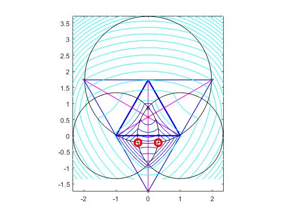
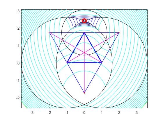
(a)                    (b)

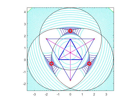
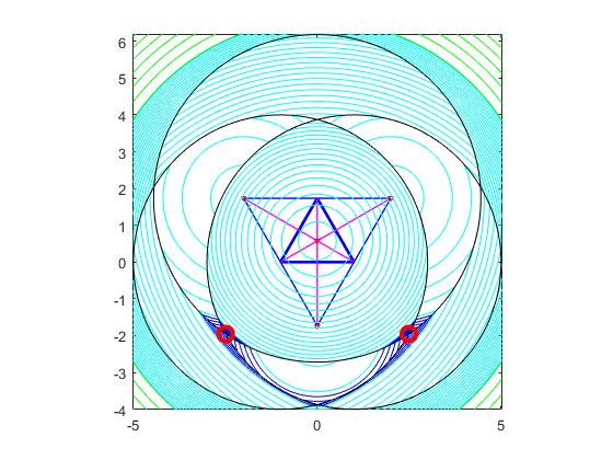
(c)                    (d)

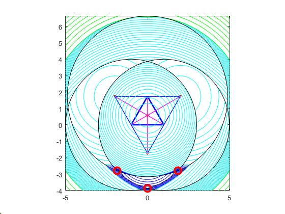
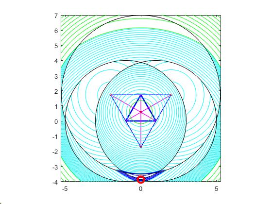
(e)                    (f)

Figure 4: Source locations when the measurement triangle is equilateral with $r=2$ (Theorem 11) and when $(d_{1},d_{3})=$ (a) $(1.3333,1.9737)$ (b) $(2.6000,1.3000)$ (c) $(2.6000,2.6000)$ (d) $(4.0000,4.4495)$ (e)$(4.000,4.8990)$ (f)$(4.000,5.2520)$.

	$O(S_{12+})$	$O(S_{31+})$	$O(S_{23+})$	$O(S_{12-})$	$O(S_{31-})$	$O(S_{23-})$
Fig. 4 (a)	3.1726	1.2628	1.2628	2.9375	7.3803	7.3803
Fig. 4 (b)	1.2438	4.9420	4.9420	15.3838	3.8720	3.8720
Fig. 4 (c)	6.3138	6.3138	6.3138	10.3138	10.3138	10.3138
Fig. 4 (d)	15.2144	9.9563	9.9563	11.6184	17.7543	17.7543
Fig. 4 (e)	19.4164	7.4164	7.4164	7.4164	19.4164	19.4164
Fig. 4 (f)	23.0000	4.4093	4.4093	3.8328	19.9929	19.9929

Table 3: The comparison of objective values at $S_{12\pm},S_{31\pm},$ and $S_{23\pm}$ for the equilateral triangle with $r=2$.

5 When the measurement triangle is isosceles

We will suppose that the measurement triangle is an isosceles triangle with $\left\lVert Z_{1}Z_{3}\right\rVert=\left\lVert Z_{2}Z_{3}\right\rVert$ and $d_{1}=d_{2}$. Let $r:=\left\lVert Z_{1}Z_{2}\right\rVert$ and $s:=\left\lVert Z_{3}-\frac{Z_{1}+Z_{2}}{2}\right\rVert$. Further, we will take into account the case that $d_{1}\geq\sqrt{\frac{r^{2}}{4}+\frac{s^{2}}{9}}$ and $d_{3}\in\left(\left|s-\sqrt{d_{1}^{2}-\frac{r^{2}}{4}}\right|,s+\sqrt{d_{1}^{2}-\frac{r^{2}}{4}}\right)$ for Lemma 12,13,14, and 15. This implies that $Y_{0}\in D_{1}\cap D_{2}$ and all three disks meet, and $R_{i_{1}i_{2}i_{3}}$ has one connected component for every $i_{1},i_{2},i_{3}\in\{0,1\}$ and thus, we have $X\subset S_{123}^{\pm}$ by Theorem 1.

Lemma 12.

Let $R$ be a positive constant such that

$$R^{2}:=d_{1}^{2}-\frac{r^{2}}{4}+s^{2}\frac{4s^{2}+r^{2}}{4s^{2}+9r^{2}}-2s\sqrt{d_{1}^{2}-\frac{r^{2}}{4}}\frac{4s^{2}-3r^{2}}{4s^{2}+9r^{2}},$$

then $R\in\left(\left|s-\sqrt{d_{1}^{2}-\frac{r^{2}}{4}}\right|,s+\sqrt{d_{1}^{2}-\frac{r^{2}}{4}}\right)$ and we have

$$\begin{array}[]{ccc}O(S_{31+})>O(S_{12+}),&{\mbox{i}ff}&d_{3}<R,\\ O(S_{31+})=O(S_{12+}),&{\mbox{i}ff}&d_{3}=R,\\ O(S_{31+})<O(S_{12+}),&{\mbox{i}ff}&d_{3}>R.\end{array}$$

Further, depending on $s/r$ and $d_{1}$, we have the following relations:

$$\begin{array}[]{ll}{\mbox{I}f}\;s=\frac{\sqrt{3}}{2}r,&{\mbox{t}hen}\;R=d_{1}.\\ &\\ {\mbox{I}f}\;s>\frac{\sqrt{3}}{2}r\;{\mbox{a}nd}&\left\{\begin{array}[]{ccc}d_{1}>\sqrt{\frac{r^{2}}{4}+s^{2}\left(\frac{4s^{2}+5r^{2}}{4s^{2}-3r^{2}}\right)^{2}},&{\mbox{t}hen}&\left|s-\sqrt{d_{1}^{2}-\frac{r^{2}}{4}}\right|<R<\sqrt{d_{1}^{2}-\frac{r^{2}}{4}-s^{2}},\\ d_{1}=\sqrt{\frac{r^{2}}{4}+s^{2}\left(\frac{4s^{2}+5r^{2}}{4s^{2}-3r^{2}}\right)^{2}},&{\mbox{t}hen}&R=\sqrt{d_{1}^{2}-\frac{r^{2}}{4}-s^{2}},\\ d_{1}<\sqrt{\frac{r^{2}}{4}+s^{2}\left(\frac{4s^{2}+5r^{2}}{4s^{2}-3r^{2}}\right)^{2}},&{\mbox{t}hen}&\sqrt{d_{1}^{2}-\frac{r^{2}}{4}-s^{2}}<R<\sqrt{d_{1}^{2}-\frac{r^{2}}{4}+s^{2}}.\end{array}\right.\\ &\\ {\mbox{I}f}\;s<\frac{\sqrt{3}}{2}r\;{\mbox{a}nd}&\left\{\begin{array}[]{ccc}d_{1}>\sqrt{\frac{r^{2}}{4}+s^{2}\left(\frac{4r^{2}}{3r^{2}-4s^{2}}\right)^{2}},&{\mbox{t}hen}&\sqrt{d_{1}^{2}-\frac{r^{2}}{4}+s^{2}}<R<s+\sqrt{d_{1}^{2}-\frac{r^{2}}{4}},\\ d_{1}=\sqrt{\frac{r^{2}}{4}+s^{2}\left(\frac{4r^{2}}{3r^{2}-4s^{2}}\right)^{2}},&{\mbox{t}hen}&R=\sqrt{d_{1}^{2}-\frac{r^{2}}{4}+s^{2}},\\ d_{1}<\sqrt{\frac{r^{2}}{4}+s^{2}\left(\frac{4r^{2}}{3r^{2}-4s^{2}}\right)^{2}},&{\mbox{t}hen}&\sqrt{d_{1}^{2}-\frac{r^{2}}{4}-s^{2}}<R<\sqrt{d_{1}^{2}-\frac{r^{2}}{4}+s^{2}}.\end{array}\right.\end{array}$$ (10)

Proof.

Let us compute $d_{3}=R$ satisfying $\left\lVert Y_{0}-S_{12+}\right\rVert=\left\lVert Y_{0}-S_{23+}\right\rVert=\left\lVert Y_{0}-S_{31+}\right\rVert$, which implies $O(S_{12+})=O(S_{23+})=O(S_{31+})$. By using Lemma 8

$$R^{2} = \left(\frac{2}{3}s\right)^{2}+\left(\sqrt{d_{1}^{2}-\frac{r^{2}}{4}}-\frac{s}{3}\right)^{2}-2\frac{2}{3}s\left(\sqrt{d_{1}^{2}-\frac{r^{2}}{4}}-\frac{s}{3}\right)\cos\angle Z_{3}Y_{0}S_{23+}$$

$$= d_{1}^{2}+\frac{5}{9}s^{2}-\frac{r^{2}}{4}-\frac{2}{3}s\sqrt{d_{1}^{2}-\frac{r^{2}}{4}}-\frac{4}{3}s\left(\sqrt{d_{1}^{2}-\frac{r^{2}}{4}}-\frac{s}{3}\right)\left(2\left(\frac{s/3}{\sqrt{\frac{r^{2}}{4}+\frac{s^{2}}{9}}}\right)^{2}-1\right)$$

$$= d_{1}^{2}-\frac{r^{2}}{4}+s^{2}\frac{4s^{2}+r^{2}}{4s^{2}+9r^{2}}-2s\sqrt{d_{1}^{2}-\frac{r^{2}}{4}}\frac{4s^{2}-3r^{2}}{4s^{2}+9r^{2}},$$

which proves the lemma. Here, we have used $\angle Z_{3}Y_{0}S_{23+}=\angle Z_{1}Y_{0}Z_{2}=2\angle Z_{1}Y_{0}L$, which is from (6). The computation of (10) is trivial. ∎

Lemma 13.

Suppose that $d_{1}\geq\sqrt{\frac{r^{2}}{4}+s^{2}}$. Let $M$ be a positive number such that

$$M^{2}:=d_{1}^{2}-\frac{r^{2}}{4}+2s\sqrt{d_{1}^{2}-\frac{r^{2}}{4}}\frac{4s^{2}-3r^{2}}{4s^{2}+r^{2}}+s^{2}\frac{4s^{2}+9r^{2}}{4s^{2}+r^{2}}.$$

Then, $M\in\left(\sqrt{d_{1}^{2}-\frac{r^{2}}{4}}-s,\sqrt{d_{1}^{2}-\frac{r^{2}}{4}}+s\right)$ and we have

$$\begin{array}[]{ccc}O(S_{31+})<O(S_{12-}),&{\mbox{i}ff}&d_{3}<M,\\ O(S_{31+})=O(S_{12-}),&{\mbox{i}ff}&d_{3}=M,\\ O(S_{31+})>O(S_{12-}),&{\mbox{i}ff}&d_{3}>M\end{array}$$

And further, we have the following inequalities about $M$:

$$\begin{array}[]{ll}{\mbox{I}f}\;s=\frac{\sqrt{3}}{2}r,&{\mbox{t}hen}\;M=\sqrt{d_{1}^{2}+2r^{2}}.\\ &\\ {\mbox{I}f}\;s>\frac{\sqrt{3}}{2}r,&{\mbox{t}hen}\;M>\sqrt{d_{1}^{2}-\frac{r^{2}}{4}+s^{2}}.\\ &\\ {\mbox{I}f}\;s<\frac{\sqrt{3}}{2}r\;{\mbox{a}nd}&\left\{\begin{array}[]{ccc}d_{1}>\sqrt{\frac{r^{2}}{4}+s^{2}\left(\frac{4r^{2}}{3r^{2}-4s^{2}}\right)^{2}},&{\mbox{t}hen}&M<\sqrt{d_{1}^{2}-\frac{r^{2}}{4}+s^{2}},\\ d_{1}=\sqrt{\frac{r^{2}}{4}+s^{2}\left(\frac{4r^{2}}{3r^{2}-4s^{2}}\right)^{2}},&{\mbox{t}hen}&M=\sqrt{d_{1}^{2}-\frac{r^{2}}{4}+s^{2}},\\ d_{1}<\sqrt{\frac{r^{2}}{4}+s^{2}\left(\frac{4r^{2}}{3r^{2}-4s^{2}}\right)^{2}},&{\mbox{t}hen}&M>\sqrt{d_{1}^{2}-\frac{r^{2}}{4}+s^{2}}.\\ \end{array}\right.\end{array}$$

.

Proof.

In this case, we have $Y_{3}\in R_{110}$. If we plot the circle centered at $Y_{3}$ with radius $\left\lVert Y_{3}-S_{12-}\right\rVert$, the circle meets $S_{1}$ and $S_{2}$ at one point except $S_{12-}$, respectively. Let this point be $M_{1}$ and $M_{2}$, respectively. Define $M:=\left\lVert Z_{3}-M_{1}\right\rVert=\left\lVert Z_{3}-M_{2}\right\rVert$. Let us compute $M$ in detail. Since $\left\lVert Z_{2}-M_{2}\right\rVert=\left\lVert Z_{2}-S_{12-}\right\rVert$ and $\left\lVert Y_{3}-M_{2}\right\rVert=\left\lVert Y_{3}-S_{12-}\right\rVert$, we have

$$\angle Z_{2}Y_{3}M_{2}=\angle Z_{2}Y_{3}M_{2}-\angle Z_{3}Y_{3}Z_{2}=\angle Z_{2}Y_{3}S_{12-}-\angle Z_{3}Y_{3}Z_{2}=\pi-2\angle Z_{3}Y_{3}Z_{2}.$$

Since $\cos\angle Z_{3}Y_{3}Z_{2}=\frac{s}{\sqrt{\frac{r^{2}}{4}+s^{2}}}$ and $\left\lVert M_{2}Y_{3}\right\rVert=\sqrt{d_{1}^{2}-\frac{r^{2}}{4}}-s$, we have

$$M^{2} = 4s^{2}+\left\lVert M_{2}Y_{3}\right\rVert^{2}-4s\left\lVert M_{2}Y_{3}\right\rVert\cos\angle Z_{3}Y_{3}M_{2}$$

$$= 4s^{2}+\left\lVert M_{2}Y_{3}\right\rVert^{2}-4s\left\lVert M_{2}Y_{3}\right\rVert(1-2\cos^{2}\angle Z_{3}Y_{3}Z_{2})$$

$$= d_{1}^{2}-\frac{r^{2}}{4}+2s\sqrt{d_{1}^{2}-\frac{r^{2}}{4}}\frac{4s^{2}-3r^{2}}{4s^{2}+r^{2}}+s^{2}\frac{4s^{2}+9r^{2}}{4s^{2}+r^{2}},$$

which proved the lemma. ∎

Note that the constant $P=\sqrt{\frac{r^{2}}{4}+s^{2}\left(\frac{4s^{2}+5r^{2}}{4s^{2}-3r^{2}}\right)^{2}}$ in Theorem 3 is only defined when $s>\frac{\sqrt{3}r}{2}$.

Lemma 14.

Assume that $d_{1}>\sqrt{\frac{r^{2}}{4}+s^{2}}$. Then, there is $d_{3}^{*}\in\left(\sqrt{d_{1}^{2}-\frac{r^{2}}{4}}-s,\sqrt{d_{1}^{2}-\frac{r^{2}}{4}-s^{2}}\right)$ when $s>\frac{\sqrt{3}}{2}r\mbox{ and }d_{1}>P$, such that

$${\mbox{I}f}\;\left(s\leq\frac{\sqrt{3}}{2}r\mbox{ or }d_{1}<P\right)&\mbox{ and }\;d_{3}\in\left[\sqrt{d_{1}^{2}-\frac{r^{2}}{4}}-s,\sqrt{d_{1}^{2}-\frac{r^{2}}{4}-s^{2}}\right],\;{\mbox{t}hen}\;O(S_{23-})>O(S_{12+}).{}\\ \\ {\mbox{I}f}\;s>\frac{\sqrt{3}}{2}r,d_{1}=P,\;{\mbox{a}nd}\left\{\begin{array}[]{ccc}d_{3}\in\left[\sqrt{d_{1}^{2}-\frac{r^{2}}{4}}-s,\sqrt{d_{1}^{2}-\frac{r^{2}}{4}-s^{2}}\right),&{\mbox{t}hen}\;O(S_{23-})>O(S_{12+}),\\ d_{3}=\sqrt{d_{1}^{2}-\frac{r^{2}}{4}-s^{2}},&{\mbox{t}hen}\;O(S_{23\pm})=O(S_{12+}).\\ \end{array}\right.{}\\ \\ {\mbox{I}f}s>\frac{\sqrt{3}}{2}r,d_{1}>P,\;{\mbox{a}nd}\left\{\begin{array}[]{ccc}d_{3}\in\left[\sqrt{d_{1}^{2}-\frac{r^{2}}{4}}-s,d_{3}^{*}\right),&{\mbox{t}hen}\;O(S_{23-})>O(S_{12+}),\\ d_{3}=d_{3}^{*},&{\mbox{t}hen}\;O(S_{23-})=O(S_{12+}),\\ d_{3}\in\left[d_{3}^{*},\sqrt{d_{1}^{2}-\frac{r^{2}}{4}-s^{2}}\right],&{\mbox{t}hen}\;O(S_{23-})<O(S_{12+}).\end{array}\right.{}$$ (11)

Proof.

Using

$$\cos\angle S_{31-}Z_{3}Z_{2}=\cos(\angle S_{31-}Z_{3}Z_{1}+2\angle Z_{1}Z_{3}L)=\frac{s^{2}-\frac{r^{2}}{4}}{s^{2}+\frac{r^{2}}{4}}\cos\angle S_{31-}Z_{3}Z_{1}-\frac{rs}{s^{2}+\frac{r^{2}}{4}}\sin\angle S_{31-}Z_{3}Z_{1},$$

let us compute $O(S_{12+})$ and $O(S_{31-})$ as follows:

$$O(S_{12+}) = d_{3}^{2}-\left\lVert Z_{3}-S_{12+}\right\rVert^{2}=d_{3}^{2}-\left(\sqrt{d_{1}^{2}-\frac{r^{2}}{4}}-s\right)^{2}=d_{3}^{2}-\left(d_{1}^{2}-\frac{r^{2}}{4}\right)-s^{2}+2s\sqrt{d_{1}^{2}-\frac{r^{2}}{4}}$$

$$O(S_{31-}) = -d_{2}^{2}+\left\lVert Z_{2}-S_{31-}\right\rVert^{2}=-d_{1}^{2}+\left(d_{3}^{2}+|Z_{1}Z_{3}|^{2}-2d_{3}|Z_{1}Z_{3}|\cos(\angle S_{31-}Z_{3}Z_{1}+\angle Z_{1}Z_{3}Z_{2})\right)$$

$$= d_{3}^{2}+|Z_{1}Z_{3}|^{2}-d_{1}^{2}-\frac{1}{|Z_{1}Z_{3}|^{2}}\left((d_{3}^{2}+|Z_{1}Z_{3}|^{2}-d_{1}^{2})(s^{2}-\frac{r^{2}}{4})-rs\sqrt{4d_{3}^{2}|Z_{1}Z_{3}|^{2}-(d_{3}^{2}+|Z_{1}Z_{3}|^{2}-d_{1}^{2})^{2}}\right)$$

Let $u=\sqrt{d_{1}^{2}-\frac{r^{2}}{4}}-s$. Then $u>0$. Next let us parametrize $d_{3}$ with respect to $t$ such as $d_{3}^{2}=u^{2}+2tsu$. Then we have $0\leq t\leq 1,0<u\leq d_{3}\leq u^{2}+2su,$ and $d_{3}^{2}-d_{1}^{2}+|Z_{1}Z_{3}|^{2}=2(t-1)su$. Inserting these parametrizatons into $O(S_{12+})$ and $O(S_{31-})$, we have the following function for $t\in[0,1]$.

$$g(t)=O(S_{31-})-O(S_{12+})=\frac{2s}{|Z_{1}Z_{3}|^{2}}\left(-u\left[\left(s^{2}-\frac{r^{2}}{4}\right)t+\frac{r^{2}}{2}\right]+r\sqrt{-s^{2}u^{2}t^{2}+2su(s^{2}+\frac{r^{2}}{4}+su)t+\frac{r^{2}u^{2}}{4}}\right)$$

Note that $g(0)=0$ and the first function on the right hand side is a linear function and the second function is an increasing concave function. Hence, we have $g^{\prime\prime}<0$ on $t\in[0,1]$. Therefore, under the condition that $g(1)>0$, we have $g(t)>0$ iff $t\in(0,1]$ and $g(1)=0$ implies $g(t)>0$ if and only if $t\in(0,1)$. And $g(1)<0$ implies that there is a $t^{*}$ in $(0,1)$ such that

$$\begin{array}[]{ccc}g(t)>0&\mbox{is equivalent to}&t\in(0,t^{*})\\ g(t)<0&\mbox{is equivalent to}&t\in(t^{*},1)\end{array}$$

Let $d_{3}^{*}=u^{2}+2t^{*}su,0<t^{*}<1$.

Let us find the condition on $u$ such that $g(1)=0$. From

$$g(1) = \frac{2s}{|Z_{1}Z_{3}|^{2}}\left(-u\left(s^{2}+\frac{r^{2}}{4}\right)+r\sqrt{\left(s^{2}+\frac{r^{2}}{4}\right)(u^{2}+2su)}\right)$$

$$= \frac{2sr\sqrt{u}}{|Z_{1}Z_{3}|}\left(\sqrt{u+2s}-\frac{\sqrt{s^{2}+\frac{r^{2}}{4}}}{r}\sqrt{u}\right)$$

we have,

$$\begin{array}[]{ccc}g(1)>0&\longleftrightarrow&s\leq\frac{\sqrt{3}}{2}r\mbox{ or }u<Q\\ g(1)=0&\longleftrightarrow&s>\frac{\sqrt{3}}{2}r\mbox{ and }u=Q\\ g(1)<0&\longleftrightarrow&s>\frac{\sqrt{3}}{2}r\mbox{ and }u>Q\end{array}$$

where $Q:=\frac{2r^{2}s}{s^{2}-\frac{3}{4}r^{2}}$. Since $u=Q$ implies $d_{1}=P$ and vice versa, we have proved the lemma. ∎

Theorem 15.

Suppose that $\left\lVert Z_{1}-Z_{3}\right\rVert=\left\lVert Z_{2}-Z_{3}\right\rVert$ and $d_{1}=d_{2}$. Then, the source $X$ is determined as follows:

s	$d_{1}=d_{2}$	$d_{3}$	$X$
$(0,\infty)$	$\left(0,\sqrt{\frac{r^{2}}{4}+\frac{s^{2}}{9}}\right]$	$\left(0,\frac{2s}{3}\right]$	$Y_{0}$
	$\left(0,\sqrt{\frac{r^{2}}{4}+s^{2}}\right]$	$\left[2s,\infty\right)$	$Y_{3}$
	$\left(0,\frac{r}{2}\right]$	$\left[\frac{2s}{3},2s\right]$	$N_{3}$
	$\left(\frac{r}{2},\sqrt{\frac{r^{2}}{4}+\frac{s^{2}}{9}}\right]$	$\left[\frac{2s}{3},s-\sqrt{d_{1}^{2}-\frac{r^{2}}{4}}\right]$	$N_{3}$
	$\left(\frac{r}{2},\sqrt{\frac{r^{2}}{4}+s^{2}}\right]$	$\left[s+\sqrt{d_{1}^{2}-\frac{r^{2}}{4}},2s\right]$	$N_{3}$
	$\left(\frac{r}{2},\sqrt{\frac{r^{2}}{4}+\frac{s^{2}}{9}}\right)$	$\left(s-\sqrt{d_{1}^{2}-\frac{r^{2}}{4}},s+\sqrt{d_{1}^{2}-\frac{r^{2}}{4}}\right)$	$\{S_{23+},S_{31+}\}$
	$\left[\sqrt{\frac{r^{2}}{4}+\frac{s^{2}}{9}},\infty\right)$	$\left(0,\left|s-\sqrt{d_{1}^{2}-\frac{r^{2}}{4}}\right|\right]$	$S_{12+}$
	$\left[\sqrt{\frac{r^{2}}{4}+\frac{s^{2}}{9}},\sqrt{\frac{r^{2}}{4}+s^{2}}\right)$	$\left[s-\sqrt{d_{1}^{2}-\frac{r^{2}}{4}},R\right)$	$S_{12+}$
		$R$	$\{S_{12+},S_{23+},S_{31+}\}$
		$\left(R,s+\sqrt{d_{1}^{2}-\frac{r^{2}}{4}}\right]$	$\{S_{23+},S_{31+}\}$
$\left(0,\frac{\sqrt{3}r}{2}\right)$	$\left[\sqrt{\frac{r^{2}}{4}+s^{2}},\sqrt{\frac{r^{2}}{4}+s^{2}\left(\frac{4r^{2}}{3r^{2}-4s^{2}}\right)^{2}}\right)$	$\left[\sqrt{d_{1}^{2}-\frac{r^{2}}{4}}-s,R\right)$	$S_{12+}$
		$R$	$S_{123}^{+}$
		$\left(R,M\right)$	$\{S_{23+},S_{31+}\}$
		$M$	$\{S_{23+},S_{31+},S_{12-}\}$
		$\left(M,\infty\right)$	$S_{12-}$
	$\sqrt{\frac{r^{2}}{4}+s^{2}\left(\frac{4r^{2}}{3r^{2}-4s^{2}}\right)^{2}}$	$\left[\sqrt{d_{1}^{2}-\frac{r^{2}}{4}}-s,\sqrt{d_{1}^{2}-\frac{r^{2}}{4}+s^{2}}\right)$	$S_{12+}$
		$\sqrt{d_{1}^{2}-\frac{r^{2}}{4}+s^{2}}$	$\{S_{12\pm},S_{23+},S_{31+}\}$
		$\left(\sqrt{d_{1}^{2}-\frac{r^{2}}{4}+s^{2}},\infty\right)$	$S_{12-}$
	$\left(\sqrt{\frac{r^{2}}{4}+s^{2}\left(\frac{4r^{2}}{3r^{2}-4s^{2}}\right)^{2}},\infty\right)$	$\left[\sqrt{d_{1}^{2}-\frac{r^{2}}{4}}-s,\sqrt{d_{1}^{2}-\frac{r^{2}}{4}+s^{2}}\right)$	$S_{12+}$
		$\sqrt{d_{1}^{2}-\frac{r^{2}}{4}+s^{2}}$	$S_{12\pm}$
		$\left(\sqrt{d_{1}^{2}-\frac{r^{2}}{4}+s^{2}},\infty\right)$	$S_{12-}$

s	$d_{1}=d_{2}$	$d_{3}$	$X$
$\left(\frac{\sqrt{3}r}{2},\infty\right)$	$\left[\sqrt{\frac{r^{2}}{4}+s^{2}},\sqrt{\frac{r^{2}}{4}+s^{2}\left(\frac{4s^{2}+5r^{2}}{4s^{2}-3r^{2}}\right)^{2}}\right)$	$\left[\sqrt{d_{1}^{2}-\frac{r^{2}}{4}}-s,R\right)$	$S_{12+}$
		$R$	$S_{123}^{+}$
		$\left[R,\sqrt{d_{1}^{2}-\frac{r^{2}}{4}-s^{2}}\right)$	$\{S_{23+},S_{31+}\}$
	$\sqrt{\frac{r^{2}}{4}+s^{2}\left(\frac{4s^{2}+5r^{2}}{4s^{2}-3r^{2}}\right)^{2}}$	$\left[\sqrt{d_{1}^{2}-\frac{r^{2}}{4}}-s,\sqrt{d_{1}^{2}-\frac{r^{2}}{4}-s^{2}}\right)$	$S_{12+}$
		$\sqrt{d_{1}^{2}-\frac{r^{2}}{4}-s^{2}}$	$\{S_{12+},S_{23\pm},S_{31\pm}\}$
		$\left(\sqrt{d_{1}^{2}-\frac{r^{2}}{4}-s^{2}},\sqrt{d_{1}^{2}-\frac{r^{2}}{4}+s^{2}}\right]$	$\{S_{23+},S_{31+}\}$
	$\left(\sqrt{\frac{r^{2}}{4}+s^{2}\left(\frac{4s^{2}+5r^{2}}{4s^{2}-3r^{2}}\right)^{2}},\infty\right)$	$\left(\sqrt{d_{1}^{2}-\frac{r^{2}}{4}}-s,d_{3}^{*}\right)$	$S_{12+}$
		$d_{3}^{*}$	$\{S_{12+},S_{23-},S_{31-}\}$
		$\left(d_{3}^{*},\sqrt{d_{1}^{2}-\frac{r^{2}}{4}+s^{2}}\right)$	$\{S_{23-},S_{31-}\}$
		$\sqrt{d_{1}^{2}-\frac{r^{2}}{4}+s^{2}}$	$\{S_{23\pm},S_{31\pm}\}$
	$\left[\sqrt{\frac{r^{2}}{4}+s^{2}},\infty\right)$	$\left(\sqrt{d_{1}^{2}-\frac{r^{2}}{4}+s^{2}},M\right)$	$\{S_{23+},S_{31+}\}$
		$M$	$\{S_{23+},S_{31+},S_{12-}\}$
		$\left(M,\infty\right)$	$S_{12-}$

Proof.

The proofs for the cases $X=Y_{0},X=Y_{3},$ and $X=N_{3}$ are similar to that of Lemma 11.

If $d_{1}\geq\sqrt{\frac{r^{2}}{4}+\frac{s^{2}}{9}}$ and $d_{3}\leq\left|s-\sqrt{d_{1}^{2}-\frac{r^{2}}{4}}\right|$ , then $X=S_{12+}$ by similar argument as Lemma 11.

If $d_{1}\geq\sqrt{\frac{r^{2}}{4}+s^{2}}$ and $d_{3}\geq s+\sqrt{d_{1}^{2}-\frac{r^{2}}{4}}$ , then $X=S_{12-}$ also by similar argument as Lemma 11.

If $d_{1}\in\left(\frac{r}{2},\sqrt{\frac{r^{2}}{4}+\frac{s^{2}}{9}}\right)$ and $d_{3}\in\left(s-\sqrt{d_{1}^{2}-\frac{r^{2}}{4}},s+\sqrt{d_{1}^{2}-\frac{r^{2}}{4}}\right)$, then all three disks meet and $R_{i_{1}i_{2}i_{3}}$ has one connected component for every $i_{1},i_{2},i_{3}\in\{0,1\}$ and we have $X\geq S_{123}^{\pm}$ by Theorem 1. Using Lemma 6 and the similar argument as Lemma 11, we have $X=\{S_{23+},S_{31+}\}$.

The remaining cases are when $d_{1}\geq\sqrt{\frac{r^{2}}{4}+\frac{s^{2}}{9}}$ and $d_{3}\in\left(\left|s-\sqrt{d_{1}^{2}-\frac{r^{2}}{4}}\right|,s+\sqrt{d_{1}^{2}-\frac{r^{2}}{4}}\right)$. In this all three disks meet and $R_{i_{1}i_{2}i_{3}}$ has one connected component for every $i_{1},i_{2},i_{3}\in\{0,1\}$ and we have $X\geq S_{123}^{\pm}$ by Theorem 1. Using Lemma 6, we have

$$&\mbox{If }\sqrt{\frac{r^{2}}{4}+\frac{s^{2}}{9}}\leq d_{1}<\sqrt{\frac{r^{2}}{4}+s^{2}}\mbox{ and }d_{3}\in\left(s-\sqrt{d_{1}^{2}-\frac{r^{2}}{4}},\sqrt{d_{1}^{2}-\frac{r^{2}}{4}+s^{2}}\right),\\ \mbox{ then }X\subset\{S_{12+},S_{23+},S_{31+}\}.{}\\ \mbox{If }d_{1}>\sqrt{\frac{r^{2}}{4}+s^{2}}\mbox{ and }d_{3}\in\left(\sqrt{d_{1}^{2}-\frac{r^{2}}{4}}-s,\sqrt{d_{1}^{2}-\frac{r^{2}}{4}-s^{2}}\right),\mbox{ then }X\subset\{S_{12+},S_{23-},S_{31-}\}.{}\\ \mbox{If }d_{1}>\sqrt{\frac{r^{2}}{4}+s^{2}}\mbox{ and }d_{3}=\sqrt{d_{1}^{2}-\frac{r^{2}}{4}-s^{2}},\mbox{ then }X\subset\{S_{12+},S_{23\pm},S_{31\pm}\}.{}\\ \mbox{If }d_{1}>\sqrt{\frac{r^{2}}{4}+s^{2}}\mbox{ and }d_{3}\in\left(\sqrt{d_{1}^{2}-\frac{r^{2}}{4}-s^{2}},\sqrt{d_{1}^{2}-\frac{r^{2}}{4}+s^{2}}\right),\mbox{ then }X\subset\{S_{12+},S_{23+},S_{31+}\}.{}\\ \mbox{If }d_{3}=\sqrt{d_{1}^{2}-\frac{r^{2}}{4}+s^{2}},\mbox{ then }X\subset\{S_{12\pm},S_{23+},S_{31+}\}.{}\\ \mbox{If }d_{3}\in\left(\sqrt{d_{1}^{2}-\frac{r^{2}}{4}+s^{2}},s+\sqrt{d_{1}^{2}-\frac{r^{2}}{4}}\right),\mbox{ then }X\subset\{S_{23+},S_{31+},S_{12-}\}.{}$$ (12)

When $d_{1}\in\left[\sqrt{\frac{r^{2}}{4}+\frac{s^{2}}{9}},\sqrt{\frac{r^{2}}{4}+s^{2}}\right)$ and $d_{3}\in\left(\sqrt{d_{1}^{2}-\frac{r^{2}}{4}+s^{2}},s+\sqrt{d_{1}^{2}-\frac{r^{2}}{4}}\right)$, by using (LABEL:eq:SAclassify6) we have $X\geq X_{001}$. Since the minimum points are the farthest points from $Y_{3}$ and $Y_{3}$ is not contained in $R_{001}$, we have $X=X_{001}=\{S_{23+},S_{31+}\}$. Note that in case (LABEL:eq:SAclassify1), the constant $R$ in Lemma 12 satisfies

$$s-\sqrt{d_{1}^{2}-\frac{r^{2}}{4}}<R<\sqrt{d_{1}^{2}-\frac{r^{2}}{4}+s^{2}}.$$

From the above and by using (LABEL:eq:SAclassify5) and Lemma 12, we can prove all the case for $d_{1}\in\left[\sqrt{\frac{r^{2}}{4}+\frac{s^{2}}{9}},\sqrt{\frac{r^{2}}{4}+s^{2}}\right)$ and $d_{3}\in\left(\sqrt{d_{1}^{2}-\frac{r^{2}}{4}+s^{2}},s+\sqrt{d_{1}^{2}-\frac{r^{2}}{4}}\right)$.

Thus far, we have proved all the cases except $d_{1}\geq\sqrt{\frac{r^{2}}{4}+s^{2}}$ and $d_{3}\in\left[\sqrt{d_{1}^{2}-\frac{r^{2}}{4}}-s,\sqrt{d_{1}^{2}-\frac{r^{2}}{4}+s^{2}}\right]$. In the case, we should divide the original case into two cases: the flat isosceles ($s<\frac{\sqrt{3}r}{2}$) and the sharp isosceles ($s>\frac{\sqrt{3}r}{2}$) .

Let us consider the flat isosceles with $s<\frac{\sqrt{3}}{2}r$. In the case in (LABEL:eq:SAclassify2), we have $X\subset\{S_{12+},S_{23-},S_{31-}\}$. Using (LABEL:eq:S12+S23-1), we have $X=S_{12+}$. In the other cases, by applying Lemma 12, Lemma 13, and (LABEL:eq:SAclassify3)-(LABEL:eq:SAclassify6), we can prove all the cases for $s<\frac{\sqrt{3}}{2}r$.

Then, let us consider the sharp isosceles with $s>\frac{\sqrt{3}}{2}r$. The case $d_{1}\geq\sqrt{\frac{r^{2}}{4}+s^{2}}$ and $d_{3}\geq\sqrt{d_{1}^{2}-\frac{r^{2}}{4}+s^{2}}$ can be proved with Lemma 13, (LABEL:eq:SAclassify5), and (LABEL:eq:SAclassify6). In the other cases, by applying Lemma 12, Lemma 13, (LABEL:eq:S12+S23-2),(LABEL:eq:S12+S23-3), and (LABEL:eq:SAclassify3)-(LABEL:eq:SAclassify6), we can prove all the cases for $s<\frac{\sqrt{3}}{2}r$.

Hence, we proved all the cases of the theorem. ∎

In Fig. 5, 6, and 7, interesting examples when $R_{i1,i2,i3}$ are all nonempty and connected for $i_{1},i_{2},i_{3}\in\{0,1\}$ are shown in Theorem le:isoscelesd12. The objective values for the cases shown in the figures are displayed in Table 4, in which red ones in each row represent the objective values for the solutions in each case.

	$O(S_{12+})$	$O(S_{31+})$	$O(S_{23+})$	$O(S_{12-})$	$O(S_{31-})$	$O(S_{23-})$
Fig. 5 (a)	2.8643	2.8643	2.8643	3.2429	6.4858	6.4858
Fig. 5 (b)	3.4103	2.5370	2.5370	2.6969	7.2504	7.2504
Fig. 5 (c)	0.5567	4.6636	4.6636	7.4433	1.7770	1.7770
Fig. 5 (d)	4.0000	4.0000	4.0000	4.0000	8.0000	8.0000
Fig. 5 (e)	4.0491	13.4171	13.4171	13.3865	8.0797	8.0797
Fig. 5 (f)	8.7178	10.4900	10.4900	8.7178	14.4900	14.4900
Fig. 6 (a)	6.5105	12.9986	12.9986	53.7055	10.7596	10.7596
Fig. 6 (b)	16.0720	16.0720	16.0720	44.1440	17.6576	17.6576
Fig. 6 (c)	22.6289	16.4606	16.4606	37.5872	20.6689	20.6689
Fig. 6 (d)	10.6491	20.5469	20.5469	73.3509	15.2066	15.2066
Fig. 6 (e)	24.0000	24.0000	24.0000	60.0000	24.0000	24.0000
Fig. 6 (f)	32.5832	24.2271	24.2271	51.4168	27.6604	27.6604
Fig. 7 (a)	28.6572	36.0460	36.0460	94.5497	30.0675	30.0675
Fig. 7 (b)	31.8414	36.5462	36.5462	91.3655	31.8414	31.8414
Fig. 7 (c)	42.4272	37.2617	37.2617	80.7797	36.7912	36.7912

Table 4: The comparison of objective values at $S_{12\pm},S_{31\pm},$ and $S_{23\pm}$ for Theorem 15. The red numbers are the minimum objective values.

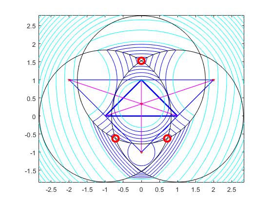
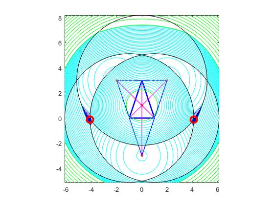
(a)                    (b)

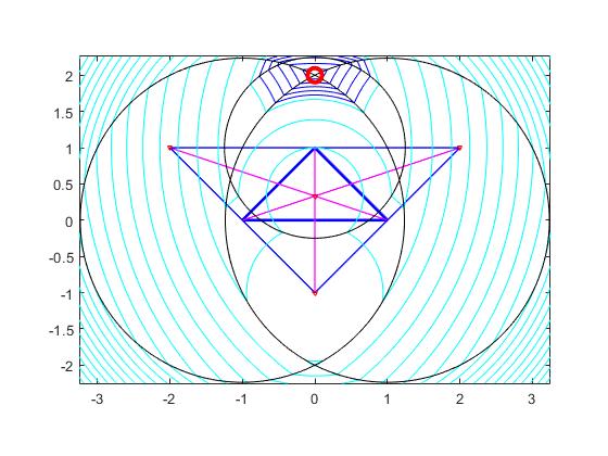
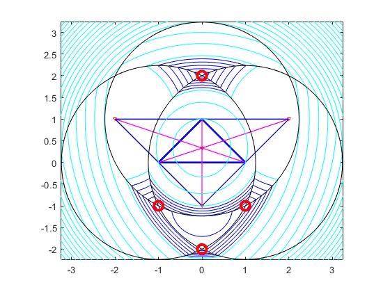
(c)                    (d)

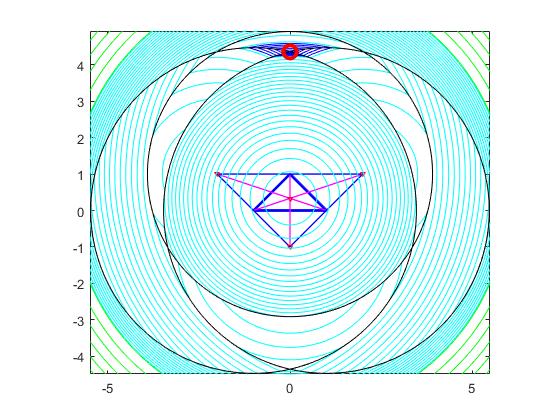
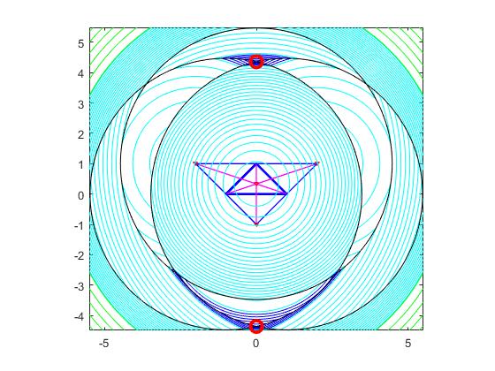
(e)                    (f)

Figure 5: Solution positions for flat isoscleles $(s<\frac{\sqrt{3}r}{2})$ with $s=1$ and $r=2$ in Theorem 15, when $(d_{1},d_{3})=$ (a) $(1.8251,1.7725)$ (b) $(1.8251,1.9204)$ (c) $(2.2361,1.2477)$ (d) $(2.2361,2.2361)$ (e) $(4.4721,3.9155)$ (f) $(4.4721,4.4721)$.

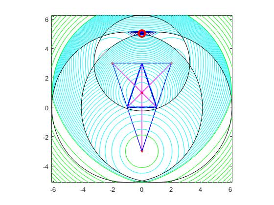
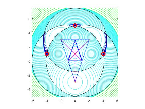
(a)                    (b)

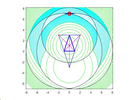
(c)                    (d)

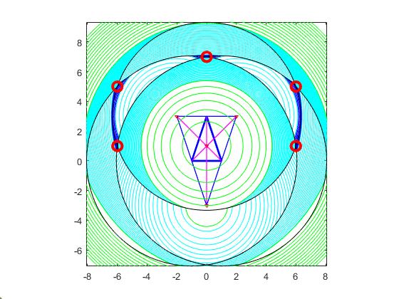
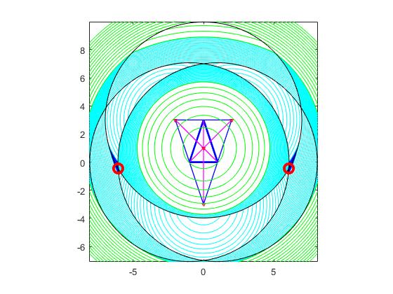
(e)                    (f)

Figure 6: Solution positions for sharp isosceles $(s>\frac{\sqrt{3}r}{2})$ with $s=3,\;r=2,$ and $\sqrt{\frac{r^{2}}{4}+s^{2}}\leq d_{1}\leq\sqrt{\frac{r^{2}}{4}+s^{2}\left(\frac{4s^{2}+5r^{2}}{4s^{2}-3r^{2}}\right)^{2}}$ (Theorem 15) when $(d_{1},d_{3})=$ (a) $(5.1167,3.2531)$ (b) $(5.1167,4.4882)$ (c) $(5.1167,5.1673)$ (d) $(7.0711,5.1623)$ (e) $(7.0711,6.3246)$ (f) $(7.0711,6.9702)$.

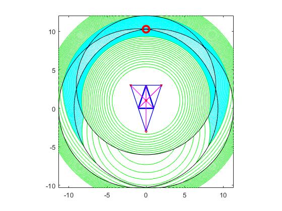
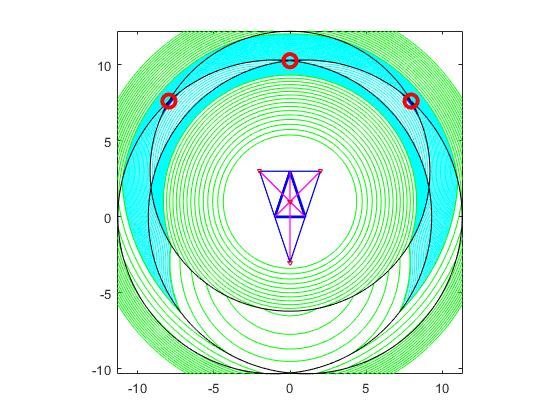
(a)                    (b)

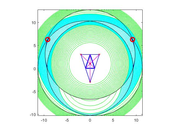
(c)                    (d)

Figure 7: Solution positions for sharp isosceles $(s>\frac{\sqrt{3}r}{2})$ with $s=3,r=2,\;\sqrt{\frac{r^{2}}{4}+s^{2}\left(\frac{4s^{2}+5r^{2}}{4s^{2}-3r^{2}}\right)^{2}}<d_{1}=10.3158\leq P$ (Theorem 15) and $d_{3}^{*}=9.2008$ when (a) $d_{3}=9.0261<d_{3}^{*}$ (b) $d_{3}=d_{3}^{*}$ (c) $d_{3}=9.7591>d_{3}^{*}$. (d) The graph for $f(t)$ in Lemma 14, in which the $x$-intercept point of $f(t)$ is $t^{*}=0.7302$ (up to 4 decimals).

Corollary 16.

Suppose that $\left\lVert Z_{1}-Z_{3}\right\rVert=\left\lVert Z_{2}-Z_{3}\right\rVert$ and $d_{1}=d_{2}$. Then, we have the followings:

• $X=\{S_{12+},S_{23\pm},S_{31\pm}\}$ iff $\left[s>\frac{\sqrt{3}}{2}r,d_{1}=\sqrt{\frac{r^{2}}{4}+s^{2}\left(\frac{4s^{2}+5r^{2}}{4s^{2}-3r^{2}}\right)^{2}},d_{3}=\frac{4sr}{4s^{2}-3r^{2}}\sqrt{4s^{2}+r^{2}}\right]$.

• $X=\{S_{23\pm},S_{31\pm}\}$ iff $\left[s>\frac{\sqrt{3}}{2}r,d_{1}>\sqrt{\frac{r^{2}}{4}+s^{2}\left(\frac{4s^{2}+5r^{2}}{4s^{2}-3r^{2}}\right)^{2}},d_{3}=\sqrt{d_{1}^{2}-\frac{r^{2}}{4}-s^{2}}\right]$.

• $X=\{S_{12\pm},S_{23+},S_{31+}\}$ iff $\left[s<\frac{\sqrt{3}}{2}r,d_{1}=\sqrt{\frac{r^{2}}{4}+s^{2}\left(\frac{4r^{2}}{3r^{2}-4s^{2}}\right)^{2}},d_{3}=\frac{\sqrt{25r^{4}-24r^{2}s^{2}+16s^{4}}}{3r^{2}-4s^{2}}\right]$.

• $X=\{S_{12-},S_{23+},S_{31+}\}$ iff $\left[d_{1}>\sqrt{\frac{r^{2}}{4}+s^{2}},d_{3}=M\right]$.

• $X=\{S_{12+},S_{23-},S_{31-}\}$ iff $\left[s>\frac{\sqrt{3}}{2}r,d_{1}>\sqrt{\frac{r^{2}}{4}+s^{2}\left(\frac{4s^{2}+5r^{2}}{4s^{2}-3r^{2}}\right)^{2}},d_{3}=d_{3}^{*}\right]$.

• $X=\{S_{12+},S_{23+},S_{31+}\}$ iff $\left[\sqrt{\frac{r^{2}}{4}+\frac{s^{2}}{9}}<d_{1}<\sqrt{\frac{r^{2}}{4}+s^{2}},d_{3}=R\right]$, or $\left[s=\frac{\sqrt{3}r}{2}.d_{1}>r,d_{3}=d_{1}\right]$,
  or $\left[s<\frac{\sqrt{3}}{2}r,\sqrt{\frac{r^{2}}{4}+s^{2}}\leq d_{1}<\sqrt{\frac{r^{2}}{4}+s^{2}\left(\frac{4r^{2}}{3r^{2}-4s^{2}}\right)^{2}},d_{3}=R\right]$,
  or $\left[s>\frac{\sqrt{3}}{2}r,\sqrt{\frac{r^{2}}{4}+s^{2}}\leq d_{1}<\sqrt{\frac{r^{2}}{4}+s^{2}\left(\frac{4s^{2}+5r^{2}}{4s^{2}-3r^{2}}\right)^{2}},d_{3}=R\right]$.

• $X=S_{12\pm}$ iff $\left[s<\frac{\sqrt{3}}{2}r,d_{1}>\sqrt{\frac{r^{2}}{4}+s^{2}\left(\frac{4r^{2}}{3r^{2}-4s^{2}}\right)^{2}},d_{3}=\sqrt{d_{1}^{2}-\frac{r^{2}}{4}-s^{2}}\right]$.

• $X=\{S_{23-},S_{31-}\}$ iff $\left[s>\frac{\sqrt{3}}{2}r,d_{1}>\sqrt{\frac{r^{2}}{4}+s^{2}\left(\frac{4s^{2}+5r^{2}}{4s^{2}-3r^{2}}\right)^{2}},d_{3}^{*}<d_{3}<\sqrt{d_{1}^{2}-\frac{r^{2}}{4}-s^{2}}\right]$.

• $X=\{S_{23+},S_{31+}\}$ iff $\left[\frac{r}{2}<d_{1}<\sqrt{\frac{r^{2}}{4}+\frac{s^{2}}{9}},s-\sqrt{d_{1}^{2}-\frac{r^{2}}{4}}<d_{3}<s+\sqrt{d_{1}^{2}-\frac{r^{2}}{4}}\right]$,
  or $\left[\sqrt{\frac{r^{2}}{4}+\frac{s^{2}}{9}}<d_{1}\leq\sqrt{\frac{r^{2}}{4}+s^{2}},R<d_{3}<s+\sqrt{d_{1}^{2}-\frac{r^{2}}{4}}\right]$, or $\left[s=\frac{\sqrt{3}r}{2},d_{1}>r,R<d_{3}<\sqrt{d_{1}^{2}+2r^{2}}\right]$,
  or $\left[s<\frac{\sqrt{3}}{2}r,\sqrt{\frac{r^{2}}{4}+s^{2}}<d_{1}<\sqrt{\frac{r^{2}}{4}+s^{2}\left(\frac{4r^{2}}{3r^{2}-4s^{2}}\right)^{2}},R<d_{3}<M\right]$,
  or $\left[s>\frac{\sqrt{3}}{2}r,d_{1}>\sqrt{\frac{r^{2}}{4}+s^{2}},\max(R,\sqrt{d_{1}^{2}-\frac{r^{2}}{4}-s^{2}})<d_{3}<M\right]$.

Note that the cases in Corollary 16 are all the nonunique cases for the source $X$, when $\left\lVert Z_{1}-Z_{3}\right\rVert=\left\lVert Z_{2}-Z_{3}\right\rVert$ and $d_{1}=d_{2}$.

6 Appendix

We list the solutions in dictionary order for $d_{1}=d_{2}$ and $d_{3}$ in each cases for the isosceles measurement triangle with $|Z_{1}Z_{3}|=|Z_{2}Z_{3}|$. The number of solutions $|X|$ are also listed in the following tables. These results are the reorganization of Theorems 11 and 15.

6.1 Equilateral triangle case with $s=\frac{\sqrt{3}}{2}r$

This table is the reorganization of the table in Theorem 11.

$d_{1}=d_{2}$	$d_{3}$	$X$	$|X|$
$\left(0,\frac{r}{2}\right]$	$\left(0,\frac{r}{\sqrt{3}}\right]$	$Y_{0}$	1
	$\left[\frac{r}{\sqrt{3}},\sqrt{3}r\right]$	$N_{3}$	1
	$\left[\sqrt{3}r,\infty\right)$	$Y_{3}$	1
$\left(\frac{r}{2},\frac{r}{\sqrt{3}}\right]$	$\left(0,\frac{r}{\sqrt{3}}\right]$	$Y_{0}$	1
	$\left[\frac{r}{\sqrt{3}},\frac{\sqrt{3}}{2}r-\sqrt{d_{1}^{2}-\frac{r^{2}}{4}}\right]$	$N_{3}$	1
	$\left(\frac{\sqrt{3}}{2}r-\sqrt{d_{1}^{2}-\frac{r^{2}}{4}},\frac{\sqrt{3}}{2}r+\sqrt{d_{1}^{2}-\frac{r^{2}}{4}}\right)$	$\{S_{23+},S_{31+}\}$	2
	$\left[\frac{\sqrt{3}}{2}r+\sqrt{d_{1}^{2}-\frac{r^{2}}{4}},\sqrt{3}r\right]$	$N_{3}$	1
	$\left[\sqrt{3}r,\infty\right)$	$Y_{3}$	1
$\left(\frac{r}{\sqrt{3}},r\right]$	$\left(0,d_{1}\right)$	$S_{12+}$	1
	$d_{1}$	$\{S_{12+},S_{23+},S_{31+}\}$	3
	$\left(d_{1},\frac{\sqrt{3}}{2}r+\sqrt{d_{1}^{2}-\frac{r^{2}}{4}}\right)$	$\{S_{23+},S_{31+}\}$	2
	$\left[\frac{\sqrt{3}}{2}r+\sqrt{d_{1}^{2}-\frac{r^{2}}{4}},\sqrt{3}r\right]$	$N_{3}$	1
	$\left[\sqrt{3}r,\infty\right)$	$Y_{3}$	1
$\left(r,\infty\right)$	$\left(0,d_{1}\right)$	$S_{12+}$	1
	$d_{1}$	$\{S_{12+},S_{23+},S_{31+}\}$	3
	$\left(d_{1},\sqrt{d_{1}^{2}+2r^{2}}\right)$	$\{S_{23+},S_{31+}\}$	2
	$\sqrt{d_{1}^{2}+2r^{2}}$	$\{S_{23+},S_{31+},S_{12-}\}$	3
	$\left(\sqrt{d_{1}^{2}+2r^{2}},\infty\right)$	$S_{12-}$	1

6.2 Flat isoscele trianlge case with $s<\frac{\sqrt{3}}{2}r$

This table is the reorganization of the table in Theorem 15.

$d_{1}=d_{2}$	$d_{3}$	$X$	$|X|$
$\left(0,\frac{r}{2}\right]$	$\left(0,\frac{2s}{3}\right]$	$Y_{0}$	1
	$\left[\frac{2s}{3},2s\right]$	$N_{3}$	1
	$\left[2s,\infty\right)$	$Y_{3}$	1
$\left(\frac{r}{2},\sqrt{\frac{r^{2}}{4}+\frac{s^{2}}{9}}\right]$	$\left(0,\frac{2s}{3}\right]$	$Y_{0}$	1
	$\left[\frac{2s}{3},s-\sqrt{d_{1}^{2}-\frac{r^{2}}{4}}\right]$	$N_{3}$	1
	$\left(s-\sqrt{d_{1}^{2}-\frac{r^{2}}{4}},s+\sqrt{d_{1}^{2}-\frac{r^{2}}{4}}\right)$	$\{S_{23+},S_{31+}\}$	2
	$\left[s+\sqrt{d_{1}^{2}-\frac{r^{2}}{4}},2s\right]$	$N_{3}$	1
	$\left[2s,\infty\right)$	$Y_{3}$	1
$\left(\sqrt{\frac{r^{2}}{4}+\frac{s^{2}}{9}},\sqrt{\frac{r^{2}}{4}+s^{2}}\right]$	$\left(0,R\right)$	$S_{12+}$	1
	$R$	$\{S_{12+},S_{23+},S_{31+}\}$	3
	$\left(R,s+\sqrt{d_{1}^{2}-\frac{r^{2}}{4}}\right)$	$\{S_{23+},S_{31+}\}$	2
	$\left[s+\sqrt{d_{1}^{2}-\frac{r^{2}}{4}},2s\right]$	$N_{3}$	1
	$\left[2s,\infty\right)$	$Y_{3}$	1
$\left(\sqrt{\frac{r^{2}}{4}+s^{2}},\sqrt{\frac{r^{2}}{4}+s^{2}\left(\frac{4r^{2}}{3r^{2}-4s^{2}}\right)^{2}}\right)$	$\left(0,R\right)$	$S_{12+}$	1
	$R$	$S_{123}^{+}$	3
	$\left(R,M\right)$	$\{S_{23+},S_{31+}\}$	2
	$M$	$\{S_{23+},S_{31+},S_{12-}\}$	3
	$\left(M,\infty\right)$	$S_{12-}$	1
$\sqrt{\frac{r^{2}}{4}+s^{2}\left(\frac{4r^{2}}{3r^{2}-4s^{2}}\right)^{2}}$	$\left(0,\sqrt{d_{1}^{2}-\frac{r^{2}}{4}+s^{2}}\right)$	$S_{12+}$	1
	$\sqrt{d_{1}^{2}-\frac{r^{2}}{4}+s^{2}}$	$\{S_{12\pm},S_{23+},S_{31+}\}$	4
	$\left(\sqrt{d_{1}^{2}-\frac{r^{2}}{4}+s^{2}},\infty\right)$	$S_{12-}$	1
$\left(\sqrt{\frac{r^{2}}{4}+s^{2}\left(\frac{4r^{2}}{3r^{2}-4s^{2}}\right)^{2}},\infty\right)$	$\left(0,\sqrt{d_{1}^{2}-\frac{r^{2}}{4}+s^{2}}\right)$	$S_{12+}$	1
	$\sqrt{d_{1}^{2}-\frac{r^{2}}{4}+s^{2}}$	$S_{12\pm}$	2
	$\left(\sqrt{d_{1}^{2}-\frac{r^{2}}{4}+s^{2}},\infty\right)$	$S_{12-}$	1

6.3 Shapr isosceles triangle case with $s>\frac{\sqrt{3}}{2}r$

This table is also the reorganization of the table in Theorem 15.
$d_{1}=d_{2}$ $d_{3}$ $X$ $|X|$ $\left(0,\frac{r}{2}\right]$ $\left(0,\frac{2s}{3}\right]$ $Y_{0}$ 1 $\left[\frac{2s}{3},2s\right]$ $N_{3}$ 1 $\left[2s,\infty\right)$ $Y_{3}$ 1 $\left(\frac{r}{2},\sqrt{\frac{r^{2}}{4}+\frac{s^{2}}{9}}\right]$ $\left(0,\frac{2s}{3}\right]$ $Y_{0}$ 1 $\left[\frac{2s}{3},s-\sqrt{d_{1}^{2}-\frac{r^{2}}{4}}\right]$ $N_{3}$ 1 $\left(s-\sqrt{d_{1}^{2}-\frac{r^{2}}{4}},s+\sqrt{d_{1}^{2}-\frac{r^{2}}{4}}\right)$ $\{S_{23+},S_{31+}\}$ 2 $\left[s+\sqrt{d_{1}^{2}-\frac{r^{2}}{4}},2s\right]$ $N_{3}$ 1 $\left[2s,\infty\right)$ $Y_{3}$ 1 $\left(\sqrt{\frac{r^{2}}{4}+\frac{s^{2}}{9}},\sqrt{\frac{r^{2}}{4}+s^{2}}\right]$ $\left(0,R\right)$ $S_{12+}$ 1 $R$ $\{S_{12+},S_{23+},S_{31+}\}$ 3 $\left(R,s+\sqrt{d_{1}^{2}-\frac{r^{2}}{4}}\right)$ $\{S_{23+},S_{31+}\}$ 2 $\left[s+\sqrt{d_{1}^{2}-\frac{r^{2}}{4}},2s\right]$ $N_{3}$ 1 $\left[2s,\infty\right)$ $Y_{3}$ 1 $\left(\sqrt{\frac{r^{2}}{4}+s^{2}},\sqrt{\frac{r^{2}}{4}+s^{2}\left(\frac{4s^{2}+5r^{2}}{4s^{2}-3r^{2}}\right)^{2}}\right)$ $\left(0,R\right)$ $S_{12+}$ 1 $R$ $S_{123}^{+}$ 3 $\left(R,M\right)$ $\{S_{23+},S_{31+}\}$ 2 $M$ $\{S_{23+},S_{31+},S_{12-}\}$ 3 $\left(M,\infty\right)$ $S_{12-}$ 1 $\sqrt{\frac{r^{2}}{4}+s^{2}\left(\frac{4s^{2}+5r^{2}}{4s^{2}-3r^{2}}\right)^{2}}$ $\left(0,\sqrt{d_{1}^{2}-\frac{r^{2}}{4}-s^{2}}\right)$ $S_{12+}$ 1 $\sqrt{d_{1}^{2}-\frac{r^{2}}{4}-s^{2}}$ $\{S_{12+},S_{23\pm},S_{31\pm}\}$ 5 $\left(\sqrt{d_{1}^{2}-\frac{r^{2}}{4}-s^{2}},M\right)$ $\{S_{23+},S_{31+}\}$ 2 $M$ $\{S_{23+},S_{31+},S_{12-}\}$ 3 $\left(M,\infty\right)$ $S_{12-}$ 1 $\left(\sqrt{\frac{r^{2}}{4}+s^{2}\left(\frac{4s^{2}+5r^{2}}{4s^{2}-3r^{2}}\right)^{2}},\infty\right)$ $\left(0,d_{3}^{*}\right)$ $S_{12+}$ 1 $d_{3}^{*}$ $\{S_{12+},S_{23-},S_{31-}\}$ 3 $\left(d_{3}^{*},\sqrt{d_{1}^{2}-\frac{r^{2}}{4}-s^{2}}\right)$ $\{S_{23-},S_{31-}\}$ 2 $\sqrt{d_{1}^{2}-\frac{r^{2}}{4}-s^{2}}$ $\{S_{23\pm},S_{31\pm}\}$ 4 $\left(\sqrt{d_{1}^{2}-\frac{r^{2}}{4}-s^{2}},M\right)$ $\{S_{23+},S_{31+}\}$ 2 $M$ $\{S_{23+},S_{31+},S_{12-}\}$ 3 $\left(M,\infty\right)$ $S_{12-}$ 1

Acknowledgements

This paper was supported by NRF (National Research Foundation of Korea) grant funded by Korea government (Ministry of Science and ICT:RS-2023-00242308).

Conflicts of interest

The author declares that the publication of this paper has no conflict of interest.

References

- [1] Kwon, K.: Three range measurements with multiplicative noises for single source localization problem, arXiv.2005.00412 (2020).
- [2] Kwon, K.: Uniqueness and nonuniqueness for the minimization source localization problem with three measurements, Applied Mathematics and Computation 413, 126649 (2022).
- [3] Kwon, K.: Exact solutions for source localization with squared distance error, Applied Mathematics and Computation 427, 127187 (2022).