Get More with LESS: Synthesizing Recurrence with KV Cache Compression for Efficient LLM Inference

Abstract

Many computational factors limit broader deployment of large language models. In this paper, we focus on a memory bottleneck imposed by the key-value (KV) cache, a computational shortcut that requires storing previous KV pairs during decoding. While existing KV cache methods approach this problem by pruning or evicting large swaths of relatively less important KV pairs to dramatically reduce the memory footprint of the cache, they can have limited success in tasks that require recollecting a majority of previous tokens. To alleviate this issue, we propose LESS, a simple integration of a (nearly free) constant sized cache with eviction-based cache methods, such that all tokens can be queried at later decoding steps. Its ability to retain information throughout time shows merit on a variety of tasks where we demonstrate LESS can help reduce the performance gap from caching everything, sometimes even matching it, all while being efficient. Code can be found at https://github.com/hdong920/LESS.

1 Introduction

Throughout its lifetime, the transformer architecture [VSP⁺17] has made strides in natural language processing [LWLQ22], computer vision [KNH⁺22], healthcare [NBZ⁺23], and many other domains. Large language models (LLMs) [ZRG⁺22, SFA⁺22, FZS22, ADF⁺23, TMS⁺23, TAB⁺23, JSR⁺24] take transformers to the extreme by scaling the model, data, and context lengths to extraordinary levels. This has been remarkably useful for complex tasks such as chatbots, long document tasks, and biological sequences. However, during deployment, these tasks require generating long sequences or inputting large batch sizes, which places an immense computational burden on the key-value (KV) cache [PDC⁺23], the storage of all previous keys and values at each layer to bypass recomputing them at future decoding steps. While this significantly saves computation, the tradeoff is an explosion of memory consumption. In such scenarios, the KV cache size often eclipses the model size. For instance, the Llama 2 7B model [TMS⁺23] occupies about 26 GB of memory, but the KV cache for an input of batch size 64 and sequence length 1024 occupies 64 GB of memory, nearly 2.5 times the model size. Hence, addressing this accessibility issue is imperative as LLMs continue to scale and break tight deployment constraints.

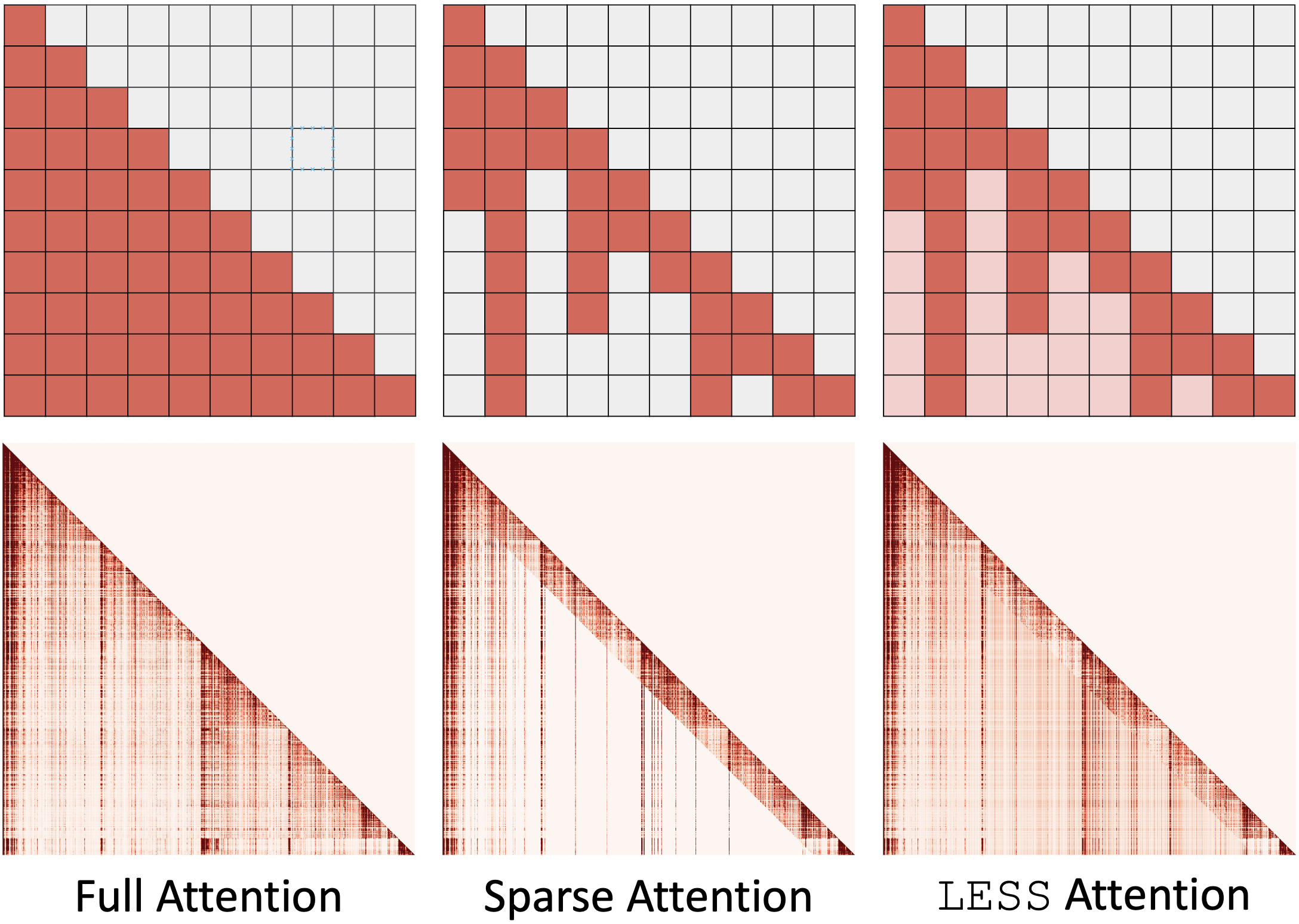
Figure 1: Toy (top row) and Llama 2 7B (bottom row) example decoder attention maps with $\operatorname{\text{H}_{2}\text{O}}$ as the underlying sparse policy. In the top row, red/pink and grey squares are positive and zero attention probabilities, respectively. In the bottom row, darker colors indicate larger attention probabilities. Sparse attention policies zero out many positive attention probabilities. Our method, LESS, ensures all previous tokens will have some contribution to the attention layer output to better retain information.

Thankfully, there have been initiatives to reduce the KV cache size. A line of work, in which we refer to as sparse policies or algorithms, explores the selection of the best subset of KV pairs to cache [ZSZ⁺23, LDL⁺23, HWX⁺23, XTC⁺23]. Although very promising, these methods are inevitably and irrecoverably discarding KV pairs deemed, in one way or another, less important than others, leading to gaps in attention maps

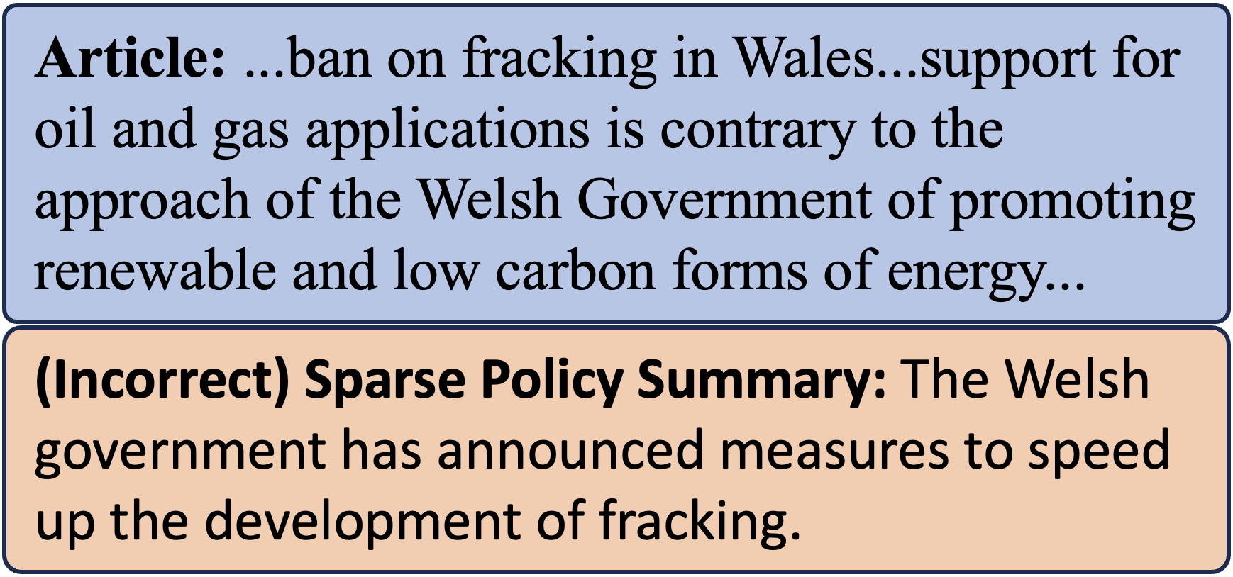
Figure 2: Incorrect summary by Falcon 7B with sparse policy $\operatorname{\text{H}_{2}\text{O}}$.

as shown in Figure 1. Consequently, they are boldly assuming tokens that are unimportant now will not hold significance at future decoding steps, a faulty conjecture for tasks that deviate from this pattern. For instance, using sparse policy $\operatorname{\text{H}_{2}\text{O}}$ [ZSZ⁺23] on Falcon 7B [AAA⁺23] to summarize an article [BBC15, NCL18] produces a factually incorrect summary in Figure 2. For the full article, see Figure 13 in Appendix B.

One way to combat information loss is to cache more tokens, but this is far from memory efficient. An ideal KV cache policy should 1) minimize performance degradation from a full cache, 2) scale at a much slower rate than the full KV cache, and 3) be cheap to integrate into existing pretrained LLMs.

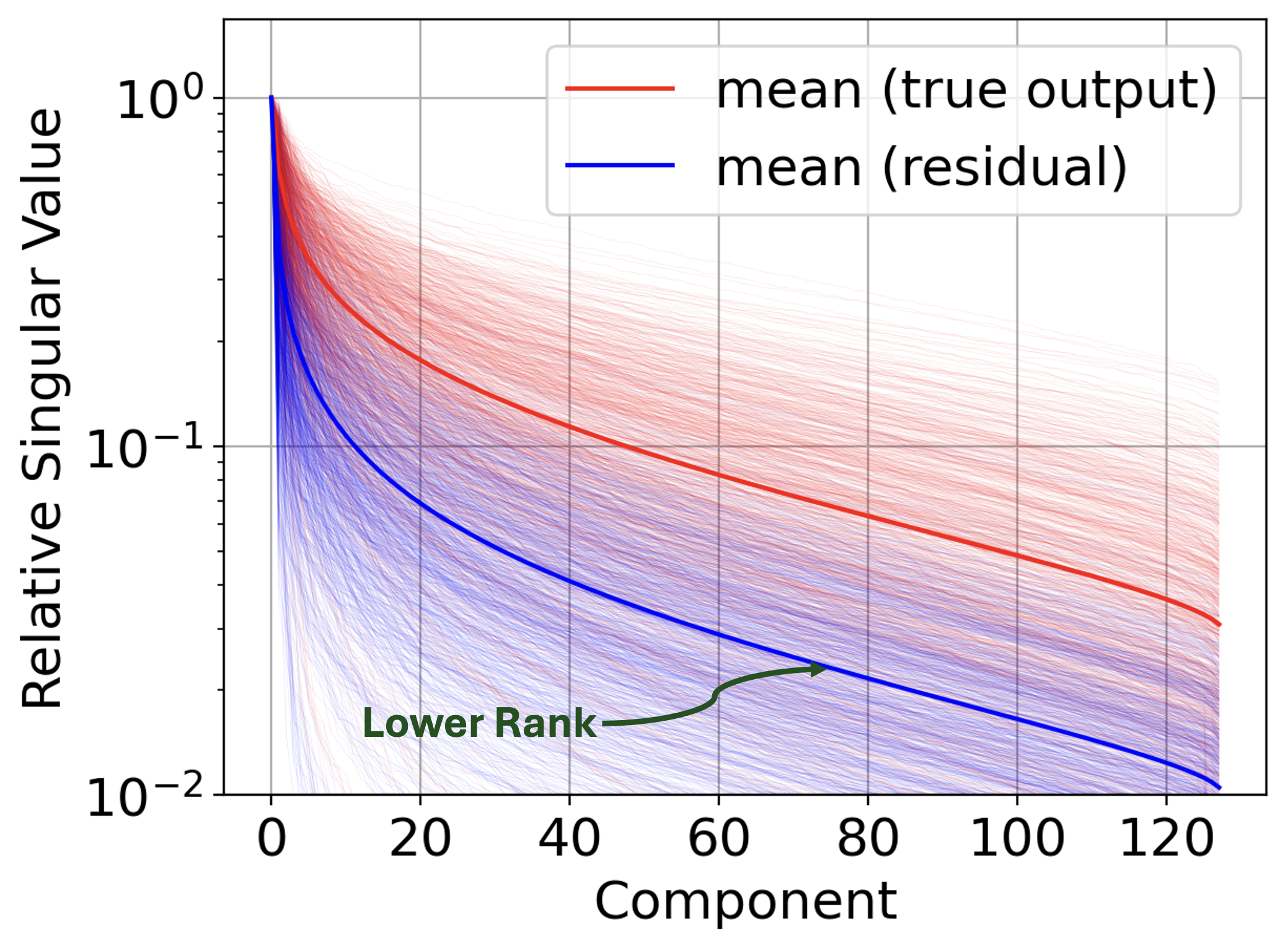
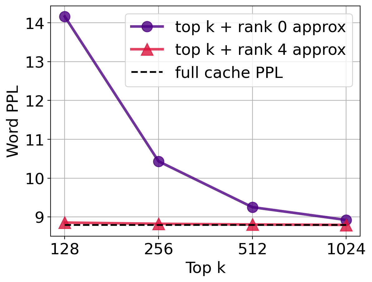
Figure 3: Attention residuals exploration in Llama 2 7B on WikiText [MXBS16]. Mean and 1000 sample relative singular value plots of true attention outputs and residuals from top-$512$ sparse policy, showing the residual is much lower rank (left). End-to-end performance (lower is better) using top-$k$ caching with and without low-rank approximations (right). A rank-4 approximation virtually recovers the original performance.

Fortunately, with some investigation into the residual between full and sparse attention outputs, a better strategy emerges. First, define the residual as $\bm{\Delta}_{\bm{A}}=\bm{A}-\bm{A}_{\text{sparse}}$, where $\bm{A}$ and $\bm{A}_{\text{sparse}}$ are the full and sparse attention outputs, respectively. Using top-$k$ selection as our sparse policy, we observe the residuals $\bm{\Delta}_{\bm{A}}$ are in fact low-rank — more so than $\bm{A}$ — based on Figure 3, a similar observation to Chen et al. [CDW⁺21]. Even a very low-rank approximation can nearly negate the performance degradation from sparse caching. In turn, this finding motivates the use of low-rank methods to approximate the residuals for efficient caches.

We propose LESS (Low-rank Embedding Sidekick with Sparse policy) to learn the residual between the original attention output and the attention output approximated by a sparse policy. LESS does this by accumulating information that would have been discarded by sparse policies into a constant-sized low-rank cache or state, allowing for queries to still access information to recover previously omitted regions in attention maps (see Figure 1).

We show that LESS makes significant progress towards an ideal cache:

1. Performance Improvement: LESS synthesizes sparse KV policies with low-rank states to bridge the performance gap on a variety of tasks where these sparse algorithms show cracks of weakness. In fact, LESS improves the performance much more than simply dedicating that memory to storing more KV pairs.

2. Constant Low-rank Cache Size: Low-rank caches in LESS occupy constant memory with respect to the sequence length, and in our experiments, the extra storage to accommodate LESS is nearly free, taking up the equivalent space of only 4 extra KV pairs in our experiments. Inspired by recurrent networks, the low-rank state stores new information by recursive updates rather than concatenation. As each sample has its own cache, LESS provides the same proportional cache reduction for small and large batch sizes.

3. Cheap Integration: Changes to the LLMs’ architectures are small and do not perturb the original weights. The only modifications to LLMs will be the addition of tiny multilayer perceptions (MLPs) at each attention layer. For example, using LESS with Llama 2 13B adds fewer than 2% of the total number of parameters. In addition, we can train LESS at each attention layer independently from all others, bypassing expensive end-to-end training. Trained once, LESS can transfer to more relaxed settings while maintaining comparable performance, further extending its applicability.

Our comprehensive experiments on Llama 2 [TMS⁺23] and Falcon [AAA⁺23] with different sparse policies [ZSZ⁺23, HWX⁺23, XTC⁺23] on a variety of tasks demonstrates LESS as a highly performative method that reduces KV cache memory. For instance, LESS recovers more than 40% of the Rouge-1 degradation caused by a sparse policy on the CNN/DailyMail dataset [HKG⁺15, SLM17] with Falcon 7B. Finally, we provide an implementation of LESS that reduces the latency by up to $1.3\times$ and increases the throughput by $1.7\times$ from the full cache.

Notation.

We use unbolded letters (e.g. $a,A$), bold lowercase letters (e.g. $\bm{a}$), bold uppercase letters (e.g. $\bm{A}$) for scalars, row vectors, and matrices, respectively. Let $[\bm{A}]_{i,\cdot}$ and $[\bm{A}]_{\cdot,i}$ refer to the $i$-th row and column of $\bm{A}$, respectively. Additionally, define $\bm{0}_{n\times m}$ as a matrix of zeros and $\bm{1}_{n\times m}$ as a matrix of ones, both having shape $n\times m$.

2 Background & Intuition

We start by building the intuition behind LESS. Sparse and low-rank caches individually have noteworthy advantages but also severe drawbacks. Understanding the mechanisms of both (Section 2.1 and 2.2) allows us to effectively synthesize sparse and low-rank structures to create LESS. In Section 2.3, we show that this type of synthesis is a principled approach which has also found success in other areas.

2.1 KV Cache Policies

Many current methods to reduce the KV cache footprint involve keeping a tiny subset of the keys and values either with some pruning policy [LDL⁺23, ZSZ⁺23, HWX⁺23, XTC⁺23, GZL⁺23] or a local attention mechanism [CGRS19, PVU⁺18]. The former method can be applied directly to trained models whereas the latter typically cannot, so with limited compute, deploying a KV cache pruning policy is more practical. Such methods take advantage of the observation that many tokens are irrelevant for attention in some tasks and thus omitting them leads to negligible performance loss. For instance, one of our baselines, $\operatorname{\text{H}_{2}\text{O}}$ [ZSZ⁺23], continuously accumulates attention probabilities at each generation step to identify a set of heavy-hitting tokens to be cached together with the most recent tokens. Not explicitly designed for KV cache compression, algorithms for infinite inference [HWX⁺23, XTC⁺23] maintain a full cache, but as the input sequence exceeds the maximum context length of a model, KV pairs in the middle of the sequence are dropped. Staying within the maximum context length, this results in a cache that maintains the most recent and first few tokens. Regardless of the sparse method, maintaining a tight KV cache budget can seriously impair model performance, as we will see in Section 4.

There also exist promising non-eviction based methods. CacheGen’s KV cache compression at the bit-level takes a query-agnostic approach [LLD⁺23]. In vision tasks, token merging is an effective way to cut down the number of tokens to process [BFD⁺22, RPH⁺22].

2.2 Low-rank Attention

Low-rank structures in attention have been explored extensively [TDBM22], namely from the lens of recurrent neural networks (RNNs). Unlike transformers, RNNs integrate information from all previous tokens into hidden states, analogous low-rank structures to KV caches that organically occupy constant memory. In fact, this feature of RNNs over transformers has motivated research in alternative architectures [DFS⁺22, PMN⁺23, PAA⁺23, SDH⁺23, GD23], but for now, their adoption in LLMs is very limited compared to transformers. Though not as performative as these alternative architectures, linear transformers that break apart the attention operation into kernels also maintain a constant sized KV cache [TBY⁺19, KVPF20, CLD⁺20, PPY⁺21] by reformulating the cache into an RNN hidden state. These types of caching mechanisms are low-rank since information is condensed along the sequence axis, rather than explicitly maintaining individual tokens. This is possible when we replace the softmax with a separable similarity metric $\phi(\bm{q}_{t})\psi(\bm{K}_{t})^{\top}$ for some row-wise functions $\phi$ and $\psi$, letting $\bm{q}_{t}\in\mathbb{R}^{1\times D}$ and $\bm{K}_{t}\in\mathbb{R}^{t\times D}$ be the query and keys at step $t$, respectively. To elaborate, if $\phi$ and $\psi$ are such that

$$\bm{a}_{t}=\text{softmax}\left(\frac{\bm{q}_{t}\bm{K}_{t}^{\top}}{\sqrt{D}}\right)\bm{V}_{t}\approx\frac{\phi(\bm{q}_{t})\psi(\bm{K}_{t})^{\top}\bm{V}_{t}}{\phi(\bm{q}_{t})\psi(\bm{K}_{t})^{\top}\bm{1}_{S\times 1}},$$

we just need to cache hidden states $\bm{H}_{t}=\psi(\bm{K}_{t})^{\top}\bm{V}_{t}\in\mathbb{R}^{R\times D}$ and $\bm{z}_{t}=\sum_{s=1}^{t}\psi([\bm{K}_{t}]_{s})\in\mathbb{R}^{1\times R}$ for inference which can be expressed recursively as

$$\bm{H}_{t+1} =\bm{H}_{t}+\psi(\bm{k}_{t})^{\top}\bm{v}_{t},$$

$$\bm{z}_{t+1} =\bm{z}_{t}+\psi(\bm{k}_{t})$$

for each new KV pair $(\bm{k}_{t},\bm{v}_{t})$. At initialization, $\bm{H}_{0}=\bm{0}_{R\times D}$ and $\bm{z}_{0}=\bm{0}_{1\times R}$. This is a clear improvement from having to store ever increasing sizes of $\bm{K}_{t}$ and $\bm{V}_{t}$, as the memory consumption is independent from $t$. Note that our presentation differs slightly since we do not constrain $\phi=\psi$ [CTTS23]. With this formulation, transformers act like RNNs which occupy constant memory during generation by not appending but updating hidden states during each generation step. Since LLMs are not typically trained in this fashion, a major challenge is to induce this property without significant computation or adjustment to the original weights [KPZ⁺21]. While its dilution of information restricts its performance when specific tokens need to be recalled with strong signals [KHQJ18], this is exactly what a sparse KV cache algorithm can do, so we can fully take advantage of its infinite compression capability to obtain some high level representation of the less important tokens, meaning kernelized attention is a good candidate method for LESS to learn the residual.

2.3 Sparse and Low-rank Decomposition

LESS follows a rich history of decomposing structures into sparse and low-rank components. Particularly, the study of robust principal component analysis [CLMW11, CSPW11] has shown this type of decomposition greatly enhances approximation accuracy and expressibility beyond just sparse or low-rank matrices alone. Its success has spread to deep learning areas such as efficient attention [CDW⁺21], model compression [LYZ⁺23], and fine-tuning [NTA24]. Likewise, we take inspiration from these works in our design.

3 Method

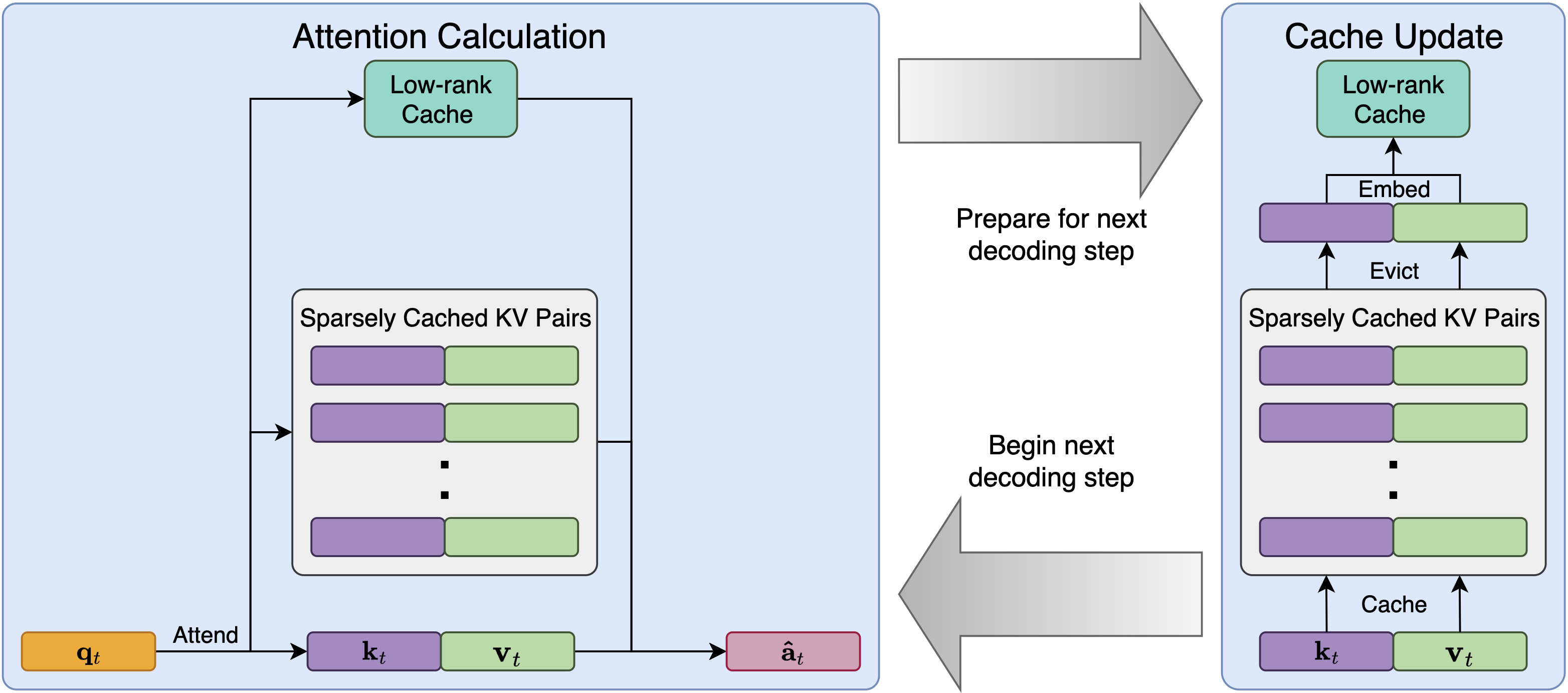
Figure 4: LESS algorithm during inference. At each decoding step, attention is calculated as in (3). To prepare for the next decoding step, the cache is updated by placing the most recent KV pair into the sparse policy cache, and if it has exceeded capacity, a KV pair will be evicted and integrated into the low-rank cache $\bm{H}_{t}$ before being deleted.

When we convert the intuition in Section 2 into an algorithm, a couple technical challenges arise. One challenge is finding an effective way to mix attention probabilities produced by sparse policies and low-rank kernels. Second, we need to design a framework general enough to work with a broad class of sparse policies. In some cases, different sparse policies may be preferable, so our method should be compatible with many sparse policies. Third, our method should be cheap compute to develop. We show that LESS overcomes all these challenges in a two step process: attention computation followed by cache updates.

3.1 KV Caching with LESS

We propose LESS, a general method to synthesize low-rank caches with any eviction-based sparse KV cache policy, $\mathfrak{C}$, to close the performance gap from full KV caching while being efficient. Notably, our method only adds a constant sized cache which does not scale with the sequence length. For the sparse policy, $\mathfrak{C}$, we require that it can output the cached keys $\bm{K}_{\mathfrak{C},t}\in\mathbb{R}^{B_{t}\times D}$, the cached values $\bm{V}_{\mathfrak{C},t}\in\mathbb{R}^{B_{t}\times D}$, and the set of discarded KV pairs $\mathcal{D}_{t}$ at iteration $t$ where $B_{t}\in\mathbb{N}$ is the number of cached pairs.

Letting $\operatorname{\bm{\cdot}}$ denote both $\phi$ and $\psi$, we define our kernels as

$$\phi(\bm{q}) =\left|\sigma_{\phi}(\sigma_{\phi}(\bm{q}\bm{W}_{\phi,1})\bm{W}_{\phi,2})\right|$$ (1)

$$\psi(\bm{k}) =\left|\sigma_{\psi}(\sigma_{\psi}(\bm{k}\bm{W}_{\psi,1})\bm{W}_{\psi,2})\bm{W}_{\psi,3}\right|$$ (2)

for activation functions $\sigma_{\operatorname{\bm{\cdot}}}$, $\bm{W}_{\operatorname{\bm{\cdot}},1}\in\mathbb{R}^{D\times R^{\prime}}$, $\bm{W}_{\operatorname{\bm{\cdot}},2}\in\mathbb{R}^{R^{\prime}\times R}$, and $\bm{W}_{\psi,3}\in\mathbb{R}^{R\times R}$. The element-wise absolute values ensure the inner product $\phi(\bm{q})\psi(\bm{k})^{\top}>0$ to preserve the nonnegativity of attention probabilities. In the ideal case, if $\phi(\bm{q})\psi(\bm{k})^{\top}=e^{\bm{q}\bm{k}^{\top}/\sqrt{D}}$ for all $\bm{q},\bm{k}$, then the result would be the original attention probabilities.

Attention Calculation.

Now, we describe the attention calculation procedure summarized in Algorithm 1. At step $t$, we find the query-key-value triplet $(\bm{q}_{t},\bm{k}_{t},\bm{v}_{t})$ from the input token as usual. Recalling that we have cached $\bm{K}_{\mathfrak{C},t}$, $\bm{V}_{\mathfrak{C},t}$, $\bm{H}_{t}$, and $\bm{z}_{t}$ from the previous generation step, append $\bm{k}_{t}$ to $\bm{K}_{\mathfrak{C},t}$ and $\bm{v}_{t}$ to $\bm{V}_{\mathfrak{C},t}$ to obtain $\bm{K}_{\mathfrak{C},t}^{\prime}\in\mathbb{R}^{(B_{t}+1)\times D}$ and $\bm{V}_{\mathfrak{C},t}^{\prime}\in\mathbb{R}^{(B_{t}+1)\times D}$, respectively. Then, we can find $\hat{\bm{a}}_{t}$, our approximation of the original attention $\bm{a}_{t}$, by computing

$$\hat{\bm{a}}_{t}=\frac{\phi(\bm{q}_{t})\bm{H}_{t}+\exp(\bm{q}_{t}(\bm{K}_{\mathfrak{C},t}^{\prime})^{\top}/\sqrt{D})\bm{V}_{\mathfrak{C},t}^{\prime}}{\phi(\bm{q}_{t})\bm{z}_{t}^{\top}+\exp(\bm{q}_{t}(\bm{K}_{\mathfrak{C},t}^{\prime})^{\top}/\sqrt{D})\bm{1}_{B\times 1}}.$$ (3)

During the prompting phase (i.e. $t=0$), it is just regular attention since $\bm{H}_{0}=\bm{0}_{R\times D}$ and $\bm{z}_{0}=\bm{0}_{1\times R}$.

Cache Updates.

With the attention computed, we need to prepare the necessary ingredients for iteration $t+1$ by finding $\bm{K}_{\mathfrak{C},t+1}$, $\bm{V}_{\mathfrak{C},t+1}$, $\bm{H}_{t+1}$, and $\bm{z}_{t+1}$. The first two are simple since the sparse policy will return $\bm{K}_{\mathfrak{C},t+1}$, $\bm{V}_{\mathfrak{C},t+1}$, and $\mathcal{D}_{t+1}$. Before freeing $\mathcal{D}_{t+1}$ from memory, we embed its information into $\bm{H}_{t+1}$ and $\bm{z}_{t+1}$:

$$\bm{H}_{t+1} =\bm{H}_{t}+\sum_{(\bm{k},\bm{v})\in\mathcal{D}_{t+1}}\psi(\bm{k})^{\top}\bm{v},$$ (4)

$$\bm{z}_{t+1} =\bm{z}_{t}+\sum_{(\bm{k},\bm{v})\in\mathcal{D}_{t+1}}\psi(\bm{k}).$$ (5)

After this, $\mathcal{D}_{t+1}$ can be deleted, and we are prepared for the following generation step. Intuitively, $\bm{H}_{t+1}$ and $\bm{z}_{t+1}$ are updated recursively by keys and values that have been newly pruned at each decoding step. As such, they are constant size repositories of information from all deleted KV pairs which becomes clear when we expand the recursion:

$$\bm{H}_{t+1} =\sum_{(\bm{k},\bm{v})\in\bigcup_{i=1}^{t+1}\mathcal{D}_{i}}\psi(\bm{k})^{\top}\bm{v},$$ (6)

and similarly for $\bm{z}_{t+1}$.

Algorithm 1 Generation Step with LESS

  Input: $\mathfrak{C},\bm{q}_{t},\bm{k}_{t},\bm{v}_{t}$

  Load $\bm{K}_{\mathfrak{C},t},\bm{V}_{\mathfrak{C},t},\bm{H}_{t},\bm{z}_{t}$ from memory.

  $\bm{K}_{\mathfrak{C},t}^{\prime}\leftarrow\text{concatenate}(\bm{K}_{\mathfrak{C},t},\bm{k}_{t})$

  $\bm{V}_{\mathfrak{C},t}^{\prime}\leftarrow\text{concatenate}(\bm{V}_{\mathfrak{C},t},\bm{v}_{t})$

  Obtain $\hat{\bm{a}}_{t}$ via (3).

  Obtain $\bm{K}_{\mathfrak{C},t+1},\bm{V}_{\mathfrak{C},t+1},\mathcal{D}_{t+1}$ from sparse KV cache algorithm $\mathfrak{C}$.

  Update $\bm{H}_{t+1}$ via (4).

  Update $\bm{z}_{t+1}$ via (5).

  Save $\bm{K}_{\mathfrak{C},t+1},\bm{V}_{\mathfrak{C},t+1},\bm{H}_{t+1},\bm{z}_{t+1}$.

  Delete $\mathcal{D}_{t+1}$.

  Return: $\hat{\bm{a}}_{t}$

3.2 Implementation Details

Inexpensive Training.

With our inference-time protocol outlined, we now describe how we can cheaply train our kernel functions $\phi$ and $\psi$. Because training end-to-end is time consuming and resource intensive, we choose to train $\phi$ and $\psi$ at each layer independent of all other layers which already surprisingly gives strong results. The training objective is to minimize the $\ell_{2}$ distance to the output projection of the original attention layer using that layer’s inputs. All weights except for those in $\phi$ and $\psi$ are frozen. As a result, the only computational requirements are the abilities to backpropagate through a single attention layer and run inference on the full model to collect a dataset of attention layer inputs and outputs, which for all models we experiment with, can be done on a single GPU. With more devices, training each layer can be parallelized. While inference follows recursive updates of $\bm{H}_{t}$ and $\bm{z}_{t}$, this does not impede parallelism along the sequence axis because we can just construct the full attention matrix where entries not computed by sparsely cached KV pairs, as determined by whichever sparse policy we train on, will be found by the kernel functions.

All training runs used identical hyperparameters for simplicity. LESS was trained using Adam [KB14] for 40 epochs with an initial learning rate of 0.001 which halved every 10 epochs. We fixed the hidden layer dimension $R^{\prime}=512$, used a dropout rate of 0.3 within the kernels, and let all nonlinear functions $\sigma_{\phi}$ and $\sigma_{\psi}$ to be GELUs. None of the original model’s weights are updated. First, we sampled 512 sequences for Llama 2 models [TMS⁺23] and 1024 sequences for Falcon [AAA⁺23] from the C4 training set [RSR⁺19]. Since Falcon’s context length is half of Llama 2’s, the training sets have the same number of tokens. Next, queries, keys, and values at each layer would be collected as each sample propagated through the models. These collected features (fed in batches of 2) would be used to train the kernels at each layer independently using some sparse policy at some sparsity level. For multi-query attention [Sha19], we extend $\operatorname{\text{H}_{2}\text{O}}$ to aggregate attention scores across all query attention heads to determine KV pairs to evict.

We find that the kernel initialization is critical. As we will show in our experiments (Section 4), the sparse policies already have decent performance which we want to use as a starting point. As such, we add learnable scalars between layers in $\psi$ which are initially set to $10^{-4}$, so the influence of LESS during the first few gradient steps is small. In this way, the sparse policy acts as a warm start, and we can immediately reduce the sparse policy’s residual.

Efficient Generation.

We also develop an implementation that enhances throughput and reduces the latency of LLM generation of LESS. For the sparse cache, we adapt the implementation from Zhang et al. [ZSZ⁺23] to support any KV cache eviction algorithm efficiently. To avoid data movement in memory, we directly replace the evicted KV pair with the newly-added one. As our kernels are small MLPs with GELUs, we implement a fused linear kernel that absorbs the activation into the layer before to avoid writing the intermediate results to DRAM for the low-rank cache.

4 Experiments

Here, we demonstrate the impressive performance of LESS across multiple datasets, models (Llama 2 and Falcon), sparse policies [ZSZ⁺23, HWX⁺23, XTC⁺23], and sparsity levels, despite allocating only approximately 4 tokens of storage to the low-rank state. In Section 4.1, LESS achieves the closest performance to the full cache in language modeling and classification tasks. For example, evaluated with $2\%\operatorname{\text{H}_{2}\text{O}}$ in Llama 2 7B, LESS reduces the word perplexities on WikiText and PG-19 by over 20% from $\operatorname{\text{H}_{2}\text{O}}$ alone, relative to the full cache performance. Section 4.2 shows similar gains in summarization. For example, LESS reduces Rouge-1 degredation by $10\%\operatorname{\text{H}_{2}\text{O}}$ in Falcon 7B on CNN/DailyMail by 41.4%. In Section 4.3, we note the lower latency ($1.1-1.3\times$ reduction) and higher throughput of LESS ($1.7\times$ higher) compared to full caching. Finally, in Section 4.4, we discuss different characteristics of LESS, namely the recovery of true attention probabilities, kernel size scaling, and capabilities for long sequences.

We explore two sparse policies, $\operatorname{\text{H}_{2}\text{O}}$ [ZSZ⁺23] and $\Lambda$-masking from the infinite generation literature [HWX⁺23, XTC⁺23]. When using $\operatorname{\text{H}_{2}\text{O}}$, the sparse KV cache is equally split between the heavy hitter tokens and the recent tokens (e.g. 5% $\operatorname{\text{H}_{2}\text{O}}$ cache consists of 2.5% heavy hitters and 2.5% recent tokens). For $\Lambda$-masking, the cache consists of the first 4 and most recent tokens. The percentages represent how much of the model’s max context length is cached, so regardless of input length, the cache size remains the same for fairness. Since the sparsity level can translate to different numbers of tokens among models based on the max input lengths, we include Table 1 as a quick reference for the models we evaluate on, Llama 2 and Falcon. The token count is rounded down to the nearest even number to make sure $\operatorname{\text{H}_{2}\text{O}}$ can have an even split.

Table 1: Token counts at different sparsity levels.

Model	Max Length	# Tokens at 2%/5%/10%
Llama 2	4096	80 / 204 / 408
Falcon	2048	40 / 102 / 204

For our experiments, we set the kernel size $R=8$, unless otherwise stated. Thus, while minuscule, the size of $\bm{H}$ is nonzero, equivalent to caching 4 extra tokens. We ignore the influence of $\bm{z}$ since it only has $R$ entries. As such, when evaluating on a task at $\alpha$% sparsity, we compare LESS with the sparse policy $\mathfrak{C}$ at $\alpha$% sparsity and at $\alpha$% sparsity plus additional tokens to match the extra space taken by $\bm{H}$ (e.g. 4 tokens in experiments where $R=8$), which we denote as Baseline and Baseline+, respectively. Both are inherently sparse-only policies. A visual representation of the different baselines can be found in Figure 5. Note that the sparsity level and policy $\mathfrak{C}$ will vary throughout our experiments depending on the context. The purpose of evaluating Baseline is to compare the performance gain from extra tokens and the low-rank state $\bm{H}$. Additionally, we evaluate the full KV cache to observe how far we are from the unconstrained potential of the original model. For our method, we denote it as LESS ($\beta$%) where $\beta$ is the percent cache sparsity LESS was trained on with some sparse policy depending on the context.

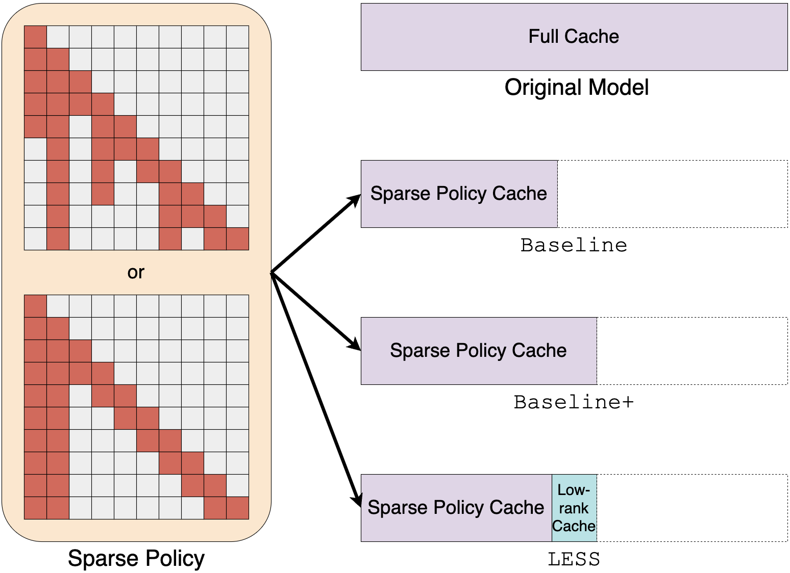
Figure 5: Experimental setup. First, a sparse policy is chosen as the underlying policy behind all methods. Then, we compare performance among the full cache model, Baseline, Baseline+, and LESS. Baseline+ and LESS use the same amount of storage which is slightly larger than the requirements of Baseline.

4.1 Language Modeling & Classification

We start with validating our method trained at different sparsity levels on some language modeling and classification tasks at different sparsity levels using Language Modeling Evaluation Harness [GTA⁺23]. For these tasks, we use the same setup as in training by masking out query-key interactions depending on the sparse policy and having LESS capture the masked probabilities. In addition, we purposefully mismatch training and testing sparsity levels to uncover insight on the transferability between test sparsity levels. To illustrate why a learned kernel is necessary, we also evaluate $\operatorname{\text{H}_{2}\text{O}}$ with Performer kernels [CLD⁺20] based on random Fourier features [RR07], which we denote as $\operatorname{\text{H}_{2}\text{O}}$+Performer.

Table 2 shows Llama 2 7B performance on WikiText [MXBS16] and PG-19 [RPJ⁺19, GBB⁺20] using $\operatorname{\text{H}_{2}\text{O}}$. Looking at the scenarios where training sparsity is equal to the test sparsity, our method is able to achieve much lower word perplexities than the baselines. Notably, LESS beats Baseline by a wider margin than Baseline+ and $\operatorname{\text{H}_{2}\text{O}}$+Performer, indicating that LESS uses the space of 4 extra tokens most effectively. The lackluster performance of $\operatorname{\text{H}_{2}\text{O}}$+Performer suggests that learned kernels are needed to make a noticeable improvement. Moreover, LESS trained at one sparsity level can often generalize reasonably to higher sparsity levels especially on WikiText, even sometimes matching the performance of ones trained at the test sparsity level. The reverse is less effective but can still be better than the baselines. However, all methods are still quite far from the full cache performance.

Table 2: Llama 2 7B WikiText and PG-19 word perplexities with $\operatorname{\text{H}_{2}\text{O}}$ as the primary underlying sparse policy. Numeric column names indicate the sparsity levels during test time. Lower is better.

$\operatorname{\text{H}_{2}\text{O}}$ Method	2% $\operatorname{\text{H}_{2}\text{O}}$	5% $\operatorname{\text{H}_{2}\text{O}}$	10% $\operatorname{\text{H}_{2}\text{O}}$
WikiText
Full Cache	8.791	8.791	8.791
Baseline	13.333	9.863	9.295
Baseline+	12.718	9.842	9.288
$\operatorname{\text{H}_{2}\text{O}}$+Performer	13.332	9.863	9.296
LESS (2%)	10.745	9.658	9.261
LESS (5%)	11.321	9.657	9.239
LESS (10%)	14.577	9.693	9.230
PG-19
Full Cache	23.787	23.787	23.787
Baseline	37.013	27.939	25.451
Baseline+	35.832	27.829	25.429
$\operatorname{\text{H}_{2}\text{O}}$+Performer	36.996	27.938	25.451
LESS (2%)	32.157	27.887	26.322
LESS (5%)	33.195	27.089	25.979
LESS (10%)	41.204	27.201	25.134

Evaluation results [CLC⁺19, CWL⁺20] with $\Lambda$-masking in Table 3 show LESS’s benefit to a different sparse policy (though less performative than $\operatorname{\text{H}_{2}\text{O}}$). Similar to the case with $\operatorname{\text{H}_{2}\text{O}}$, LESS closes the gap from full caching but cannot match the performance completely. While LESS is efficacious for language modeling and classification, we also want to assess its utility for generation where the KV cache storage becomes a critical bottleneck.

Table 3: Llama 2 7B performance on WikiText (word perplexity), MuTual (16-shot R@1), and BoolQ (10-shot accuracy) with 5% $\Lambda$-masking as the primary underlying sparse policy.

$\Lambda$ Method	WikiText ($\downarrow$)	MuTual	BoolQ
Full Cache	8.79	55.08	80.40
Baseline	10.66	53.50	77.28
Baseline+	10.64	53.27	77.46
LESS (5%)	10.12	54.51	78.65

4.2 Summarization

Now, we move on to generation, specifically summarization, to test the ability to generate longer and coherent sequences by synthesizing numerous tokens. Unlike in our language modeling evaluations, the model will have access to all tokens during the prompting phase with the sparse policy and LESS only kicking in during the subsequent generation steps. Consequently, generation sparse policies are fundamentally different from the language modeling masks LESS is trained on, yet despite this, we show that our method maintains its superior performance.

Table 4: Llama 2 13B and Falcon 7B generation quality comparison on CNN/DailyMail and XSum with 408 sparse tokens (10% and 20% of the context lengths of Llama 2 and Falcon, respectively) with $\operatorname{\text{H}_{2}\text{O}}$ as the primary underlying sparse policy. Llama 2 13B is given 5 shots while Falcon 7B is given 3 shots due to its shorter context length. Values are in the format [Rouge-1/2/L].

$\operatorname{\text{H}_{2}\text{O}}$ Method	CNN/DailyMail	XSum
Llama 2 13B
Full Cache	27.55/9.96/25.80	33.14/13.05/27.33
Baseline	23.57/7.35/22.04	33.09/13.09/27.44
Baseline+	23.40/7.31/21.88	33.09/13.06/27.41
LESS (2%)	25.27/7.76/23.64	33.40/12.98/27.41
LESS (5%)	24.45/7.70/22.87	33.15/13.02/27.39
Falcon 7B
Full Cache	25.92/8.52/24.15	27.17/8.83/22.67
Baseline	21.26/5.95/19.73	24.50/7.65/20.50
Baseline+	21.31/6.16/19.75	24.55/7.66/20.56
LESS (5%)	23.00/6.28/21.28	24.94/8.17/20.94
LESS (10%)	23.22/6.37/21.53	25.21/8.28/21.17

Table 5: Llama 2 7B performance on MultiNews (1-shot), CNN/DailyNews (5 shot), and XSum (5-shot) with 5% and 10% $\operatorname{\text{H}_{2}\text{O}}$ as the primary underlying test sparse policies. Values are in the format [Rouge-1]/[Rouge-2]/[Rouge-L].

$\operatorname{\text{H}_{2}\text{O}}$ Method	5% $\operatorname{\text{H}_{2}\text{O}}$	10% $\operatorname{\text{H}_{2}\text{O}}$
MultiNews
Full Cache	23.79/6.87/21.35	23.79/6.87/21.35
Baseline	13.38/3.25/12.25	19.44/4.97/17.73
Baseline+	13.58/3.32/12.41	19.44/4.96/17.72
LESS (2%)	15.31/3.73/14.03	20.32/5.24/18.51
LESS (5%)	15.42/3.80/14.14	20.55/5.29/18.70
CNN/DailyMail
Full Cache	26.25/9.34/24.40	26.25/9.34/24.40
Baseline	18.18/4.92/16.89	20.04/6.09/18.66
Baseline+	18.24/4.91/16.85	20.15/6.21/18.73
LESS (2%)	18.71/5.40/17.34	20.76/6.40/19.32
LESS (5%)	19.21/5.44/17.80	22.29/6.85/20.69
XSum
Full Cache	30.65/11.11/25.40	30.65/11.11/25.40
Baseline	29.03/10.77/24.28	30.68/11.54/25.58
Baseline+	28.94/10.78/24.15	30.64/11.49/25.59
LESS (2%)	30.72/11.53/25.57	30.34/10.98/25.31
LESS (5%)	30.03/11.19/25.03	30.82/11.17/25.56

In Tables 4 and 5, we see LESS achieves better ROUGE [Lin04] scores than purely $\operatorname{\text{H}_{2}\text{O}}$ on the CNN/DailyMail [HKG⁺15, SLM17], MultiNews [FLS⁺19], and XSum [NCL18] datasets. Even at exceptionally low sparsity levels, $\operatorname{\text{H}_{2}\text{O}}$ can capture a significant amount of the full cache’s performance. This is even more surprising for Falcon models which already cache many times fewer tokens than Llama 2 due to the multi-query attention mechanism. Despite this, we observe LESS surpasses the already strong performance of $\operatorname{\text{H}_{2}\text{O}}$ across the board where $\operatorname{\text{H}_{2}\text{O}}$ underperforms compared to the full cache. Like in language modeling, we again see that the improvement from Baseline to Baseline+ pales in comparison to the improvement induced by LESS, sometimes even matching the full cache performance as in XSum. Again, we also see the transferability of LESS to other sparsity levels. See Appendix B for example generation outputs.

4.3 Latency and Throughput

Table 6: Llama 2 7B and 13B’s generation throughput (tokens/s) and latency (s) on an A100 GPU. In the sequence length column, we use "5000 + 5000" to denote a prompt length of 5000 and a generation length of 5000. "OOM" stands for out-of-memory.

Seq. length	Model size	Batch size	Metric	Full Cache	Baseline+	LESS (5%)
5000+5000	13B	4	latency	257.3	185.2	204.7
2048+2048	7B	24	latency	116.7	78.3	95.1
2048+2048	7B	24	throughput	421.2	627.7	516.9
2048+2048	7B	64	throughput	OOM	819.2	699.2

Following Sheng et al. [SZY⁺23], we benchmark the generation throughput and latency of LESS on an NVIDIA A100 80G GPU using FP16 precision. We focus on the Llama 2 7B and 13B models, with all speedup results tested end-to-end with both prompting and generation phases. To measure its performance when generating long sequences or inputting large batch sizes, we use synthetic datasets where all prompts are padded to the same length and batched together. The same number of tokens are generated for each prompt. We test different combinations of prompt and generation lengths.

Table 6 shows results with sequence lengths from 4K to 10K. With the same batch size, LESS reduces the latency by $1.1-1.3\times$ compared to the full cache, though slightly slower than $\operatorname{\text{H}_{2}\text{O}}$. Moreover, LESS saves memory to allow larger batch sizes with a $1.7\times$ improvement on generation throughput for Llama 2 7B, closely matching the performance of $\operatorname{\text{H}_{2}\text{O}}$.

4.4 Empirical Analysis and Ablations

Now that we have shown that LESS is simple and effective, we share some interesting characteristics of our method.

Reconstructing Attention Probabilities.

Sparse KV cache policies can delete tokens that may be needed later on. A way to see this is to construct the sparse attention matrix and compare with the full one. In Figure 1, $\operatorname{\text{H}_{2}\text{O}}$ zeroes out many relatively high attention probabilities with a bias towards keeping early tokens. More examples are in Appendix A. Visually, LESS provides a sketch of the deleted tokens which appears to reasonably reconstruct trends.

Numerically, we measure the similarity of each row in the attention matrix with corresponding rows produced by $\operatorname{\text{H}_{2}\text{O}}$ and LESS with the Hellinger distance, which for two discrete probability vectors, $\bm{p}$ and $\bm{q}$, is defined as

$$\mathcal{H}(\bm{p},\bm{q})\coloneqq\|\sqrt{\bm{p}}-\sqrt{\bm{q}}\|_{2}/\sqrt{2}$$ (7)

where the square root is elementwise. The value of $\mathcal{H}(\bm{p},\bm{q})$ ranges from 0 to 1, where a lower value indicates greater similarity. In Figure 6, we see that our method more accurately replicates the original attention probability distributions as measured by the Hellinger distance. We choose to aggregate each layer separately since the attention distribution patterns tend to vary dramatically throughout the model.

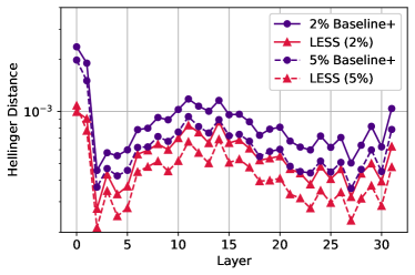
Figure 6: Layer-wise Llama 2 7B mean Hellinger distance from original attention probabilities, aggregated across WikiText evaluation samples. The underlying sparse policy is $\operatorname{\text{H}_{2}\text{O}}$. Here, LESS is evaluated based on their training sparsity percentages.

Larger Kernels.

In our experiments, we fixed $R=8$, and as we show in Figure 7, the performance generally increases as $R$ increases. However, at a certain point, the marginal benefit derived from increasing $R$ is less than shifting more of the KV cache to the sparse policy, suggesting that a small low-rank cache is enough.

Figure 7: Llama 2 7B WikiText word perplexity (lower is better) as the kernel size quadruples, compared against Baseline+ which occupies the same space. The sparse KV cache policy is $\operatorname{\text{H}_{2}\text{O}}$.

Providing Hope for Long Sequences.

Model performance appears to be highly correlated with the input sequence length regardless of the caching method. As shown in Figure 8, even the full cache model performance drops dramatically and immediately as the prompt length increases. Baseline+ and LESS (1% $\operatorname{\text{H}_{2}\text{O}}$) appear to perform similarly for shorter sequences but diverge for longer sequences where we see LESS is more performative. This follows our intuition since for sparse cache policies, a smaller fraction of KV pairs is saved as the sequence length increases, so more information is omitted. This is where a low-rank state can help to recover some of this information.

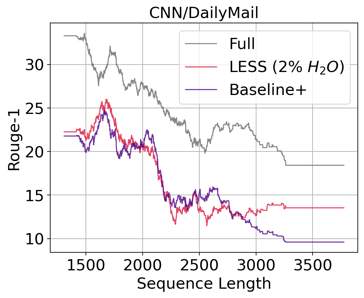
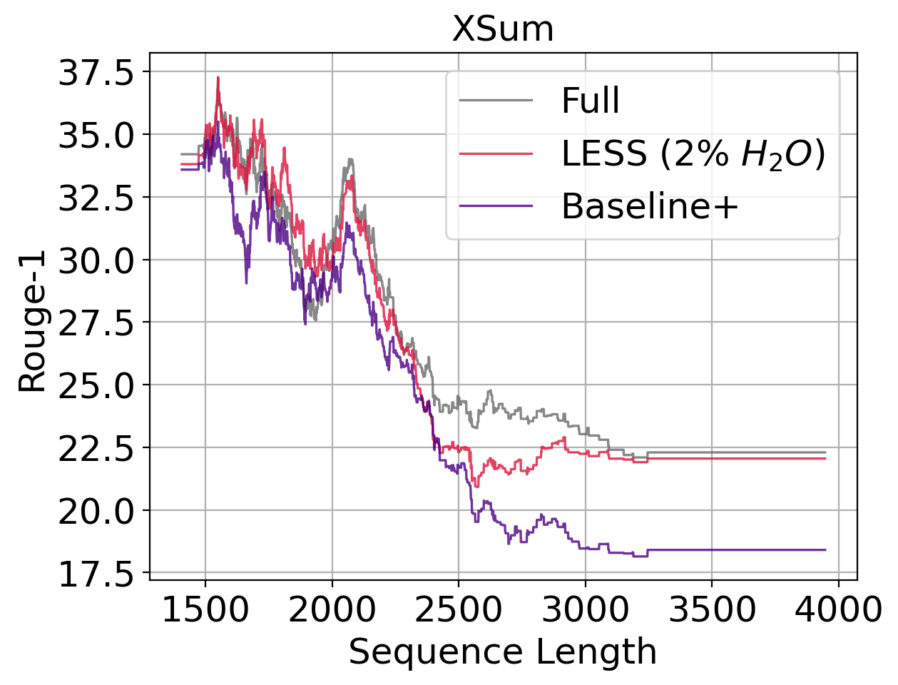
Figure 8: Relationship between Rouge-1 score and prompt length for Llama 2 7B with different cache methods on CNN/DailyMail (left) and XSum (right). The test sparse KV cache policy is 5% $\operatorname{\text{H}_{2}\text{O}}$ for all models. As these results can be fairly noisy, the lines are $k$-nearest regression lines where $k$ is 10% of the dataset size.

5 Conclusion and Future Work

To tackle the KV cache bottleneck, we introduce LESS which has demonstrated itself to be an effective way to boost eviction-based KV cache algorithms. Motivated by the necessity to maintain information that would have been discarded, the constant-sized LESS recovers a significant portion of the performance lost due to maintaining a small cache across a variety of scenarios and intensities, despite being cheap to train and deploy. There are many exciting avenues of work that can enhance LESS or build upon it, such as improving kernel design and investigating the residual of LESS. Such directions will further push the performance of a condensed KV cache to that of a complete cache, allowing LLMs to accomplish the same tasks with less.

Appendix A Attention Matrix Visualizations

This section provides some qualitative results on attention matrix approximations by sparse policies and LESS. While low-rank caches LESS cannot perfectly recover all the missing information, it visually is able to reconstruct a patterns that are completely ignored by sparse policies. We can also see the idiosyncrasies of the sparse policies and LESS, such as $\operatorname{\text{H}_{2}\text{O}}$’s bias towards keeping early tokens, as shown in Figures 9 and 10, and $\Lambda$-masking’s tendency to miss influential tokens which are captured by LESS, as show in Figure 11.

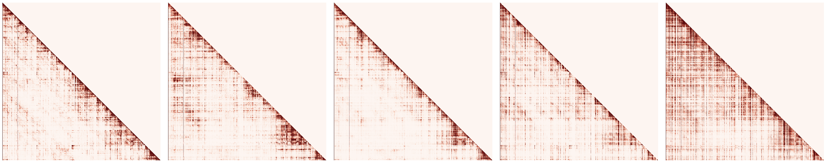
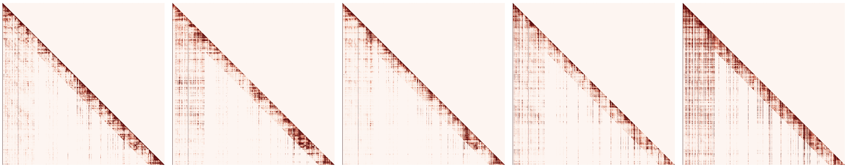
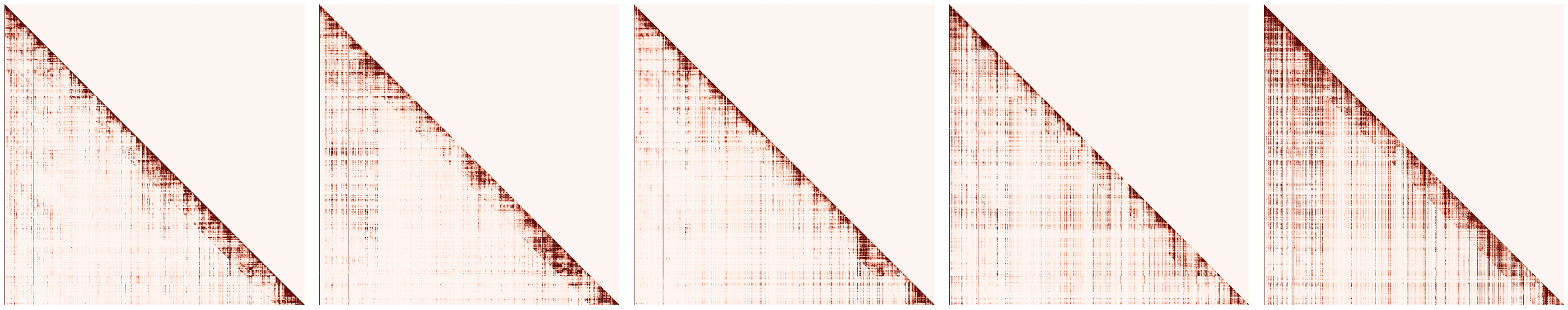
Figure 9: Example attention probability matrices from passing a single input into Falcon 7B. From top to bottom, the rows consist of attention maps from the original model, 10% $\operatorname{\text{H}_{2}\text{O}}$ (204 tokens), and LESS (10% $\operatorname{\text{H}_{2}\text{O}}$). Darker pixels indicate larger probability weights. Only the first 1024 tokens are displayed.

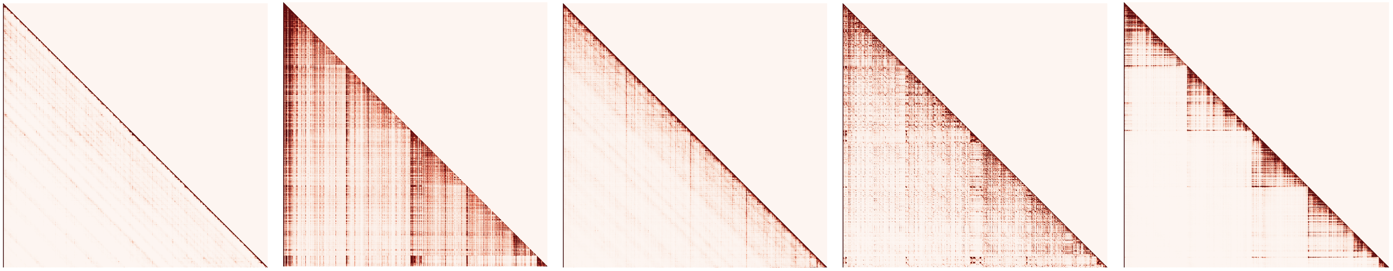
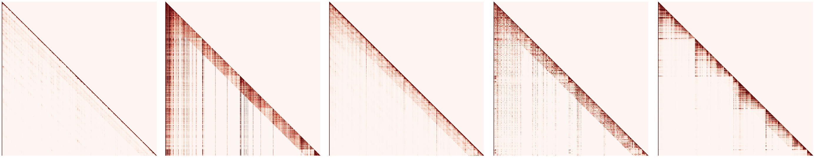
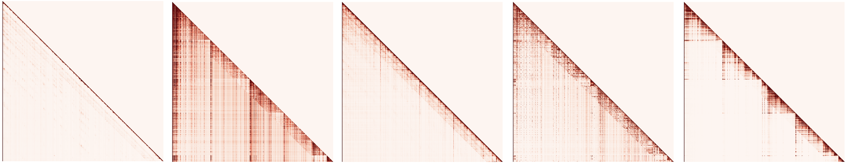
Figure 10: Example attention probability matrices from passing a single input into Llama 2 7B. From top to bottom, the rows consist of attention maps from the original model, 5% $\operatorname{\text{H}_{2}\text{O}}$ (204 tokens), and LESS (5% $\operatorname{\text{H}_{2}\text{O}}$). Darker pixels indicate larger probability weights. Only the first 1024 tokens are displayed.

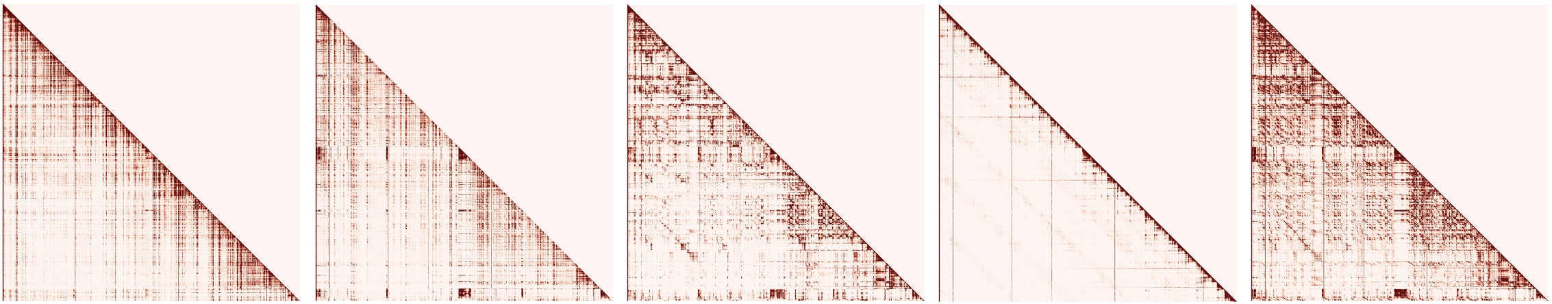
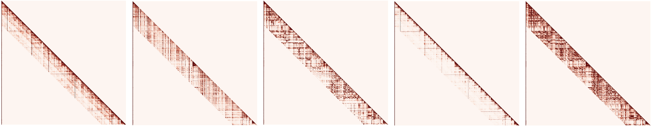
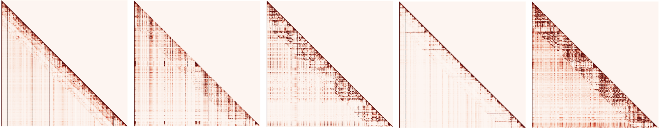
Figure 11: Example attention probability matrices from passing a single input into Llama 2 7B. From top to bottom, the rows consist of attention maps from the original model, 5% $\Lambda$-masking (204 tokens), and LESS (5% $\Lambda$). Darker pixels indicate larger probability weights. Only the first 1024 tokens are displayed.

Appendix B Generation Outputs

We include a couple examples of generation outputs in Figure 12 and Figure 13. In both cases, the full cache, LESS, and Baseline+ models attempt to summarize news articles. We see in Figure 12 that LESS is able to produce the same concise summary as the full cache while Baseline+ produces rambling text. In Figure 13, we observe that LESS completely changes the meaning of the summary from $\operatorname{\text{H}_{2}\text{O}}$ alone–Baseline+ is factually incorrect based on the article.

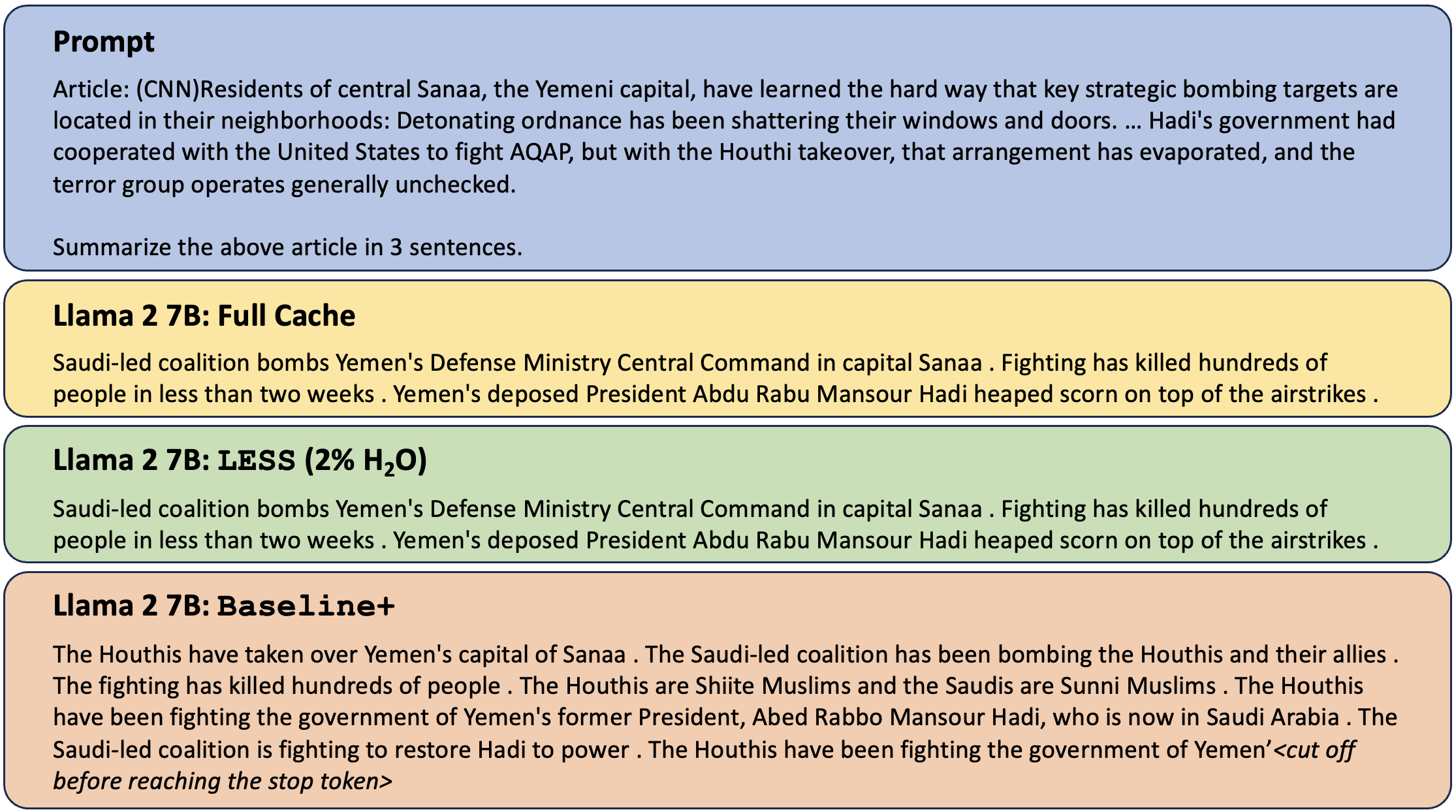
Figure 12: Example 5-shot (not shown) CNN/DailyMail summary generation results produced by variations of Llama 2 7B with an underlying sparse policy of 2% $\operatorname{\text{H}_{2}\text{O}}$. For brevity, only the start and end of the article are shown with the middle omitted with an ellipsis. LESS produces the same concise summary as the full cache while Baseline+ produces rambling text, exceeding the 3 sentence requirement by the prompt. The original article is from [Bru15].

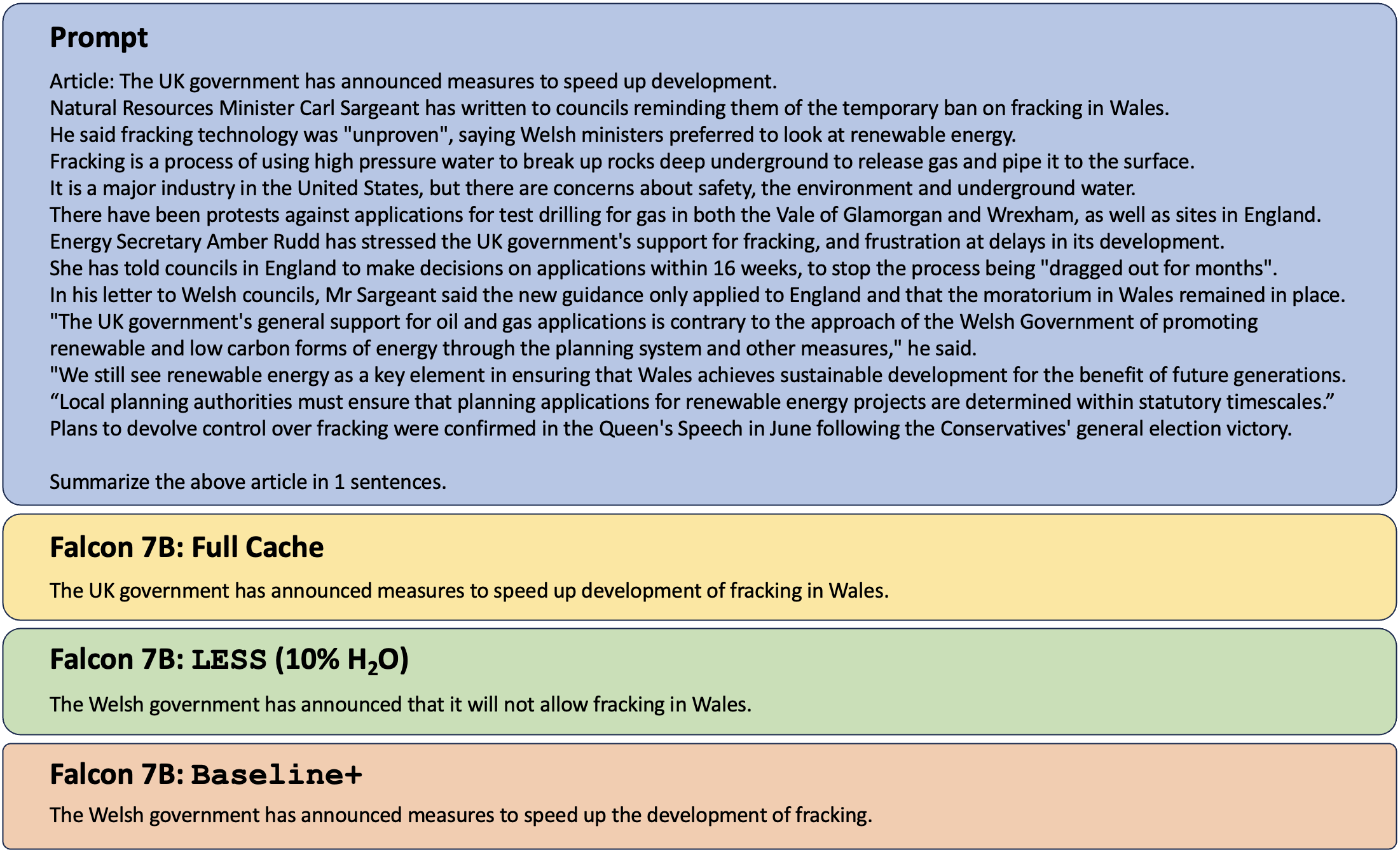
Figure 13: Example 3-shot (not shown) XSum summary generation results produced by variations of Falcon 7B. Models were evaluated with 20% $\operatorname{\text{H}_{2}\text{O}}$. The summary by Baseline+ is factually incorrect based on the article, while LESS preserves the meaning better. The original article is from [BBC15].

References

- [AAA+23] E. Almazrouei, H. Alobeidli, A. Alshamsi, A. Cappelli, R. Cojocaru, M. Debbah, E. Goffinet, D. Heslow, J. Launay, Q. Malartic, B. Noune, B. Pannier, and G. Penedo. Falcon-40B: an open large language model with state-of-the-art performance. 2023.
- [ADF+23] R. Anil, A. M. Dai, O. Firat, M. Johnson, D. Lepikhin, A. Passos, S. Shakeri, E. Taropa, P. Bailey, Z. Chen, et al. Palm 2 technical report. arXiv preprint arXiv:2305.10403, 2023.
- [BBC15] BBC. Fracking still opposed in wales, ministers tell councils. The British Broadcasting Corporation, 2015.
- [BFD+22] D. Bolya, C.-Y. Fu, X. Dai, P. Zhang, C. Feichtenhofer, and J. Hoffman. Token merging: Your vit but faster. arXiv preprint arXiv:2210.09461, 2022.
- [Bru15] B. Brumfield. Death toll rises quickly as conflict rages in yemen. The Cable News Network, 2015.
- [CDW+21] B. Chen, T. Dao, E. Winsor, Z. Song, A. Rudra, and C. Ré. Scatterbrain: Unifying sparse and low-rank attention. Advances in Neural Information Processing Systems, 34:17413–17426, 2021.
- [CGRS19] R. Child, S. Gray, A. Radford, and I. Sutskever. Generating long sequences with sparse transformers. arXiv preprint arXiv:1904.10509, 2019.
- [CLC+19] C. Clark, K. Lee, M.-W. Chang, T. Kwiatkowski, M. Collins, and K. Toutanova. Boolq: Exploring the surprising difficulty of natural yes/no questions. arXiv preprint arXiv:1905.10044, 2019.
- [CLD+20] K. Choromanski, V. Likhosherstov, D. Dohan, X. Song, A. Gane, T. Sarlos, P. Hawkins, J. Davis, A. Mohiuddin, L. Kaiser, et al. Rethinking attention with performers. arXiv preprint arXiv:2009.14794, 2020.
- [CLMW11] E. J. Candès, X. Li, Y. Ma, and J. Wright. Robust principal component analysis? Journal of the ACM (JACM), 58(3):1–37, 2011.
- [CSPW11] V. Chandrasekaran, S. Sanghavi, P. A. Parrilo, and A. S. Willsky. Rank-sparsity incoherence for matrix decomposition. SIAM Journal on Optimization, 21(2):572–596, 2011.
- [CTTS23] Y. Chen, Q. Tao, F. Tonin, and J. A. Suykens. Primal-attention: Self-attention through asymmetric kernel svd in primal representation. arXiv preprint arXiv:2305.19798, 2023.
- [CWL+20] L. Cui, Y. Wu, S. Liu, Y. Zhang, and M. Zhou. Mutual: A dataset for multi-turn dialogue reasoning. arXiv preprint arXiv:2004.04494, 2020.
- [DFS+22] T. Dao, D. Y. Fu, K. K. Saab, A. W. Thomas, A. Rudra, and C. Ré. Hungry hungry hippos: Towards language modeling with state space models. arXiv preprint arXiv:2212.14052, 2022.
- [FLS+19] A. R. Fabbri, I. Li, T. She, S. Li, and D. R. Radev. Multi-news: a large-scale multi-document summarization dataset and abstractive hierarchical model, 2019.
- [FZS22] W. Fedus, B. Zoph, and N. Shazeer. Switch transformers: Scaling to trillion parameter models with simple and efficient sparsity. The Journal of Machine Learning Research, 23(1):5232–5270, 2022.
- [GBB+20] L. Gao, S. Biderman, S. Black, L. Golding, T. Hoppe, C. Foster, J. Phang, H. He, A. Thite, N. Nabeshima, et al. The pile: An 800gb dataset of diverse text for language modeling. arXiv preprint arXiv:2101.00027, 2020.
- [GD23] A. Gu and T. Dao. Mamba: Linear-time sequence modeling with selective state spaces. arXiv preprint arXiv:2312.00752, 2023.
- [GTA+23] L. Gao, J. Tow, B. Abbasi, S. Biderman, S. Black, A. DiPofi, C. Foster, L. Golding, J. Hsu, A. Le Noac’h, H. Li, K. McDonell, N. Muennighoff, C. Ociepa, J. Phang, L. Reynolds, H. Schoelkopf, A. Skowron, L. Sutawika, E. Tang, A. Thite, B. Wang, K. Wang, and A. Zou. A framework for few-shot language model evaluation, 12 2023.
- [GZL+23] S. Ge, Y. Zhang, L. Liu, M. Zhang, J. Han, and J. Gao. Model tells you what to discard: Adaptive kv cache compression for llms. arXiv preprint arXiv:2310.01801, 2023.
- [HKG+15] K. M. Hermann, T. KociskÃœ, E. Grefenstette, L. Espeholt, W. Kay, M. Suleyman, and P. Blunsom. Teaching machines to read and comprehend. In NIPS, pages 1693–1701, 2015.
- [HWX+23] C. Han, Q. Wang, W. Xiong, Y. Chen, H. Ji, and S. Wang. Lm-infinite: Simple on-the-fly length generalization for large language models. arXiv preprint arXiv:2308.16137, 2023.
- [JSR+24] A. Q. Jiang, A. Sablayrolles, A. Roux, A. Mensch, B. Savary, C. Bamford, D. S. Chaplot, D. de las Casas, E. B. Hanna, F. Bressand, G. Lengyel, G. Bour, G. Lample, L. R. Lavaud, L. Saulnier, M.-A. Lachaux, P. Stock, S. Subramanian, S. Yang, S. Antoniak, T. L. Scao, T. Gervet, T. Lavril, T. Wang, T. Lacroix, and W. E. Sayed. Mixtral of experts, 2024.
- [KB14] D. P. Kingma and J. Ba. Adam: A method for stochastic optimization. arXiv preprint arXiv:1412.6980, 2014.
- [KHQJ18] U. Khandelwal, H. He, P. Qi, and D. Jurafsky. Sharp nearby, fuzzy far away: How neural language models use context. arXiv preprint arXiv:1805.04623, 2018.
- [KNH+22] S. Khan, M. Naseer, M. Hayat, S. W. Zamir, F. S. Khan, and M. Shah. Transformers in vision: A survey. ACM computing surveys (CSUR), 54(10s):1–41, 2022.
- [KPZ+21] J. Kasai, H. Peng, Y. Zhang, D. Yogatama, G. Ilharco, N. Pappas, Y. Mao, W. Chen, and N. A. Smith. Finetuning pretrained transformers into rnns. arXiv preprint arXiv:2103.13076, 2021.
- [KVPF20] A. Katharopoulos, A. Vyas, N. Pappas, and F. Fleuret. Transformers are rnns: Fast autoregressive transformers with linear attention. In International conference on machine learning, pages 5156–5165. PMLR, 2020.
- [LDL+23] Z. Liu, A. Desai, F. Liao, W. Wang, V. Xie, Z. Xu, A. Kyrillidis, and A. Shrivastava. Scissorhands: Exploiting the persistence of importance hypothesis for llm kv cache compression at test time. arXiv preprint arXiv:2305.17118, 2023.
- [Lin04] C.-Y. Lin. ROUGE: A package for automatic evaluation of summaries. In Text Summarization Branches Out, pages 74–81, Barcelona, Spain, July 2004. Association for Computational Linguistics.
- [LLD+23] Y. Liu, H. Li, K. Du, J. Yao, Y. Cheng, Y. Huang, S. Lu, M. Maire, H. Hoffmann, A. Holtzman, et al. Cachegen: Fast context loading for language model applications. arXiv preprint arXiv:2310.07240, 2023.
- [LWLQ22] T. Lin, Y. Wang, X. Liu, and X. Qiu. A survey of transformers. AI Open, 2022.
- [LYZ+23] Y. Li, Y. Yu, Q. Zhang, C. Liang, P. He, W. Chen, and T. Zhao. Losparse: Structured compression of large language models based on low-rank and sparse approximation. arXiv preprint arXiv:2306.11222, 2023.
- [MXBS16] S. Merity, C. Xiong, J. Bradbury, and R. Socher. Pointer sentinel mixture models, 2016.
- [NBZ+23] S. Nerella, S. Bandyopadhyay, J. Zhang, M. Contreras, S. Siegel, A. Bumin, B. Silva, J. Sena, B. Shickel, A. Bihorac, et al. Transformers in healthcare: A survey. arXiv preprint arXiv:2307.00067, 2023.
- [NCL18] S. Narayan, S. B. Cohen, and M. Lapata. Don’t give me the details, just the summary! topic-aware convolutional neural networks for extreme summarization. arXiv preprint arXiv:1808.08745, 2018.
- [NTA24] M. Nikdan, S. Tabesh, and D. Alistarh. Rosa: Accurate parameter-efficient fine-tuning via robust adaptation. arXiv preprint arXiv:2401.04679, 2024.
- [PAA+23] B. Peng, E. Alcaide, Q. Anthony, A. Albalak, S. Arcadinho, H. Cao, X. Cheng, M. Chung, M. Grella, K. K. GV, et al. Rwkv: Reinventing rnns for the transformer era. arXiv preprint arXiv:2305.13048, 2023.
- [PDC+23] R. Pope, S. Douglas, A. Chowdhery, J. Devlin, J. Bradbury, J. Heek, K. Xiao, S. Agrawal, and J. Dean. Efficiently scaling transformer inference. Proceedings of Machine Learning and Systems, 5, 2023.
- [PMN+23] M. Poli, S. Massaroli, E. Nguyen, D. Y. Fu, T. Dao, S. Baccus, Y. Bengio, S. Ermon, and C. Ré. Hyena hierarchy: Towards larger convolutional language models. arXiv preprint arXiv:2302.10866, 2023.
- [PPY+21] H. Peng, N. Pappas, D. Yogatama, R. Schwartz, N. A. Smith, and L. Kong. Random feature attention. arXiv preprint arXiv:2103.02143, 2021.
- [PVU+18] N. Parmar, A. Vaswani, J. Uszkoreit, L. Kaiser, N. Shazeer, A. Ku, and D. Tran. Image transformer. In International conference on machine learning, pages 4055–4064. PMLR, 2018.
- [RPH+22] C. Renggli, A. S. Pinto, N. Houlsby, B. Mustafa, J. Puigcerver, and C. Riquelme. Learning to merge tokens in vision transformers. arXiv preprint arXiv:2202.12015, 2022.
- [RPJ+19] J. W. Rae, A. Potapenko, S. M. Jayakumar, C. Hillier, and T. P. Lillicrap. Compressive transformers for long-range sequence modelling. arXiv preprint, 2019.
- [RR07] A. Rahimi and B. Recht. Random features for large-scale kernel machines. Advances in neural information processing systems, 20, 2007.
- [RSR+19] C. Raffel, N. Shazeer, A. Roberts, K. Lee, S. Narang, M. Matena, Y. Zhou, W. Li, and P. J. Liu. Exploring the limits of transfer learning with a unified text-to-text transformer. arXiv e-prints, 2019.
- [SDH+23] Y. Sun, L. Dong, S. Huang, S. Ma, Y. Xia, J. Xue, J. Wang, and F. Wei. Retentive network: A successor to transformer for large language models. arXiv preprint arXiv:2307.08621, 2023.
- [SFA+22] T. L. Scao, A. Fan, C. Akiki, E. Pavlick, S. Ilić, D. Hesslow, R. Castagné, A. S. Luccioni, F. Yvon, M. Gallé, et al. Bloom: A 176b-parameter open-access multilingual language model. arXiv preprint arXiv:2211.05100, 2022.
- [Sha19] N. Shazeer. Fast transformer decoding: One write-head is all you need. arXiv preprint arXiv:1911.02150, 2019.
- [SLM17] A. See, P. J. Liu, and C. D. Manning. Get to the point: Summarization with pointer-generator networks. In Proceedings of the 55th Annual Meeting of the Association for Computational Linguistics (Volume 1: Long Papers), pages 1073–1083, Vancouver, Canada, July 2017. Association for Computational Linguistics.
- [SZY+23] Y. Sheng, L. Zheng, B. Yuan, Z. Li, M. Ryabinin, D. Y. Fu, Z. Xie, B. Chen, C. W. Barrett, J. Gonzalez, P. Liang, C. Ré, I. Stoica, and C. Zhang. High-throughput generative inference of large language models with a single gpu. In International Conference on Machine Learning, 2023.
- [TAB+23] G. Team, R. Anil, S. Borgeaud, Y. Wu, J.-B. Alayrac, J. Yu, R. Soricut, J. Schalkwyk, A. M. Dai, A. Hauth, et al. Gemini: a family of highly capable multimodal models. arXiv preprint arXiv:2312.11805, 2023.
- [TBY+19] Y.-H. H. Tsai, S. Bai, M. Yamada, L.-P. Morency, and R. Salakhutdinov. Transformer dissection: a unified understanding of transformer’s attention via the lens of kernel. arXiv preprint arXiv:1908.11775, 2019.
- [TDBM22] Y. Tay, M. Dehghani, D. Bahri, and D. Metzler. Efficient transformers: A survey, 2022.
- [TMS+23] H. Touvron, L. Martin, K. Stone, P. Albert, A. Almahairi, Y. Babaei, N. Bashlykov, S. Batra, P. Bhargava, S. Bhosale, et al. Llama 2: Open foundation and fine-tuned chat models. arXiv preprint arXiv:2307.09288, 2023.
- [VSP+17] A. Vaswani, N. Shazeer, N. Parmar, J. Uszkoreit, L. Jones, A. N. Gomez, Ł. Kaiser, and I. Polosukhin. Attention is all you need. Advances in neural information processing systems, 30, 2017.
- [XTC+23] G. Xiao, Y. Tian, B. Chen, S. Han, and M. Lewis. Efficient streaming language models with attention sinks. arXiv preprint arXiv:2309.17453, 2023.
- [ZRG+22] S. Zhang, S. Roller, N. Goyal, M. Artetxe, M. Chen, S. Chen, C. Dewan, M. Diab, X. Li, X. V. Lin, T. Mihaylov, M. Ott, S. Shleifer, K. Shuster, D. Simig, P. S. Koura, A. Sridhar, T. Wang, and L. Zettlemoyer. Opt: Open pre-trained transformer language models, 2022.
- [ZSZ+23] Z. Zhang, Y. Sheng, T. Zhou, T. Chen, L. Zheng, R. Cai, Z. Song, Y. Tian, C. Ré, C. Barrett, et al. H o: Heavy-hitter oracle for efficient generative inference of large language models. arXiv preprint arXiv:2306.14048, 2023.