Fixed-sparsity matrix approximation from
matrix-vector products

Abstract

We study the problem of approximating a matrix $\mathbf{A}$ with a matrix that has a fixed sparsity pattern (e.g., diagonal, banded, etc.), when $\mathbf{A}$ is accessed only by matrix-vector products. We describe a simple randomized algorithm that returns an approximation with the given sparsity pattern with Frobenius-norm error at most $(1+\varepsilon)$ times the best possible error. When each row of the desired sparsity pattern has at most $s$ nonzero entries, this algorithm requires $O(s/\varepsilon)$ non-adaptive matrix-vector products with $\mathbf{A}$. We also prove a matching lower-bound, showing that, for any sparsity pattern with $\Theta(s)$ nonzeros per row and column, any algorithm achieving $(1+\epsilon)$ approximation requires $\Omega(s/\varepsilon)$ matrix-vector products in the worst case. We thus resolve the matrix-vector product query complexity of the problem up to constant factors, even for the well-studied case of diagonal approximation, for which no previous lower bounds were known.

1 Introduction

Learning about a matrix $\mathbf{A}$ from matrix-vector product (matvec) queries $\mathbf{x}_{1},\ldots,\mathbf{x}_{m}\mapsto\mathbf{A}\mathbf{x}_{1},\ldots,\mathbf{A}\mathbf{x}_{m}$ is a widespread task in numerical linear algebra, theoretical computer science, and machine learning. Algorithms that only access $\mathbf{A}$ through matvec queries (also known as matrix-free algorithms) are useful when $\mathbf{A}$ is not known explicitly, but admits efficient matvecs. Common settings include when $\mathbf{A}$ is a solution operator for a linear partial differential equation [Kar+21, SO21, BET22], a function of another matrix that can be applied with Krylov subspace methods [GS92, Hig08], the Hessian of a neural network that can be applied via back-propagation [Pea94], or a data matrix in compressed sensing applications [KK11]. Matrix-free algorithms are often the methods of choice due to practical considerations such as memory usage and data movement. If the queries are chosen non-adaptively — i.e, the $i$-th query vector $\mathbf{x}_{i}$ does not depend on the results $\mathbf{Ax}_{1},\ldots,\mathbf{Ax}_{i-1}$ from previous queries — queries can be parallelized, potentially leading to substantial runtime improvements [Mur+23]. Non-adaptive queries can also be computed in a single pass over $\mathbf{A}$, and thus, non-adaptive matvec query algorithms are an important tool in streaming and distributed computation [CW09, MT20].

In many cases, the cost of matrix-free algorithms is dominated by the cost of the matvec queries. As such, a key goal is to understand the minimum number of queries required to solve a given problem, also known as the query complexity. Any algorithm automatically yields an upper bound on the query complexity, whereas it can be more challenging to prove lower bounds. Problems for which the matvec query complexity have been extensively studied include low-rank approximation [HMT11, SER18, TW23, BCW22, BN23, HT23], spectrum approximation [Ski89, WWAF06, SW23], trace and diagonal estimation [Gir87, Hut89, BKS07, MMMW21], the approximation of linear system solutions and the action of matrix functions [GS92, Gre97, BHSW20], and matrix property testing [SWYZ21, NSW22].

An important class of problems considers recovering $\mathbf{A}$ from matvec queries when $\mathbf{A}$ is structured, or relatedly, finding the nearest approximation to $\mathbf{A}$ within a structured class of matrices. Example classes that have been studied extensively in this setting include low-rank matrices [HMT11, TW23], hierarchical low-rank matrices [LLY11, Mar16, LM22, LM22a, SO21, HT23], diagonal matrices [BKS07, TS11, BN22, DM23], sparse matrices [CPR74, CM83, CC86, WEV13, DSBN15], and beyond [WSB11, SKO21].

1.1 Fixed-sparsity matrix approximation

In this work, we focus on the task of approximating $\mathbf{A}$ with a matrix of a specified sparsity pattern, with error competitive with the best approximation of the given sparsity pattern. This is a natural task; indeed, there are many existing linear algebra algorithms for matrices of a given sparsity pattern (e.g. diagonal, tridiagonal, banded, block diagonal, etc.), so it is a common goal to obtain an approximation compatible with such algorithms. As we discuss in Section 1.3, several important special cases including diagonal approximation and exact recovery of matrices with known-sparsity have been studied extensively in prior work.

Formally, using “$\,\circ\,$” to indicate the Hadamard (entrywise) product and $\|\cdot\|_{\mathsf{F}}$ to denote the Frobenius norm, we consider the following problem:

Problem 1 (Best approximation by a matrix of fixed sparsity).

Given a matrix $\mathbf{A}\in\mathbb{R}^{n\times d}$ and a binary matrix $\mathbf{S}\in\{0,1\}^{n\times d}$, find a matrix $\widetilde{\mathbf{A}}$ so that $\widetilde{\mathbf{A}}=\mathbf{S}\circ\widetilde{\mathbf{A}}$ and

$$\|\mathbf{A}-\widetilde{\mathbf{A}}\|_{\mathsf{F}}\leq(1+\varepsilon)\,\|\mathbf{A}-\mathbf{S}\circ\mathbf{A}\|_{\mathsf{F}}.$$

Observe that $\mathbf{S}\circ\mathbf{A}$ is the matrix of sparsity $\mathbf{S}$ nearest to $\mathbf{A}$ in the Frobenius norm:

$$\mathbf{S}\circ\mathbf{A}=\operatornamewithlimits{argmin}_{\mathbf{X}=\mathbf{S}\circ\mathbf{X}}\|\mathbf{A}-\mathbf{X}\|_{\mathsf{F}}.$$

Hence, Problem 1 is asking for a near-optimal approximation to $\mathbf{A}$ of the given sparsity $\mathbf{S}$. In particular, if $\mathbf{A}$ already has sparsity pattern $\mathbf{S}$, then $\mathbf{A}=\mathbf{S}\circ\mathbf{A}$, so solving Problem 1 will recover $\mathbf{A}$ exactly.

In addressing Problem 1, it will also be beneficial to consider the closely related problem of recovering the “sparse-part” of a matrix:

Problem 2 (Best approximation to on-sparsity-pattern entries).

Given a matrix $\mathbf{A}\in\mathbb{R}^{n\times d}$ and a binary matrix $\mathbf{S}\in\{0,1\}^{n\times d}$, find a matrix $\widetilde{\mathbf{A}}$ so that $\widetilde{\mathbf{A}}=\mathbf{S}\circ\widetilde{\mathbf{A}}$ and

$$\|\mathbf{S}\circ\mathbf{A}-\widetilde{\mathbf{A}}\|_{\mathsf{F}}^{2}\leq\varepsilon\,\|\mathbf{A}-\mathbf{S}\circ\mathbf{A}\|_{\mathsf{F}}^{2}.$$

Note the presence of the squared norms in Problem 2. Since $\widetilde{\mathbf{A}}$ has the same sparsity as $\mathbf{S}$; i.e. $\widetilde{\mathbf{A}}=\mathbf{S}\circ\widetilde{\mathbf{A}}$,

$$\|\mathbf{A}-\widetilde{\mathbf{A}}\|_{\mathsf{F}}^{2}=\|\mathbf{A}-\mathbf{S}\circ\mathbf{A}\|_{\mathsf{F}}^{2}+\|\mathbf{S}\circ\mathbf{A}-\widetilde{\mathbf{A}}\|_{\mathsf{F}}^{2}.$$ (1)

Thus, using the fact that $\sqrt{1+2\varepsilon}<1+\varepsilon$ for all $\varepsilon>0$, a solution to Problem 2 with accuracy ${2\varepsilon}$ immediately yields a solution to Problem 1 with accuracy $\varepsilon$. Conversely, if $\varepsilon\in(0,1)$ so that $\sqrt{1+3\varepsilon}\geq 1+\varepsilon$, then a solution to Problem 1 with accuracy $\varepsilon$ yields a solution to Problem 2 with accuracy ${3\varepsilon}$. In this sense, the problems are equivalent.

1.2 Our Contributions and Roadmap

Our first contribution is to analyze a simple algorithm (Algorithm 1) that solves Problems 1 and 2. When the sparsity pattern $\mathbf{S}$ has at most $s$ non-zero entries per row, this algorithm uses $m=O(s/\varepsilon)$ non-adaptive matrix-vector product queries. Specifically, the algorithm computes $\mathbf{Z}=\mathbf{A}\mathbf{G}$, where $\mathbf{G}$ is a $d\times m$ matrix with independent standard normal entries, and then outputs the matrix

$$\widetilde{\mathbf{A}}=\operatornamewithlimits{argmin}_{\mathbf{X}=\mathbf{S}\circ\mathbf{X}}\|\mathbf{Z}-\mathbf{X}\mathbf{G}\|_{\mathsf{F}}.$$ (2)

We make no claims about the novelty of the algorithm, which follows immediately from ideas in compressed sensing. In Section 2, using standard tools from random matrix theory and high dimensional probability, we provide an analysis of Algorithm 1 and prove the following:

Theorem 1.

Consider any $\mathbf{A}\in\mathbb{R}^{n\times d}$ and any $\mathbf{S}\in\{0,1\}^{n\times d}$ with at most $s$ nonzero entries per row. Then, for any $m\geq s+2$, using $m$ randomized matrix-vector queries, Algorithm 1 returns a matrix $\widetilde{\mathbf{A}}$, equal to $\mathbf{S}\circ\mathbf{A}$ in expectation, satisfying

$$\operatorname{\mathbb{E}}\Bigl{[}\|\mathbf{S}\circ\mathbf{A}-\widetilde{\mathbf{A}}\|_{\mathsf{F}}^{2}\Bigr{]}\leq{\frac{s}{m-s-1}}\|\mathbf{A}-\mathbf{S}\circ\mathbf{A}\|_{\mathsf{F}}^{2}.$$

The above inequality is equality if each row of $\mathbf{S}$ has exactly $s$ non-zero entries.

Owing to Equation 1 and Jensen’s inequality, Theorem 1 also gives an expectation bound for Problem 1. Setting $m=O(s/\varepsilon)$ implies that Problems 1 and 2 are solved in expectation. Using Markov’s inequality, we derive a probability bound:

Corollary 1.

In the setting of Theorem 1, for any $\varepsilon>0$ and $\delta\in(0,1)$, if $m\geq s+2$ then

$$m\geq s\left(\frac{1}{2\delta\varepsilon}+1\right)+1\quad\Longrightarrow\quad\operatorname{\mathbb{P}}\Bigl{[}\|\mathbf{A}-\widetilde{\mathbf{A}}\|_{\mathsf{F}}\geq(1+\varepsilon)\,\|\mathbf{A}-\mathbf{S}\circ\mathbf{A}\|_{\mathsf{F}}\Bigr{]}\leq\delta.$$

Hence, using $O(s/\varepsilon)$ Algorithm 1 solves Problem 1 except with small constant probability, say $\leq 1/100$.

We proceed, in Section 3, to study lower bounds for the matvec query complexity of Problems 1 and 2. We show that up to constant factors, the upper bound in Corollary 1 is optimal, even for the stronger class of adaptive matvec query algorithms:

Theorem 2.

Fix $\gamma\in(0,1)$. Then there exist constants $c,C>0$ (depending only on $\gamma$) such that the following holds:

For any $\varepsilon\in(0,c)$ and integer $s\geq 1$, there is a distribution on (symmetric) matrices $\mathbf{A}\in\mathbb{R}^{d\times d}$ such that, for any sparsity pattern $\mathbf{S}$ whose rows and columns each have between $\gamma s$ and $s$ nonzero entries, and for any (possibly randomized) algorithm that uses $m<Cs/\varepsilon$ (possibly adaptive) matrix-vector queries to $\mathbf{A}$ to output $\widetilde{\mathbf{A}}$ with $\widetilde{\mathbf{A}}\circ\mathbf{S}=\widetilde{\mathbf{A}}$,

$$\operatorname{\mathbb{P}}\Bigl{[}\|\mathbf{A}-\widetilde{\mathbf{A}}\|_{\mathsf{F}}\leq(1+\varepsilon)\,\|\mathbf{A}-\mathbf{S}\circ\mathbf{A}\|_{\mathsf{F}}\Bigr{]}\leq\frac{1}{25}.$$

Thus, $\Omega(s/\varepsilon)$ queries are required to solve Problem 1 with any reasonable probability. Note that since solving Problem 1 gives a solution to Problem 2, the lower bound Theorem 2 also implies that $\Omega(s/\varepsilon)$ queries are required to solve Problem 2. Our approach uses an invariance property of Wishart matrices after a sequence of adaptive queries [BHSW20]. Note that since our hard instance is symmetric, Theorem 2 also holds against algorithms which are allowed to use matvec queries with $\mathbf{A}^{\mathsf{T}}$.

Our lower bound applies even to the well-studied case of best approximation by a diagonal matrix, and more broadly, to approximation by a banded matrix. To the best of our knowledge, our lower bounds are the first (adaptive or non-adaptive) for Problems 1 and 2 even for these special cases.

In Section 4, we compare our algorithm to widely-used coloring-based methods for fixed-sparsity pattern matrix approximation [CPR74, CM83, CC86, etc.]. We show that there are situations where coloring methods perform worse than the algorithm described in this paper by a quadratic factor or more. Specifically, even for matrices with $\leq s$ non-zeros per row and column, they can require $O(s^{2})$ instead of $O(s)$ matvec queries. We also discuss a setting in which coloring methods can outperform the algorithm from this paper.

Finally, in Section 5 we present several numerical experiments on test problems to illustrate the sharpness of our upper bound, and in Section 6 we discuss the potential for future work, including the potential for algorithms which combine the algorithm in this paper with coloring-algorithms to obtain more robustness to noise.

1.3 Past work

To the best of our knowledge, Problems 1 and 2 have not been previously stated explicitly in the given generality. However, there is a range of past work that studies special cases of these problems. We categorize these works into the zero error case, where $\mathbf{A}=\mathbf{S}\circ\mathbf{A}$, and the nonzero error case, where $\mathbf{A}\neq\mathbf{S}\circ\mathbf{A}$. In addition, we discuss how Problems 1 and 2 differ from the standard sparse-recovery problem in compressed sensing.

1.3.1 Zero error

Some of the earliest work relating to Problems 1 and 2 seeks to recover Jacobian and Hessian matrices with a known sparsity pattern from matvecs [CPR74, CM83, CC86]. These methods make use of the fact that a graph coloring of a particular graph, induced by the sparsity pattern of $\mathbf{A}$, can be used to obtain a set of query vectors which are sufficient to exactly recover $\mathbf{A}$. In many (but not all) cases, exact recovery is possible with $s$ queries. Coloring methods have also influenced many algorithms for the nonzero error setting. We compare our results to such coloring-based methods in Section 4, arguing that Algorithm 1 always performs better in the zero-error setting, since it always requires just $s$ queries.

More generally, [HT23] studies the matvec query complexity of exact recovery of a wide range of linearly parameterized matrix families, proving matching upper and lower-bounds on the number of queries required. In particular, it is shown that recovering a diagonal matrix requires one query, recovering a block-diagonal matrix with $s\times s$ blocks requires $s$ queries, and recovering a tridiagonal matrix requires $3$ queries. Recovering a general $n\times d$ matrix is shown to require $d$ queries. With probability one, Algorithm 1 matches these lower bounds (see Proposition 1).

1.3.2 Nonzero error

The most theoretically well-studied instance of Problem 2 is arguably the case $\mathbf{S}=\mathbf{I}$; i.e. the task of approximating the diagonal of a matrix. For this task, it is common to use Hutchinson’s diagonal estimator, defined as

$$\mathbf{d}_{m}=\big{[}\sum_{j=1}^{m}\mathbf{r}_{j}\circ(\mathbf{A}\mathbf{r}_{j})\Big{]}\ooalign{\hss$\circ$\hss\cr$\div$}\Big{[}\sum_{j=1}^{m}\mathbf{r}_{j}\circ\mathbf{r}_{j}\Big{]},$$ (3)

where “ $\circ$ $\div$ ” indicates entrywise division and the entries of the vectors $\mathbf{r}_{j}$ are all independent random variables with mean zero and variance one. A number of analyses of this estimator have been given for various distributions [BKS07, TS11, BN22, HIS23, DM23]. In particular, [BN22, DM23] give error bounds for Problem 2, showing it suffices to set $m=O(1/\varepsilon)$, matching Theorem 1 up to constant factors. In fact, when $\mathbf{S}=\mathbf{I}$ our Algorithm 1 is equivalent to Equation 3 if the query vectors $\mathbf{r}_{i}$ are Gaussian. We detail this connection in Remark 3.

Past work has also studied Problem 1 with the goal of approximating a potentially non-sparse matrix by a sparse matrix. For instance, there is a long line of work on approximating matrix functions $\mathbf{A}=f(\mathbf{H})$ from matvecs. If $\mathbf{H}$ is sparse, then the entries of $\mathbf{A}=f(\mathbf{H})$ decay exponentially away from the nonzero entries of $\mathbf{H}$ under mild assumptions on $f(x)$ [DMS84, BR08, BBR13]. As such, it is reasonable to approximate $\mathbf{A}$ with a sparse matrix of a sparsity similar to $\mathbf{H}$. This observation has been used in matrix approximation algorithms [TS11, SLO13, FSS21, PN23]. Broadly speaking, these algorithms aim to combine the coloring methods described above with the estimator $\mathbf{d}_{m}$ described in Equation 3. For banded matrices, one can use the existing analyses of $\mathbf{d}_{m}$ to analyze the performance of these methods, showing that they solve Problem 2 to accuracy ${\varepsilon}$ using $O(s/\varepsilon)$ matrix-vector queries. We include a note on this in Section 4.1, as we were unable to find such an analysis in the literature. Theorem 1 shows that Algorithm 1 matches this bound for arbitrary sparsity patterns.

More recently, motivated by the field of partial differential equation (PDE) learning, there has been widespread interest in learning the solution operators of PDEs from input-output data of forcing terms and solutions, analogous to matrix-vector products [SKO21, SO21, BHT23, Kar+21]. The method in [SO21] obtains a fixed-sparsity approximation to the sparse Cholesky factorization of the solution operator by coloring, which is provably accurate for certain problems. This makes use of the fact that in certain settings a fixed-sparsity Cholesky factorization is accurate and can be efficiently computed [SKO21]. This is broadly related to the (factorized) sparse approximate inverse problem for obtaining preconditioners [BT99]. The method in [BHT23] also derives a continuous analogue of a generalized coloring algorithm for targeting low-rank subblocks of hierarchical matrices [LM22a], and then recovering these subblocks using the randomized SVD [HMT11]. The final step of this algorithm reduces to the recovery of a block diagonal matrix.

1.3.3 The sparse recovery problem in compressed-sensing

It is important to contrast the aims and methods of this paper with the rich literature on compressed sensing and sparse recovery [EK12, FR13, etc.].

Given access to a length $d$ vector $\mathbf{a}$ through linear measurements of $\mathbf{a}$: $\mathbf{M}\mapsto\mathbf{M}\mathbf{a}$, the goal of the $\ell_{2}/\ell_{2}$ sparse recovery problem is to obtain an $s$-sparse vector $\widetilde{\mathbf{a}}$ for which

$$\|\mathbf{a}-\widetilde{\mathbf{a}}\|_{2}\leq(1+\varepsilon)\min_{\mathbf{a}^{\prime}\text{ $s$-sparse}}\|\mathbf{a}-\mathbf{a}^{\prime}\|_{2}.$$

Critically, the support of $\widetilde{\mathbf{a}}$ is not known ahead of time. In fact, if the support were specified, this would be a trivial problem; simply take $\mathbf{M}$ to have $k$ rows, each a standard basis vector corresponding to an entry of the support.

A number of past works [WSB11, WEV13, DSBN15, etc.] have also studied a matrix version of this problem in which one aims to obtain an $sd$-sparse matrix $\widetilde{\mathbf{A}}$ for which

$$\|\mathbf{A}-\widetilde{\mathbf{A}}\|_{\mathsf{F}}\leq(1+\varepsilon)\min_{\mathbf{X}\text{ $sd$-sparse}}\|\mathbf{A}-\mathbf{X}\|_{\mathsf{F}},$$

using only bi-linear measurements of $\mathbf{A}$: $(\mathbf{U},\mathbf{V})\mapsto\mathbf{U}\mathbf{A}\mathbf{V}^{\mathsf{T}}$. Note that the matrix problem is actually equivalent to a restricted version of the vector problem. Indeed, if $\mathbf{a}=\operatorname{vec}(\mathbf{A})$ and $\mathbf{M}=\mathbf{U}\otimes\mathbf{V}$, then $\mathbf{M}\mathbf{a}=\operatorname{vec}(\mathbf{U}\mathbf{A}\mathbf{V}^{\mathsf{T}})$. Here $\operatorname{vec}(\cdot)$ forms a vector by stacking the columns of a matrix on top of one another and $\otimes$ is the Kronecker product.

Even for the general vector recovery problem, such algorithms necessarily have worse dependencies on $\varepsilon$ and $d$ than the bounds we prove for the algorithm described in the next section. In particular, algorithms solving the $\ell_{2}/\ell_{2}$ sparse recovery problem necessarily require $\Omega(s/\varepsilon^{2}+s\log(ds)/\varepsilon)$ linear measurements [PW11]. In fact, even if the problem is relaxed, so that the output vector $\widetilde{\mathbf{a}}$ is allowed to be non-sparse, $\Omega(s\log(d/s)/\varepsilon)$ queries are required [PW11]. In contrast, our upper-bound Theorem 1/Corollary 1 have no dependence on the dimension $d$.

1.4 Notation

For a set $S$, $S^{\mathsf{c}}$ indicates the complement (determined from context). For $d\geq 1$, we define $[d]=\{1,2,\ldots,d\}$. For $R\subset[n]$ and $C\subset[d]$, $[\mathbf{X}]_{R,C}$ indicates the $|R|\times|C|$ submatrix of a $n\times d$ matrix $\mathbf{X}$ corresponding to the rows in $R$ and columns in $C$. If $R$ or $C$ contain only one element, we will simply write this element. Likewise, when $R=[n]$ or $C=[d]$, we will use a colon; e.g. $[\mathbf{X}]_{1,:}$ is the first column of $\mathbf{X}$.

We denote the Frobenius norm of a matrix $\mathbf{X}$ by $\|\mathbf{X}\|_{\mathsf{F}}$, the transpose by $\mathbf{X}^{\mathsf{T}}$, and the pseudo-inverse by $\mathbf{X}^{\dagger}$. We use “ $\circ$ ” to denote the Hadamard (entrywise) product. Specifically, for matrices $\mathbf{X}$ and $\mathbf{Y}$, $\mathbf{X}\circ\mathbf{Y}$ is the matrix defined by $[\mathbf{X}\circ\mathbf{Y}]_{i,j}=[\mathbf{X}]_{i,j}[\mathbf{Y}]_{i,j}$. We use $\mathbf{0}$ and $\mathbf{1}$ to denote matrices of all zeros or ones, with size determined from context.

Throughout $\operatorname{\mathbb{P}}$ will be used to indicate probabilities, $\operatorname{\mathbb{E}}$ the expectation of a random variable, and $\operatorname{\mathbb{V}}$ the variance. We denote by $\mathcal{N}(\mu,\sigma^{2})$ the Gaussian distribution with mean $\mu$ and variance $\sigma^{2}$. We use $\operatorname{Gaussian}(n,d)$ (or $\operatorname{Gaussian}(d)$ if $n=d$) to denote the distribution on $n\times d$ matrices, where each entry of the matrix is independent and identically distributed (iid) with distribution $\mathcal{N}(0,1)$.

2 An algorithm and upper bound

We begin by writing down an explicit algorithm (Algorithm 1) for solving Problems 1 and 2 This algorithm proceeds row-by-row, taking a advantage of the fact that different rows of the solution to Equation 2 do not depend on one another (except through the common use of $\mathbf{Z}=\mathbf{A}\mathbf{G}$). For each row, we can solve for the entries of $\widetilde{\mathbf{A}}$ via an appropriate least squares problem.

Algorithm 1 Fixed-sparse-matrix recovery

1:procedure fixed-sparse-matrix-recovery($\mathbf{A},\mathbf{S},m$)

2:     Form $\mathbf{G}\sim\operatorname{Gaussian}(d,m)$ $\triangleright$ $d\times m$ iid Gaussian matrix

3:     Compute $\mathbf{Z}=\mathbf{A}\mathbf{G}$ $\triangleright$ $m$ non-adaptive matvec queries

4:     for $i=1,2,\ldots,n$ do

5:         Let $S_{i}=\{j:[\mathbf{S}]_{i,j}=1\}$ $\triangleright$ nonzero entries of $i$th row of $\mathbf{S}$

6:         Let $\mathbf{z}_{i}^{\mathsf{T}}=[\mathbf{Z}]_{i,:}$ $\triangleright$ $i$-th row of $\mathbf{Z}$

7:         Let $\mathbf{G}_{i}^{\mathsf{T}}=[\mathbf{G}]_{S_{i},:}$ $\triangleright$ submatrix formed by taking the rows from $S_{i}$

8:         Compute $\widetilde{\mathbf{a}}_{i}=\mathbf{G}_{i}^{\dagger}\mathbf{z}_{i}$ $\triangleright$ solve a $m\times|S_{i}|$ least squares problem

9:         Set $[\widetilde{\mathbf{A}}]_{i,S_{i}}=\widetilde{\mathbf{a}}_{i}^{\mathsf{T}}$ and $[\widetilde{\mathbf{A}}]_{i,S_{i}^{\mathsf{c}}}=\mathbf{0}^{\mathsf{T}}$ $\triangleright$ construct $i$th row of $\widetilde{\mathbf{A}}$      

10:     return $\widetilde{\mathbf{A}}$

Note that in the case that $\mathbf{A}$ has nonzeros only in positions where $\mathbf{S}$ is nonzero, Algorithm 1 will exactly recover $\mathbf{A}$ as long as the least squares problem for each row is fully determined.

Proposition 1.

If $\mathbf{S}\circ\mathbf{A}=\mathbf{A}$ and $m\geq s$, then Algorithm 1 returns a matrix $\widetilde{\mathbf{A}}=\mathbf{A}$ with probability one.

Proof.

Consider the $i$-th row, and let $\mathbf{x}_{i}\in\mathbb{R}^{|S_{i}|}$ be the set of non-zero entries in that row. The corresponding $\mathbf{G}_{i}\in\mathbb{R}^{m\times|S|}$ is full rank $|S_{i}|$ with probability one. Observe that $\mathbf{z}_{i}=\mathbf{G}_{i}\mathbf{x}_{i}$. Thus, since $\mathbf{G}_{i}$ is full-rank, $\widetilde{\mathbf{a}}_{i}=\mathbf{G}_{i}^{\dagger}\mathbf{z}=\mathbf{G}_{i}^{\dagger}\mathbf{G}_{i}\mathbf{x}_{i}=\mathbf{x}_{i}$. Thus, we recover the row exactly. By a union bound, with probability one, this simultaneously happens for all the rows. ∎

Our main focus will be the case where $\mathbf{A}$ may have nonzeros off of the specified sparsity pattern. We first recall a standard result from high dimensional probability.

Proposition 2.

Let $\mathbf{G}\sim\operatorname{Gaussian}(p,q)$. Then, for compatible matrices $\mathbf{X}$ and $\mathbf{Y}$,

$$\operatorname{\mathbb{E}}\bigl{[}\|\mathbf{X}\mathbf{G}\mathbf{Y}\|_{\mathsf{F}}^{2}\bigr{]}=\|\mathbf{X}\|_{\mathsf{F}}^{2}\|\mathbf{Y}\|_{\mathsf{F}}^{2}.$$ (4)

Moreover, if $p-q\geq 2$, then

$$\operatorname{\mathbb{E}}\bigl{[}\|\mathbf{G}^{\dagger}\|_{\mathsf{F}}^{2}\bigr{]}=\frac{p}{p-q-1}.$$ (5)

Proof.

The expression Equation 4 is an elementary calculation; see for instance [HMT11, Proposition A.1]. The expression Equation 5 follows from the fact that $\mathbf{G}^{\mathsf{T}}\mathbf{G}$ is invertible with probability one, and $(\mathbf{G}^{\mathsf{T}}\mathbf{G})^{-1}$ has a inverse Wishart distribution, which, for $p-q\geq 2$ has mean $\mathbf{I}/(p-q-1)$ [Mui82, §3.2 (12)]. Since $\|\mathbf{G}^{\dagger}\|_{\mathsf{F}}^{2}=\operatorname{tr}((\mathbf{G}^{\dagger})^{\mathsf{T}}(\mathbf{G}^{\dagger}))=\operatorname{tr}((\mathbf{G}^{\dagger})^{\mathsf{T}}(\mathbf{G}^{\dagger}))$, the result follows from the linearity of the expectation; see for instance [HMT11, Proposition A.5]. ∎

Using Proposition 2, we establish the following theorem. See 1 We also obtain a probability bound: See 1

Proof of Theorem 1.

The algorithm processes $\mathbf{Z}=\mathbf{A}\mathbf{G}\in\mathbb{R}^{n\times m}$ sequentially to approximate the rows of $\mathbf{A}$. Fix $i$ and let $S_{i}$ be the indices of the nonzero entries of $[\mathbf{S}]_{i,:}$ and $\mathbf{z}_{i}^{\mathsf{T}}=[\mathbf{Z}]_{i,:}$ be the $i$-th row of $\mathbf{Z}$ and $S_{i}^{\mathsf{c}}=[d]\setminus S_{i}$. Let $\mathbf{G}_{i}^{\mathsf{T}}=[\mathbf{G}]_{S_{i},:}$ and $\widehat{\mathbf{G}}_{i}^{\mathsf{T}}=[\mathbf{G}]_{S_{i}^{\mathsf{c}},:}$ be submatrices of $\mathbf{G}$ formed by taking the rows of $\mathbf{G}$ in $S_{i}$ and $S_{i}^{\mathsf{c}}$ respectively. Define $\mathbf{x}_{i}^{\mathsf{T}}=[\mathbf{A}]_{i,S_{i}}$ and $\mathbf{y}_{i}^{\mathsf{T}}=[\mathbf{A}]_{i,S_{i}^{\mathsf{c}}}$ and observe that

$$\mathbf{z}_{i}^{\mathsf{T}}:=[\mathbf{A}\mathbf{G}]_{i,:}=\mathbf{x}_{i}^{\mathsf{T}}\mathbf{G}_{i}^{\mathsf{T}}+\mathbf{y}_{i}^{\mathsf{T}}\widehat{\mathbf{G}}_{i}^{\mathsf{T}}.$$

To enforce the sparsity pattern, Algorithm 1 tries to recover $\mathbf{x}_{i}\in\mathbb{R}^{s}$ from $\mathbf{z}_{i}\in\mathbb{R}^{m}$ by solving the least squares problem:

$$\widetilde{\mathbf{a}}_{i}:=\mathbf{G}_{i}^{\dagger}\mathbf{z}_{i}=\mathbf{G}_{i}^{\dagger}(\mathbf{G}_{i}\mathbf{x}_{i}+\widehat{\mathbf{G}}_{i}\mathbf{y}_{i})=\mathbf{x}_{i}+\mathbf{G}_{i}^{\dagger}\widehat{\mathbf{G}}_{i}\mathbf{y}_{i}.$$

Here we have used that $\mathbf{G}_{i}$ is full-rank with probability one.

Since $\mathbf{G}_{i}$ and $\widehat{\mathbf{G}}_{i}$ are independent, clearly $\operatorname{\mathbb{E}}[\widetilde{\mathbf{a}}_{i}]=\mathbf{x}_{i}$ as $\operatorname{\mathbb{E}}[\widehat{\mathbf{G}}_{i}]=\mathbf{0}$. Thus, Algorithm 1 outputs an unbiased estimator for $\mathbf{S}\circ\mathbf{A}$.

As long as $m\geq|S_{i}|+2$, it follows from standard results in random matrix theory that

$$\operatorname{\mathbb{E}}\bigl{[}\|\mathbf{x}_{i}-\widetilde{\mathbf{a}}_{i}\|_{2}^{2}\bigr{]} =\operatorname{\mathbb{E}}\bigl{[}\|\mathbf{G}_{i}^{\dagger}\widehat{\mathbf{G}}_{i}\mathbf{y}_{i}\|_{2}^{2}\bigr{]}$$

$$=\operatorname{\mathbb{E}}\bigl{[}\operatorname{\mathbb{E}}\bigl{[}\|\mathbf{G}_{i}^{\dagger}\widehat{\mathbf{G}}_{i}\mathbf{y}_{i}\|_{2}^{2}\,\big{|}\,\mathbf{G}_{i}\bigr{]}\bigr{]}$$

$$=\operatorname{\mathbb{E}}\bigl{[}\|\mathbf{G}_{i}^{\dagger}\|_{\mathsf{F}}^{2}\cdot\|\mathbf{y}_{i}\|_{2}^{2}\bigr{]}$$ Equation 4 in Proposition 2

$$=\frac{|S_{i}|}{m-|S_{i}|-1}\cdot\|\mathbf{y}_{i}\|_{2}^{2}$$ Equation 5 in Proposition 2

$$\leq\frac{s}{m-s-1}\cdot\|\mathbf{y}_{i}\|_{2}^{2},$$

where we have used that $|S_{i}|\leq s$ in the final line (and hence we have equality if $|S_{i}|=s$).

Let $\widetilde{\mathbf{A}}$ be the output of Algorithm 1. Then, by the linearity of expectation,

$$\operatorname{\mathbb{E}}\Bigl{[}\|\mathbf{S}\circ\mathbf{A}-\widetilde{\mathbf{A}}\|_{\mathsf{F}}^{2}\Bigr{]} =\sum_{i=1}^{n}\operatorname{\mathbb{E}}\Bigl{[}\|\mathbf{x}_{i}-\widetilde{\mathbf{a}}_{i}\|_{2}^{2}\Bigr{]}$$

$$\leq\frac{s}{m-s-1}\sum_{i=1}^{n}\|\mathbf{y}_{i}\|_{2}^{2}$$

$$=\frac{s}{m-s-1}\|\mathbf{A}-\mathbf{S}\circ\mathbf{A}\|_{\mathsf{F}}^{2}.$$

Observe that we have equality if $|S_{i}|=s$ for each row $i\in[n]$. ∎

Proof of Corollary 1.

Applying Markov’s inequality to Theorem 1, we find

$$\operatorname{\mathbb{P}}\bigl{[}\|\mathbf{S}\circ\mathbf{A}-\widetilde{\mathbf{A}}\|_{\mathsf{F}}^{2}\geq\alpha\bigr{]}\leq\frac{s}{m-s-1}\frac{\|\mathbf{A}-\mathbf{S}\circ\mathbf{A}\|_{\mathsf{F}}^{2}}{\alpha}.$$ (6)

Set $\alpha=2\varepsilon\|\mathbf{A}-\mathbf{S}\circ\mathbf{A}\|_{\mathsf{F}}^{2}$. Then, using that $\sqrt{1+2\varepsilon}\leq 1+\varepsilon$ for all $\varepsilon>0$ and recalling Equation 1 gives that

$$\operatorname{\mathbb{P}}\bigl{[}\|\mathbf{A}-\widetilde{\mathbf{A}}\|_{\mathsf{F}}\geq(1+\varepsilon)\|\mathbf{A}-\mathbf{S}\circ\mathbf{A}\|_{\mathsf{F}}\bigr{]} \leq\operatorname{\mathbb{P}}\bigl{[}\|\mathbf{A}-\widetilde{\mathbf{A}}\|_{\mathsf{F}}^{2}\geq(1+2\varepsilon)\|\mathbf{A}-\mathbf{S}\circ\mathbf{A}\|_{\mathsf{F}}^{2}\bigr{]}$$

$$=\operatorname{\mathbb{P}}\bigl{[}\|\mathbf{S}\circ\mathbf{A}-\widetilde{\mathbf{A}}\|_{\mathsf{F}}^{2}\geq 2\varepsilon\|\mathbf{A}-\mathbf{S}\circ\mathbf{A}\|_{\mathsf{F}}^{2}\bigr{]}$$

$$\leq s/\big{(}(m-s-1)(2\varepsilon)\big{)}.$$

By assumption $m\geq s(1/(2\delta\varepsilon)+1)+1$, which gives the result. ∎

We now make several comments about Algorithm 1 and our analysis.

Remark 1.

Our bound in Corollary 1 has an unfavorable $O(1/\delta)$ dependence on the failure probability $\delta$. One could apply Markov’s inequality to each row and Hoeffding’s inequality to the sum to obtain a dependence $O(\log(n/\delta))$. However this has a dependence on the dimension $n$ which we would like to avoid. In Appendix B we show that one can apply a high-dimensional analog of the “median trick” to obtain an algorithm with a $O(\log(1/\delta))$ failure probability (without any dependence on the dimensions $n$ and $d$).

Remark 2.

If $\mathbf{A}$ and $\mathbf{S}$ are symmetric, then it is better to return $(\widetilde{\mathbf{A}}+\widetilde{\mathbf{A}}^{\mathsf{T}})/2$ than $\widetilde{\mathbf{A}}$ since, by the triangle inequality,

$$\|\mathbf{A}-(\widetilde{\mathbf{A}}+\widetilde{\mathbf{A}}^{\mathsf{T}})/2\|_{\mathsf{F}}=\|(\mathbf{A}-\widetilde{\mathbf{A}})/2+(\mathbf{A}-\widetilde{\mathbf{A}})^{\mathsf{T}}/2\|_{\mathsf{F}}\leq\|\mathbf{A}-\widetilde{\mathbf{A}}\|_{\mathsf{F}}.$$

Remark 3.

If the entries of the $\mathbf{r}_{i}$ are Gaussian, then the diagonal estimator $\mathbf{d}_{m}$ from Equation 3 is equivalent to Equation 2 with $\mathbf{S}=\mathbf{I}$. Let $\mathbf{r}_{j}$ denote the $j$th column of $\mathbf{G}$. By definition, $\mathbf{z}_{i}=[[\mathbf{A}\mathbf{r}_{1}]_{i},\ldots,[\mathbf{A}\mathbf{r}_{m}]_{i}]^{\mathsf{T}}$ and in this case,

$$\mathbf{G}_{i}^{\mathsf{T}}:=[\mathbf{G}]_{S_{i},:}=[\mathbf{G}]_{i,:}=[[\mathbf{r}_{1}]_{i},\ldots,[\mathbf{r}_{m}]_{i}]$$

is a vector. The $i$-th row of $\mathbf{d}_{m}$ is

$$[\mathbf{d}_{m}]_{i}:=\frac{\sum_{j=1}^{m}[\mathbf{r}_{j}]_{i}\cdot[\mathbf{A}\mathbf{r}_{j}]_{i}}{\sum_{j=1}^{m}[\mathbf{r}_{j}]_{i}^{2}}=\frac{\mathbf{G}_{i}^{\mathsf{T}}\mathbf{z}_{i}}{\mathbf{G}_{i}^{\mathsf{T}}\mathbf{G}_{i}}=\mathbf{G}_{i}^{\dagger}\mathbf{z}.$$

In this sense, Algorithm 1 for computing Equation 2 is a generalization of Equation 3 to non-diagonal sparsity patterns. Interestingly, however, we have not seen Equation 3 interpreted in terms of a least-squares problem or pseudoinverse in the literature. This is perhaps because past work focused on diagonal estimation (Problem 2) rather than approximation by a diagonal (Problem 1).

Remark 4.

Algorithm 1 requires solving $n$ least squares problems with a coefficient matrix of size $m\times s$. So, in addition to the application dependent cost of computing $\mathbf{Z}=\mathbf{A}\mathbf{G}$, its runtime is just $O(nms^{2})$. There are a number of practical improvements which can be made upon implementation. First, for many sparsity patterns, the matrices $\mathbf{G}_{i}$ and $\mathbf{G}_{i+1}$ differ only by a permutation and low-rank update. Thus, by downdating/updating appropriate quantities, the cost of solving all $n$ least-squares problems may be lower than $n$ times the cost of solving a single system. In addition, a posteriori variance estimates could also be obtained through Jack-knife type techniques [ET23].

3 A lower-bound for adaptive algorithms

Algorithm 1 solves Problem 1 using $O(s/\varepsilon)$ matvec queries. In this section, we show that there are distributions of matrices and sparsity patterns for which no matvec query algorithm can reliably solve Problem 1 using $\Omega(s/\varepsilon)$ matvecs. In particular, we show the following: See 2

This implies that for certain hard instances of Problems 1 and 2, our Corollary 1 and thus Theorem 1 are optimal up to constants. In particular, adaptivity can only improve constants; it will not lead to an improved dependence on $s$ or $\epsilon$. If $\mathbf{A}$ is known to have a particular structure, it is possible that adaptive algorithms may perform better than non-adaptive algorithms for these problems.

We note that the condition $\varepsilon<c$ is benign. In particular, if $C<c/2$, then $m\leq Cs/\varepsilon$ implies $m\leq s/2$, in which case one cannot solve Problem 1, even in the zero error case, due to a parameter counting argument.

3.1 Key technical tools

Before we prove Theorem 2, we introduce several key results.

Our hard distribution will be $\mathbf{A}=\mathbf{G}^{\mathsf{T}}\mathbf{G}$, where $\mathbf{G}\sim\operatorname{Gaussian}(d)$. This is a special case of a so-called Wishart matrix. Our lower bound will make use of the fact that the conditional distribution of a Wishart matrix after a sequence of adaptive matrix-vector queries still looks like a slightly smaller transformed Wishart matrix [BHSW20, Lemma 3.4]. Similar hard input distributions have been used in a number of lower-bounds for matvec query tasks [SER18, BHSW20, JPWZ21, Che+23]. We believe other simple distributions such as $\mathbf{A}=\mathbf{G}$ or $\mathbf{A}=\mathbf{G}+\mathbf{G}^{\mathsf{T}}$ would also suffice to prove something like Theorem 2. We have chosen to use $\mathbf{A}=\mathbf{G}^{\mathsf{T}}\mathbf{G}$ because it is symmetric, and it allows us to use a conceptually intuitive anti-concentration result based on the Berry–Esseen theorem.

The following is Lemma 3.4 from [BHSW20], restated to suit our needs:

Proposition 3.

Suppose $\mathbf{G}\sim\operatorname{Gaussian}(d)$. Let $\mathbf{x}_{1},\ldots,\mathbf{x}_{t}$ and $\mathbf{y}_{1}=\mathbf{G}^{\mathsf{T}}\mathbf{G}\mathbf{x}_{1},\ldots,\mathbf{y}_{t}=\mathbf{G}^{\mathsf{T}}\mathbf{G}\mathbf{x}_{t}$ be such that, for each $j=1,\ldots,t$, $\mathbf{x}_{j}$ was chosen based only on the query vectors $\mathbf{x}_{1},\ldots,\mathbf{x}_{j-1}$ and the outputs $\mathbf{y}_{1},\ldots,\mathbf{y}_{j-1}$.

Then, there is is an $n\times n$ orthonormal matrix $\mathbf{V}_{t}$ and a $n\times n$ matrix $\mathbf{\Delta}_{t}$, each constructed solely as a function of $\mathbf{x}_{1},\ldots,\mathbf{x}_{t}$ and $\mathbf{y}_{1},\ldots,\mathbf{y}_{t}$, and a matrix $\mathbf{G}_{t}\sim\operatorname{Gaussian}(d-t)$ independent of $\mathbf{x}_{1},\ldots,\mathbf{x}_{t}$ and $\mathbf{y}_{1},\ldots,\mathbf{y}_{t}$ such that

$$\mathbf{V}_{t}^{\mathsf{T}}\mathbf{G}^{\mathsf{T}}\mathbf{G}\mathbf{V}_{t}=\mathbf{\Delta}_{t}+\begin{bmatrix}\mathbf{0}_{t,t}&\mathbf{0}_{t,d-t}\\ \mathbf{0}_{d-t,t}&\mathbf{G}_{t}^{\mathsf{T}}\mathbf{G}_{t}\end{bmatrix}.$$

We have included a proof in Section A.1 for completeness.

We will also use the following bound about the anti-concentration of independent random variables, which we prove in Section A.2. This is an immediate consequence of the Berry–Esseen Theorem and a basic anti-concentration result for Gaussians.

Proposition 4.

There exists a constant $C>0$ such that, if $X_{1},\ldots,X_{k}$ are independent random variables with $\operatorname{\mathbb{V}}[X_{i}]\geq\sigma^{2}$, and $\operatorname{\mathbb{E}}[|X_{i}-\operatorname{\mathbb{E}}[X_{i}]|^{3}]\leq\rho$, and if we define

$$X=X_{1}+\cdots+X_{k},$$

then for any $t\in\mathbb{R}$ and $\alpha>0$, if $k>C\rho^{2}/(\alpha^{2}\sigma^{6})$,

$$\operatorname{\mathbb{P}}\Bigl{[}|X-t|<\alpha\sigma\sqrt{k}\Bigr{]}<\alpha.$$

Using Proposition 4, we can derive a more specific consequence which we will use directly in the proof of Theorem 2. The proof of this result is also contained in Section A.2.

Lemma 1.

There exists a constant $C>0$ such that, if $\mathbf{x}=\mathbf{G}\mathbf{u}$ and $\mathbf{y}=\mathbf{G}\mathbf{v}$, where $\mathbf{G}\sim\operatorname{Gaussian}(k)$ and $\mathbf{u},\mathbf{v}\in\mathbb{R}^{k}$ such that $\|\mathbf{u}\|_{2}\leq 1$ and $\|\mathbf{v}\|_{2}\leq 1$, then for any $\alpha>0$ and $t\in\mathbb{R}$, if $k>C/(\alpha^{2}\|\mathbf{u}\|_{2}^{6}\|\mathbf{v}\|_{2}^{6})$ then

$$\operatorname{\mathbb{P}}\Bigl{[}\big{|}\mathbf{x}^{\mathsf{T}}\mathbf{y}-t\big{|}<\alpha\|\mathbf{u}\|_{2}\|\mathbf{v}\|_{2}\sqrt{k}\Bigr{]}<\alpha.$$

Finally, we will use the following observation about sparsity patterns that overlap all sufficiently large principal submatrices.

Lemma 2.

Let $\gamma<1$ and suppose $\mathbf{S}\in\{0,1\}^{d\times d}$ is binary matrix for which each row and column has between $\gamma s$ and $s$ non-zero entries. Let $I\subset[d]$ with $|I|\geq 2d/(2+\gamma)$. Then the principal submatrix $[\mathbf{S}]_{I,I}$ of $\mathbf{S}$ contains at least $\gamma ds/(2+\gamma)$ nonzero entries.

Proof.

Let $I\subset[d]$ with $|I|\geq 2d/(2+\gamma)$. Note that

$$\big{\|}[\mathbf{S}]_{I,[d]}\big{\|}_{\mathsf{F}}^{2}=\sum_{i\in I}\sum_{j\in[d]}[\mathbf{S}]_{i,j}\geq|I|\cdot\gamma s=\frac{2\gamma}{2+\gamma}ds.$$

Next, note that, since $|I^{\mathsf{c}}|\leq d-2d/(2+\gamma)=\gamma d/(2+\gamma)$,

$$\big{\|}[\mathbf{S}]_{I,I^{\mathsf{c}}}\big{\|}_{\mathsf{F}}^{2}=\sum_{i\in I}\sum_{j\in I^{\mathsf{c}}}[\mathbf{S}]_{i,j}\leq|I^{\mathsf{c}}|\cdot s\leq\frac{\gamma}{2+\gamma}ds.$$

Finally, since $[d]$ is partitioned into $I$ and $I^{\mathsf{c}}$,

$$\big{\|}[\mathbf{S}]_{I,I}\big{\|}_{\mathsf{F}}^{2}=\big{\|}[\mathbf{S}]_{I,[d]}\big{\|}_{\mathsf{F}}^{2}-\big{\|}[\mathbf{S}]_{I,I^{\mathsf{c}}}\big{\|}_{\mathsf{F}}^{2}\geq\frac{2\gamma}{2+\gamma}ds-\frac{\gamma}{2+\gamma}ds=\frac{\gamma}{2+\gamma}ds.\qed$$

3.2 Proof of Theorem 2

We now have the tools necessary to prove Theorem 2. The general strategy will be to show that the conditional distribution of a Wishart matrix after a sequence of (adaptive) queries is hard to approximate. That is, that the on-sparsity entries are anti-concentrated (conditioned on the queries) relative to the off-sparsity mass, which is $O(d^{3/2})$ with high probability.

Proof of Theorem 2.

Fix $\gamma\in(0,1)$. We will call values depending only on $\gamma$ “constants”, and do not track their dependence on $\gamma$ explicitly.

Let $C^{\prime}$ denote the absolute constant in Lemma 1. We will make the following assignments, which are listed in the order they appear:

$$c_{5} =\frac{c_{4}(1-c_{1})c_{2}}{6c_{3}} c_{6} =\max\left\{2,\frac{C^{\prime}}{(1-c_{1})c_{5}\alpha^{2}c_{1}^{6}}\right\} c_{1} =\frac{\gamma}{4+2\gamma} c_{4} =\alpha^{2}c_{1}^{2}$$

$$c_{2} =\frac{\gamma}{4+2\gamma} c_{3} =150 C_{1} =c_{5}c_{1} \alpha =1/100.$$

$$c =\min\{1/c_{6},c_{5}/2\} C =2C_{1}.$$

Fix $\varepsilon>0$. We will show that if

$$m\leq C_{1}\frac{s}{\varepsilon},\qquad\frac{c_{5}}{\varepsilon}\in\mathbb{Z},\qquad\varepsilon<\frac{1}{c_{6}}\leq\frac{1}{2},$$ (7)

then there is a distribution on matrices such that for any sparsity pattern with between $\gamma s$ and $s$ entries per row,

$$\operatorname{\mathbb{P}}\Bigl{[}\|\mathbf{A}-\widetilde{\mathbf{A}}\|_{\mathsf{F}}\leq(1+2\varepsilon)\,\|\mathbf{A}-\mathbf{S}\circ\mathbf{A}\|_{\mathsf{F}}\Bigr{]}\leq\frac{1}{25}.$$ (8)

The assumption $c_{5}/\varepsilon\in\mathbb{Z}$ will subsequently be removed.

With this in mind, set

$$d=c_{5}\frac{s}{\varepsilon},\quad\text{suppose}\quad m\leq C_{1}\frac{s}{\varepsilon}=c_{1}d,\quad\text{and define}\quad k=d-m.$$

Let $\widehat{\mathbf{G}}\sim\operatorname{Gaussian}(d)$ and define $\mathbf{A}=\widehat{\mathbf{G}}^{\mathsf{T}}\widehat{\mathbf{G}}$. Suppose we do $m$ adaptive queries to $\mathbf{A}$. Proposition 3 implies that there exists an $d\times d$ matrix $\mathbf{\Delta}$, and $d\times k$ matrix $\mathbf{V}$ with orthonormal columns, both constructed solely as a function of the queries and measurements, and a matrix $\mathbf{G}\sim\operatorname{Gaussian}(k)$ independent of the queries and measurements such that

$$\mathbf{A}=\mathbf{\Delta}+\mathbf{V}\mathbf{W}\mathbf{V}^{\mathsf{T}},\qquad\mathbf{W}=\mathbf{G}^{\mathsf{T}}\mathbf{G}.$$

Let $\mathbf{S}$ be any sparsity pattern for which each row and column has between $\gamma s$ and $s$ non-zeros; i.e. for which we can apply Lemma 2.

Let $\mathbf{T}\in\mathbb{R}^{d\times d}$ be any matrix with sparsity $\mathbf{S}$ determined solely as a function of the queries and measurements, and hence independent of $\mathbf{G}$. Without loss of generality, we will absorb $\mathbf{S}\circ\mathbf{\Delta}$ into $\mathbf{T}$. Note also that it suffices to assume $\mathbf{T}$ is deterministic, as the following argument holds for all possible draws of a random $\mathbf{T}$ (and by extension, for the expectation over random draws of $\mathbf{T}$).

Define the set of indices

$$P=\Big{\{}(i,j)\in[d]\times[d]:\big{|}[\mathbf{S}\circ\mathbf{V}\mathbf{W}\mathbf{V}^{\mathsf{T}}]_{i,j}-[\mathbf{T}]_{i,j}\big{|}^{2}>c_{4}k\Big{\}},$$

and the events

$$E=\Big{\{}|P|\geq c_{2}ds\Big{\}},\qquad F=\Big{\{}\|\mathbf{A}-\mathbf{S}\circ\mathbf{A}\|_{\mathsf{F}}^{2}\leq c_{3}d^{3}\Big{\}}.$$

Note that if $E$ holds, we have that

$$\|\mathbf{S}\circ\mathbf{A}-\mathbf{T}\|_{\mathsf{F}}^{2}\geq\sum_{(i,j)\in P}\big{|}[\mathbf{S}\circ\mathbf{V}\mathbf{W}\mathbf{V}^{\mathsf{T}}]_{i,j}-[\mathbf{T}]_{i,j}\big{|}^{2}\geq|P|\cdot c_{4}k\geq c_{2}ds\cdot c_{4}k.$$

Since $m\leq c_{1}d$, we have that $k\geq(1-c_{1})d$. By definition of $d$, $s=d\varepsilon/c_{5}$. By definition, $c_{5}=c_{4}(1-c_{1})c_{2}/(6c_{3})$. We then have that

$$\|\mathbf{S}\circ\mathbf{A}-\mathbf{T}\|_{\mathsf{F}}^{2}\geq c_{2}d\cdot\frac{\varepsilon d}{c_{5}}\cdot c_{4}\cdot(1-c_{1})d=6\varepsilon c_{3}d^{3}.$$

Finally, if $F$ holds, then

$$\|\mathbf{S}\circ\mathbf{A}-\mathbf{T}\|_{\mathsf{F}}^{2}\geq 6\varepsilon\|\mathbf{A}-\mathbf{S}\circ\mathbf{A}\|_{\mathsf{F}}^{2}.$$

Now noting that $\mathbf{S}\circ\mathbf{A}$ and $\mathbf{T}$ each have disjoint support from $\mathbf{A}-\mathbf{S}\circ\mathbf{A}$, and that $(1+6\varepsilon)\geq(1+2\varepsilon)^{2}$ for all $\varepsilon\in(0,1/2)$,

$$\|\mathbf{A}-\mathbf{T}\|_{\mathsf{F}}^{2}\geq(1+6\varepsilon)\|\mathbf{A}-\mathbf{S}\circ\mathbf{A}\|_{\mathsf{F}}^{2}\geq(1+2\varepsilon)^{2}\|\mathbf{A}-\mathbf{S}\circ\mathbf{A}\|_{\mathsf{F}}^{2}.$$

Thus, under the assumptions of Equation 7, it suffices to show that $E$ and $F$ hold simultaneously with probability at least $24/25$. Recall our assumption on $m$:

$$m\leq c_{1}d=c_{5}c_{1}\cdot\frac{s}{\varepsilon}.$$

It is easy to show that $\operatorname{\mathbb{E}}[\|\mathbf{A}-\mathbf{S}\circ\mathbf{A}\|_{\mathsf{F}}^{2}]\leq\operatorname{\mathbb{E}}[\|\mathbf{A}\|_{\mathsf{F}}^{2}]\leq 3d^{3}$ (see Fact 2 for a derivation), so since $c_{3}=150$, an application of Markov’s inequality implies $F$ happens with probability at least $49/50$. Thus, if we show that $E$ also happens with probability at least $49/50$, then the result follows by a union bound.

It remains to analyze the probability of $E$. Towards this end, recall $c_{1}=\gamma/(4+2\gamma)$, let $\mathbf{v}_{i}$ be the $i$th row of $\mathbf{V}$, and let

$$L=\big{\{}i\in[d]:\|\mathbf{v}_{i}\|_{2}^{2}\geq c_{1}\big{\}}.$$

We must have $|L|\geq 2d/(2+\gamma)$. Otherwise, since $\mathbf{V}$ has orthonormal columns so that $\|\mathbf{v}_{i}\|_{2}^{2}\leq 1$, we would have:

$$k=\|\mathbf{V}\|_{\mathsf{F}}^{2}=\sum_{i=1}^{d}\|\mathbf{v}_{i}\|_{2}^{2}<\sum_{i\not\in L}c_{1}+\sum_{i\in L}1<c_{1}d+\frac{2d}{2+\gamma}=(1-c_{1})d,$$

which contradicts our assumption $m\leq c_{1}d\Leftrightarrow k\geq(1-c_{1})d$.

Now, define

$$M=\big{\{}(i,j):i,j\in L~{}\text{and}~{}[\mathbf{S}]_{i,j}=1\big{\}}.$$

Recall $c_{2}=\gamma/(4+2\gamma)=c_{1}$. Since $|L|\geq 2d/(2+\gamma)$, Lemma 2 gives that $|M|\geq\gamma ds/(2+\gamma)=2c_{2}ds$.

We claim it suffices to show that

$$\forall(i,j)\in M:\operatorname{\mathbb{P}}\bigl{[}(i,j)\in P\bigr{]}\geq\frac{99}{100}.$$ (9)

Indeed, by Markov’s inequality, we would immediately have that

$$\operatorname{\mathbb{P}}\Biggl{[}\sum_{(i,j)\in M}\mathds{1}[(i,j)\not\in P]\leq\frac{100}{2}\cdot\frac{|M|}{100}\Biggr{]}\geq 1-\frac{1}{50}=\frac{49}{50}.$$

Since $|M|\geq 2c_{2}ds$, this then implies that

$$\operatorname{\mathbb{P}}\bigl{[}E\bigr{]}=\operatorname{\mathbb{P}}\biggl{[}|P|\geq c_{2}ds\biggr{]}\geq\operatorname{\mathbb{P}}\biggl{[}|P|\geq\frac{|M|}{2}\biggr{]}\geq\frac{49}{50}.$$

We must show Equation 9. Fix arbitrary $(i,j)\in M$. Since $[\mathbf{S}]_{i,j}=1$, note that $[\mathbf{S}\circ\mathbf{V}\mathbf{W}\mathbf{V}^{\mathsf{T}}]_{i,j}=\mathbf{x}_{i}^{\mathsf{T}}\mathbf{x}_{j}$, where $\mathbf{x}_{i}=\mathbf{G}\mathbf{v}_{i}$ and $\mathbf{x}_{j}=\mathbf{G}\mathbf{v}_{j}$ and $\mathbf{v}_{i}$ and $\mathbf{v}_{j}$ are the $i$-th and $j$-th rows of $\mathbf{V}$ respectively. Since $i,j\in L$, we have that $\|\mathbf{v}_{i}\|_{2}^{2},\|\mathbf{v}_{j}\|_{2}^{2}\geq c_{1}$. With this in mind, recall that by the assumptions of Equation 7, $1/\epsilon\geq c_{6}$, where $c_{6}\geq C^{\prime}/((1-c_{1})c_{5}\alpha^{2}c_{1}^{6})$ by definition. Then

$$k=d-m\geq(1-c_{1})\cdot c_{5}\frac{s}{\varepsilon}\geq(1-c_{1})c_{5}c_{6}\geq\frac{C^{\prime}}{\alpha^{2}c_{1}^{6}}\geq\frac{C^{\prime}}{\alpha^{2}\|\mathbf{v}_{i}\|_{2}^{6}\|\mathbf{v}_{j}\|_{2}^{6}}.$$

Hence, applying Lemma 1 and the definition $c_{4}=\alpha^{2}c_{1}^{2}$,

$$\operatorname{\mathbb{P}}\Bigl{[}(i,j)\not\in P\Bigr{]} =\operatorname{\mathbb{P}}\Bigl{[}\big{|}[\mathbf{S}\circ\mathbf{V}\mathbf{W}\mathbf{V}^{\mathsf{T}}]_{i,j}-[\mathbf{T}]_{i,j}\big{|}<\sqrt{c_{4}k}\Bigr{]}$$

$$\leq\operatorname{\mathbb{P}}\Bigl{[}\big{|}\mathbf{x}_{i}^{\mathsf{T}}\mathbf{x}_{j}-[\mathbf{T}]_{i,j}\big{|}<\alpha\|\mathbf{v}_{i}\|_{2}\|\mathbf{v}_{j}\|_{2}\sqrt{k}\Bigr{]}<\alpha.$$

Since $\alpha=1/100$ we have Equation 9, which proves Equation 8 under the assumptions in Equation 7.

We now relax the assumption $c_{5}/\varepsilon\in\mathbb{Z}$. For arbitrary $\varepsilon>0$, define $\varepsilon^{\prime}=c_{5}/\lceil c_{5}/\varepsilon\rceil$. Then $c_{5}/\varepsilon^{\prime}\in\mathbb{Z}$ and $\varepsilon^{\prime}\leq\varepsilon$. Moreover, if $\varepsilon\leq c_{5}/2$, then $\varepsilon\leq c_{5}\varepsilon^{\prime}/(c_{5}-\varepsilon^{\prime})\leq 2\varepsilon^{\prime}$. We have set $c=\min\{1/c_{6},c_{5}/2\}$. Therefore, since $1/\varepsilon\leq 1/\varepsilon^{\prime}$, if

$$m\leq C_{1}\frac{s}{\varepsilon},\qquad\varepsilon<c,$$ (10)

then the conditions in Equation 7 hold (with $\varepsilon^{\prime}$), and so we have the result in Equation 8 (with $\varepsilon^{\prime}$). Since $\varepsilon\leq 2\varepsilon^{\prime}$, this implies there is a distribution on matrices and sparsity patterns for which the result of the theorem holds.

Thus, the proof is complete with $C=2C_{1}$. ∎

4 Comparison with coloring methods

A number of methods for sparse-matrix and operator recovery based on graph colorings have been proposed [CPR74, CM83, SLO13, SO21, FSS21, etc.]. To the best of our knowledge, such methods were first considered in the 1970s, and are based on the following observation: Partition column indices $[d]$ into sets $\{C_{1},\ldots,C_{k}\}$ such that the columns of $\mathbf{A}$ corresponding to any given $C_{i}$ have disjoint support. Then we can recover all of the columns in a given set $C_{i}$ with a single matrix-vector product: a vector which is supported only on $C_{i}$. The sets $C_{i}$ can be obtained by coloring a graph. In particular, form a graph on $d$ vertices, where there is an edge between vertices $i$ and $j$ if and only if the $i$-th and $j$-th columns of $\mathbf{A}$ have overlapping support. A $k$-coloring of this graph gives the partition $\{C_{1},\ldots,C_{k}\}$.

For matrices which cannot be colored with a small number of colors, one might still use coloring methods to partition the columns of the matrix, and then recover the relevant entries within each partition using an algorithm which can handle noise (e.g. Algorithm 1 or Hutchinson’s diagonal estimator). In Section 4.1 we analyze this approach for banded matrices. The remainder of this section provides some extreme cases to illustrate some potential pros and cons of coloring-based methods in comparison to our proposed method.

4.1 Analysis of coloring methods on banded matrices

We will describe how the estimator $\mathbf{d}_{m}$ defined in Equation 3 can be combined with coloring methods to solve Problems 1 and 2. Note that if the entries of $\mathbf{r}_{i}$ are chosen as independent Rademacher random variables (i.e. each entry is independently $+1$ with probability $1/2$ and $-1$ with probability $1/2$), then Equation 3 simplifies, as $\mathbf{r}_{i}\circ\mathbf{r}_{i}$ is always the all-ones vector. It is then easy to show $\operatorname{\mathbb{E}}[\mathbf{d}_{m}]=\operatorname{diag}(\mathbf{A})$ and $\operatorname{\mathbb{E}}[\|\operatorname{diag}(\mathbf{A})-\mathbf{d}_{m}\|_{2}^{2}]=\|\mathbf{A}-\mathbf{I}\circ\mathbf{A}\|_{\mathsf{F}}^{2}/m$.

For any integer $b\geq 0$, let $\mathbf{S}\in\{0,1\}^{d\times d}$ be the sparsity pattern of banded matrices of bandwidth $s=2b+1$; that is, $[\mathbf{S}]_{i,j}=\mathds{1}(|i-j|\leq b)$. For convenience, we will assume $d=ks$, for some integer $k\geq 1$. This sparsity pattern yields a natural coloring-based partitioning of $[d]$ into the sets $C_{i}=\{i+js:j\in[k]\}$ for $i\in[s]$.

For each $i\in[s]$, define the $d\times k$ matrices

$$\mathbf{A}^{(i)}=[\mathbf{A}]_{:,C_{i}},\qquad\mathbf{S}^{(i)}=[\mathbf{S}]_{:,C_{i}}.$$

Observe that if $\mathbf{A}=\mathbf{A}\circ\mathbf{S}$, then we could recover all of the entries in $\mathbf{A}^{(i)}$ by multiplying with the all-ones vector, since there would be exactly one nonzero in each row of $\mathbf{A}^{(i)}$.

Let $\mathbf{v}^{(i)}\in\{-1,+1\}^{k}$ have independent Rademacher entries Define $\mathbf{c}^{(i)}=\mathbf{S}^{(i)}\mathbf{v}^{(i)}$ and consider the vector

$$\mathbf{y}^{(i)}=\mathbf{c}^{(i)}\circ(\mathbf{A}^{(i)}\mathbf{v}^{(i)}).$$

Since the entries of $\mathbf{v}^{(i)}$ are independent, mean zero, and variance 1, a direct computation shows that

$$\operatorname{\mathbb{E}}\bigl{[}\mathbf{y}^{(i)}\bigr{]}=(\mathbf{S}^{(i)}\circ\mathbf{A}^{(i)})\mathbf{1},\quad\operatorname{\mathbb{E}}\bigl{[}\|\mathbf{y}^{(i)}-(\mathbf{S}^{(i)}\circ\mathbf{A}^{(i)})\mathbf{1}\|_{2}^{2}\bigr{]}=\|\mathbf{A}^{(i)}-\mathbf{S}^{(i)}\circ\mathbf{A}^{(i)}\|_{\mathsf{F}}^{2}.$$

Matrix-vector products with $\mathbf{A}^{(i)}$ can be computed with a single product to $\mathbf{A}$. Thus, using $s$ matrix-vector products, we obtain an unbiased estimator for $\mathbf{S}\circ\mathbf{A}$ with expected squared error $\|\mathbf{A}-\mathbf{S}\circ\mathbf{A}\|_{\mathsf{F}}^{2}$. Averaging $t$ independent copies of this estimator will reduce the variance by a factor of $t$. Hence, using $m\geq s/\varepsilon$ matrix-vector products, one obtains an algorithm with expected squared error bounded by $\varepsilon\|\mathbf{A}-\mathbf{S}\circ\mathbf{A}\|_{\mathsf{F}}^{2}$. While this algorithm is well-known in the literature [SLO13, FSS21, etc.], to the best of our knowledge, an analysis like the one described here has not been written down. As we discuss in the next section, this is marginally better than Theorem 1.

4.2 Coloring algorithms can be better

The previous example shows that if $\mathbf{S}$ is a banded matrix, the expected squared error of the coloring-based method described above after $m$ matrix-vector products is better by a factor of $(m-s-1)/m$ than Algorithm 1. If $s$ is large, $m$ is not much larger than $s$, and the off-sparsity mass is large, this may be relevant. However, when $m$ is large relative to $s$ or if the off-sparsity mass is small, this difference is not so important.

Coloring based methods can also outperform Algorithm 1 because the error of coloring methods decouples entirely between colors. Thus, to recover the entries within a given color, algorithms do not need to pay for large off-sparsity entries in a different color. An example matrix for which this observation leads to an arbitrarily large improvement over Algorithm 1 is shown in the left panel of Figure 1. One can also use extra queries to reduce the variance in only colors with large off-sparsity mass.

Such an improvement is clearly tied to how much of the off-sparsity mass can be ignored by the coloring scheme. If this mass is small, then coloring-based methods unnecessarily use extra queries for each color. For instance, the middle panel of Figure 1 shows an example where coloring would not be so beneficial.

4.3 Coloring algorithms can be worse

In the zero-error case, it is clear that an $s$-sparse matrix requires at least $s$ colors (and hence matvecs) to recover $\mathbf{A}$. As noted in Proposition 1, Algorithm 1 requires exactly $s$ matvecs in the zero-error case, matching this lower bound. However, coloring-based methods can fail to match this lower bound, under-performing Algorithm 1.

In particular, for any $s,d\geq 1$, there are $s$-sparse matrices with $d$ columns which do not have a column partitioning into fewer than $d$ partitions; i.e. for which every pair of columns has intersecting support and hence coloring-based approach do no better than the trivial algorithm which reads the matrix column-by-column, using $d$ matvecs. A natural assumption, motivated by the banded case, is that the matrix $\mathbf{A}$ is $s$-doubly sparse. That is, there are at most $s$ nonzeros in any given row or column. For an $s$-doubly sparse matrix, the maximum vertex degree of the graph described above is trivially bounded by $s^{2}$, so a greedy coloring will result in at most $s^{2}+1$ colors. The following example shows there are $s$-doubly sparse matrices for which $\Omega(s^{2})$ colors are required. Thus, while coloring based methods would require $\Omega(s^{2})$ matvec queries to recover such a matrix, Algorithm 1 requires only $s$ queries.

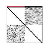
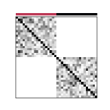
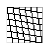
Figure 1: Left: Visualization of a matrix describedin Section 4.2 for which Algorithm 1 is not the best method for recovering the diagonal (intensity indicates magnitude of entries of $\mathbf{A}$). In particular, the diagonal of the matrix can be recovered using exactly 2 queries, while Algorithm 1 will require many queries to overcome the large noise in the off-diagonal blocks. Middle: Visualization of a matrix for which using the same colorings as the matrix on the left panel will not help. Right: Visualization of the hard sparsity pattern described in Section 4.3 with $k=10$. Here black pixels correspond to one and white pixels to zero. Note that while each row and column of the matrix has only $O(k)$ nonzeros, each pair of the $k^{2}$ columns has overlapping support.

In particular, for any integer $k\geq 1$, define the $k^{2}\times k^{2}$ matrix $\mathbf{A}$ by

$$[\mathbf{A}]_{pk+i,qk+j}=\begin{cases}1&i=q\text{ or }j=p\\ 0&\text{otherwise}\end{cases},\qquad p,q,i,j\in[k].$$

This sparsity pattern is represented in the left panel of Figure 1. Any given row or column of this matrix has exactly $s=2k-1$ nonzeros. However, the support of every column overlaps. Indeed, for columns $x=pk+i$ and $y=qk+j$ (with $i,j\in[k]$),

$$[\mathbf{A}]_{ik+q,x}=[\mathbf{A}]_{jk+p,y}=1,\quad[\mathbf{A}]_{jk+p,x}=[\mathbf{A}]_{ik+q,y}=1.$$

Therefore, exact coloring based approaches require $d=k^{2}=O(s^{2})$ colors; i.e. they do no better than the trivial upper bound of $d$ queries. In contrast, Algorithm 1 would require only $s$ queries.

5 Numerical Experiments

In this section we provide several numerical experiments which illustrate the performance of Algorithm 1. These problems are modeled after similar problems from the literature. Code to reproduce the figures can be found at https://github.com/tchen-research/fixed_sparsity_matrix_recovery.

5.1 Model problem

We consider the matrix $\mathbf{A}=\mathbf{M}^{-1}$, where $\mathbf{M}=\operatorname{tridiag}(-1,4,-1)$. This class of matrices exhibits exponential decay away from the diagonal and was used in experiments in past work [BS15, FSS21].

We take $\mathbf{A}$ to be $1000\times 1000$ and, for varying values of $b\geq 0$, we set $\mathbf{S}$ to be a symmetric banded matrix of maximum total bandwidth $2b+1$; i.e. $[\mathbf{S}]_{i,j}=\mathds{1}(|i-j|\leq b)$. We then compute the approximation error $\|\mathbf{A}-\widetilde{\mathbf{A}}\|_{\mathsf{F}}$ and recovery error $\|\mathbf{S}\circ\mathbf{A}-\widetilde{\mathbf{A}}\|_{\mathsf{F}}$ for the output of Algorithm 1 run using a varying number of matvec queries $m$.

The results are illustrated in Figure 2. Here the convergence of Algorithm 1 is matched well by the upper bound in Theorem 1 for the expected squared error (note that the plot shows the error, not the expected squared error).

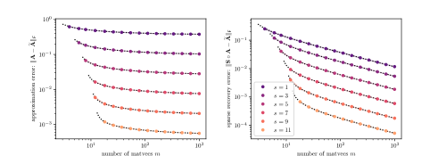
Figure 2: Approximation of model problem matrix $\mathbf{A}=\operatorname{tridiag}(-1,4,-1)^{-1}$ by a matrix of total bandwidth $s$ for varying values of $s$. The solid circles indicate the root mean squared error of Algorithm 1 over 20 independent runs of the algorithm, and the shaded region indicates the 10%-90% range. The dotted lines are the $\sqrt{s/(m-s-1)}\|\mathbf{A}-\mathbf{S}\circ\widetilde{\mathbf{A}}\|_{\mathsf{F}}$ (left) and $\sqrt{1+s/(m-s-1)}\|\mathbf{A}-\mathbf{S}\circ\widetilde{\mathbf{A}}\|_{\mathsf{F}}$ (right).

5.2 Trefethen Primes

We let $\mathbf{A}=\mathbf{M}^{-1}$, where $\mathbf{M}$ be the $1000\times 1000$ matrix whose entries are zero everywhere except for the primes $2,3,5,7,\ldots,7919$ along the main diagonal and the number 1 in all the positions $[\mathbf{B}]_{i,j}$ with $|i–j|\in\{1,2,4,8,\ldots,512\}$. An example (somewhat different from our example) involving this matrix was used in [PN23].

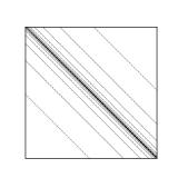
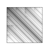
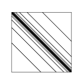
Figure 3: Left: Log-scale of the nonzero entries of $\mathbf{M}$, which range in magnitude from 1 to 7919. Middle: Log-scale of the nonzero entries of $\mathbf{A}$. Right: Sample sparsity pattern $\mathbf{S}$ corresponding to $b=5$.

For $b>0$, we defined a sparsity pattern $\mathbf{S}$ to be such that, for each $t\in\{1,2,4,8,\ldots,512\}$, $[\mathbf{S}]_{i,j}=1$ whenever $|i-j\pm t|\leq b$ and zero otherwise. In other words, the sparsity pattern consists of bandwidth $2b+1$ bands centered nonzero entries of $\mathbf{M}=\mathbf{A}^{-1}$. This is illustrated in Figure 3.

The results are shown in Figure 4. Here, the convergence of Algorithm 1 is somewhat better than the upper bound Theorem 1. This is because many rows of the sparsity pattern have far fewer than $s$ entries. From the proof of Theorem 1, it is clear how to obtain an exact characterization of the expected squared error.

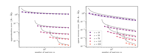
Figure 4: Approximation of “Trefethen primes” inverse matrix by a multi-banded matrix for varying values of $s$. The solid circles indicate the root mean squared error of Algorithm 1 over 100 independent runs of the algorithm, and the shaded region indicates the 10%-90% range. The dotted lines are the $\sqrt{s/(m-s-1)}\|\mathbf{A}-\mathbf{S}\circ\widetilde{\mathbf{A}}\|_{\mathsf{F}}$ (left) and $\sqrt{1+s/(m-s-1)}\|\mathbf{A}-\mathbf{S}\circ\widetilde{\mathbf{A}}\|_{\mathsf{F}}$ (right).

6 Outlook

This work raises a number of interesting practical and theoretical questions. We now comment on three.

It is clear that there is potential for combining coloring methods with algorithms such as Algorithm 1 in order to avoid paying for large off-sparsity entries in parts of a matrix while simultaneously maintaining the robustness to noise enjoyed by Algorithm 1. One approach to combining these two paradigms is to use adaptive queries to identify portions of the matrix with large-mass, and then find a coloring based on this information. We believe further study in this direction may yield algorithms which work better in many practical situations. Of course, our lower bound Theorem 2 shows that only constant factors can be improved for some families of problem instances.

The present paper focuses only on the Frobenius norm. It would be valuable to understand the analogous problem in other norms such as the matrix 2-norm. For other norms, $\mathbf{S}\circ\mathbf{A}$ is not necessarily the best approximation to $\mathbf{A}$ with sparsity $\mathbf{S}$. For instance, if $\mathbf{A}=[1,1;1,1]$ and $\mathbf{S}=[1,0;0,0]$, then

$$\operatornamewithlimits{argmin}_{\mathbf{X}=\mathbf{S}\circ\mathbf{X}}\|\mathbf{A}-\mathbf{X}\|_{2}=\begin{bmatrix}2&0\\ 0&0\end{bmatrix}\neq\begin{bmatrix}1&0\\ 0&0\end{bmatrix}=\mathbf{S}\circ\mathbf{A}.$$

Loosely speaking, minimizing the operator-norm approximation error requires the rows of the error matrix to be small and unaligned, whereas the Frobenius norm problem only requires them to be small.

Finally, it is of broad interest to understand algorithms and lower bounds for richer structures of matrices, such as the sum of sparse and low-rank matrices and matrices with hierarchical low-rank structure. This paper is a starting point for investigating these problems, and we hope that future work will explore them in greater depth.

Appendix A Lower Bound Lemmas

In this section, we provide the proofs of the key lemmas used the prove the lower bounds stated in Section 3. These lemmas are all standard in the literature, but we include the proofs for the benefit of the reader, as they are, for the most part, self-contained and interesting.

A.1 Adaptive queries to Wishart matrices

In this section we provide a proof of Proposition 3, which is essentially [BHSW20, Lemma 3.4]. This is mostly included for completeness. First, however, we consider what happens after a single non-adaptive query.

Lemma 3.

Suppose $\mathbf{G}\sim\operatorname{Gaussian}(d)$. Let $\mathbf{x}$ be a unit-length query chosen independently of $\mathbf{G}$, and define $\mathbf{y}=\mathbf{G}^{\mathsf{T}}\mathbf{G}\mathbf{x}$. Then, there is is an $n\times n$ orthonormal matrix $\hat{\mathbf{X}}=[\mathbf{x}~{}\mathbf{X}]$, constructed solely as a function of $\mathbf{x}$, and a matrix $\mathbf{H}\sim\operatorname{Gaussian}(n-1)$ independent of $\mathbf{x}$ and $\mathbf{y}$ such that such that

$$\hat{\mathbf{X}}^{\mathsf{T}}\mathbf{G}^{\mathsf{T}}\mathbf{G}\hat{\mathbf{X}}=\begin{bmatrix}\mathbf{x}^{\mathsf{T}}\mathbf{y}&\mathbf{y}^{\mathsf{T}}\mathbf{X}\\ \mathbf{X}^{\mathsf{T}}\mathbf{y}&(\mathbf{x}^{\mathsf{T}}\mathbf{y})^{-2}\mathbf{X}^{\mathsf{T}}\mathbf{y}\mathbf{y}^{\mathsf{T}}\mathbf{X}\end{bmatrix}+\begin{bmatrix}0&\mathbf{0}_{1,d-1}\\ \mathbf{0}_{d-1,1}&\mathbf{H}^{\mathsf{T}}\mathbf{H}\end{bmatrix}.$$

Proof.

Solely based on $\mathbf{x}$, extend to an orthonormal matrix:

$$\hat{\mathbf{X}}=\begin{bmatrix}\mathbf{x}&\mathbf{X}\end{bmatrix}.$$

For instance, append the identity to $\mathbf{x}$, delete the first column which is dependent on the previous columns, then orthonormalize sequentially using Gram–Schmidt.

Since $\mathbf{y}=\mathbf{G}^{\mathsf{T}}\mathbf{G}\mathbf{x}$,

$$\hat{\mathbf{X}}^{\mathsf{T}}\mathbf{G}^{\mathsf{T}}\mathbf{G}\hat{\mathbf{X}}=\begin{bmatrix}\mathbf{x}^{\mathsf{T}}\mathbf{y}&\mathbf{y}^{\mathsf{T}}\mathbf{X}\\ \mathbf{X}^{\mathsf{T}}\mathbf{y}&\mathbf{X}^{\mathsf{T}}\mathbf{G}^{\mathsf{T}}\mathbf{G}\mathbf{X}\end{bmatrix}.$$

The first row and column of this matrix depend only on $\mathbf{x}$ and $\mathbf{y}$. We will now show $\mathbf{X}^{\mathsf{T}}\mathbf{G}^{\mathsf{T}}\mathbf{G}\mathbf{X}$ consists of a matrix depending on $\mathbf{x}$ and $\mathbf{y}$ and Gaussian matrix independent of $\mathbf{x}$ and $\mathbf{y}$.

Define $\mathbf{r}=\|\mathbf{G}\mathbf{x}\|^{-1}\mathbf{G}\mathbf{x}$, and note that $\|\mathbf{r}\|=1$. Solely based on $\mathbf{r}$, extend to an orthonormal matrix:

$$\hat{\mathbf{R}}=\begin{bmatrix}\mathbf{r}&\mathbf{R}\end{bmatrix}.$$

Since $\hat{\mathbf{R}}$ is orthonormal, $\mathbf{r}\mathbf{r}^{\mathsf{T}}+\mathbf{R}\mathbf{R}^{\mathsf{T}}=\mathbf{I}$, and

$$\mathbf{X}^{\mathsf{T}}\mathbf{G}^{\mathsf{T}}\mathbf{G}\mathbf{X} =\mathbf{X}^{\mathsf{T}}\mathbf{G}^{\mathsf{T}}\mathbf{r}\mathbf{r}^{\mathsf{T}}\mathbf{G}\mathbf{X}+\mathbf{X}^{\mathsf{T}}\mathbf{G}^{\mathsf{T}}\mathbf{R}\mathbf{R}^{\mathsf{T}}\mathbf{G}\mathbf{X}$$

$$=\|\mathbf{G}\mathbf{x}\|^{-2}\mathbf{X}^{\mathsf{T}}\mathbf{G}^{\mathsf{T}}\mathbf{G}\mathbf{x}\mathbf{x}^{\mathsf{T}}\mathbf{G}^{\mathsf{T}}\mathbf{G}\mathbf{X}+\mathbf{X}^{\mathsf{T}}\mathbf{G}^{\mathsf{T}}\mathbf{R}\mathbf{R}^{\mathsf{T}}\mathbf{G}\mathbf{X}.$$

Thus, using that $\|\mathbf{G}\mathbf{x}\|^{2}=\mathbf{x}^{\mathsf{T}}\mathbf{G}^{\mathsf{T}}\mathbf{G}\mathbf{x}=\mathbf{x}^{\mathsf{T}}\mathbf{y}$,

$$\hat{\mathbf{X}}^{\mathsf{T}}\mathbf{G}^{\mathsf{T}}\mathbf{G}\hat{\mathbf{X}}=\begin{bmatrix}\mathbf{x}^{\mathsf{T}}\mathbf{y}&\mathbf{y}^{\mathsf{T}}\mathbf{X}\\ \mathbf{X}^{\mathsf{T}}\mathbf{y}&(\mathbf{x}^{\mathsf{T}}\mathbf{y})^{-2}\mathbf{X}^{\mathsf{T}}\mathbf{y}\mathbf{y}^{\mathsf{T}}\mathbf{X}\end{bmatrix}+\begin{bmatrix}0&\mathbf{0}_{1,n-1}\\ \mathbf{0}_{n-1,1}&\mathbf{X}^{\mathsf{T}}\mathbf{G}^{\mathsf{T}}\mathbf{R}\mathbf{R}^{\mathsf{T}}\mathbf{G}\mathbf{X}\end{bmatrix}.$$

It remains to show $\mathbf{R}^{\mathsf{T}}\mathbf{G}\mathbf{X}$ is a $(n-1)\times(n-1)$ Gaussian matrix independent of $\mathbf{x}$ and $\mathbf{y}$.

First, note that since ${\mathbf{X}}$ is chosen only based on $\mathbf{x}$ (which is independent of $\mathbf{G}$), $\mathbf{G}\hat{\mathbf{X}}$ consists of iid Gaussians. Thus, the columns of $\mathbf{G}{\mathbf{X}}$ are mutually independent of one another and $\mathbf{x}$, and hence $\mathbf{G}\mathbf{X}$ is mutually independent of $\mathbf{x}$ and $\mathbf{y}$. Finally, since $\mathbf{R}$ depends only on $\mathbf{r}=(\mathbf{x}^{\mathsf{T}}\mathbf{y})^{-1}\mathbf{G}\mathbf{x}$, $\mathbf{R}$ is independent of $\mathbf{G}\mathbf{X}$. Thus, $\mathbf{R}^{\mathsf{T}}\mathbf{G}\mathbf{X}$ has iid Gaussian entries independent of $\mathbf{x}$ and $\mathbf{y}$ (and hence any matrices constructed solely from $\mathbf{x}$ and $\mathbf{y}$). ∎

We will now prove the general statement.

Proof of Proposition 3.

We proceed by induction. Suppose, at step $t$ the result of the lemma holds. Let $\mathbf{x}_{t+1}$ be a query chosen based solely on $\mathbf{x}_{1},\ldots,\mathbf{x}_{t}$ and $\mathbf{y}_{1},\ldots,\mathbf{y}_{t}$ and hence independent of $\mathbf{G}_{t}$.

Then,

$$\mathbf{G}^{\mathsf{T}}\mathbf{G}\mathbf{x}_{t+1}=\mathbf{V}_{t}\mathbf{\Delta}_{t}\mathbf{V}_{t}^{\mathsf{T}}\mathbf{x}_{t+1}+\mathbf{V}_{t}^{\mathsf{T}}\begin{bmatrix}\mathbf{0}_{t,t}&\mathbf{0}_{t,d-t}\\ \mathbf{0}_{d-t,t}&\mathbf{G}_{t}^{\mathsf{T}}\mathbf{G}_{t}\end{bmatrix}\mathbf{V}_{t}^{\mathsf{T}}\mathbf{x}_{t+1}.$$

Let $\mathbf{x}$ denote the bottom $d-t$ entries of $\mathbf{V}^{\mathsf{T}}\mathbf{x}_{t+1}$, normalized to have length 1. By Lemma 3 the query to $\mathbf{G}_{t}^{\mathsf{T}}\mathbf{G}_{t}$ results in a factorization

$$\hat{\mathbf{X}}^{\mathsf{T}}\mathbf{G}_{t}^{\mathsf{T}}\mathbf{G}_{t}\hat{\mathbf{X}}=\mathbf{\Delta}+\begin{bmatrix}0&\mathbf{0}_{1,d-t-1}\\ \mathbf{0}_{d-t-1,1}&\mathbf{H}^{\mathsf{T}}\mathbf{H}\end{bmatrix},$$

where $\mathbf{\Delta}$ and $\hat{\mathbf{X}}$ are constructed solely as functions of $\mathbf{x}$ and $\mathbf{G}_{t}^{\mathsf{T}}\mathbf{G}_{t}\mathbf{x}$ (and hence of $\mathbf{x}_{1},\ldots,\mathbf{x}_{t+1}$ and $\mathbf{y}_{1},\ldots,\mathbf{y}_{t+1}$), $\hat{\mathbf{X}}$ is orthonormal, and $\mathbf{H}\sim\operatorname{Gaussian}(d-t-1)$ is independent of $\mathbf{x}$ (and hence of $\mathbf{x}_{1},\ldots,\mathbf{x}_{t+1}$ and $\mathbf{y}_{1},\ldots,\mathbf{y}_{t+1}$).

Define $\mathbf{G}_{t+1}=\mathbf{H}$ and the matrices

$$\widetilde{\mathbf{X}}=\begin{bmatrix}1&\mathbf{0}_{1,t-1}\\ \mathbf{0}_{t-1,t}&\hat{\mathbf{X}}\end{bmatrix},\qquad\mathbf{V}_{t+1}=\mathbf{V}_{t}\widetilde{\mathbf{X}},\quad\mathbf{\Delta}_{t+1}=\widetilde{\mathbf{X}}^{\mathsf{T}}\mathbf{\Delta}_{t}\widetilde{\mathbf{X}}+\begin{bmatrix}\mathbf{0}_{t,t}&\mathbf{0}_{t,d-t}\\ \mathbf{0}_{d-t,t}&\mathbf{\Delta}\end{bmatrix}.$$

Clearly $\mathbf{V}_{t+1}$ is orthonormal and $\mathbf{V}_{t+1}$ and $\mathbf{\Delta}_{t+1}$ are constructed solely as functions of $\mathbf{x}_{1},\ldots,\mathbf{x}_{t+1}$ and $\mathbf{y}_{1},\ldots,\mathbf{y}_{t+1}$ We easily verify that

$$\mathbf{V}_{t+1}^{\mathsf{T}}\mathbf{G}^{\mathsf{T}}\mathbf{G}\mathbf{V}_{t+1}=\widetilde{\mathbf{X}}^{\mathsf{T}}\mathbf{\Delta}_{t}\widetilde{\mathbf{X}}+\begin{bmatrix}\mathbf{0}_{t,t}&\mathbf{0}_{t,d-t}\\ \mathbf{0}_{d-t,t}&\hat{\mathbf{X}}^{\mathsf{T}}\mathbf{G}_{t}^{\mathsf{T}}\mathbf{G}_{t}\hat{\mathbf{X}}\end{bmatrix}=\mathbf{\Delta}_{t+1}+\begin{bmatrix}\mathbf{0}_{t+1,t+1}&\mathbf{0}_{t+1,d-(t+1)}\\ \mathbf{0}_{d-(t+1),t+1}&\mathbf{G}_{t+1}^{\mathsf{T}}\mathbf{G}_{t+1}\end{bmatrix}$$

The result is proved as the base case $t=0$ is trivial. ∎

A.2 Anti-concentration for sums

In this section we will prove Propositions 4 and 1.

We begin recalling the Berry–Esseen Theorem for non-identically distributed summands.

Proposition 5 (Berry–Esseen; see e.g. [Ser80, §1.9]).

There exists a constant $C>0$ such that, if $X_{1},\ldots,X_{k}$ are independent random variables with $\operatorname{\mathbb{E}}[X_{i}]=0$, $\operatorname{\mathbb{E}}[X_{i}^{2}]=\sigma_{i}^{2}$, and $\operatorname{\mathbb{E}}[|X_{i}|^{3}]=\rho_{i}$, and if we define

$$Y=\frac{X_{1}+\cdots+X_{k}}{(\sigma_{1}^{2}+\cdots+\sigma_{k}^{2})^{1/2}},$$

then the CDF $F_{Y}$ of $Y$ is near to the CDF $\Phi$ of a standard Gaussian in that,

$$\forall z:|F_{Y}(z)-\Phi(z)|\leq C\frac{\rho_{1}+\cdots+\rho_{k}}{(\sigma_{1}^{2}+\cdots+\sigma_{k}^{2})^{3/2}}.$$

In addition, we note a simple anti-concentration bound for Gaussians.

Lemma 4.

Let $Z\sim\mathcal{N}(0,1)$. Then, for any $t\in\mathbb{R}$ and any $\alpha>0$,

$$\operatorname{\mathbb{P}}\Bigl{[}|Z-t|<\alpha\Bigr{]}<\sqrt{\frac{2}{\pi}}\,\alpha.$$

Proof.

Note that the density for $Z$ is $f_{Z}(x)=(1/\sqrt{2\pi})\exp(-x^{2}/2)$, and $f_{Z}(x)\leq 1/\sqrt{2\pi}$ for all $x$. Hence,

$$\operatorname{\mathbb{P}}\bigl{[}|Z-t|<\alpha\bigr{]}=\int_{t-\alpha}^{t+\alpha}f_{Z}(x)\mathrm{d}{x}\leq\frac{2\alpha}{\sqrt{2\pi}}=\sqrt{\frac{2}{\pi}}\alpha.\qed$$

Proof of Proposition 4.

Without loss of generality, we can assume $\operatorname{\mathbb{E}}[X_{i}]=0$ for all $i$ by absorbing the means into $t$. By assumption we have that

$$\hat{\sigma}=\sqrt{\sigma_{1}^{2}+\cdots+\sigma_{k}^{2}}\geq\sigma\sqrt{k},\qquad\rho_{1}+\cdots+\rho_{k}\leq k\rho.$$

Let $Y=X/\hat{\sigma}$ with cumulative distribution $F_{Y}$ and let $t^{\prime}=t/\hat{\sigma}$. Then, with $C$ denoting the constant from Proposition 5, we apply Proposition 5, Lemma 4, and the bounds above to obtain

$$\operatorname{\mathbb{P}}\bigl{[}|X-t|<\alpha\sigma\sqrt{k}\bigr{]} \leq\operatorname{\mathbb{P}}\bigl{[}|X-t|<\alpha\hat{\sigma}\bigr{]}$$

$$=\operatorname{\mathbb{P}}\bigl{[}|Y-t^{\prime}|<\alpha\bigr{]}$$

$$=F_{Y}(t^{\prime}+\alpha)-F_{Y}(t^{\prime}-\alpha)$$

$$\leq\Phi(t^{\prime}+\alpha)-\Phi(t^{\prime}-\alpha)+\frac{2Ck\rho}{k^{3/2}\sigma^{3}}$$

$$\leq\sqrt{\frac{2}{\pi}}\alpha+\frac{2C\rho}{\sigma^{3}\sqrt{k}}.$$

Since $(1-\sqrt{2/\pi})>0.2$, the result follows by the choice $k>100C^{2}\rho^{2}/(\alpha^{2}\sigma^{6})$, and relabeling $C$. ∎

Proof of Lemma 1.

Let $\mathbf{g}_{\ell}$ denote the $\ell$-th row of $\mathbf{G}$ and define $x_{\ell}=\mathbf{u}^{\mathsf{T}}\mathbf{g}_{\ell}$ and $y_{\ell}=\mathbf{v}^{\mathsf{T}}\mathbf{g}_{\ell}$. In order to apply Proposition 4 to the sum

$$\mathbf{x}^{\mathsf{T}}\mathbf{y}=\sum_{\ell=1}^{k}x_{\ell}y_{\ell},$$

which has independent terms since the $\mathbf{g}_{\ell}$ are independent, we must obtain upper-and lower-bounds on the variance and an upper bound on the third centered absolute moment of each term.

We will first bound the variance. By direct computation (see Fact 1 for a derivation),

$$\operatorname{\mathbb{V}}\bigl{[}x_{\ell}y_{\ell}\bigr{]}=\operatorname{\mathbb{V}}\bigl{[}\mathbf{g}_{\ell}^{\mathsf{T}}\mathbf{v}\mathbf{u}^{\mathsf{T}}\mathbf{g}_{\ell}\bigr{]}=\|\mathbf{v}\mathbf{u}^{\mathsf{T}}+\mathbf{u}\mathbf{v}^{\mathsf{T}}\|_{\mathsf{F}}^{2}/2\geq\|\mathbf{u}\|_{2}^{2}\|\mathbf{v}\|_{2}^{2}.$$

Here we have used that

$$\|\mathbf{v}\mathbf{u}^{\mathsf{T}}+\mathbf{u}\mathbf{v}^{\mathsf{T}}\|_{\mathsf{F}}^{2}=2\|\mathbf{v}\mathbf{u}^{\mathsf{T}}\|_{\mathsf{F}}^{2}+2(\mathbf{v}^{\mathsf{T}}\mathbf{u})^{2}\geq 2\|\mathbf{v}\|_{2}^{2}\|\mathbf{u}\|_{2}^{2}.$$

We now argue the third absolute moments are bounded. Note that $x_{\ell}$ and $y_{\ell}$ are both normally distributed with mean zero and variance at most $1$ (since $\|\mathbf{u}\|_{2}\leq 1$ and $\|\mathbf{v}\|_{2}\leq 1$). Then $x_{\ell}y_{\ell}$ is sub-exponential with constant width parameter [Ver18, Lemma 2.7.7], and hence $\operatorname{\mathbb{E}}[|x_{\ell}y_{\ell}-\operatorname{\mathbb{E}}[x_{\ell}y_{\ell}]|^{3}]\leq\rho$ for some $\rho$.

Hence, applying Proposition 4, for any $\alpha>0$, and provided $k>C\rho^{2}/(\alpha^{2}\|\mathbf{u}\|_{2}^{6}\|\mathbf{v}\|_{2}^{6})$, where $C$ is the constant from Proposition 4,

$$\operatorname{\mathbb{P}}\Bigl{[}\big{|}\mathbf{x}^{\mathsf{T}}\mathbf{y}-t\big{|}<\alpha\|\mathbf{u}\|_{2}\|\mathbf{v}\|_{2}\sqrt{k}\Bigr{]}<\alpha.$$

Relabeling $C$ gives the result. ∎

A.3 Other facts

Fact 1.

For a matrix $\mathbf{A}\in\mathbb{R}^{d\times d}$, if $\mathbf{g}\sim\operatorname{Gaussian}(d,1)$, then $\operatorname{\mathbb{V}}[\mathbf{g}^{\mathsf{T}}\mathbf{A}\mathbf{g}]=\|\mathbf{A}+\mathbf{A}^{\mathsf{T}}\|_{\mathsf{F}}^{2}/2$.

Proof.

Since $\mathbf{g}^{\mathsf{T}}\mathbf{A}\mathbf{g}=\mathbf{g}^{\mathsf{T}}(\mathbf{A}^{\mathsf{T}}+\mathbf{A})\mathbf{g}/2$, without loss of generality we can assume $\mathbf{A}$ is symmetric. Let $\mathbf{A}=\mathbf{U}\mathbf{\Lambda}\mathbf{U}^{\mathsf{T}}$ be the eigendecomposition of $\mathbf{A}$, then $\mathbf{h}=\mathbf{U}^{\mathsf{T}}\mathbf{g}\sim\operatorname{Gaussian}(d,1)$ and $\mathbf{h}^{\mathsf{T}}\mathbf{\Lambda}\mathbf{h}$ is a linear-combination of independent Chi-squared random variables with one degree of freedom (and variance 2). The result follows since $\|\mathbf{A}\|_{\mathsf{F}}^{2}=\|\mathbf{\Lambda}\|_{\mathsf{F}}^{2}$. ∎

Fact 2.

For $d\geq 1$, suppose $\mathbf{G}\sim\operatorname{Gaussian}(d)$. Then $\operatorname{\mathbb{E}}[\|\mathbf{G}^{\mathsf{T}}\mathbf{G}\|_{\mathsf{F}}^{2}]\leq 3d^{3}$.

Proof.

Write $\mathbf{A}=\mathbf{G}^{\mathsf{T}}\mathbf{G}$. The diagonal entries of $\mathbf{A}$ are distributed as Chi-squared random variables with $d$ degrees of freedom. These entries have mean $d$ and variance $2d$. Likewise, the off-diagonal entries of $\mathbf{A}$ are distributed as the inner product of two independent standard normal Gaussian vectors of length $d$. These entries therefore have mean zero and variance $d$. Therefore, for $i\neq j$,

$$\operatorname{\mathbb{E}}\bigl{[}[\mathbf{A}]_{i,i}^{2}\bigr{]}=\operatorname{\mathbb{V}}\bigl{[}[\mathbf{A}]_{i,i}\bigr{]}+\operatorname{\mathbb{E}}\bigl{[}[\mathbf{A}]_{i,i}\bigr{]}^{2}=2d+d^{2},\qquad\operatorname{\mathbb{E}}\bigl{[}[\mathbf{A}]_{i,j}^{2}\bigr{]}=\operatorname{\mathbb{V}}\bigl{[}[\mathbf{A}]_{i,j}\bigr{]}=d.$$

By the linearity of expectation,

$$\operatorname{\mathbb{E}}\bigl{[}\|\mathbf{A}\|_{\mathsf{F}}^{2}\bigr{]}=\sum_{i=1}^{d}\sum_{j=1}^{d}\operatorname{\mathbb{E}}\bigl{[}[\mathbf{A}]_{i,j}^{2}\bigr{]}=d\cdot(2d+d^{2})+(d^{2}-d)\cdot d\leq 3d^{3}.\qed$$

Appendix B High probability algorithm

The bound Theorem 1 for Algorithm 1 has an unfavorable dependence $O(1/\delta)$ on the failure probability $\delta$. We will now use a high-dimensional version of the “median trick” to improve the dependence on the failure probability to logarithmic.

Algorithm 2 Fixed-sparse-matrix recovery (boosted)

1:procedure boosted-fixed-sparse-matrix recovery($\mathbf{A},\mathbf{S},m,r$)

2:     Run Algorithm 1 independently $r$ times to get $\widetilde{\mathbf{A}}_{1},\ldots,\widetilde{\mathbf{A}}_{r}$

3:     $\forall i,j$: define $d_{i,j}=\|\widetilde{\mathbf{A}}_{i}-\widetilde{\mathbf{A}}_{j}\|_{\mathsf{F}}$

4:     $\forall i$: define $B_{i}$ as the $\lceil r/2\rceil$-th smallest $d_{i,j}$ $\triangleright$ $\big{|}\{j\in[r]:d_{i,j}\leq B_{i}\}\big{|}=\lceil r/2\rceil$

5:     Compute $i^{*}=\operatornamewithlimits{argmin}_{i}B_{i}$ $\triangleright$ $\forall i:B_{i^{*}}\leq B_{i}$

6:return $\widetilde{\mathbf{A}}_{i^{*}}$

Theorem 3.

Consider any $\mathbf{A}\in\mathbb{R}^{n\times d}$ and any $\mathbf{S}\in\{0,1\}^{n\times d}$ with at most $s$ nonzero entries per row. For any $\varepsilon>0$ and $\delta\in(0,1)$, if $m\geq s+2$ and additionally

$$m\geq s\left(\frac{90}{\varepsilon}+1\right)+1,\quad r\geq 10\log\left(\frac{1}{\delta}\right),$$

then, using $m\cdot r$ matrix-vector queries, Algorithm 2 returns a matrix $\widetilde{\mathbf{A}}$ satisfying:

$$\operatorname{\mathbb{P}}\bigl{[}\|\mathbf{A}-\widetilde{\mathbf{A}}\|_{\mathsf{F}}<(1+\varepsilon)\|\mathbf{A}-\mathbf{S}\circ\mathbf{A}\|_{\mathsf{F}}\bigr{]}\geq 1-\delta.$$

Proof.

Let $\tilde{\varepsilon}=\frac{2}{9}\varepsilon$. Define the set

$$P=\big{\{}i\in[r]:\|\mathbf{S}\circ\mathbf{A}-\widetilde{\mathbf{A}}_{i}\|_{\mathsf{F}}^{2}\leq\tilde{\varepsilon}\|\mathbf{A}-\mathbf{S}\circ\mathbf{A}\|_{\mathsf{F}}^{2}\big{\}}.$$

In Equation 6 of the proof of Corollary 1, we show that

$$\operatorname{\mathbb{P}}\bigl{[}\|\mathbf{S}\circ\mathbf{A}-\widetilde{\mathbf{A}}_{i}\|_{\mathsf{F}}^{2}\geq\varepsilon\|\mathbf{A}-\mathbf{S}\circ\mathbf{A}\ |_{\mathsf{F}}^{2}\bigr{]}\leq s/\big{(}(m-s-1)\tilde{\varepsilon}\big{)}.$$

Hence, if $m\geq s((20/\tilde{\varepsilon})+1)+1$, then $\operatorname{\mathbb{P}}[i\in P]\geq\frac{19}{20}$. Define the event

$$E=\{|P|>\lfloor r/2\rfloor\}.$$

A standard result [AV79, Prop 2.4 (a)] asserts that with $q=19/20$,

$$\sum_{k=0}^{\lfloor r/2\rfloor}\binom{r}{k}q^{k}(1-q)^{r-k}\leq\exp\left(-\frac{rq}{2}\left(1-\frac{1}{2q}\right)^{2}\right)=\exp\left(-\frac{81r}{760}\right).$$

In addition, $\delta\geq\exp(-r/10)$ by definition of $r$. Therefore, $\operatorname{\mathbb{P}}[E]\geq 1-\delta$.

We will condition on $E$ for the remainder of the proof. By the triangle inequality, for any indices $i,j\in P$,

$$d_{i,j}=\|\widetilde{\mathbf{A}}_{i}-\widetilde{\mathbf{A}}_{j}\|_{\mathsf{F}}\leq\|\widetilde{\mathbf{A}}_{i}-\mathbf{S}\circ\mathbf{A}\|_{\mathsf{F}}+\|\mathbf{S}\circ\mathbf{A}-\widetilde{\mathbf{A}}_{j}\|_{\mathsf{F}}\leq 2\sqrt{\varepsilon}\|\mathbf{A}-\mathbf{S}\circ\mathbf{A}\|_{\mathsf{F}}.$$

Since $|P|>\lfloor r/2\rfloor$, then for each $i\in P$, there are at least $\lfloor r/2\rfloor$ indices $j$ satisfying $d_{i,j}\leq 2\sqrt{\varepsilon}\|\mathbf{A}-\mathbf{S}\circ\mathbf{A}\|_{\mathsf{F}}$. Thus by definition of $B_{i}$,

$$B_{i}\leq 2\sqrt{\tilde{\varepsilon}}\|\mathbf{A}-\mathbf{S}\circ\mathbf{A}\|_{\mathsf{F}}.$$

By definition of $B_{i^{*}}$, there are at least $\lceil r/2\rceil$ indices $j$ for which

$$\|\widetilde{\mathbf{A}}_{i^{*}}-\widetilde{\mathbf{A}}_{j}\|_{\mathsf{F}}\leq 2\sqrt{\tilde{\varepsilon}}\|\mathbf{A}-\mathbf{S}\circ\mathbf{A}\|_{\mathsf{F}}$$

Simultaneously, $|P|>\lfloor r/2\rfloor$. Since $|P|+\lceil r/2\rceil>\lfloor r/2\rfloor+\lceil r/2\rceil=r$, the pigeonhole principle ensures there is at least one $j^{*}$ for which $j^{*}\in P$ and

$$\|\widetilde{\mathbf{A}}_{i^{*}}-\widetilde{\mathbf{A}}_{j^{*}}\|_{\mathsf{F}}\leq 2\sqrt{\tilde{\varepsilon}}\|\mathbf{A}-\mathbf{S}\circ\mathbf{A}\|_{\mathsf{F}}.$$

Applying the triangle inequality, we find that

$$\|\mathbf{S}\circ\mathbf{A}-\widetilde{\mathbf{A}}_{i^{*}}\|_{\mathsf{F}}\leq\|\mathbf{S}\circ\mathbf{A}-\widetilde{\mathbf{A}}_{j^{*}}\|_{\mathsf{F}}+\|\widetilde{\mathbf{A}}_{i^{*}}-\widetilde{\mathbf{A}}_{j^{*}}\|_{\mathsf{F}}\leq 3\sqrt{\tilde{\varepsilon}}\|\mathbf{A}-\mathbf{S}\circ\mathbf{A}\|_{\mathsf{F}}.$$

which implies $\|\mathbf{S}\circ\mathbf{A}-\widetilde{\mathbf{A}}_{i^{*}}\|_{\mathsf{F}}^{2}\leq 9\tilde{\varepsilon}\|\mathbf{A}-\mathbf{S}\circ\mathbf{A}\|_{\mathsf{F}}^{2}.$ Adding $\|\mathbf{A}-\mathbf{S}\circ\mathbf{A}\|_{\mathsf{F}}^{2}$ to both sides (see Equation 1) and taking square roots,

$$\|\mathbf{A}-\widetilde{\mathbf{A}}_{i^{*}}\|_{\mathsf{F}}\leq\sqrt{1+9\tilde{\varepsilon}}\|\mathbf{A}-\mathbf{S}\circ\mathbf{A}\|_{\mathsf{F}}=\sqrt{1+2\varepsilon}\|\mathbf{A}-\mathbf{S}\circ\mathbf{A}\|_{\mathsf{F}}\leq(1+\varepsilon)\|\mathbf{A}-\mathbf{S}\circ\mathbf{A}\|_{\mathsf{F}}.\qed$$

References

- [AV79] D. Angluin and L.G. Valiant “Fast Probabilistic Algorithms for Hamiltonian Circuits and Matchings” In Journal of Computer and System Sciences 18.2 Elsevier BV, 1979, pp. 155–193 DOI: 10.1016/0022-0000(79)90045-x
- [BBR13] Michele Benzi, Paola Boito and Nader Razouk “Decay Properties of Spectral Projectors with Applications to Electronic Structure” In SIAM Review 55.1 Society for Industrial & Applied Mathematics (SIAM), 2013, pp. 3–64 DOI: 10.1137/100814019
- [BCW22] Ainesh Bakshi, Kenneth L. Clarkson and David P. Woodruff “Low-Rank Approximation with Matrix-Vector Products” In Proceedings of the 54th Annual ACM SIGACT Symposium on Theory of Computing, STOC 2022 Rome, Italy: Association for Computing Machinery, 2022, pp. 1130–1143 DOI: 10.1145/3519935.3519988
- [BET22] Nicolas Boullé, Christopher J. Earls and Alex Townsend “Data-driven discovery of Green’s functions with human-understandable deep learning” In Sci. Rep. 12.1, 2022, pp. 4824
- [BHOT24] Nicolas Boullé, Diana Halikias, Samuel E. Otto and Alex Townsend “Operator learning without the adjoint”, 2024 arXiv:2401.17739 [math.NA]
- [BHSW20] Mark Braverman, Elad Hazan, Max Simchowitz and Blake Woodworth “The Gradient Complexity of Linear Regression” In Proceedings of Thirty Third Conference on Learning Theory 125, Proceedings of Machine Learning Research PMLR, 2020, pp. 627–647 URL: https://proceedings.mlr.press/v125/braverman20a.html
- [BHT23] Nicolas Boullé, Diana Halikias and Alex Townsend “Elliptic PDE learning is provably data-efficient” In Proceedings of the National Academy of Sciences 120.39, 2023, pp. e2303904120
- [BKS07] C. Bekas, E. Kokiopoulou and Y. Saad “An estimator for the diagonal of a matrix” In Applied Numerical Mathematics 57.11–12 Elsevier BV, 2007, pp. 1214–1229 DOI: 10.1016/j.apnum.2007.01.003
- [BN22] Robert A. Baston and Yuji Nakatsukasa “Stochastic diagonal estimation: probabilistic bounds and an improved algorithm”, 2022 arXiv:2201.10684 [cs.DS]
- [BN23] Ainesh Bakshi and Shyam Narayanan “Krylov Methods are (nearly) Optimal for Low-Rank Approximation” In 2023 IEEE 64th Annual Symposium on Foundations of Computer Science (FOCS) IEEE, 2023 DOI: 10.1109/focs57990.2023.00128
- [BR08] Michele Benzi and Nader Razouk “Decay bounds and algorithms for approximating functions of sparse matrices” In Electron. Trans. Numer. Anal. 28, 2007-2008, pp. 16–39
- [BS15] Michele Benzi and Valeria Simoncini “Decay Bounds for Functions of Hermitian Matrices with Banded or Kronecker Structure” In SIAM Journal on Matrix Analysis and Applications 36.3 Society for Industrial & Applied Mathematics (SIAM), 2015, pp. 1263–1282 DOI: 10.1137/151006159
- [BT99] Michele Benzi and Miroslav Tûma “A comparative study of sparse approximate inverse preconditioners” In Applied Numerical Mathematics 30.2–3 Elsevier BV, 1999, pp. 305–340 DOI: 10.1016/s0168-9274(98)00118-4
- [CC86] Thomas F. Coleman and Jin-Yi Cai “The Cyclic Coloring Problem and Estimation of Sparse Hessian Matrices” In SIAM Journal on Algebraic Discrete Methods 7.2 Society for Industrial & Applied Mathematics (SIAM), 1986, pp. 221–235 DOI: 10.1137/0607026
- [Che+23] Sinho Chewi, Jaume De Dios Pont, Jerry Li, Chen Lu and Shyam Narayanan “Query lower bounds for log-concave sampling” In 2023 IEEE 64th Annual Symposium on Foundations of Computer Science (FOCS) IEEE, 2023 DOI: 10.1109/focs57990.2023.00131
- [CM83] Thomas F. Coleman and Jorge J. Moré “Estimation of Sparse Jacobian Matrices and Graph Coloring Blems” In SIAM Journal on Numerical Analysis 20.1 Society for Industrial & Applied Mathematics (SIAM), 1983, pp. 187–209 DOI: 10.1137/0720013
- [CPR74] A.. Curtis, M… Powell and J.. Reid “On the Estimation of Sparse Jacobian Matrices” In IMA Journal of Applied Mathematics 13.1 Oxford University Press (OUP), 1974, pp. 117–119 DOI: 10.1093/imamat/13.1.117
- [CW09] Kenneth L Clarkson and David P Woodruff “Numerical linear algebra in the streaming model” In Proceedings of the Forty-First Annual ACM Symposium on Theory of Computing, 2009, pp. 205–214
- [DM23] Prathamesh Dharangutte and Christopher Musco “A Tight Analysis of Hutchinson’s Diagonal Estimator” In Symposium on Simplicity in Algorithms (SOSA) Society for IndustrialApplied Mathematics, 2023, pp. 353–364 DOI: 10.1137/1.9781611977585.ch32
- [DMS84] Stephen Demko, William F. Moss and Philip W. Smith “Decay rates for inverses of band matrices” In Mathematics of Computation 43.168 American Mathematical Society (AMS), 1984, pp. 491–499 DOI: 10.1090/s0025-5718-1984-0758197-9
- [DSBN15] Gautam Dasarathy, Parikshit Shah, Badri Narayan Bhaskar and Robert D. Nowak “Sketching Sparse Matrices, Covariances, and Graphs via Tensor Products” In IEEE Transactions on Information Theory 61.3 Institute of ElectricalElectronics Engineers (IEEE), 2015, pp. 1373–1388 DOI: 10.1109/tit.2015.2391251
- [EK12] Yonina C. Eldar and Gitta Kutyniok “Compressed sensing: theory and applications” Cambridge; New York: Cambridge University Press, 2012
- [ET23] Ethan N. Epperly and Joel A. Tropp “Efficient error and variance estimation for randomized matrix computations”, 2023 arXiv:2207.06342 [math.NA]
- [FR13] Simon Foucart and Holger Rauhut “A Mathematical Introduction to Compressive Sensing” In Applied and Numerical Harmonic Analysis Springer New York, 2013 DOI: 10.1007/978-0-8176-4948-7
- [FSS21] Andreas Frommer, Claudia Schimmel and Marcel Schweitzer “Analysis of Probing Techniques for Sparse Approximation and Trace Estimation of Decaying Matrix Functions” In SIAM Journal on Matrix Analysis and Applications 42.3 Society for Industrial & Applied Mathematics (SIAM), 2021, pp. 1290–1318 DOI: 10.1137/20m1364461
- [Gir87] Didier Girard “Un algorithme rapide pour le calcul de la trace de l’inverse d’une grande matrice”, 1987
- [Gre97] Anne Greenbaum “Iterative Methods for Solving Linear Systems” Philadelphia, PA, USA: Society for IndustrialApplied Mathematics, 1997
- [GS92] E. Gallopoulos and Y. Saad “Efficient Solution of Parabolic Equations by Krylov Approximation Methods” In SIAM Journal on Scientific and Statistical Computing 13.5 Society for Industrial & Applied Mathematics (SIAM), 1992, pp. 1236–1264 DOI: 10.1137/0913071
- [Hig08] Nicholas J. Higham “Functions of Matrices” Society for IndustrialApplied Mathematics, 2008 DOI: 10.1137/1.9780898717778
- [HIS23] Eric Hallman, Ilse C.. Ipsen and Arvind K. Saibaba “Monte Carlo Methods for Estimating the Diagonal of a Real Symmetric Matrix” In SIAM Journal on Matrix Analysis and Applications 44.1 Society for Industrial & Applied Mathematics (SIAM), 2023, pp. 240–269 DOI: 10.1137/22m1476277
- [HMT11] N. Halko, P.. Martinsson and J.. Tropp “Finding structure with randomness: probabilistic algorithms for constructing approximate matrix decompositions” In SIAM Rev. 53.2, 2011, pp. 217–288 DOI: 10.1137/090771806
- [HT23] Diana Halikias and Alex Townsend “Structured matrix recovery from matrix‐vector products” In Numerical Linear Algebra with Applications 31.1 Wiley, 2023 DOI: 10.1002/nla.2531
- [Hut89] M.F. Hutchinson “A Stochastic Estimator of the Trace of the Influence Matrix for Laplacian Smoothing Splines” In Communications in Statistics - Simulation and Computation 18.3 Informa UK Limited, 1989, pp. 1059–1076 DOI: 10.1080/03610918908812806
- [JPWZ21] Shuli Jiang, Hai Pham, David Woodruff and Richard Zhang “Optimal Sketching for Trace Estimation” In Advances in Neural Information Processing Systems 34 Curran Associates, Inc., 2021, pp. 23741–23753 URL: https://proceedings.neurips.cc/paper_files/paper/2021/file/c77bfda61a0204d445185053e6a9a8fe-Paper.pdf
- [Kar+21] George Em Karniadakis, Ioannis G Kevrekidis, Lu Lu, Paris Perdikaris, Sifan Wang and Liu Yang “Physics-informed machine learning” In Nat. Rev. Phys. 3.6 Nature Publishing Group, 2021, pp. 422–440
- [KK11] Willi A. Kalender and Willi A. Kalender “Computed tomography: fundamentals, system technology, image quality, applications; [including 64-slice spiral CT]” Erlangen: Publicis Publ, 2011
- [LLY11] Lin Lin, Jianfeng Lu and Lexing Ying “Fast construction of hierarchical matrix representation from matrix–vector multiplication” In Journal of Computational Physics 230.10 Elsevier BV, 2011, pp. 4071–4087 DOI: 10.1016/j.jcp.2011.02.033
- [LM22] James Levitt and Per-Gunnar Martinsson “Linear-Complexity Black-Box Randomized Compression of Rank-Structured Matrices”, 2022 arXiv:2205.02990 [math.NA]
- [LM22a] James Levitt and Per-Gunnar Martinsson “Randomized Compression of Rank-Structured Matrices Accelerated with Graph Coloring”, 2022 arXiv:2205.03406 [math.NA]
- [Mar16] Per-Gunnar Martinsson “Compressing Rank-Structured Matrices via Randomized Sampling” In SIAM Journal on Scientific Computing 38.4 Society for Industrial & Applied Mathematics (SIAM), 2016, pp. A1959–A1986 DOI: 10.1137/15m1016679
- [MMMW21] Raphael A. Meyer, Cameron Musco, Christopher Musco and David P. Woodruff “Hutch++: Optimal Stochastic Trace Estimation” In Symposium on Simplicity in Algorithms (SOSA) Society for IndustrialApplied Mathematics, 2021, pp. 142–155 DOI: 10.1137/1.9781611976496.16
- [MT20] Per-Gunnar Martinsson and Joel A. Tropp “Randomized numerical linear algebra: Foundations and algorithms” In Acta Numerica 29 Cambridge University Press (CUP), 2020, pp. 403–572 DOI: 10.1017/s0962492920000021
- [Mui82] Robb J. Muirhead “Aspects of Multivariate Statistical Theory” In Wiley Series in Probability and Statistics Wiley, 1982 DOI: 10.1002/9780470316559
- [Mur+23] Riley Murray, James Demmel, Michael W. Mahoney, N. Erichson, Maksim Melnichenko, Osman Asif Malik, Laura Grigori, Piotr Luszczek, Michał Dereziński, Miles E. Lopes, Tianyu Liang, Hengrui Luo and Jack Dongarra “Randomized Numerical Linear Algebra : A Perspective on the Field With an Eye to Software”, 2023 arXiv:2302.11474 [math.NA]
- [NSW22] Deanna Needell, William Swartworth and David P. Woodruff “Testing Positive Semidefiniteness Using Linear Measurements” In 2022 IEEE 63rd Annual Symposium on Foundations of Computer Science (FOCS) IEEE, 2022 DOI: 10.1109/focs54457.2022.00016
- [Pea94] Barak A. Pearlmutter “Fast Exact Multiplication by the Hessian” In Neural Computation 6.1 MIT Press - Journals, 1994, pp. 147–160 DOI: 10.1162/neco.1994.6.1.147
- [PN23] Taejun Park and Yuji Nakatsukasa “Approximating Sparse Matrices and their Functions using Matrix-vector products”, 2023 arXiv:2310.05625 [math.NA]
- [PW11] Eric Price and David P. Woodruff “(1 + eps)-Approximate Sparse Recovery” In 2011 IEEE 52nd Annual Symposium on Foundations of Computer Science IEEE, 2011 DOI: 10.1109/focs.2011.92
- [SER18] Max Simchowitz, Ahmed El Alaoui and Benjamin Recht “Tight query complexity lower bounds for PCA via finite sample deformed wigner law” In Proceedings of the 50th Annual ACM SIGACT Symposium on Theory of Computing, STOC ’18 ACM, 2018 DOI: 10.1145/3188745.3188796
- [Ser80] Robert J. Serfling “Approximation Theorems of Mathematical Statistics” In Wiley Series in Probability and Statistics Wiley, 1980 DOI: 10.1002/9780470316481
- [Ski89] John Skilling “The Eigenvalues of Mega-dimensional Matrices” In Maximum Entropy and Bayesian Methods Springer Netherlands, 1989, pp. 455–466 DOI: 10.1007/978-94-015-7860-8˙48
- [SKO21] Florian Schäfer, Matthias Katzfuss and Houman Owhadi “Sparse Cholesky Factorization by Kullback–Leibler Minimization” In SIAM Journal on Scientific Computing 43.3 Society for Industrial & Applied Mathematics (SIAM), 2021, pp. A2019–A2046 DOI: 10.1137/20m1336254
- [SLO13] Andreas Stathopoulos, Jesse Laeuchli and Kostas Orginos “Hierarchical Probing for Estimating the Trace of the Matrix Inverse on Toroidal Lattices” In SIAM Journal on Scientific Computing 35.5 Society for Industrial & Applied Mathematics (SIAM), 2013, pp. S299–S322 DOI: 10.1137/120881452
- [SO21] Florian Schäfer and Houman Owhadi “Sparse recovery of elliptic solvers from matrix-vector products”, 2021 arXiv:2110.05351 [math.NA]
- [SW23] William Swartworth and David P. Woodruff “Optimal Eigenvalue Approximation via Sketching” In Proceedings of the 55th Annual ACM Symposium on Theory of Computing, STOC ’23 ACM, 2023 DOI: 10.1145/3564246.3585102
- [SWYZ21] Xiaoming Sun, David P. Woodruff, Guang Yang and Jialin Zhang “Querying a Matrix through Matrix-Vector Products” In ACM Trans. Algorithms 17.4 Association for Computing Machinery, 2021
- [Tre02] Nick Trefethen “A Hundred-dollar, Hundred-digit Challenge” In SIAM News 35.1, 2002
- [TS11] Jok M. Tang and Yousef Saad “A probing method for computing the diagonal of a matrix inverse” In Numerical Linear Algebra with Applications 19.3 Wiley, 2011, pp. 485–501 DOI: 10.1002/nla.779
- [TW23] Joel A Tropp and Robert J Webber “Randomized algorithms for low-rank matrix approximation: Design, analysis, and applications” In arXiv preprint arXiv:2306.12418, 2023
- [Ver18] Roman Vershynin “High-Dimensional Probability” Cambridge University Press, 2018 DOI: 10.1017/9781108231596
- [WEV13] Thakshila Wimalajeewa, Yonina C. Eldar and Pramod K. Varshney “Recovery of Sparse Matrices via Matrix Sketching”, 2013 arXiv:1311.2448 [cs.NA]
- [WSB11] Andrew Waters, Aswin Sankaranarayanan and Richard Baraniuk “SpaRCS: Recovering low-rank and sparse matrices from compressive measurements” In Advances in Neural Information Processing Systems 24 Curran Associates, Inc., 2011 URL: https://proceedings.neurips.cc/paper_files/paper/2011/file/0ff8033cf9437c213ee13937b1c4c455-Paper.pdf
- [WWAF06] Alexander Weiße, Gerhard Wellein, Andreas Alvermann and Holger Fehske “The kernel polynomial method” In Reviews of Modern Physics 78.1 American Physical Society (APS), 2006, pp. 275–306 DOI: 10.1103/revmodphys.78.275