Loss Shaping Constraints for Long-Term Time Series Forecasting

Abstract

Several applications in time series forecasting require predicting multiple steps ahead. Despite the vast amount of literature in the topic, both classical and recent deep learning based approaches have mostly focused on minimising performance averaged over the predicted window. We observe that this can lead to disparate distributions of errors across forecasting steps, especially for recent transformer architectures trained on popular forecasting benchmarks. That is, optimising performance on average can lead to undesirably large errors at specific time-steps. In this work, we present a Constrained Learning approach for long-term time series forecasting that aims to find the best model in terms of average performance that respects a user-defined upper bound on the loss at each time-step. We call our approach loss shaping constraints because it imposes constraints on the loss at each time step, and leverage recent duality results to show that despite its non-convexity, the resulting problem has a bounded duality gap. We propose a practical Primal-Dual algorithm to tackle it, and demonstrate that the proposed approach exhibits competitive average performance in time series forecasting benchmarks, while shaping the distribution of errors across the predicted window.

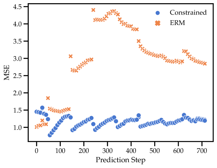
Figure 1: Test Mean Squared Error (MSE) computed at individual time steps on the forecasting window for Autoformer (Wu et al., 2021) on exchange rate data using ERM and our approach.

1 Introduction

Predicting multiple future values of time series data, also known as multi-step forecasting (Bontempi et al., 2013), has a myriad of applications such as weather (Wang et al., 2016), demand (Yi et al., 2022), price (Chen et al., 2018) and movility (Bai et al., 2019) forecasting. Several approaches to generating predictions for the next window have been proposed, including direct (Chevillon, 2007; Sorjamaa et al., 2007), autoregressive or recursive (Hill et al., 1996; Tiao & Tsay, 1994; Hamzaebi et al., 2009) and MIMO (Kline, 2004; Bontempi, 2008; Bontempi & Ben Taieb, 2011; Kitaev et al., 2019; Zhou et al., 2021; Wu et al., 2021; Liu et al., 2021; Zhou et al., 2022; Nie et al., 2022; Zeng et al., 2023; Garza & Mergenthaler-Canseco, 2023; Das et al., 2023b) techniques. Moreover, a plethora of learning parametrizations exist, ranging from linear models (Box & Jenkins, 1976; Zeng et al., 2023) to recent transformer architectures (Kitaev et al., 2019; Zhou et al., 2021; Wu et al., 2021; Liu et al., 2021; Zhou et al., 2022; Nie et al., 2022; Garza & Mergenthaler-Canseco, 2023; Das et al., 2023b).

Regardless of the model and parametrization, most approaches optimize a performance, risk or model fit functional (usually MSE), averaged over the predicted window. Therefore, the distribution of errors across the window – without any additional assumptions – can vary depending on the model and data generating process. In practice, this can lead to uneven performance across the different steps of the window.

Recent works using transformer based architectures focus on aggregate metrics, see for example (Kitaev et al., 2019; Wu et al., 2021; Nie et al., 2022), while addressing errors at different time steps has recieved little attention (Cheng et al., 2023). Our first contribution is providing an empirical analysis in this direction:

• We provide an empirical analysis of the distribution of errors across the prediction windows using popular models (Kitaev et al., 2019; Zhou et al., 2021; Wu et al., 2021) as well as a vanilla transformer in common benchmark datasets.

The analysis in (C1) gives evidence supporting that loss landscapes vary considerably between datasets and architectures. However, having no control on the error incurred at each time step in the predicted window can be detrimental in scenarios that can be affected by this variability. For example, analysing average behaviour is insufficient to assess financial risks in econometrics  (Chavleishvili & Manganelli, 2019) or to ensure stability when using the predictor in a Model Predictive Control framework (Terzi et al., 2021).

Therefore, our second contribution is addressing this problem through constrained learning.

• We formulate multi-step series forecasting as a constrained learning problem, which aims to find the best model in terms of average performance while imposing a user-defined upper bound on the loss at each time-step.

Since this constrains the distribution of the loss per time step across the window, we call this approach loss shaping constraints. Due to the challenges in finding appropriate constraints, we leverage a recent approach (Hounie et al., 2023) to re-interpret the specification as a soft constraint and find an optimal relaxation while jointly solving the learning task. We leverage recent duality results (Chamon & Ribeiro, 2020) to show that, despite being non-convex, the resulting problem has a bounded duality gap. This allows us to provide approximation guarantees at the step level.

We then propose an alternating Primal-Dual algorithm to tackle the loss shaping constrained problem. Our final contribution is the experimental evaluation of this algorithms in a practical setting:

• We evaluate our algorithms for different constraints using state-of-the-art transformer architectures (Kitaev et al., 2019; Zhou et al., 2021; Wu et al., 2021) in popular forecasting benchmarks.

Our empirical results showcase the ability to alter the shape of the loss by introducing constraints, and how this can lead to better performance in terms of standard deviation across the predictive window.

1.1 Related work

There is little prior work in time series prediction on promoting or imposing a certain distribution of errors across the predicted window, i.e., at specific timesteps. Works that propose reweighting the errors at different steps of the window mostly aim to improve average performance by leveraging the structure of residuals (Chevillon, 2007; Guo et al., 1999; Hansen, 2010) and rely on properties of the data generating process and predictive model class. On the other hand, works that address the empirical distribution of forecasting errors and robustness in non-parametric models (Spiliotis et al., 2019; Taleb, 2009) do not analyse the distribution of errors across multiple steps. Similarly, Multiple output Support Vector Regression for multi-step forecasting (Bao et al., 2014), which also tackles a constrained problem, has only addressed aggregate errors across the whole window.

In the context of transformer architectures for time series forecasting, to the best of our knowledge, loss at the step level has only been reported in (Cheng et al., 2023). Since the focus of the analysis is portraying the effect of a multi task learning approach on loss imbalance, the number of models and datasets for which step-wise errors across the window are reported is limited. Thus, it does not allow comparisons across datasets and models, and does not uncover the erratic (and non monotonic) behaviour that we have found empirically for some datasets and models. Recent works in generative time series models have also sought to impose constraints using penalty based methods (Coletta et al., 2023), but the nature of the constraints and proposed approach also differs from ours.

2 Multi-Step Time Series Forecasting

Let $\mathbf{x}_{t}\in\mathcal{X}\subseteq\mathbb{R}^{d_{x}}$ denote the in feature vector and $y_{t}\in\mathcal{Y}\subseteq\mathbb{R}^{d_{y}}$ its associated output or measurement at time step $t$. The goal in multi-step time series forecasting is to predict $T_{p}$ future values of the output, i.e., $y_{p}:=y_{[t+1:t+T_{p}]}$ given a window of length $T_{c}$ of input features, i.e., $\mathbf{x}_{c}:=\mathbf{x}_{[t-T_{c}:t]}$. The quality of the forecasts can be evaluated at each time-step using a non-negative loss function or metric $\ell:\mathcal{Y}\times\mathcal{Y}\to\mathbb{R}_{+}$, e.g., the squared error or absolute difference.

The most common approach in supervised multi-step forecasting is to learn a predictor that minimizes the expected loss averaged over the predicted window:

$$~{}\operatorname{min.}_{\boldsymbol{\theta}\in\Theta}\quad\mathbb{E}_{(\mathbf{x}_{c},y_{p})\sim\mathfrak{D}}\left[\frac{1}{T_{p}}\sum_{i=1}^{T_{p}}\ell_{i}({f_{\boldsymbol{\theta}}(\mathbf{x}_{c})},y_{p})\right],$$ (ERM)

where $\ell_{i}:=\ell({[f_{\boldsymbol{\theta}}(\mathbf{x}_{c})}]_{i},[y_{p}]_{i})$ denotes the loss evaluated at the $i$-th time step, $\mathfrak{D}$ a probability distribution over data pairs ${(\mathbf{x}_{c},y_{p})}$ and ${f_{\boldsymbol{\theta}}:\mathcal{X}^{T_{c}}\to\mathcal{Y}^{T_{p}}}$ is a predictor associated with parameters $\boldsymbol{\theta}\in\Theta\subset\mathbb{R}^{k}$, for example, a transformer based neural network architecture.

However, this choice of objective does not account for the structure or distribution of the errors across different time steps, which can lead to disparate behaviour across the predicted window as depicted in Figure 1. In particular, we observe empirically that state-of-the-art transformer architectures (Kitaev et al., 2019; Zhou et al., 2021; Wu et al., 2021) can yield highly varying loss dynamics, including non-monotonic, flat and highly non-linear landscapes, as presented in Section 5.1.

In order to control or promote a desirable loss pattern, a weighted average across time steps could be employed. However, since the realised losses will depend not only on the data distribution but also on the model class and learning algorithm. As a result, such penalization coefficients would have to be tuned in order to achieve a desired loss pattern, which in contrast can be naturally expressed as a requirement, as presented next.

3 Loss Shaping Constraints

In order to control the shape of the loss over the time window, we require the loss on timestep $i$ to be smaller than some quantity $\boldsymbol{\epsilon}_{i}$. This leads to the constrained statistical learning problem:

An advantage of (3) is that it is interpretable in the sense that constraints – unlike penalty coefficients – make explicit the requirement that they represent. That is, the constraint is expressed of terms of the expected loss at individual time-steps, and thus prior knowledge about and the underlying data distribution and model class can be exploited.

In Section 5, we focus on simply imposing a constant upper bound for all time steps, which we set using the performance of the (unconstrained) ERM solution. By upper bounding the error, we prevent errors from being undesirably large irrespectively of their position in the window, effectively limiting the spread of the errors across the whole window. Since we still minimize the mean error across the window, this approach is not as conservative as minimax formulations (Liu & Taniguchi, 2021), which only focus on the worst error.

It is worth pointing out that many other constraint choices are possible. For instance, it is often reasonable to assume errors increase monotonically along the prediction window. In this case, $\boldsymbol{\epsilon}_{i}$ could take increasing values based on prior knowledge of the learning problem. We provide further discussions about such configurations in Appendix B.1.

Nonetheless, which loss patterns are desirable and attainable will depend ultimately on the model, data and task at hand. In the next section we explore how to automatically adapt constraints during training, so that the problem is more robust to their mis-specification.

3.1 Adapting Constraints: A Resilient Approach.

An important challenge is the specification of loss shaping constraints that are not overly restrictive and make the problem feasible. Whereas in unconstrained average risk minimization (ERM) an optimal function $\theta^{\star}$ always exists, in (3) there may be no parameters in $\Theta$ satisfy the requirements. In practice, landing on satisfiable loss shaping requirements may necessitate the relaxation of some constraints –i.e., the values of $\boldsymbol{\epsilon}_{i}$ in (3)–. This is challenging because assessing the impact of tightening or relaxing a particular constraint can have intricate dependencies with the model class, the unknown data distribution, and learning algorithm, which are hard to determine a priori. Thus, the point at issue is coming up with reasonable constraints that achieve a desirable trade-off between controlling the distribution of the error across the predictive window and attaining good average performance. That is, for larger constraint levels the average performance improves, although the constraints will have less impact on the optimal function $f_{\theta^{\star}}$.

In order to do so, we introduce a non negative perturbation $\boldsymbol{\zeta}_{t}\in\mathbb{R}_{+}$ associated to each time step, and consider relaxing the $i-th$ constraint in the original problem by $\boldsymbol{\zeta}_{i}$. Explicitly, we impose $\mathbb{E}_{(\mathbf{x}_{c},y_{p})\sim\mathfrak{D}}\left[\ell_{i}({f_{\boldsymbol{\theta}}(\mathbf{x}_{c})},y_{p})\right]\leq\boldsymbol{\epsilon}_{i}+\boldsymbol{\zeta}_{i}$. We also introduce a differentiable, convex, non-decreasing cost $h:\mathbb{R}_{+}^{T_{p}}\to\mathbb{R}_{+}$, that penalizes deviating from the original specification, e.g., the squared $L_{2}$ norm $h(\boldsymbol{\zeta})\propto\|\boldsymbol{\zeta}\|_{2}^{2}$.

This allow us to re-interpret the initial constraint levels $\boldsymbol{\epsilon}$ as a soft constraint and use the perturbation cost $h$ to search for a perturbation $\zeta$ that achieves a good trade-off with average performance. Therefore, we propose to solve a Resilient Constrained Learning problem (Hounie et al., 2023), which is defined as follows:

The key property of the optimal relaxation $\boldsymbol{\zeta}^{\star}$ is that it equates the marginal cost of the relaxation (as measured by $h$) with the marginal cost of its effect on the optimal cost (Hounie et al., 2023). The rationale behind introducing a learnt relaxation of constraint levels is making the problem easier to solve. In the next section, we introduce practical primal-dual algorithms that enable approximating the constrained (3) and resilient (3.1) problems based on samples and finite (possibly non-convex) parametrizations such as transformer architectures.

4 Empirical Dual Resilient and Constrained Learning

A challenge in solving (3) and (3.1) is that in general, (i) no closed form projection into the feasible set or proximal operator exists, and (ii) it involves an unknown data distribution $\mathfrak{D}$. In what follows, we describe our approach for tackling the Resilient problem, noting that Primal-Dual algorithms tackling the original constrained problem can be similarly derived by simply excluding the slack variables.

To undertake 3.1, (i) we replace expectations by sample means over a data set $\{(\boldsymbol{x}_{c}^{n},y_{p}^{n})\>:\>n=1,\cdots,N\}$, as typically done in (unconstrained) statistical learning, and (ii) resort to its Lagrangian dual.

These modifications lead to the Empirical Dual problem

$$~{}\hat{D}^{\star}= \max_{\boldsymbol{\lambda}\geq 0}\;\;\min_{\boldsymbol{\boldsymbol{\theta}}\in\Theta,\;\boldsymbol{\zeta}\in\mathbb{R}^{\tiny T_{p}}_{+}}\hat{L}(\boldsymbol{\boldsymbol{\theta}},\boldsymbol{\lambda},\mathbf{\boldsymbol{\epsilon}},\boldsymbol{\zeta}),$$ (ED-LS)

where $\hat{L}$ is the empirical Lagrangian of (3.1), defined as

$${\hfilneg\hat{L}(\boldsymbol{\boldsymbol{\theta}},\boldsymbol{\lambda},\boldsymbol{\epsilon},\boldsymbol{\zeta}):=\hskip 10000.0pt}$$

$$\frac{1}{N}\sum_{n=1}^{N}\sum_{i=1}^{T_{p}}\left(\boldsymbol{\lambda}_{i}+\frac{1}{T_{p}}\right)\left[\ell_{i}({[f_{\boldsymbol{\theta}}(\mathbf{x}_{c}^{n})]},y_{p}^{n})\right]-\boldsymbol{\lambda}_{i}(\boldsymbol{\epsilon}_{i}+\boldsymbol{\zeta}_{i}),$$

and $\boldsymbol{\lambda}_{i}$ is the dual variable associated to the constraint on the $i$-th time step loss $\ell_{i}$.

The Empirical Dual problem (ED-LS) is an approximation of the Dual problem associated to 3.1 based on training samples. The dual problem itself can be interpreted as finding the tightest lower bound on the primal. Although the estimation of expectations using sample means and non-convexity of the hypothesis class can introduce a duality gap, i.e., $\hat{D}^{\star}<P^{\star}$, under certain conditions this gap can be bounded.

Unlike unconstrained statistical learning bounds, these approximation bounds depend not only in the sample complexity of the model class and loss but also on the optimal dual variables or slacks associated to the constraint problem. These reflect how challenging it is to meet the constraints. This aspect is crucial, as applying overly stringent loss shaping constraints in a given learning setting may be detrimental in terms of approximation and lead to sub-optimal test performance. We include a summary of these results as well as a discussion on their implications in this setting in Appendix A, and refer to (Chamon & Ribeiro, 2020; Hounie et al., 2023) for further details.

The advantage of tackling the the empirical dual problem $\hat{D}^{\star}$ is that it can be solved using saddle point methods presented in the next section.

4.1 Algorithm

In order to solve problem (ED-LS), we resort to dual ascent methods, which can be shown to converge even if the inner minimization problem is non-convex (Chamon et al., 2022). The saddle point problem (ED-LS) can then be undertaken by alternating the minimization with respect to $\boldsymbol{\theta}$ and $\boldsymbol{\zeta}$ with the maximization with respect to $\boldsymbol{\lambda}$ (K. J. Arrow & Uzawa, 1960), which leads to the Primal-Dual constrained learning procedure in Algorithm 1.

Although a bounded empirical duality gap does not guarantee that the primal variables obtained after running Algorithm 1 are near optimal or approximately feasible in general, recent constrained learning literature provides sub-optimality and near-feasibility bounds for primal iterates (Elenter et al., 2024) as well as abundant empirical evidence (Robey et al., 2021; Gallego-Posada et al., 2022; Elenter et al., 2022) that good solutions can still be obtained.

Algorithm 1 Primal Dual Loss Shaping.

  Input: Dataset $\{x_{i},y_{i}\}_{i=1,\cdots,N}$, primal learning rate $\eta_{p}$, dual learning rate $\eta_{d}$, perturbation learning rate $\eta_{\epsilon}$, number of epochs $T_{e}$, number of batches $T_{b}$, initial constraint tightness $\epsilon_{\alpha_{0}}$.

  Initialize: $\boldsymbol{\theta},\lambda_{1},\dots,\lambda_{T_{\text{pred}}}\leftarrow\mathbf{0}$

  for $\text{epoch }=1,\ldots,T_{e}\>$ do

     for $\text{batch }=1,\ldots,T_{b}\>$ do

             Update primal variables

        $\boldsymbol{\theta}\leftarrow\boldsymbol{\theta}-\eta_{p}\nabla_{\theta}\hat{L}(\boldsymbol{\theta},\boldsymbol{\lambda},\boldsymbol{\epsilon},\boldsymbol{\zeta})$

             Evaluate constraints.

        $\mathbf{s}_{i}\leftarrow\left(\frac{1}{N_{b}}\sum_{n=1}^{N_{b}}\ell_{i}({[f_{\boldsymbol{\theta}}(\mathbf{x}_{\text{c}(t)}^{n})]},y_{\text{p}(t)}^{n})\right)-(\epsilon_{i}+\boldsymbol{\zeta}_{i})$

             Update slacks.

        $\boldsymbol{\zeta}\leftarrow\left[\boldsymbol{\zeta}-\eta_{\zeta}\Big{(}\nabla h\big{(}\boldsymbol{\zeta}\big{)}-\boldsymbol{\lambda}\Big{)}\right]_{+}$

             Update dual variables.

        $\boldsymbol{\lambda}\leftarrow\left[\lambda+\eta_{d}\mathbf{s}\right]_{+}$

     end for

  end for

  Return: $\boldsymbol{\theta}$, $\boldsymbol{\lambda}$.

5 Experiments

In order to explore the properties of loss shaping, we turn to the open source benchmark datasets Electricity Consuming Load (ECL), Weather  and Exchange (Lai et al., 2018) to train three popular transformer architectures for time series prediction, namely, Reformer (Kitaev et al., 2019) and Autoformer (Wu et al., 2021), Informer (Zhou et al., 2021) and a vanilla transformer. We contrast their behavior in constrained and (standard) unconstrained learning settings. We follow the same setup and hyperparameters used in (Kitaev et al., 2019; Wu et al., 2021; Zhou et al., 2021). Data is split into train, validation, and test chronologically with a ratio of 7:1:2. For each set every possible pair of consecutive context and prediction windows of length $T_{c}$ and $T_{p}$, respectively, are used. That is, we use rolling (overlapping) windows for both training and testing. We use ADAM optimizer (Kingma & Ba, 2014) together with the original implementation and hyperparameters of each method. Additional experimental details can be found on Appendix C.

5.1 The Shape of ERM

In this section, we provide an empirical analysis of the distribution of errors across time steps when training models with the conventional ERM framework. This aims to uncover phenomena that cannot be inferred from the commonly reported metrics – which are averaged across the window – and to highlight that generalization may hinder the efficacy of loss shaping approaches.

Models For the same dataset and prediction length, different models can have significantly different error patterns, even when having similar MSEs. This can be observed in Figure 3, which portray the test errors of different models trained on the same datasets. This can also be seen in Table 4, which shows that the standard deviation of step-wise MSEs considerably, while their averages (Table 3) are similar.

Prediction Length We observe that the shape of the loss is similar across different prediction lengths in some settings, such as the one depicted in Figure 2. In Appendix C.1 we provide further quantitative evidence of this phenomenon by computing pairwise correlations between (scaled) errors from different prediction lengths.

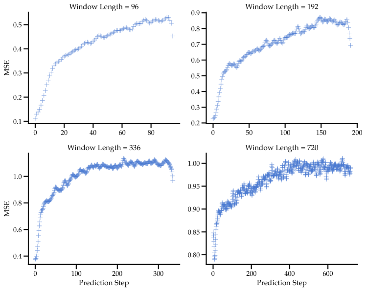
Figure 2: Step-wise Mean Test Errors for Autoformer on the Weather dataset. Each plot represents a different prediction length window. The shape of the error across the window is similar across prediction lengths.

Generalization In order to assess the impact of the generalization gap on the test error shape, we analyse whether at any given step smaller mean training errors are associated to smaller test errors. We compute for each model, dataset and prediction length, the Spearman correlation between mean stepwise errors computed on the training and test sets. As shown in Table 1, in several setups we find strong correlations, signaling a monotonic relationship between train and test errorsHowever, we also observe a number of weak and even negative correlations. In particular, Informer and the vanilla transformer, present significantly weaker correlations. In these settings, imposing a desired loss shape by modifying the distribution of errors on the training set can be challenging, because it need not affect performance on the test set in a predictable manner.

		Autoformer	Informer	Reformer	Transformer
ECL	96	0.60	0.28	0.91	-0.05
	192	0.93	0.14	0.67	0.05
	336	-0.09	0.31	0.38	0.10
	720	0.75	0.05	0.30	0.09
Exchange	96	0.94	0.34	0.91	-0.04
	192	0.64	-0.00	-0.36	-0.81
	336	0.90	0.07	-0.58	-0.31
	720	0.99	0.40	-0.28	-0.42
Weather	96	-0.28	0.80	0.97	-0.33
	192	0.98	0.43	0.95	0.08
	336	0.95	0.26	0.87	0.26
	720	0.82	0.21	0.68	0.10

Table 1: Spearman Correlations between train and test errors for models trained using ERM. Higher means the relationship is closer to being monotonic.

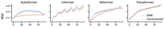
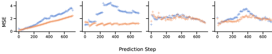
Figure 3: Test MSE computed at each prediction step for different datasets, models and prediction window lengths. The top row shows results for the weather dataset with a predictive window length of 96 steps, and the second row corresponds to the exchange dataset with a predictive window length of 720 steps. Each plot corresponds to a different architecture, and each curve represents a different training algorithm, we include both the ERM baseline and our method using a constant constraint across the window for all models.

5.2 Constraint Level Choice

The most salient design question is the choice of the constraint level $\boldsymbol{\epsilon}_{i}$. In our experimental setting, we begin with the simplest choice of a constant $\boldsymbol{\epsilon}_{i}=\boldsymbol{\epsilon}$ for all timesteps.

The value of $\boldsymbol{\epsilon}$ should depend on the statistical problem at hand, that is, the model class, loss and data distribution. It will also depend on the sample size since, even if the model has enough capacity to fit an extremely tight constraint, it can overfit to training data while being infeasible at test time. On the other hand, if the constraint level is too loose it will not significantly modify the shape of the loss across the window. Lacking prior information or domain knowledge, we propose using the train and validation loss (see Appendix C) of a model trained using ERM in order to gather insights about sensible values of $\boldsymbol{\epsilon}$.

During preliminary experiments, we observed that the median of the ERM validation loss per time step achieved good results. We also conducted an ablation on constraint levels using the upper and lower quantiles of train and validation losses (see Appendix C.1). We report the results on the values of $\boldsymbol{\epsilon}$ with the lower MSE for each combination of model, dataset and prediction length.

In order to quantify the effect of the imposed constraints, we report Mean Constraint Violation (MCV), which we define as the fraction of time-steps that are infeasible, explicitly,

$$\mathcal{MCV}(\hat{y},y,\boldsymbol{\epsilon})=\frac{1}{T_{pred}}\sum^{T_{pred}}_{t=1}\mathrm{max}\{0,\ell(\hat{y}_{t},y_{t})-\boldsymbol{\epsilon}\}.$$

An effective constrained model should be able to marginally trade-off MSE for a significant reduction in MCV.

5.3 Constrained Loss Shaping Results

		Autoformer			Informer			Reformer			Transformer
		Ours	Ours+R	ERM	Ours	Ours+R	ERM	Ours	Ours+R	ERM	Ours	Ours+R	ERM
ECL	96	0.087	0.109	0.091	0.170	0.193	0.176	0.147	0.152	0.149	0.149	0.169	0.152
	192	0.026	0.056	0.017	0.173	0.192	0.184	0.166	0.172	0.172	0.063	0.110	0.070
	336	0.042	0.080	0.127	0.159	0.174	0.165	0.198	0.162	0.192	0.157	0.168	0.150
	720	0.093	0.227	0.075	0.165	0.226	0.173	0.139	0.148	0.139	0.155	0.173	0.151
Exchange	96	0.022	0.006	0.015	0.834	0.872	0.842	0.917	0.873	0.852	0.008	0.003	0.084
	192	0.000	0.000	0.791	1.068	1.089	1.071	1.213	1.496	1.209	1.218	1.139	1.200
	336	0.000	0.000	2.411	0.000	0.000	0.000	1.423	1.715	1.700	1.323	1.610	1.382
	720	0.778	0.382	1.160	0.000	0.000	0.000	1.460	1.506	1.492	0.000	0.000	0.156
Weather	96	0.000	0.000	0.000	0.186	0.230	0.225	0.000	0.019	0.000	0.047	0.030	0.040
	192	0.001	0.001	0.002	0.019	0.040	0.045	0.000	0.018	0.129	0.411	0.458	0.485
	336	0.018	0.002	0.013	0.411	0.355	0.355	0.010	0.040	0.289	0.209	0.218	0.086
	720	0.000	0.000	0.000	0.802	0.949	0.851	0.478	0.631	0.680	0.708	0.856	0.786

Table 2: Test Mean Constraint Violation using constant constraints and vanilla ERM models across different window lengths. Imposing constraints consistently reduces the MCV metric across datasets and window lengths.

		Autoformer			Informer			Reformer			Transformer
		Ours	Ours+R	ERM	Ours	Ours+R	ERM	Ours	Ours+R	ERM	Ours	Ours+R	ERM
ECL	96	0.200	0.220	0.204	0.319	0.342	0.325	0.297	0.303	0.299	0.259	0.278	0.262
	192	0.226	0.258	0.215	0.341	0.360	0.352	0.326	0.332	0.332	0.274	0.321	0.281
	336	0.249	0.287	0.334	0.348	0.371	0.354	0.365	0.329	0.359	0.287	0.297	0.280
	720	0.270	0.410	0.252	0.377	0.438	0.385	0.316	0.326	0.316	0.293	0.312	0.289
Exchange	96	0.179	0.163	0.155	0.872	0.910	0.880	1.025	0.981	0.960	0.593	0.556	0.691
	192	0.266	0.267	2.052	1.110	1.131	1.113	1.402	1.685	1.398	1.253	1.174	1.235
	336	0.446	0.442	3.442	1.088	1.080	1.633	1.632	1.924	1.909	1.362	1.649	1.421
	720	1.510	1.205	1.852	1.170	1.166	2.961	2.063	2.114	2.095	1.029	1.015	2.197
Weather	96	0.300	0.314	0.375	0.395	0.441	0.435	0.361	0.380	0.422	0.462	0.435	0.448
	192	0.311	0.322	0.303	0.447	0.491	0.515	0.425	0.483	0.703	0.593	0.640	0.667
	336	0.374	0.402	0.359	0.656	0.600	0.600	0.589	0.655	1.010	0.901	0.915	0.749
	720	0.442	0.447	0.443	1.051	1.198	1.100	0.761	0.914	0.963	0.924	1.072	1.002

Table 3: Test MSE for constrained and ERM models across different window lengths. We observe that the tradeoff between constraint satisfaction and MSE is low, even improving MSE in many instances.

		Autoformer			Informer			Reformer			Transformer
		Ours	Ours+R	ERM	Ours	Ours+R	ERM	Ours	Ours+R	ERM	Ours	Ours+R	ERM
ECL	96	0.015	0.013	0.015	0.013	0.018	0.014	0.011	0.008	0.011	0.007	0.008	0.007
	192	0.022	0.020	0.022	0.037	0.029	0.041	0.019	0.012	0.020	0.018	0.014	0.018
	336	0.019	0.063	0.043	0.018	0.019	0.022	0.023	0.011	0.022	0.022	0.018	0.020
	720	0.030	0.156	0.035	0.020	0.040	0.028	0.007	0.007	0.007	0.018	0.018	0.013
Exchange	96	0.084	0.061	0.080	0.274	0.305	0.278	0.121	0.098	0.115	0.162	0.128	0.167
	192	0.447	0.389	1.347	0.299	0.331	0.308	0.148	0.196	0.132	0.375	0.374	0.376
	336	9.441	0.843	2.132	0.392	0.376	0.387	0.172	0.269	0.193	0.211	0.304	0.218
	720	0.226	0.422	1.038	0.915	1.093	0.946	0.280	0.344	0.314	0.624	0.735	0.610
Weather	96	0.029	0.026	0.060	0.141	0.096	0.118	0.107	0.090	0.101	0.121	0.124	0.126
	192	0.069	0.040	0.052	0.156	0.127	0.158	0.144	0.132	0.142	0.206	0.242	0.242
	336	0.037	0.067	0.068	0.124	0.171	0.136	0.035	0.191	0.141	0.252	0.262	0.224
	720	0.081	0.065	0.079	0.251	0.528	0.364	0.038	0.067	0.039	0.273	0.324	0.289

Table 4: Standard deviation of stepwise errors for runs with $\boldsymbol{\epsilon}$ set to the Median of train Error for ERM. “Ours” denotes the constrained approach and “Ours(R)” adds a resilient relaxation with cost $h(\boldsymbol{\zeta})=2\|{\boldsymbol{\zeta}\|}_{2}^{2}$. Imposing constraints tends to reduce the variance across the predictive window. Adding resilience often achieves even less variability, especially in cases where the STD of constrained methods is high.

Our approach effectively affects the distribution of losses across the window as intended in many cases, although it fails to do so in others, as depicted in Figure 3 and Appendix C.1. Nonetheless, we corroborate empirically that it consistently reduces constraint violation (shown in Table 2) on test data across different transformer-based architectures, prediction lengths and datasets.

Furthermore, this does not come at a cost in terms of test MSE (Table 3), which is similar between ERM and our approach in most scenarios. In several settings, our approach even leads to a reduction in MSE. For example, this effect is illustrated in Figure 3, where the Autoformer model trained with constraints attains a smoother error landscape, with most step-wise errors being lower than their ERM counterpart.

The rationale behind imposing an upper bound at each step is reducing the spread of errors across the windows. In Table 4 we show that the standard deviation (computed across the predicted window) is reduced for the vast majority of settings – with the exception of the vanilla transformer, that as already discussed shows poor generalization –. In addition, in Appendix C.1 we provide examples in which the loss landscape in unseen data changes even when imposing looser constraints that are easily satisfied over the training set – i.e., for which the ERM solution is also feasible–. This suggests that irrespective of the level of constraint imposed, using constraints can contribute to enhancing model performance.

Qualitatively, we can distinguish different scenarios in which our approach leads to improvements. On some settings, it can make training errors feasible possibly at the cost of an increase of average training error (e.g., the first row of Figure 4). Conversely, in other scenarios, it fails to obtain a feasible solution and leads to an increase training error, but still improves test performance due to better generalization, like in the second row of Figure 4.

Among the settings in which we are unable to change the test loss as desired, we also distinguish two common failure modes. The first is when our approach fails to impose the constraints on training data, as in the first row of Figure 5, often associated with more challenging settings. Another one is the lack of generalization, depicted in the second row of Figure 5, which corresponds to settings in which our model effectively changes the loss pattern in the training set, but it does not have the same effect on test data.

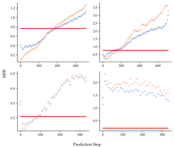
Figure 4: Examples of success cases. The first row corresponds to the training and testing losses of ERM and Constrained Autoformer on Exchange Rate data, with window length of 720. The second row is Reformer on Exchange Rate with window length of 336. The red lines are the values of $\boldsymbol{\epsilon}$ used during training.

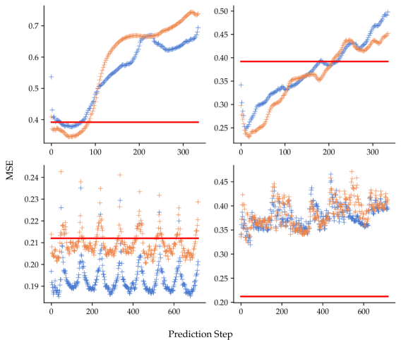
Figure 5: Two instances of failure cases. The first row is the training and testing errors of Autoformer on Weather data with window length of 336. The second row is Informer on ECL data with window length of 720. The red lines are the values of $\boldsymbol{\epsilon}$ used during training.

5.4 Resilience

Relaxing constraints should allow for a better average performance (objective), in the same way that imposing constraints should only cause a decrease performance when compared to the unconstrained problem. In the previous section, we have shown that – empirically – the latter does not always hold. In the same manner, the Resilient approach did not consistently attain lower test MSEs (Table 3) than the constrained approach, even though constraints were effectively relaxed – by a considerable amount –. Settings in which relaxing constraints is detrimental to performance thus support the claim that loss shaping constraints can also be beneficial in terms of average MSE in some cases. Examples of this behavior can be observed in Figure 3 for the case of Autoformer and Informer.

In terms of constraint violation, which we measure with respect to the fixed constraint levels ($\boldsymbol{\epsilon}$), the resilient approach should be outperformed by its constrained counterpart. However, we find that both approaches perform similarly.

Finally, we observe that the resilient approach can be advantageous in that it reduces standard deviation (Table 4) across the window considerably in many cases. For example, this can be observed for Autoformer (first columns) across several settings.

6 Conclusion

This paper introduced a time series forecasting constrained learning framework that aims to find the best model in terms of average performance while imposing a user defined upper bound on the loss at each time-step. Given that we observed that the distribution of loss landscapes varies considerably, we explored a Resilient Constrained Learning (Hounie et al., 2023) approach to dynamically adapt individual constraints during training. We analysed the properties of this problem by leveraging recent duality results, and developed practical algorithms to tackle it. We corroborated empirically that our approach can effectively alter the distribution of the loss across the forecast window.

Although we have focused on transformers for long term time series forecasting, motivated by the empirical finding that their loss varies considerably, the loss shaping constrained learning framework can be extended to other settings. This includes a plethora of models, datasets and tasks where losses are distributed across different time steps or grids.

Appendix A Approximation Guarantees

The functional space induced by the parametrization, which we will denote $\mathcal{F}_{\theta}=\{f_{\theta}:\boldsymbol{\theta}\in\Theta\}$ can be non-convex, as in the case of transformer architectures. However, it has been shown (Chamon & Ribeiro, 2020; Hounie et al., 2023) that as long as the distance to its convex hull $\overline{\mathcal{F}}_{\theta}=\operatorname{conv}({\mathcal{F}}_{\theta})$ is bounded, then we can leverage the strong duality of the convex variational program defined over $\overline{\mathcal{F}}_{\theta}$ together with uniform convergence bounds to provide approximation guarantees. That is, the values of (3.1) and (ED-LS) are close. This holds both for the constrained and resilient formulation, although as discussed next, the resilient problem requires milder assumptions.

Assumption A.1.

There exist a function $\phi\in\mathcal{F}$ such that all constraints are met with margin $c>0$, i.e., ${\mathbb{E}}_{\mathcal{D}_{i}}\big{[}\ell_{i}(\phi({\mathbf{x}}),y)\big{]}\leq c$, for all $i=1,\dots,m$.

Assumption A.1${.^{\prime}}$ There exist a finite relaxation $\boldsymbol{\zeta}\preceq\infty$ and a function $\phi\in\mathcal{F}$ such that all constraints are met with margin $c>0$, i.e., ${\mathbb{E}}_{\mathcal{D}_{i}}\big{[}\ell_{i}(\phi({\mathbf{x}}),y)\big{]}\leq\boldsymbol{\zeta}-c$, for all $i=1,\dots,m$.

Assumption A.2.

The loss functions $\ell_{i}$, $i=0\dots m$, are convex and $M$-Lipschitz continuous.

Assumption A.3.

For every $\phi\in\mathcal{F}$, there exists $\boldsymbol{\theta}^{\dagger}\in\Theta$ such that ${\mathbb{E}}_{\mathcal{D}_{i}}\big{[}|\phi({\mathbf{x}})-f_{\boldsymbol{\theta}^{\dagger}}({\mathbf{x}})|\big{]}\leq\nu$, for all $i=0,\dots,m$.

Assumption A.4.

There exists $\xi(N,\delta)\geq 0$ such that for all $i=0,\dots,m$ and all $\boldsymbol{\theta}\in\Theta$,

$$\bigg{|}{\mathbb{E}}_{\mathcal{D}_{i}}\big{[}\ell_{i}(f_{\theta}({\mathbf{x}}_{c}),y_{p})\big{]}-\frac{1}{N}\sum_{n=1}^{N}\ell_{i}\big{(}f_{\theta}({\mathbf{x}}_{c}^{n}),y_{p}^{n}\big{)}\bigg{|}\leq\xi(N,\delta)$$

with probability $1-\delta$ over draws of $\{({\mathbf{x}}_{i}^{n},y_{i}^{n})\}$.

Note that the constraint qualification in Assumption A.1 (known as Slater’s condition (Boyd et al., 2004)), which is required for the constrained problem, can be relaxed to the milder qualification given in Assumption A.1${.^{\prime}}$ for the resilient problem.

Assumption A.2 holds for commonly used objectives in Time-Series forecasting, including Mean Squared Error, Mean Absolute Error and Huber-loss, among others.

Assumption A.3 will hold if the parametrized function space is rich in the sense that the distance to its convex hull is bounded. Since neural networks and transformers have universal approximation properties (Hornik et al., 1989; Yun et al., 2019), we posit that given a parametrization with enough capacity, this assumption holds.

Assumption A.4 – known as uniform convergence – is customary in statistical learning theory. This includes generalization bounds based on VC dimension, Rademacher complexity, or algorithmic stability, among others (Mohri et al., 2018). Unlike generalization bounds for the unconstrained problem (ERM), this assumption bounds the loss at each step, and not the aggregated loss throughout the window.

We now state the main theorems that bound the approximation errors.

Theorem 1 (Hounie et al., 2023) Let $\boldsymbol{\zeta}^{\star}$ be an optimal relaxation for problem (3.1). Under Ass. A.1^′–A.4, it holds with probability of $1-(3m+2)\delta$ that

$$\big{|}P^{\star}-D^{\star}\big{|}\leq h(\boldsymbol{\zeta}^{\star}+1\cdot M\nu)-h(\boldsymbol{\zeta}^{\star})+M\nu+(1+\Delta)\xi(N,\delta)\text{.}$$

Theorem 2 (Chamon & Ribeiro, 2020) Let $\boldsymbol{\lambda}^{\star}$ be an optimal relaxation for the constrained problem (3) defined over $\overline{\mathcal{F}}_{\theta}$ with constraints $\boldsymbol{\epsilon}_{i}-M\nu$. Under Ass. A.1–A.4, it holds with probability of $1-(3m+2)\delta$ that

$$\big{|}P^{\star}-D^{\star}\big{|}\leq(1+\boldsymbol{\lambda}^{\star})M\nu+(1+\Delta)\xi(N,\delta)\text{.}$$

Note that unlike in unconstrained statistical learning, optimal dual variables $\boldsymbol{\lambda}^{\star}$ or relaxations $\boldsymbol{\zeta}^{\star}$ play an important role in these approximation bounds. This is because, intuitively, they represent the difficulty of satisfying constraints.

Appendix B Monotonic Loss constraints

A less restrictive constraint that accounts for error compounding is to only require errors to be monotonically increasing. That is, that there exists some $\boldsymbol{\epsilon}$ such that $\boldsymbol{\epsilon}_{t+1}\geq\boldsymbol{\epsilon}_{t}$ for all $t$. Instead of searching for such an $\boldsymbol{\epsilon}$, we can directly impose monotonicity, which requires only a small modification in  (3), as discussed in Section B.1.

B.1 Formulation

We can require the loss on each timestep $i$ to be smaller than the loss step at the following $i+1$. This leads to the constrained statistical learning problem:

Because of linearity of the expectation, the constraint can be re-written as a single expectation of a (non-convex) functional, explicitly,

$$\mathbb{E}_{(\mathbf{x}_{c},y_{p})\sim\mathfrak{D}} \left[\ell_{i}({f_{\boldsymbol{\theta}}(\mathbf{x}_{c})},y_{p})\right.$$

$$\quad\quad\quad\left.-\ell_{i+1}({f_{\boldsymbol{\theta}}(\mathbf{x}_{c})},y_{p})\right]\leq 0.$$

Despite the lack of convexity, the bounds presented in Appendix A still hold under additional assumptions on the distribution of the data and model class, as shown in Theorem 1 and Proposition B.1 (Chamon et al., 2022). We include these assumptions here for completeness.

Assumption B.1.

The functions $y\mapsto\ell_{i}(\phi(\cdot),y)f_{i}(\cdot\mid y),i=$ $1,\ldots,m$, are uniformly continuous in the total variation topology for each $\phi\in\mathcal{\mathcal{H}}$, where $f_{i}(\boldsymbol{x}\mid y)$ denotes the density of the conditional random variable induced by $\mathfrak{D}_{i}$. Explicitly, for each $\phi\in\overline{\mathcal{H}}$ and every $\epsilon>0$ there exists $\delta_{\phi,i}>0$ such that for all $|y-\tilde{y}|\leq\delta_{\phi,i}$ it holds that

$$\sup_{\mathcal{Z}\in\mathcal{B}}\int_{\mathcal{Z}}\left|\ell_{i}(\phi(\boldsymbol{x}),y)f_{i}(\boldsymbol{x}\mid y)-\ell_{i}(\phi(\boldsymbol{x}),\tilde{y})f_{i}(\boldsymbol{x}\mid\tilde{y})\right|d\boldsymbol{x}\leq\epsilon$$

Assumption B.2.

The conditional distribution $\boldsymbol{x}\mid y$ induced by $\mathfrak{D}$ are non-atomic.

Note that the epigraph formulation of (B.1) resembles that of the original los schaping constrained problem (3), with the difference that $\boldsymbol{\epsilon}$ is an optimization variable, now constrained to be monotonically increasing:

$$\min_{\boldsymbol{\theta}\in\Theta}\;\mathbb{E}_{(\mathbf{x}_{c},y_{p})\sim\mathfrak{D}}\left[\frac{1}{T_{p}}\sum_{i=1}^{T_{p}}\ell_{i}({f_{\boldsymbol{\theta}}(\mathbf{x}_{c})},y_{p})\right]$$

$$\text{s. to :}\quad\mathbb{E}_{(\mathbf{x}_{c},y_{p})\sim\mathfrak{D}}\left[\ell_{i}({f_{\boldsymbol{\theta}}(\mathbf{x}_{c})},y_{p})\right]\leq\boldsymbol{\epsilon}_{i}\;$$

$$\quad\quad\quad\quad\quad\quad\quad\quad\boldsymbol{\epsilon}_{i}\leq\boldsymbol{\epsilon}_{i+1}$$

$$\quad\quad\quad\quad\quad\quad\quad\quad i=1,\ldots,T_{p}-1.$$ (P-M-epi)

Appendix C Experiment Setup

Early Stopping While the common practice in transformers for forecasting is to train with early stopping, we disable it for the constrained approach and train for a full 10 epochs, due to the slower convergence. Note that in the results presented in this work we keep early stopping for ERM.

Tuning of dual learning rate and initialization parameters. Preliminary exploration yielded consistently superior results with dual learning rate set to 0.01 and duals initialized to 1.0. All experiments reported in the paper were performed with this parameterization.

Choice of $\boldsymbol{\epsilon}$. To choose an appropriate upper bound constraint for the stepwise losses, we perform a grid search of six values for every setting of dataset, model and prediction window, optimizing for validation MSE. The values for the search are the 25, 50, and 75th percentile of the training and validation errors of each model trained with ERM. The values reported in Tables 3 and 2 are for the optimal values of this grid search.

Alternative choices of epsilon. During preliminary experiments, we explored

C.1 Extended experiment results

		Autoformer	Informer	Reformer	Transformer
ECL	96	0.38	0.34	0.60	0.18
	192	0.42	0.17	0.37	-0.06
	336	0.17	0.17	-0.19	-0.16
	720	0.30	0.20	0.07	0.19
Exchange	96	0.76	0.20	0.67	-0.15
	192	0.32	0.08	0.19	-0.55
	336	0.24	-0.44	0.17	0.43
	720	0.69	-0.63	0.12	-0.69
Weather	96	0.01	0.23	0.14	-0.30
	192	0.43	-0.08	-0.43	0.33
	336	0.46	-0.22	0.55	0.25
	720	0.83	0.45	0.69	0.64

Table 5: Spearman correlation for step-wise Mean Train and Test errors, for models trained with constant constraints.

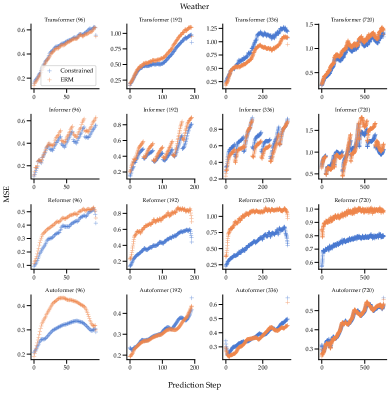
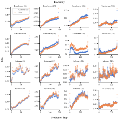
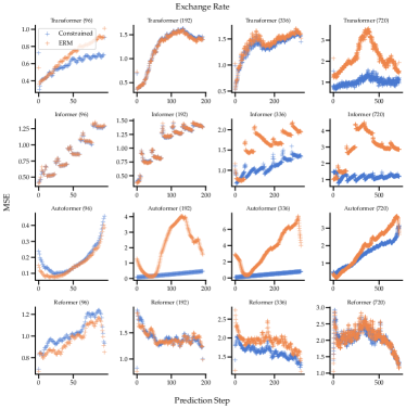
Figure 6: Full visualizations for the test loss landscapes of the Exchange, Weather and ECL datasets, on constrained and ERM losses.

C.1.1 Loss Shape Plots

Figure 6 shows the loss landscapes of the different transformer architectures tested on all three datasets. Some patterns in loss shapes across model architectures can be observed. For instance, Informer tends to have a jagged loss distribution with periodic discontinuities. On the other hand, Autoformer’s losses are concave or show seasonal patterns. These distributions could be due to the inherent inductive biases on each model architecture, such as the autocorrelation and trend decomposition mechanisms in Autoformer.

However, the particular shape of the loss remains idiosyncratic to each combination of dataset, model, and prediction window length. Furthermore, the effect of imposing constraints can be appreciated in multiple instances, where the constraints appear to have a corrective effect on extreme cases, improving MSE and MCV simultaneously.

Finally we also observe that, more often than not, loss landscapes are not linear, let alone constant. Moreover, in rare cases, such as Reformer on Exchange Rate with prediction window of 192 steps, the stepwise loss surprisingly trends downwards. This motivates further experimentation on different kinds of constraints that are better suited for a particular learning problem.

C.1.2 Correlation between training and test errors.

We compute the Spearman correlation between mean stepwise errors computed on the training and test sets for models trained with constant constraint levels. Compared to the values reported for ERM in Table 1, we observe weaker correlations for our method. This can indicate that, while imposing a constraint on the training loss, our approach increasingly overfits to training data.

C.1.3 Correlations between prediction lengths

In order to quantify the degree of similarity between error patterns across various prediction lengths, we compute Pearson correlation coefficients between step-wise errors, as shown in Figure 7. We achieve this by first re-sampling shorter prediction windows using linear interpolation to match the number of steps. Notably, some setups present high correlations for several prediction lengths, which we interpret as the error distributions being similar.

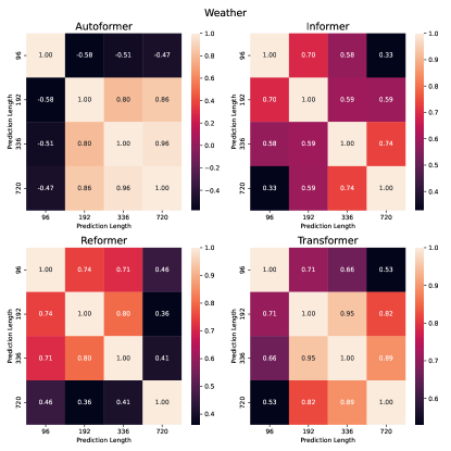
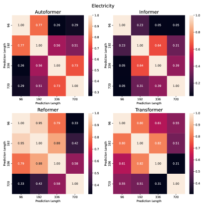
Figure 7: Pearson correlation between test step wise errors for weather and electricity datasets. Each heatmap shows pairwise correlations between all prediction lengths for a given model.

References

- Bai et al. (2019) Bai, L., Yao, L., Kanhere, S., Wang, X., Sheng, Q., et al. Stg2seq: Spatial-temporal graph to sequence model for multi-step passenger demand forecasting. arXiv preprint arXiv:1905.10069, 2019.
- Bao et al. (2014) Bao, Y., Xiong, T., and Hu, Z. Multi-step-ahead time series prediction using multiple-output support vector regression. Neurocomputing, 129:482–493, 2014.
- Bontempi (2008) Bontempi, G. Long term time series prediction with multi-input multi-output local learning. 2008. URL https://api.semanticscholar.org/CorpusID:137250.
- Bontempi & Ben Taieb (2011) Bontempi, G. and Ben Taieb, S. Conditionally dependent strategies for multiple-step-ahead prediction in local learning. International Journal of Forecasting, 27:689–699, 07 2011. doi: 10.1016/j.ijforecast.2010.09.004.
- Bontempi et al. (2013) Bontempi, G., Ben Taieb, S., and Le Borgne, Y.-A. Machine learning strategies for time series forecasting. Business Intelligence: Second European Summer School, eBISS 2012, Brussels, Belgium, July 15-21, 2012, Tutorial Lectures 2, pp. 62–77, 2013.
- Box & Jenkins (1976) Box, G. E. and Jenkins, G. M. Time series analysis. forecasting and control. Holden-Day Series in Time Series Analysis, 1976.
- Boyd et al. (2004) Boyd, S., Boyd, S. P., and Vandenberghe, L. Convex optimization. Cambridge university press, 2004.
- Chamon & Ribeiro (2020) Chamon, L. and Ribeiro, A. Probably approximately correct constrained learning. Advances in Neural Information Processing Systems, 33:16722–16735, 2020.
- Chamon et al. (2022) Chamon, L. F., Paternain, S., Calvo-Fullana, M., and Ribeiro, A. Constrained learning with non-convex losses. IEEE Transactions on Information Theory, 69(3):1739–1760, 2022.
- Chavleishvili & Manganelli (2019) Chavleishvili, S. and Manganelli, S. Forecasting and stress testing with quantile vector autoregression. Available at SSRN 3489065, 2019.
- Chen et al. (2018) Chen, Y., Zhang, C., He, K., and Zheng, A. Multi-step-ahead crude oil price forecasting using a hybrid grey wave model. Physica A: Statistical Mechanics and its Applications, 501:98–110, 2018.
- Cheng et al. (2023) Cheng, J., Huang, K., and Zheng, Z. Fitting imbalanced uncertainties in multi-output time series forecasting. ACM Transactions on Knowledge Discovery from Data, 17(7):1–23, 2023.
- Chevillon (2007) Chevillon, G. Direct multi-step estimation and forecasting. Journal of Economic Surveys, 21(4):746–785, 2007.
- Coletta et al. (2023) Coletta, A., Gopalakrishan, S., Borrajo, D., and Vyetrenko, S. On the constrained time-series generation problem. arXiv preprint arXiv:2307.01717, 2023.
- Das et al. (2023a) Das, A., Kong, W., Leach, A., Sen, R., and Yu, R. Long-term forecasting with tide: Time-series dense encoder. arXiv preprint arXiv:2304.08424, 2023a.
- Das et al. (2023b) Das, A., Kong, W., Sen, R., and Zhou, Y. A decoder-only foundation model for time-series forecasting, 2023b.
- Elenter et al. (2022) Elenter, J., Naderializadeh, N., and Ribeiro, A. A lagrangian duality approach to active learning. In Koyejo, S., Mohamed, S., Agarwal, A., Belgrave, D., Cho, K., and Oh, A. (eds.), Advances in Neural Information Processing Systems, volume 35, pp. 37575–37589. Curran Associates, Inc., 2022. URL https://proceedings.neurips.cc/paper_files/paper/2022/file/f475bdd151d8b5fa01215aeda925e75c-Paper-Conference.pdf.
- Elenter et al. (2024) Elenter, J., Chamon, L., and Ribeiro, A. Near-optimal solutions of constrained learning problems. In The Twelfth International Conference on Learning Representations, 2024. URL https://openreview.net/forum?id=fDaLmkdSKU.
- Gallego-Posada et al. (2022) Gallego-Posada, J., Ramirez, J., Erraqabi, A., Bengio, Y., and Lacoste-Julien, S. Controlled sparsity via constrained optimization or: How i learned to stop tuning penalties and love constraints. In Koyejo, S., Mohamed, S., Agarwal, A., Belgrave, D., Cho, K., and Oh, A. (eds.), Advances in Neural Information Processing Systems, volume 35, pp. 1253–1266. Curran Associates, Inc., 2022. URL https://proceedings.neurips.cc/paper_files/paper/2022/file/089b592cccfafdca8e0178e85b609f19-Paper-Conference.pdf.
- Garza & Mergenthaler-Canseco (2023) Garza, A. and Mergenthaler-Canseco, M. Timegpt-1. arXiv preprint arXiv:2310.03589, 2023.
- Guo et al. (1999) Guo, M., Bai, Z., and An, H. Z. Multi-step prediction for nonlinear autoregressive models based on empirical distributions. Statistica Sinica, 9(2):559–570, 1999. ISSN 10170405, 19968507. URL http://www.jstor.org/stable/24306598.
- Hamzaebi et al. (2009) Hamzaebi, C., Akay, D., and Kutay, F. Comparison of direct and iterative artificial neural network forecast approaches in multi-periodic time series forecasting. Expert systems with applications, 36(2):3839–3844, 2009.
- Hansen (2010) Hansen, B. E. Multi-step forecast model selection. In 20th Annual Meetings of the Midwest Econometrics Group, 2010.
- Hill et al. (1996) Hill, T., O’Connor, M., and Remus, W. Neural network models for time series forecasts. Management science, 42(7):1082–1092, 1996.
- Hornik et al. (1989) Hornik, K., Stinchcombe, M., and White, H. Multilayer feedforward networks are universal approximators. Neural networks, 2(5):359–366, 1989.
- Hounie et al. (2023) Hounie, I., Ribeiro, A., and Chamon, L. F. O. Resilient constrained learning. In Thirty-seventh Conference on Neural Information Processing Systems, 2023. URL https://openreview.net/forum?id=h0RVoZuUl6.
- K. J. Arrow & Uzawa (1960) K. J. Arrow, L. H. and Uzawa, H. Studies in linear and non-linear programming, by k. j. arrow, l. hurwicz and h. uzawa. stanford university press, 1958. 229 pages. Canadian Mathematical Bulletin, 3(3):196–198, 1960. doi: 10.1017/S0008439500025522.
- Kingma & Ba (2014) Kingma, D. P. and Ba, J. Adam: A method for stochastic optimization. arXiv preprint arXiv:1412.6980, 2014.
- Kitaev et al. (2019) Kitaev, N., Kaiser, L., and Levskaya, A. Reformer: The efficient transformer. In International Conference on Learning Representations, 2019.
- Kline (2004) Kline, D. M. Methods for multi-step time series forecasting neural networks. In Neural networks in business forecasting, pp. 226–250. IGI Global, 2004.
- Lai et al. (2018) Lai, G., Chang, W.-C., Yang, Y., and Liu, H. Modeling long-and short-term temporal patterns with deep neural networks. In The 41st international ACM SIGIR conference on research & development in information retrieval, pp. 95–104, 2018.
- Liu et al. (2021) Liu, S., Yu, H., Liao, C., Li, J., Lin, W., Liu, A. X., and Dustdar, S. Pyraformer: Low-complexity pyramidal attention for long-range time series modeling and forecasting. In International conference on learning representations, 2021.
- Liu & Taniguchi (2021) Liu, Y. and Taniguchi, M. Minimax estimation for time series models. METRON, 79(3):353–359, 2021. doi: 10.1007/s40300-021-00217-6. URL https://doi.org/10.1007/s40300-021-00217-6.
- Mohri et al. (2018) Mohri, M., Rostamizadeh, A., and Talwalkar, A. Foundations of machine learning. MIT press, 2018.
- Nie et al. (2022) Nie, Y., Nguyen, N. H., Sinthong, P., and Kalagnanam, J. A time series is worth 64 words: Long-term forecasting with transformers. arXiv preprint arXiv:2211.14730, 2022.
- Robey et al. (2021) Robey, A., Chamon, L., Pappas, G. J., Hassani, H., and Ribeiro, A. Adversarial robustness with semi-infinite constrained learning. Advances in Neural Information Processing Systems, 34:6198–6215, 2021.
- Sorjamaa et al. (2007) Sorjamaa, A., Hao, J., Reyhani, N., Ji, Y., and Lendasse, A. Methodology for long-term prediction of time series. Neurocomputing, 70(16-18):2861–2869, 2007.
- Spiliotis et al. (2019) Spiliotis, E., Nikolopoulos, K., and Assimakopoulos, V. Tales from tails: On the empirical distributions of forecasting errors and their implication to risk. International Journal of Forecasting, 35(2):687–698, 2019. ISSN 0169-2070. doi: https://doi.org/10.1016/j.ijforecast.2018.10.004. URL https://www.sciencedirect.com/science/article/pii/S0169207018301547.
- Taleb (2009) Taleb, N. N. Errors, robustness, and the fourth quadrant. International Journal of Forecasting, 25(4):744–759, 2009. ISSN 0169-2070. doi: https://doi.org/10.1016/j.ijforecast.2009.05.027. URL https://www.sciencedirect.com/science/article/pii/S016920700900096X. Special section: Decision making and planning under low levels of predictability.
- Terzi et al. (2021) Terzi, E., Bonassi, F., Farina, M., and Scattolini, R. Learning model predictive control with long short-term memory networks. International Journal of Robust and Nonlinear Control, 31(18):8877–8896, 2021. doi: https://doi.org/10.1002/rnc.5519. URL https://onlinelibrary.wiley.com/doi/abs/10.1002/rnc.5519.
- Tiao & Tsay (1994) Tiao, G. C. and Tsay, R. S. Some advances in non-linear and adaptive modelling in time-series. Journal of forecasting, 13(2):109–131, 1994.
- Wang et al. (2016) Wang, J., Song, Y., Liu, F., and Hou, R. Analysis and application of forecasting models in wind power integration: A review of multi-step-ahead wind speed forecasting models. Renewable and Sustainable Energy Reviews, 60:960–981, 2016.
- Wu et al. (2021) Wu, H., Xu, J., Wang, J., and Long, M. Autoformer: Decomposition transformers with auto-correlation for long-term series forecasting. Advances in Neural Information Processing Systems, 34:22419–22430, 2021.
- Yi et al. (2022) Yi, Z., Liu, X. C., Wei, R., Chen, X., and Dai, J. Electric vehicle charging demand forecasting using deep learning model. Journal of Intelligent Transportation Systems, 26(6):690–703, 2022.
- Yun et al. (2019) Yun, C., Bhojanapalli, S., Rawat, A. S., Reddi, S. J., and Kumar, S. Are transformers universal approximators of sequence-to-sequence functions? arXiv preprint arXiv:1912.10077, 2019.
- Zeng et al. (2023) Zeng, A., Chen, M., Zhang, L., and Xu, Q. Are transformers effective for time series forecasting? In Proceedings of the AAAI conference on artificial intelligence, volume 37, pp. 11121–11128, 2023.
- Zhou et al. (2021) Zhou, H., Zhang, S., Peng, J., Zhang, S., Li, J., Xiong, H., and Zhang, W. Informer: Beyond efficient transformer for long sequence time-series forecasting. In Proceedings of the AAAI conference on artificial intelligence, volume 35, pp. 11106–11115, 2021.
- Zhou et al. (2022) Zhou, T., Ma, Z., Wen, Q., Wang, X., Sun, L., and Jin, R. FEDformer: Frequency enhanced decomposed transformer for long-term series forecasting. In Chaudhuri, K., Jegelka, S., Song, L., Szepesvari, C., Niu, G., and Sabato, S. (eds.), Proceedings of the 39th International Conference on Machine Learning, volume 162 of Proceedings of Machine Learning Research, pp. 27268–27286. PMLR, 17–23 Jul 2022. URL https://proceedings.mlr.press/v162/zhou22g.html.