Performance-Complexity-Latency Trade-offs of Concatenated RS-BCH Codes

Abstract

Using a generating function approach, a computationally tractable expression is derived to predict the frame error rate arising at the output of the binary symmetric channel when a number of outer Reed–Solomon codes are concatenated with a number of inner Bose–Ray-Chaudhuri–Hocquenghem codes, thereby obviating the need for time-consuming Monte Carlo simulations. Measuring (a) code performance via the gap to the Shannon limit, (b) decoding complexity via an estimate of the number of operations per decoded bit, and (c) decoding latency by the overall frame length, a code search is performed to determine the Pareto frontier for performance-complexity-latency trade-offs.

I Introduction

Motivated by applications in high throughput optical communication systems, this work examines the performance-complexity-latency trade-offs of concatenated outer Reed–Solomon (RS) and inner Bose–Ray-Chaudhuri–Hocquenghem (BCH) codes. RS and BCH codes are classical algebraic codes with efficient decoding algorithms, making them attractive for systems, such as data center interconnects, that demand low complexity and latency. In the Ethernet standard, for example, an outer RS($544,514$) code, commonly known as KP4, is used [1, 2, 3, 4]. As data rates increase, there is a need to design stronger codes without significantly increasing complexity or latency. Concatenated codes [5] often accomplish such needs.

Concatenated codes with RS outer codes have been widely deployed in various applications [6]. For example, RS codes concatenated with convolutional inner codes were implemented in the Voyager program [7, 8, 9] and are also used in satellite communications [10, 11, 12]. Concatenated RS-RS codes are present in the compact disc system [13]. Concatenation with random inner codes results in so-called Justesen codes [14, 15], which were the first example of a family of codes having constant rate, constant relative distance, and constant alphabet size. Concatenated RS-BCH codes have also been proposed for wireless communications [16] and non-volatile memories [17].

In optical communications, many recent forward error correction (FEC) proposals involve concatenated codes. These include systems where hard-decision decoders are proposed for both outer and inner codes [18, 2, 19, 20] or where soft-decision inner decoders are used [21, 22, 23]. In so-called pseudo-product codes, the decoder iterates between inner and outer codes [24, 25, 26].

Complexity and latency trade-offs for concatenated codes have been studied previously in the context of LDPC-zipper codes [22, 27]. Such codes are of interest in long-haul optical communication, where a high decoding latency is permissible. In contrast, the codes that we analyze in this paper are those of interest in relatively low-latency applications, such as data center interconnects. We are interested in finding code parameters that provide best possible operating points in the triadic trade-off space of performance, complexity, and latency. Here performance is measured via the gap to the Shannon limit, complexity is measured by estimating the worst-case number of operations per decoded bit, and latency is measured by overall frame length. Various previous papers have taken an analytical approach to evaluate the performance of concatenated codes [28, 29, 30, 25, 31]. The authors of [29] introduce the concept of a “uniform interleaver,” which allows for a simple derivation (by averaging over a class of randomly chosen interleavers) of various weight-enumerating functions associated with turbo codes. We consider only a fixed interleaver and we use a generating function, not to enumerate codeword weights, but rather to connect the bit-wise Hamming weight of an error pattern seen by the BCH decoder to its symbol-wise Hamming weight seen by the RS decoder. The previous literature does not seem to have considered performance-complexity-latency trade-offs of RS-BCH concatenated codes in the generality of this paper.

The rest of this paper is organized as follows. In Sec. II, we describe the concatenated RS-BCH system in detail. Generating functions are used in Secs. III–IV to describe the interaction between bit errors in the BCH codewords and symbol errors in the RS codewords, giving rise to a computationally tractable formula that accurately estimates the decoded frame error rate (FER), eliminating the need for time-consuming Monte Carlo simulation. In Sec. V, we define metrics for performance, complexity, and latency, and we present the results of a code search establishing efficient operating points on the Pareto frontier in the performance-complexity-latency trade-off space.

Throughout this paper, let $\mathbb{N}=\{0,1,2,\ldots\}$ be the set of natural numbers. For any $n\in\mathbb{N}$, let $[n]=\{0,1,\ldots,n\}$ and let $[n]^{*}=[n]\setminus\{0\}$. Let $\mathbb{F}_{q}$ denote the finite field with $q$ elements. A linear code $\mathcal{C}$ of block length $n$, dimension $k$, and error-correcting radius $t$ is denoted $\mathcal{C}(n,k,t)$.

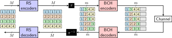
Figure 1: Example of an RS-BCH concatenation with $M=4$ RS codewords and $m=5$ BCH codewords. Each square represents one ($B$-bit) RS symbol and the number in each square represents the RS codeword index from which that symbol originates. Here, $K=4$, $N=5$, $k=4B$.

II System Model

Consider the concatenation of $M$ outer RS codes and $m$ inner BCH codes, as illustrated in Fig. 1. For simplicity, we assume throughout this paper that the outer codes are identical and the inner codes are identical. Each outer code is a (shortened) RS code $\mathcal{C}_{\text{RS}}(N,K,T)$ over $\mathbb{F}_{2^{B}}$ for some positive integer $B>1$. We will sometimes refer to RS symbols as ($B$-bit) bytes. Each inner code is a (shortened) BCH code $\mathcal{C}_{\text{BCH}}(n,k,t)$ over $\mathbb{F}_{2}$, where $k$ is an integer multiple of the byte size $B$.

We assume that all RS and BCH codewords are encoded systematically, i.e., the first $K$ bytes in an RS codeword are information symbols and the first $k$ bits in a BCH codeword are information bits. Furthermore, we assume that interleaving—i.e., the mapping of symbols—between outer and inner codes occurs in symbol-wise fashion: each RS symbol (represented as a string of $B$ bits) is interleaved into the information positions of a single BCH codeword. Such symbol-wise interleaving is commonly used in Ethernet standards and in optical transport networks [32, 24], and it simplifies our analysis; see also Remark 2 in Section IV.

Every symbol-wise interleaver induces an an $M\times m$ adjacency matrix $\mathbf{L}$, where $L_{i,j}$ (the entry in row $i$ and column $j$ of $\mathbf{L}$) is equal to the number of RS symbols interleaved from the $i$th outer code to the $j$th inner code. Such an adjacency matrix must satisfy the balance conditions

$$\sum_{j=1}^{m}{L}_{i,j}=N\quad\text{and}\quad B\sum_{i=1}^{M}{L}_{i,j}=k,$$ (1)

i.e., each outer code contributes $N$ symbols and each inner code receives $k$ bits.

Different symbol-wise interleavers may induce the same adjacency matrix $\mathbf{L}$. However, under bounded distance decoding of the constituent codes at the output of a binary symmetric channel (which is memoryless), each of them will have the same decoding performance. Thus we define the following standard interleaver that induces a given $\mathbf{L}$. For $i\in[M]^{*}$, let $\mathbf{C}_{i}\in\mathbb{F}_{2^{B}}^{N}$ denote a codeword of the $i$th RS code. We subdivide $\mathbf{C}_{i}$ into $m$ consecutive strips, writing

$$\mathbf{C}_{i}=\left(\mathbf{C}_{i,1},\mathbf{C}_{i,2},\ldots,\mathbf{C}_{i,m}\right),$$

where, for $j\in[m]^{*}$, the length of the $j$th strip is $L_{i,j}$ symbols. Then, for $j\in[m]^{*}$, the $j$th BCH codeword is given as

$$\mathbf{c}_{j}=\left(\mathbf{c}_{1,j},\mathbf{c}_{2,j},\ldots,\mathbf{c}_{M,j},\mathbf{c}^{\prime}_{j}\right),$$

where $\mathbf{c}_{i,j}$ is equal to the strip $\mathbf{C}_{i,j}$ represented as a string of $BL_{i,j}$ bits, and $\mathbf{c}^{\prime}_{j}$ denotes the $n-k$ parity bits of $\mathbf{c}_{j}$. The encoder architecture corresponding to this standard interleaver is summarized in Fig. 2.

Figure 2: Concatenated RS-BCH encoder architecture.

Example 1.

In Fig. 1, we have $M=4$ RS codewords $\mathbf{C}_{1},\ldots,\mathbf{C}_{4}$ over $\mathbb{F}_{2^{B}}$ that are interleaved into the information positions of the $m=5$ BCH codewords $\mathbf{c}_{1},\ldots,\mathbf{c}_{5}$. Each RS codeword has block length $N=5$ and each BCH codeword has dimension $k=4B$.

The RS codeword $\mathbf{C}_{1}$ contributes one symbol to each BCH codeword, thus $L_{1,1}=L_{1,2}=L_{1,3}=L_{1,4}=L_{1,5}=1$. The RS codeword $\mathbf{C}_{2}$ contributes no symbols to $\mathbf{c}_{1}$, but it does contribute one symbol to each of $\mathbf{c}_{2}$, $\mathbf{c}_{3}$, and $\mathbf{c}_{5}$, and two symbols to $\mathbf{c}_{4}$; thus $L_{2,1}=0$, $L_{2,2}=L_{2,3}=L_{2,5}=1$, and $L_{2,4}=2$. In similar fashion, we can determine the other entries of the adjacency matrix, arriving at

$$\mathbf{L}=\left[\begin{array}[]{ccccc}1&1&1&1&1\\ 0&1&1&2&1\\ 1&0&1&1&2\\ 2&2&1&0&0\end{array}\right].$$

Note that the sum of the entries in every row of $\mathbf{L}$ is $N=5$ and the sum of the entries in every column is $k/B=4$.

We are interested in estimating the decoded FER, i.e., the post-FEC FER. The main challenge is to translate error rates across the BCH-RS interface. In particular, BCH codes correct bit errors, while RS codes correct byte errors. The latter can therefore correct more than one bit for every corrected byte. The next two sections describe the relationship between bit errors and byte errors and the derivation of an expression of post-FEC FER assuming the binary symmetric channel.

III From Bits to Bytes

III-A Hamming Weight

Let $\mathbf{v}$ be a binary string of length $n$. The (usual) Hamming weight of $\mathbf{v}$, denoted $\operatorname{wt}(\mathbf{v})$, is the number of nonzero symbols that $\mathbf{v}$ contains. Now, let $B$ be any positive integer divisor of $n$. We define $w_{B}(\mathbf{v})$ as the Hamming weight of $\mathbf{v}$ when $\mathbf{v}$ is regarded as an element of $(\{0,1\}^{B})^{n/B}$, i.e., as a string of length $n/B$ over the alphabet $\{0,1\}^{B}$. The zero element of $\{0,1\}^{B}$ is the all-zero $B$-tuple $(0,\ldots,0)$, while all other elements of $\{0,1\}^{B}$ are nonzero and thus contribute to $w_{B}(\mathbf{v})$ when they occur in one of the $n/B$ positions of $\mathbf{v}$.

Example 2.

The string $\mathbf{v}=000111\in\{0,1\}^{6}$ has Hamming weight $w_{1}(\mathbf{v})=\operatorname{wt}(0,0,0,1,1,1)=3.$ When considered as a string over the quaternary ($B=2$) alphabet $\{00,01,10,11\}$, the same string has length $3$ and weight $w_{2}(\mathbf{v})=\operatorname{wt}(00,01,11)=2.$ When considered as a string over the octonary ($B=3$) alphabet $\{000,001,\ldots,111\}$, the string has length $2$ and weight $w_{3}(\mathbf{v})=\operatorname{wt}(000,111)=1.$

In the following, the elements of $\{0,1\}$ are referred to as bits, while the symbols of $\{0,1\}^{B}$ are referred to as ($B$-bit) bytes.

III-B Generating Functions

To keep track of the relationships between the different notions of Hamming weight, we will use generating functions. For any positive integer $n$, for any positive integer divisor $B$ of $n$, and for any set $\mathcal{S}\subseteq\{0,1\}^{n}$, let

$$W_{\mathcal{S}}(x,y)=\sum_{\mathbf{v}\in\mathcal{S}}x^{w_{1}(\mathbf{v})}y^{w_{B}(\mathbf{v})}.$$

In $W_{\mathcal{S}}(x,y)$, the indeterminate $x$ tracks bit-wise Hamming weight while the indeterminate $y$ tracks byte-wise Hamming weight. For $i,j\in\mathbb{N}$, the coefficient of the monomial $x^{i}y^{j}$ in $W_{\mathcal{S}}(x,y)$, denoted as $\operatorname{coeff}_{x^{i}y^{j}}(W_{\mathcal{S}})$, is equal to the number of vectors of $\mathcal{S}$ having bit-wise Hamming weight $i$ while simultaneously having byte-wise Hamming weight $j$.

As usual, since Hamming weight is additive over components, the key advantage of using generating functions is that the Cartesian product relation

$$W_{\mathcal{S}^{L}}(x,y)=W_{\mathcal{S}}^{L}(x,y)$$ (2)

holds, where $\mathcal{S}^{L}$ denotes the $L$-fold Cartesian product of the set $\mathcal{S}$ with itself.

Fix a byte size $B$, and let $W_{B,1}(x,y)=W_{\{0,1\}^{B}}(x,y)$ be the generating function corresponding to a single $B$-bit byte. We then have

$$W_{B,1}(x,y)=1+((1+x)^{B}-1)y=1+y\sum_{i=1}^{B}\binom{B}{i}x^{i},$$

which is explained as follows. The constant coefficient $\operatorname{coeff}_{x^{0}y^{0}}(W_{B,1})=1$, indicating that exactly one word (the all-zero word) simultaneously has bit-wise Hamming weight zero and byte-wise Hamming weight zero. For $i>0$, $\operatorname{coeff}_{x^{i}y}=\binom{B}{i}$, indicating that there are $\binom{B}{i}$ non-zero bytes having bitwise Hamming weight $i$ and byte-wise Hamming weight 1. For $j>1$, $\operatorname{coeff}_{x^{i}y^{j}}=0$, as there are no words with byte-wise Hamming weight greater than 1.

More generally, let $W_{B,L}(x,y)$ denote the generating function for $\{0,1\}^{BL}$, the collection of all binary strings of length $BL$, or equivalently, strips of length $L$ ($B$-bit) bytes. The Cartesian product relation (2) then gives

$$W_{B,L}(x,y)=W_{B,1}^{L}(x,y)=(1+((1+x)^{B}-1)y)^{L}.$$ (3)

If $L=0$, then the strip $\mathbf{v}$ is empty. For the empty string $\mathbf{v}$, we define $w_{1}(\mathbf{v})=w_{B}(\mathbf{v})=0$ and $W_{B,0}(x,y)=1$.

For our analysis of a concatenated RS-BCH code with $M$ outer RS codes, we now extend the idea of enumerating the Hamming weights of a single strip to enumerating the various Hamming weights of a string composed of $M$ strips of bytes, with each strip possibly having a different length. Let $\lambda=(L_{1},\ldots,L_{M})$ be an $M$-tuple of nonnegative strip-lengths $L_{1},\ldots,L_{M}$ and let $k=B(L_{1}+\cdots+L_{M})$. Let $\mathbf{v}=(\mathbf{v}_{1},\ldots,\mathbf{v}_{M},\mathbf{v}^{\prime})\in\{0,1\}^{n}$ be a binary string of length $n\geq k$, with strips $\mathbf{v}_{i}\in\{0,1\}^{BL_{i}}$ for $i\in[M]^{*}$, and $\mathbf{v}^{\prime}\in\{0,1\}^{n-k}$. We say that $\mathbf{v}$ is partitioned into strips according to $\lambda$. In our application, $\mathbf{v}$ is the $j$th BCH codeword, $\lambda$ is given by the $j$th column of the adjacency matrix $\mathbf{L}$, the $M$ strips $\mathbf{v}_{1},\ldots,\mathbf{v}_{M}$ correspond to the outer RS symbols interleaved to that codeword, and $\mathbf{v}^{\prime}$ corresponds to the parity bits of the BCH code (which are not passed to the outer codes).

For any subset $\mathcal{S}\subseteq\{0,1\}^{n}$ of binary strings partitioned according to $\lambda$, let

$$W_{\mathcal{S}}(x,y_{1},\ldots,y_{M})=\sum_{\mathbf{v}\in\mathcal{S}}x^{w_{1}(\mathbf{v})}y_{1}^{w_{B}(\mathbf{v}_{1})}y_{2}^{w_{B}(\mathbf{v}_{2})}\cdots y_{M}^{w_{B}(\mathbf{v}_{M})}$$

be a multivariate generating function. The indeterminate $x$ tracks the bit-wise Hamming weight of the elements of $\mathcal{S}$, while for $i\in[M]^{*}$, $y_{i}$ keeps track of the byte-wise Hamming weights of the strips $\mathbf{v}_{i}$ within the elements of $\mathcal{S}$.

Now, taking $\mathcal{S}=\{0,1\}^{n}$ (the set of all binary $n$-tuples), let

$$W_{B,n,\lambda}(x,y_{1},y_{2},\ldots,y_{M})=W_{\{0,1\}^{n}}(x,y_{1},\ldots,y_{M})$$

be the corresponding generating function. Similar to before, since Hamming weight is additive over components, we can represent $W_{B,n,\lambda}$ as

$$W_{B,n,\lambda} (x,y_{1},y_{2},\ldots,y_{M})$$

$$=W_{B,L_{1}}(x,y_{1})\cdot\cdots\cdot W_{B,L_{M}}(x,y_{M})\cdot(1+x)^{n-k}$$

$$=\left[\prod_{i=1}^{M}(1+((1+x)^{B}-1)y_{i})^{L_{i}}\right](1+x)^{n-k}.$$ (4)

The coefficient of $x^{\ell}y_{1}^{r_{1}}y_{2}^{r_{2}}\cdots y_{M}^{r_{M}}$ of $W_{B,n,\lambda}$, denoted by $\operatorname{coeff}_{x^{\ell}y_{1}^{r_{1}}y_{2}^{r_{2}}\cdots y_{M}^{r_{M}}}(W_{B,n,\lambda})$, represents the number of patterns in $\{0,1\}^{n}$ of bit-wise Hamming weight $\ell$, having byte-wise Hamming weights $r_{1},r_{2},\ldots,r_{M}$ in strips $1,2,\ldots,M$, respectively.

Example 3.

Consider $B=2$, $M=2$, $\lambda=(1,1)$ (thus $k=2(1+1)=4$) and $n=5$. We then have

$$W_{B,n,\lambda}(x,y_{1},y_{2})\\ =(1+((1+x)^{2}-1)y_{1})(1+((1+x)^{2}-1)y_{2})(1+x)\\ =1+x+2xy_{1}+2xy_{2}+3x^{2}y_{1}+3x^{2}y_{2}+4x^{2}y_{1}y_{2}\\ \quad+x^{3}y_{1}+x^{3}y_{2}+8x^{3}y_{1}y_{2}+5x^{4}y_{1}y_{2}+x^{5}y_{1}y_{2}.$$

Binary strings in $\{0,1\}^{5}$ having binary Hamming weight $\ell$, while having byte-wise Hamming weight $r_{1}$ and $r_{2}$ in $c_{1}$ and $c_{2}$, respectively, can be grouped as shown in Table I.

TABLE I: Length-5 Binary Strings with $B=2$, $M=2$, $\lambda=(1,1)$

$\ell$	$r_{1}$	$r_{2}$	# Strings	Term	Strings
$0$	$0$	$0$	$1$	$1$	$(00\,00\,0)$
$1$	$0$	$0$	$1$	$x$	$(00\,00\,1)$
$1$	$1$	$0$	$2$	$xy_{1}$	$(10\,00\,0)$, $(01\,00\,0)$
$1$	$0$	$1$	$2$	$xy_{2}$	$(00\,10\,0)$, $(00\,01\,0)$
$2$	$1$	$0$	$3$	$x^{2}y_{1}$	$(11\,00\,0)$, $(10\,00\,1)$, $(01\,00\,1)$
$2$	$0$	$1$	$3$	$x^{2}y_{2}$	$(00\,11\,0)$, $(00\,10\,1)$, $(00\,01\,1)$
$2$	$1$	$1$	$4$	$x^{2}y_{1}y_{2}$	$(10\,10\,0)$, $(10\,01\,0)$, $(01\,01\,0)$, $(01\,10\,0)$
$3$	$1$	$0$	$1$	$x^{3}y_{1}$	$(11\,00\,1)$
$3$	$0$	$1$	$1$	$x^{3}y_{2}$	$(00\,11\,1)$
$3$	$1$	$1$	$8$	$x^{3}y_{1}y_{2}$	$(11\,10\,0)$, $(11\,01\,0)$, $(10\,11\,0)$, $(01\,11\,0)$, $(10\,10\,1)$, $(10\,01\,1)$, $(01\,10\,1)$, $(01\,01\,1)$
$4$	$1$	$1$	$5$	$x^{4}y_{1}y_{2}$	$(11\,11\,0)$, $(11\,10\,1)$, $(11\,01\,1)$, $(10\,11\,1)$, $(01\,11\,1)$
$5$	$1$	$1$	$1$	$x^{5}y_{1}y_{2}$	$(11\,11\,1)$

IV Predicting the Frame Error Rate

IV-A Miscorrection-Free Analysis

Suppose now that binary strings of length $n$ are drawn at random according to any probability distribution satisfying the property that strings $\mathbf{v}$ with a fixed bit-level Hamming weight $w_{1}(\mathbf{v})$ all have the same probability of occurrence. We refer to any such distribution as being quasi-uniform by weight.

For example, if the individual bits within $\mathbf{v}$ are drawn independently according to a Bernoulli($p$) distribution (where $p$ denotes the probability of drawing “1”), then strings $\mathbf{v}$ with $w_{1}(\mathbf{v})=i$ all have the same probability of occurrence, namely $p^{i}(1-p)^{n-i}$.

We consider the decoder architecture summarized in Fig. 3. We begin by analyzing miscorrection-free decoders, i.e., hypothetical decoders that are able to correct error patterns of weight up to their decoding radius, while declaring a decoding failure when error patterns of higher weight are encountered. A miscorrection-free decoder never increases the weight of an error pattern by decoding to an incorrect codeword, which is an unrealistic assumption when the decoding radius is small. The influence of miscorrections is incorporated into the analysis in Section IV-B.

Suppose that all-zero codewords are transmitted. A miscorrection-free binary $t$-error correcting (BCH) decoder at the output of a binary symmetric channel would map all strings (representing error patterns) of bit-level Hamming weight $t$ or fewer to the all-zero string, while acting as an identity map on strings of Hamming weight greater than $t$. The output of this decoder would then also have a distribution that is quasi-uniform by weight.

More concretely, let $U_{j}$ denote the number of bit errors (i.e., the binary Hamming weight) in the received BCH$(n,k,t)$ codeword $\mathbf{c}_{j}=(\mathbf{c}_{1,j},\ldots\mathbf{c}_{M,j},\mathbf{c}_{j}^{\prime})$. The probability mass function of $U_{j}$ depends on the type of channel that is used. For example, for a binary symmetric channel with crossover probability $p$, we have

$$\Pr(U_{j}=\ell)=\binom{n}{\ell}p^{\ell}(1-p)^{n-\ell}\quad\text{for all}~{}\ell\in[n].$$ (5)

Let $\overline{U}_{j}$ be the number of bit errors of the BCH codeword $\overline{\mathbf{c}}_{j}=(\overline{\mathbf{c}}_{1,j},\ldots,\overline{\mathbf{c}}_{M,j},\overline{\mathbf{c}}_{j}^{\prime})$ remaining at the output of the $j$-th BCH decoder, i.e., after inner decoding. In the case of a miscorrection-free inner decoder, we have

$$\Pr(\overline{U}_{j}=\ell)=\begin{cases}\sum_{i=0}^{t}\Pr(U_{j}=i)&\ell=0,\\ 0&\ell=1,\ldots,t,\\ \Pr(U_{j}=\ell)&\ell=t+1,\ldots,n.\end{cases}$$ (6)

We can now compute the number of byte errors in strip $\overline{\mathbf{c}}_{i,j}$ for each $i\in[M]^{*},j\in[m]^{*}$. Let $\mathbf{V}_{j}=(V_{1,j},\ldots,V_{M,j})$, where $V_{i,j}$ is the number of byte errors in the strip $\overline{\mathbf{c}}_{i,j}$. Then for all $\ell\in[n]$ and $\mathbf{v}_{j}\in[L_{1,j}]\times\cdots\times[L_{M,j}]$,

$$\Pr(\mathbf{\mathbf{V}}_{j}=\mathbf{v}_{j})=\sum_{\ell=0}^{n}\Pr(\mathbf{\mathbf{V}}_{j}=\mathbf{v}_{j}\mid\overline{U}_{j}=\ell)\Pr(\overline{U}_{j}=\ell)\\ =\sum_{\ell=0}^{n}\frac{\operatorname{coeff}_{x^{\ell}y_{1}^{v_{1,j}}\cdots y_{M}^{v_{M,j}}}(W_{B,n,\lambda_{j}})}{\binom{n}{\ell}}\Pr(\overline{U}_{j}=\ell),$$

where $W_{B,n,\lambda_{j}}$ is as defined in (4) with $\lambda_{j}=(L_{1,j},\ldots,L_{M,j})$.

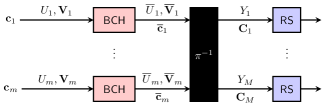
Figure 3: Concatenated RS-BCH decoder architecture.

Turning now to the perspective of the outer RS decoders, for any $i\in[M]^{*}$, let $Y_{i}$ denote the number of byte errors passed to the $i$th RS codeword $\mathbf{C}_{i}=(\mathbf{C}_{i,1},\ldots,\mathbf{C}_{i,m})$. Then $Y_{i}=V_{i,1}+\cdots+V_{i,m}$. Written as a vector random variable,

$$(Y_{1},\ldots,Y_{M}) =(V_{1,1},\ldots,V_{M,1})+\cdots+(V_{1,m},\ldots,V_{M,m})$$

$$=\mathbf{V}_{1}+\cdots+\mathbf{V}_{m}.$$ (7)

The $\mathbf{V}_{j}$’s are mutually independent, because they are obtained from independent BCH decoders. The joint distribution of $(Y_{1},\ldots,Y_{M})$ can therefore be obtained by convolving the distributions of the $\mathbf{V}_{j}$’s.

An RS decoder is unable to correct an error pattern containing more than $T$ bytes in error. A frame error (FE) occurs if one or more RS decoders are unable to correct their error patterns. The frame error rate is given by

$$\Pr(\text{FE})=\Pr\left((Y_{1}>T)\vee\cdots\vee(Y_{M}>T)\right).$$ (8)

Computing the exact frame error rate is difficult due to the correlation between the symbols in different RS codewords. However, we can bound the frame error rate via the union bound

$$\Pr(\text{FE})\leq\sum_{i=1}^{M}\Pr(Y_{i}>T).$$ (9)

Fig. 4 compares the computed FER values obtained from (9) against those computed via a Monte Carlo simulation assuming miscorrection-free decoders. We observe that the simulated data points agree closely with those computed using (9).

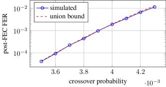
Figure 4: FER versus crossover probability for 8 $\times$ RS(544, 514, 15) outer code and 50 $\times$ BCH(940, 880, 6) inner code. We assume that both outer and inner decoders are miscorrection-free.

Remark 1.

While we have chosen to estimate the FER, our generating function approach is easily modified to estimate the bit error rate (BER) instead. See Appendix -A for details.

Remark 2.

In the crossover probability regime of most interest to optical communications, bit-error patterns typically result in one bit error per byte error. Thus, we would expect that performing bit-level interleaving rather than symbol-level interleaving (as analyzed here) would lead to similar post-FEC FER or BER.

Remark 3.

Generalization of this analysis to the situation where inner and outer codes have varying code parameters is straightforward, though cumbersome. Multiple generating functions would need to be introduced to track the error weights transferred from the various inner codes to the outer codes. The essential insight remains that the BCH decoders operate independently, leading to a sum of independent random variables as in (7), for the error weight seen by any particular RS decoder.

IV-B Effects of Miscorrection

In practice, algebraic decoders will not be miscorrection-free. A miscorrection, i.e., correction to a codeword not actually transmitted, can occur when the weight of the error pattern exceeds the decoding radius. For simplicity, this section will consider miscorrections in the inner BCH codes, but the result can be generalized to include miscorrections in the outer RS codes. We continue to assume that all-zero codewords are transmitted.

In general, any decoding procedure can be thought as a transformation of the error weight of the received word. More concretely, suppose that $U$ and $\overline{U}$ respectively denote the number of bit errors of the vector at the input and output of a BCH decoder with decoding radius $t$. Also, let $p_{u}=\Pr(U=u)$. In the case of a bounded-distance algebraic decoder, miscorrections may occur when $u$ is higher than the decoding radius. Thus, for $u\geq t+1$,

$$\Pr(\overline{U}=u)=f(p_{u-t},p_{u-t+1},\ldots,p_{u+t})$$

for some function $f$ which depends on the code.

Determining the weight distribution of the output of an algebraic decoder conditioned on the all-zero codeword being sent is, in general, a difficult problem. Error weights of $t$ or smaller are mapped to zero error weight (since the decoder can correct the errors) while, depending on the code, error weights larger than $t$ may result in an output error weight that depends on the particular input pattern. In case of a decoding failure the output error weight will be equal to the input error weight, while in the case of a miscorrection, the output error weight will match the weight of a nonzero codeword.

To estimate the output error weight from the input error weight, we will make the following assumptions.

1. When a miscorrection occurs, a word of error weight $w>t$ is miscorrected to a codeword of weight $w+t$.

2. Given that the received word has more than $t$ errors, the conditional miscorrection probability of a $t$-error correcting BCH code of length $n$ shortened from length $n_{\text{BCH}}$, is at most [33, 34]

   $$\frac{1}{t!}\left(\frac{n}{n_{\text{BCH}}}\right)^{t}.$$

   This assumption allows us to ignore the effects of miscorrections when $t$ is sufficiently large.

The first assumption is justified as follows. In the crossover probability regime of interest ($p<10^{-3}$), the error weight $w$ of the received word will only very rarely exceed $np+7\sqrt{np}$, i.e., 7 standard deviations above the mean, thus $w\ll n$. Let $A_{i}$ denote the number of codewords of weight $i$ in a $t$-error-correcting binary BCH code of length $n$. Clearly $A_{i}=0$ for all $i\in\{1,2,\ldots,2t\}$; and it is known [35] that $A_{i}\approx 2^{-(n-k)}\binom{n}{i}$ for $i\in\{2t+1,\ldots,n-2t-1\}$. Suppose that the all-zero codeword is sent and that the decoder miscorrects a word of weight $w>t$ to a codeword of weight $w^{\prime}\in\{w-t,w-t+1,\ldots,w+t\}$ at random. The probability that the codeword will have weight $w^{\prime}$ would then be

$$\frac{A_{w^{\prime}}}{A_{w-t}+\cdots+A_{w+t}}.$$

For $w\ll n$, we have $A_{w+t}\gg A_{w+t-1}\gg\cdots\gg A_{w-t}$, so $\Pr(w^{\prime}=w+t)\approx 1$. Thus, in the event of a miscorrection, it is very likely that a word of weight $w$ is miscorrected to a codeword of weight $w+t$ rather than to some other weight.

We now define a sequence of genie-aided decoders $D_{\ell}$, for $\ell=0,1,2,\ldots$, in which $D_{\ell}$ declares a decoding failure upon receipt of a word of error weight $t+1+\ell$ or greater, but otherwise attempts to decode. Thus $D_{0}$ is the miscorrection-free decoder, $D_{1}$ will suffer miscorrections due to attempting to decode words of error weight $t+1$, $D_{2}$ will suffer miscorrections due to attempting to decode words of error weight $t+1$ and $t+2$, etc.

We can estimate the performance of these decoders under the assumptions stated above. Table II gives the post-FEC BER for length-500 BCH codes with $t=1,2,3,4,5$ assuming a binary symmetric channel with crossover probability $p=1/n=2\cdot 10^{-3}$. Also included in the table are our estimated error rates for the genie-aided decoders $D_{0},D_{1},\ldots,D_{5}$.

TABLE II: Predicted Post-FEC BER for BCH Codes With and Without Miscorrection ($n=500,p=2\cdot 10^{-3}$)

	$t=1$	$t=2$	$t=3$	$t=4$	$t=5$
Actual	1.78e-3	6.75e-4	1.77e-4	3.79e-5	7.18e-6
$D_{0}$ Estimate	1.26e-3	5.27e-4	1.60e-4	3.75e-5	7.17e-6
$D_{1}$ Estimate	1.63e-3	6.44e-4	1.74e-4	3.84e-5	7.21e-6
$D_{2}$ Estimate	1.74e-3	6.73e-4	1.77e-4	3.86e-5
$D_{3}$ Estimate	1.77e-3	6.79e-4	1.77e-4
$D_{4}$ Estimate	1.78e-3	6.79e-4
$D_{5}$ Estimate	1.78e-3

We see that for $t=1$ BCH codes (i.e., Hamming codes), the post-FEC BER agrees closely with the simulation when we consider the effects of miscorrection up to words of error weight $t+4=5$ (i.e., under decoding with $D_{4}$). For $t=2$ and $t=3$ BCH codes, the predicted BERs under $D_{2}$ already closely match the simulation. When $t\geq 4$, predicted BERs under $D_{0}$ (the miscorrection-free decoder) closely agree with the simulated value.

We conclude that, in the crossover probability regime of interest, adjusting error-rate estimates to take miscorrections into account is important only for $t\leq 3$. For $t=1$, $2$, and $3$, we will consider miscorrections only for received words of error weight up to $5$ (i.e., genie-aided decoder $D_{4}$ for $t=1$, $D_{3}$ for $t=2$, and $D_{2}$ for $t=3$). We will assume that error weights greater than 5 lead to a decoding failure.

Remark 4.

In the case of extended Hamming codes, miscorrections occur only when the received error weight is odd. Using a similar argument as above, in the event of a miscorrection, a word of odd weight $w>2$ is assumed to be miscorrected to a codeword of weight $w+1$.

Fig. 5 shows post-FEC FER curves comparing Monte Carlo simulation with predicted FER using our analysis (5)–(9) with and without miscorrections taken into account. The plot for the predicted FER with miscorrection closely agrees with the plot obtained from the simulation.

Note that since we are interested in the post-FEC FER, not the BER, we do not need to take the miscorrection rate of the outer RS codes into account. Any RS word receiving more than $T$ byte errors is already sufficient to trigger a frame error.

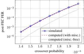
Figure 5: FER versus crossover probability for 8 $\times$ RS(544, 514, 15) outer code and 64 $\times$ BCH(700, 680, 2) inner code with and without miscorrection taken into account. We take miscorrection into account only for received BCH words of error weights 3, 4, and 5.

V Performance-Complexity-Latency Trade-offs

V-A Metrics

In this subsection, we will define and describe appropriate metrics for performance, complexity, and latency of concatenated RS-BCH codes.

V-A1 Performance

We define the performance of a code as the gap to the Shannon limit (in dB) for a binary symmetric channel at $10^{-13}$ post-FEC FER. The binary symmetric channel is assumed to arise as additive white Gaussian noise channel with antipodal input under hard-decision detection, so a gap in dB measures a noise-power ratio. Let $R$ and $p^{*}$ denote the code rate and the channel crossover probability such that the post-FEC FER is $10^{-13}$, respectively. The gap to the Shannon limit is then obtained as

$$\text{Gap (dB)}=20\log_{10}\left(\frac{\operatorname{erfc}^{-1}(2p^{*})}{\operatorname{erfc}^{-1}\left(2\mathcal{H}^{-1}(1-R)\right)}\right),$$

where $\operatorname{erfc}^{-1}$ denotes the inverse complementary error function, and $\mathcal{H}^{-1}$ denotes the inverse binary entropy function returning values in $[0,\frac{1}{2}]$.

Of course, other performance metrics, such as net coding gain (used in [21]) might be considered.

V-A2 Complexity

We define the complexity to be the total number of elementary operations performed by the inner and outer decoders in the worst case, normalized by the number of information bits of the overall concatenated code. As shown in Appendix -B, using a discrete logarithm-domain representation of finite field elements, all decoding operations are implemented in terms of integer addition and subtraction and table lookup.

There are five main RS/BCH decoding procedures to consider:

1. syndrome computation (SC),

2. key equation solver (KE),

3. polynomial root-finding (RF),

4. error evaluation (EE) (for RS decoder only), and

5. bit correction (BC).

A detailed analysis of the complexity of each decoding step is given in Appendices -C–-E and the results are summarized in Table III. For values of $t$ and $T$ smaller than 5, simplified procedures for the KE and RF steps are assumed, as explained in Appendices -D and  -E. For values of $t$ and $T$ greater than 4, general-purpose algorithms (Berlekamp-Massey and Chien search) are assumed.

The complexity of an RS decoder is the sum of the complexities of the SC, KE, RF, EE, and BC procedures, denoted as $\kappa_{\text{RS}}$. The complexity of a BCH decoder is the sum of the complexities of the SC, KE, RF, and BC procedures, denoted as $\kappa_{\text{BCH}}$. Thus, since the concatenated code has $M$ RS decoders and $m$ BCH decoders with $MKB$ information bits, the number of operations per decoded information bit is given as

$$\dfrac{M\kappa_{\text{RS}}+m\kappa_{\text{BCH}}}{MKB}.$$

TABLE III: Number of Operations for RS and BCH Decoding, Worst Case

Operation	# Ops. (RS)	# Ops. (BCH)
SC	$6K(N-K)$	$nt$
KE ($T=1$)	$9$	$0$
KE ($T=2$)	$54$	$11$
KE ($T=3$)	$159$	$23$
KE ($T=4$)	$336$	$64$
KE ($T\geq 5$)	$2T(24T+8)$	$2t(24t+8)$
RF ($T=1$)	$0$	$0$
RF ($T=2$)	$10$	$10$
RF ($T=3$)	$37$	$37$
RF ($T=4$)	$98$	$98$
RF ($T\geq 5$)	$6NT$	$6nt$
EE	$T\left(6(2T+\lceil T/2\rceil)-1\right)$	—
BC	$2T$	$t$

Note that making different architectural or algorithmic assumptions may give different formulas for the complexity measure.

V-A3 Latency

Latency is typically defined as the length of time between when a particular information bit arrives at the input of the encoder and when its estimate leaves the output of the decoder. When high-rate systematic codes are used, bits are transmitted essentially as soon as they arrive. They undergo modulation, propagation over the channel, channel equalization and receiver filtering, etc., and then are accumulated in a receiver buffer. Decoding commences once the receiver buffer is full. Assuming a single decoder, the decoding time is normally set equal to the time it takes to fill the receiver buffer, since decoding more slowly than this is not possible (otherwise codewords would accumulate faster than they can be decoded) and decoding more quickly than this is not necessary (otherwise the decoder would undergo idle periods). Since signal-processing delays are usually negligible compared with propagation and buffer-fill delays, in most applications, the latency is dominated by the sum of the propagation delay and double the time it takes to fill the receiver buffer. Since latter is proportional to the block length of the concatenated code, we take the block length $mn$ as our latency metric.

V-B Code Search

We are interested in determining combinations of inner and outer code parameters leading to the best possible tradeoffs between performance, complexity, and latency. We first fix the target rate and an upper bound on latency of our system. We then sweep through the following outer RS and inner BCH code parameters:

• outer code parameters: $5\leq B\leq 10$, $N\leq 2^{B}-1$, $0\leq T\leq 20$, $K=N-2T$;

• inner code parameters: $7\leq b\leq 14$, $n\leq 2^{b}-1$, $0\leq t\leq 15$, $k=n-bt$, $B\mid k$. When $t=1$, we consider using both Hamming codes and extended Hamming codes, and in the latter case, $t=1\text{x}$ and $k=n-b-1$. The case $t=0$ corresponds to a system with $M$ outer RS codes and a trivial (rate one) inner code. Similarly, the case $T=0$ corresponds to a system with $m$ inner BCH codes and a trivial (rate one) outer code.

We adjust the number of BCH codewords $m$ such that the latency $mn$ is not greater than the latency bound. We then compute $M=\left\lfloor\frac{mk}{NB}\right\rfloor$. In the case of $MNB<mk$, we assume that the information positions of the first $m-1$ BCH codewords are completely filled in with the bits from the RS codewords. The remaining $mk-MNB$ information bits in the last BCH codeword are zero-padded. We also make sure that the code rate $R=MKB/mn$ is approximately the same as the target rate. In our code search, we have $|R-\text{target rate}|\leq 0.05$, i.e, we achieve a rate within $5\%$ of the target rate.

Finally, the interleaving scheme is chosen such that in the adjacency matrix $\mathbf{L}$, we have $L_{ij}\approx N/m$ (or $\approx k/BM$) for all $i\in[M]^{*}$, $j\in[m]^{*}$. This is achieved by picking the entries of $\mathbf{L}$ in the set $\left\{\left\lfloor N/m\right\rfloor,\left\lceil N/m\right\rceil\right\}$ such that $\mathbf{L}$ satisfies (1). This ensures that each RS codeword contributes an (almost) equal number of bits to each BCH codeword.

We note that in the case of a sufficiently high BCH decoding radius $t$ and for a sufficiently low code rate, the number of parity bits in a BCH codeword of length $2^{b}-1$ can actually be fewer than $bt$ (or equivalently, the code dimension can be higher than $n-bt$) [36]. In this code search, we search for codes with rates $0.85$ and $239/255\approx 0.937$, and for BCH codes with such rates (or higher), we have verified that $k=n-bt$ is indeed the highest possible BCH code dimension for a given $n$, $b$, and $t$.

We emphasize that no Monte Carlo simulations are needed to evaluate the various codes being considered. Given the code parameters and channel crossover probability, the FER is estimated using (5)–(9). We then determine the appropriate crossover probability such that the post-FEC FER is $10^{-13}$ and compute the gap to the Shannon limit.

The Pareto optimal code parameters from the code search parameters described above with rate targets of $0.85$ and $239/255\approx 0.937$ are shown in Figs. 6 and 7. The parameters of a subset of the codes on the Pareto frontier are shown in Tables IV and V; see Appendix -F for a complete listing.

It is also interesting to note that for most of the code parameters on the Pareto frontier, the codes comprise weak ($t\leq 4$) inner codes combined with much stronger RS outer codes. At very low complexities, we find that many $T=0$ codes (rate-1 outer codes, i.e., error protection only from the BCH codes) are Pareto efficient.

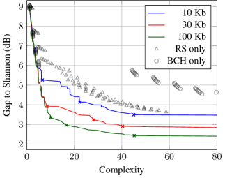
Figure 6: Performance-complexity-latency trade-offs for target rate $\approx 0.85$. Each curve shows Pareto-efficient operating points corresponding to a fixed upper bound on code latency as indicated. For a latency bound of 10Kb, approximately 10,000 codes were evaluated, among which 53 are Pareto-efficient. For a latency bound of 30Kb, approximately 450,000 codes were evaluated, among which 77 are Pareto-efficient. For a latency bound of 100Kb, approximately $4\times 10^{6}$ codes were evaluated, among which 162 are Pareto-efficient. The performance and complexity of RS codes and BCH codes of rate $0.85$ and latency at most 10Kb are also included. The points marked with “$\times$” correspond to the Pareto-efficient code parameters listed in Table IV.

TABLE IV: Some Pareto-Efficient Code Parameters, Rate $\approx 0.85$

$M$	$N$	$B$	$T$	$m$	$n$	$b$	$t$	Latency	Complexity	Gap (dB)
19	56	8	3	56	161	8	1x	9016	6.6	5.26
3	274	10	10	92	98	7	1x	9016	22.2	4.14
2	427	10	20	61	149	8	1x	9089	45.0	3.50
27	120	8	3	130	224	8	3	29120	8.6	3.92
6	420	10	12	115	244	8	3	28060	28.0	3.23
3	860	10	18	89	326	9	4	29014	40.3	2.91
27	314	10	4	340	286	9	4	97240	10.0	3.35
29	300	10	6	300	326	9	4	97800	16.7	2.97
11	747	10	20	249	366	9	4	91134	45.2	2.43

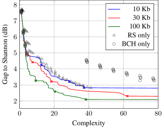
Figure 7: Performance-complexity-latency trade-offs for target rate $239/255\approx 0.937$. Each curve shows Pareto-efficient operating points corresponding to a fixed upper bound on code latency as indicated. For a latency bound of 10Kb, approximately 8,000 codes were evaluated, among which 64 are Pareto-efficient. For a latency bound of 30Kb, approximately 370,000 codes were evaluated, among which 109 are Pareto-efficient. For a latency bound of 100Kb, approximately $5\times 10^{6}$ codes were evaluated, among which 114 are Pareto-efficient. The performance and complexity of RS codes and BCH codes of rate $0.937$ and latency at most 10Kb are also included. The points marked with “$\times$” correspond to the Pareto-efficient code parameters listed in Table V.

TABLE V: Some Pareto-Efficient Code Parameters, Rate $\approx 0.937$

$M$	$N$	$B$	$T$	$m$	$n$	$b$	$t$	Latency	Complexity	Gap (dB)
2	391	10	6	17	472	11	1x	8024	12.6	4.23
1	445	10	14	—	—	—	—	4450	28.8	3.20
1	692	10	18	1	6933	13	1	6933	37.2	2.82
16	215	8	4	35	806	13	1x	28210	7.5	4.42
4	606	10	9	61	413	12	1x	25193	18.3	3.21
3	960	10	20	67	440	10	1x	29480	62.2	2.31
20	467	10	4	117	840	10	4	98280	9.3	3.26
13	646	10	9	86	1016	12	3	87376	20.4	2.59
9	952	10	18	68	1296	12	3	88128	38.3	2.10

VI Conclusion

In this paper, we have provided a formula to predict the frame error rate of the concatenated RS-BCH codes. We have determined the parameters of codes that are Pareto optimal with respect to particular measures of performance, complexity, and latency. The complexity measure simply counts the elementary operations (integer addition and subtraction and table lookups) required for decoding. Future work may include extending the complexity measure to reflect hardware implementation or energy consumption. Furthermore, it would be interesting to extend the FER analysis to a pseudo-product-code-like structure, where there is iterative decoding between the inner and outer codes.

VII Acknowledgment

The authors would like to thank the anonymous reviewers for their valuable comments and suggestions.

-A Predicting the Post-FEC Bit Error Rate (BER)

Suppose that the BCH and RS decoders are miscorrection-free. Recall from Sec. IV that $Y_{i}$ denotes the number of byte ($B$-bit symbol) errors at the input of the $i$th RS decoder. Let $\overline{Y}_{i}$ denote the number of byte errors at the output of the $i$th RS decoder. Then,

$$\Pr(\overline{Y}_{i}=0)=\sum_{y=0}^{T}\Pr(Y_{i}=y)$$

and

$$\Pr(\overline{Y}_{i}=y)=\Pr(Y_{i}=y)~{}\text{for all}~{}y=T+1,\ldots,N.$$

Thus, at the output of the $i$th RS decoder, we expect to see

$$E(\overline{Y}_{i})=\sum_{y=T+1}^{N}yP(\overline{Y}_{i}=y)$$ (10)

byte errors.

We will now estimate the number of bit errors in the event of a byte error. Let $Z$ denote the number of bit errors in a byte. For a binary symmetric channel with crossover probability $p$, we have

$$\Pr(Z=z)=\binom{B}{z}p^{z}(1-p)^{B-z}\quad\text{for all}~{}z\in[B].$$ (11)

Thus, in the event of a byte error, we expect to see

$$E(Z\mid Z>0)=\sum_{z=1}^{B}z\frac{P(Z=z)}{P(Z>0)}$$ (12)

bit errors. Hence, the post-FEC BER is approximately

$$\frac{(E(\overline{Y}_{1})+\cdots+E(\overline{Y}_{M}))E(Z\mid Z>0)}{MNB}.$$ (13)

Fig. 8 shows post-FEC BER curves comparing Monte Carlo simulation with predicted BER using our analysis (10)–(13). Similar to those in Figs. 4 and 5, we observe that the computed BERs agree closely with those computed (13).

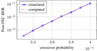
Figure 8: BER versus crossover probability for $8\times~{}\text{RS}(544,514,15)$ outer code and $68\times~{}\text{BCH}(690,640,5)$ BCH code. We assume that both outer and inner decoders are miscorrection-free.

-B Finite Field Arithmetic

In this appendix we show that, by using a discrete logarithm representation, finite field operations can be implemented using integer addition and subtraction and table lookups, and we derive the number of elementary operations needed.

Let $q=2^{b}$, and let $\alpha$ be a primitive element of $\mathbb{F}_{q}$. Every nonzero element $x\in\mathbb{F}_{q}$ is of the form $x=\alpha^{i}$, where $i\in[q-2]$. The exponent $i$ is the discrete logarithm of $x$ to the base $\alpha$, and we write $\log(x)=i$. For reasons that will become clear, we define $\log(0)=2q-3$.

-B1 Multiplication

Let $x,y\in\mathbb{F}_{q}$ with $\log(x)=i$ and $\log(y)=j$ for $i,j\in[q-2]\cup\{2q-3\}$. Then

$$\log(xy)=M(i+j),$$

where

$$M(\ell)=\begin{cases}\ell&\text{if}~{}0\leq\ell\leq q-2,\\ \ell-q+1&\text{if}~{}q-1\leq\ell\leq 2q-4,\\ 2q-3&\text{if}~{}2q-3\leq\ell\leq 4q-6.\end{cases}$$

We assume that the values of $M(\ell)$ are stored in a table with $4q-5$ entries. Thus, multiplying two elements in $\mathbb{F}_{q}$ comprises two elementary operations: one integer addition and one table lookup. We note that multiplication by zero could be handled conditionally; however, this table lookup approach avoids testing whether $x$ or $y$ is zero, resulting in fewer operations. Since $(q-2)+(q-2)=2q-4$, setting $\log(0)=2q-3$ (outside the range of the sum of logarithms of nonzero elements) minimizes the size of the $M$ table.

-B2 Addition

Let $x,y\in\mathbb{F}_{q}$ with $\log(x)=i$ and $\log(y)=j$ for $i,j\in[q-2]\cup\{2q-3\}$. If $i,j\in[q-2]$, then

$$\log(x+y) =\log\left(\alpha^{i}+\alpha^{j}\right)$$

$$=\log\left(\alpha^{i}\left(1+\alpha^{j-i}\right)\right)$$

$$=M\left(i+\log\left(1+\alpha^{j-i}\right)\right)$$

$$=M(i+Z(j-i)),$$ (14)

where

$$Z(\ell)=\begin{cases}\ell&\text{if}~{}-2q+3\leq\ell\leq-q+1,\\ \log(1+\alpha^{\ell})&\text{if}~{}-q+2\leq\ell\leq q-2,\\ 0&\text{if}~{}q-1\leq\ell\leq 2q-3.\end{cases}$$

We assume that the values of $Z(\ell)$, the Zech logarithm [37] extended to include $\log(0)$, are stored in a table with $4q-5$ entries, designed so that (14) holds even when one or both of $i$ and $j$ is $2q-3$. As with multiplication, this avoids testing whether one or both of the operands is the zero element. Thus, adding two elements in $\mathbb{F}_{q}$ comprises four elementary operations: one integer addition, one integer subtraction, and two table lookups.

-B3 Division

Let $x,y\in\mathbb{F}_{q}$ with $\log(x)=i$ and $\log(y)=j$ for $i\in[q-2]\cup\{2q-3\}$ and $j\in[q-2]$. Then,

$$\log(x/y) =M\left(\log(x)+\log(y^{-1})\right)$$

$$=M\left(i+I(j)\right),$$

where $I(j)=-j\bmod(q-1)$. We assume that the values of $I(j)$ are stored in a table with $q-1$ entries. The table lookup avoids performing a $\bmod(q-1)$ operation. Thus, dividing $x$ by (a nonzero) $y$ comprises three elementary operations: one integer addition and two table lookups.

-B4 Converting Between Polynomial and Discrete Logarithm Representations

Let $\alpha$ be a primitive element of $\mathbb{F}_{2^{m}}$. A polynomial representation of an element of $x\in\mathbb{F}_{2^{m}}$ is an expression of the form $x=x_{0}+x_{1}\alpha+\cdots+x_{m-1}\alpha^{m-1}$, where usually the polynomial coefficients are gathered into the $m$-tuple $(x_{0},\ldots,x_{m-1})\in\mathbb{F}_{2}^{m}$. We assume that there exist lookup tables that can be used to convert between polynomial and discrete logarithm representations of finite field elements.

-C RS/BCH Decoder Complexity

-C1 Syndrome Computation (SC)

We suppose that the parity-check matrix for the RS code is given in systematic form $H=[-P^{T}\mid I]$, where $P$ is a $K\times(N-K)$ matrix and $I$ is an $(N-K)\times(N-K)$ identity matrix. Computation of the syndrome corresponding to an $N$-byte vector then requires $(N-K)$ inner-product operations of length $K$ vectors, which requires $K(N-K)$ multiplications and $(K-1)(N-K)$ additions, and additional length $(N-K)$ vector addition, for a total of $K(N-K)$ multiplications, and $K(N-K)$ additions. This brings the number of elementary operations for SC to $4K(N-K)+2K(N-K)=6K(N-K)$.

The SC complexity for BCH codes, on the other hand, is composed of the XORs of columns of the parity-check matrix according to the zero/one pattern in the received word. We assume that each parity-check matrix column comprises $t$ $b$-bit symbols over $\mathbb{F}_{2^{b}}$ in their polynomial representation. Assuming that a symbol-wise XOR takes one operation, at most $(n-1)t$ operations are needed in total to compute the polynomial representation of the syndrome. We then convert from polynomial representation to the discrete logarithm representation, which takes another $t$ operations. In total, therefore, the number of elementary operations required for BCH syndrome computation is $nt$.

-C2 Key Equation Solver (KE)

There are two cases to consider to obtain the error-locator polynomial and, in the case of RS decoding, error-evaluator polynomial.

Case $T$ (or $t$) $=1,2,3,4$: If the error correcting radius of the RS decoder is small, the process of obtaining the coefficients of the error-locator polynomial can be simplified by using Peterson’s algorithm. Suppose that the RS syndromes obtained from SC are $(S_{1},S_{2},\ldots,S_{2T})$. The coefficients of the error-locator polynomial

$$\Lambda(x)=1+\Lambda_{1}x+\cdots+\Lambda_{\nu}x^{\nu}$$

for some $\nu\in[T]$ is obtained by solving a system of linear equations

$$S_{j}=\sum_{i=1}^{\nu}\Lambda_{i}S_{j-i}\quad\text{for all}~{}j\in[\nu]^{*}.$$

The worst-case complexity of the algorithm is attained when $\Lambda(x)$ has degree $T$, i.e., $\nu=T$. We use Gaussian elimination to solve for $\Lambda_{1},\ldots,\Lambda_{T}$. The number of operations needed is:

• $T=1$: 1 division,

• $T=2$: 3 additions, 3 multiplications, and 2 divisions,

• $T=3$: 12 additions, 15 multiplications, and 3 divisions,

• $T=4$: 30 additions, 36 multiplications, and 4 divisions.

In order to obtain the error-evaluator polynomial $\Omega(x)$ for RS decoders for $T=1,2,3,4$, we have

$$\Omega(x)= \Omega_{0}+\Omega_{1}x+\cdots+\Omega_{2T-1}x^{2T-1}$$

$$\equiv \Lambda(x)S(x)\bmod x^{2T},$$

where $S(x)=S_{1}+S_{2}x+\cdots+S_{2t}x^{2t-1}$. The modulo operation above denotes that terms of degree $2T$ and higher are discarded. Thus, assuming the worst-case complexity that $\deg\Lambda(x)=T$, we have $\Omega_{0}=S_{0}$ and

$$\Omega_{j}=S_{j}+\sum_{i=1}^{\min\{j,T\}}\Lambda_{i}S_{j-i}~{}\quad\text{for all}~{}j\in[2T-1]^{*},$$

which takes at most $\frac{1}{2}T(3T-1)$ additions and $\frac{1}{2}T(3T-1)$ multiplications. Thus, the complexity for computing the coefficients of $\Omega(x)$ is:

• $T=1$: 1 addition and 1 multiplication,

• $T=2$: 5 additions and 5 multiplications,

• $T=3$: 12 additions and 12 multiplications,

• $T=4$: 22 additions and 22 multiplications.

The total complexity of KE for an RS decoder with $T=1,2,3,4$ is therefore:

• $T=1$: $4+2+3=9$,

• $T=2$: $8\cdot 4+8\cdot 2+2\cdot 3=54$,

• $T=3$: $24\cdot 4+27\cdot 2+3\cdot 3=159$,

• $T=4$: $52\cdot 4+58\cdot 2+4\cdot 3=336$.

For BCH decoders, the algorithm can be simplified to even fewer operations, as described in Appendix -D.

Case $T$ (or $t$) $\geq 5$: We consider the Berlekamp-Massey algorithm to obtain the error-locator and error-evaluator polynomials. We assume the reformulated inversionless Berlekamp–Massey algorithm (RiBM) [38] with $2T(3T+1)$ additions and $2T(6T+2)$ multiplications. Using the same algorithm for BCH, KE takes $2t(3t+1)$ additions and $2t(6t+2)$ multiplications.

-C3 Polynomial Root-Finding (RF)

There are two cases to consider to determine the roots of the error-locator polynomial $\Lambda(x)$.

Case $T$ (or $t$) $=1,2,3,4$: For small $T$ or $t$, the roots of $\Lambda(x)$ can be determined by using lookup-table-based root-finding algorithms described in Appendix -E.

Case $T$ (or $t$) $\geq 5$: We perform a brute-force Chien search of the roots of $\Lambda(x)$. In the worst case scenario, $\Lambda(x)$ has to be evaluated $N$ times. Evaluating $\Lambda(x)$ with degree $T$, using Horner’s method, takes $T$ additions and $T$ multiplications, and so in total, the worst-case complexity for RF is $NT(4+2)$. Similarly, the worst-case complexity of RF for BCH is $nt(4+2)$.

-C4 Error Evaluation (EE)

The next part of RS decoding is to compute the error magnitude using Forney’s algorithm [39]. The worst-case complexity of EE is when the error-locator polynomial $\Lambda(x)$ has $T$ distinct roots, i.e., $\deg\Lambda(x)=T$.

Denote $\Lambda^{\prime}(x)=\Lambda_{1}+2\Lambda_{2}x+\cdots+\nu\Lambda_{T-1}x^{T-1}$ to be the formal derivative of $\Lambda(x)$. Since the code operates over a field of characteristic two, there are no odd-powered terms in $\Lambda^{\prime}(x)$, leaving $\Lambda^{\prime}(x)$ with up to $\lceil T/2\rceil$ nonzero even-powered terms. Thus, at every step of Horner’s method of polynomial evaluation, one can use $x^{2}$ instead of $x$ to reduce the number of additions and multiplications by a factor of two.

Suppose that $X_{i_{1}}^{-1},\ldots,X_{i_{T}}^{-1}$ are the roots of $\Lambda(x)$ obtained in the RF step above. Then, the error magnitude at position $i_{j}$ ($j=1,\ldots,T$) is

$$E_{j}=-\frac{\Omega(X_{i_{j}}^{-1})}{\Lambda^{\prime}(X_{i_{j}}^{-1})}.$$

The complexity therefore comprises two polynomial evaluations via Horner’s method plus one finite field division.

Evaluating $\Omega(X_{i_{j}}^{-1})$ takes $2T-1$ finite field additions and $2T-1$ multiplications. It takes one multiplication to compute $(X_{i_{j}}^{-1})^{2}$, and evaluating $\Lambda^{\prime}(X_{i_{j}}^{-1})$ takes $\lceil T/2\rceil$ additions and $\lceil T/2\rceil$ multiplications. Finally, we divide $\Omega(X_{i_{j}}^{-1})$ by $\Lambda^{\prime}(X_{i_{j}}^{-1})$. The total complexity of EE is therefore $T\left((2T+\lceil T/2\rceil-1)(4+2)+2+3\right)$.

-C5 Bit Correction (BC)

For a given RS word, there are up to $T$ bytes to be corrected. Assuming that there are $T$ byte errors that are to be corrected, the $T$ error magnitudes are first converted to the polynomial representation, which takes $T$ operations. Then, the bytes in the $T$ locations of the received word prescribed by the RF are XOR-ed by the error magnitude. Thus, it takes $2T$ operations.

On the other hand, there is no error evaluation needed for BCH decoding, and therefore the number of operations for BC is at most $t$.

-D Worst-Case Complexity of Simplified Peterson’s Algorithm for $t=1,2,3,4$ BCH Decoders

This section describes the complexity of obtaining the coefficients of the error locator polynomials using Peterson’s algorithm for $t=2,3,4$ binary BCH decoders with $n=2^{b}-1$ [40]. Throughout this section, assume that the syndromes for $t=1$, $2$, $3$, and $4$ BCH words have form $(S_{1})$, $(S_{1},S_{3})$, $(S_{1},S_{3},S_{5})$, and $(S_{1},S_{3},S_{5},S_{7})$, respectively, where $S_{1},S_{3},S_{5},S_{7}\in\mathbb{F}_{2^{b}}$. Also, for all positive integers $q$, let $D_{q}=S_{q}+S_{1}^{q}$. We also assume that division by zero never happens in the algorithm below.

-D1 $t=1$

The error-locator polynomial is

$$\Lambda(x)=1+S_{1}x.$$

The coefficient of $x$ can be obtained directly from the syndromes. This operation has zero complexity.

-D2 $t=2$

The error-locator polynomial is

$$\Lambda(x)=1+S_{1}x+\frac{D_{3}}{S_{1}}x^{2}.$$

One addition and two multiplications are required to obtain $D_{3}=S_{1}^{3}+S_{3}=S_{1}\cdot S_{1}\cdot S_{1}+S_{3}$. In order to obtain the coefficient of $x^{2}$, we perform one division. In total, we have one addition, two multiplications, and one inversion. The complexity is therefore $4+2\cdot 2+3=11$

-D3 $t=3$

The error-locator polynomial is

$$\Lambda(x)=1+\Lambda_{1}x+\Lambda_{2}x^{2}+\Lambda_{3}x^{3},$$

where

$$\Lambda_{1}=S_{1},~{}\Lambda_{2}=\frac{S_{1}^{2}S_{3}+S_{5}}{D_{3}},~{}\Lambda_{3}=D_{3}+S_{1}\Lambda_{2}.$$

We first compute and store the values of $S_{1}^{2}$ and $S_{1}^{3}$, each of which requires one multiplication. Then, computing $D_{3}$ takes one addition. Using the value of $S_{1}^{2}$ and $D_{3}$ obtained in the previous step, computing $\Lambda_{2}$ takes one addition, one multiplication, and one division. Finally, computing $\Lambda_{3}$ takes one addition and one multiplication. In total, we have three additions, four multiplications, and one division. The complexity is therefore $3\cdot 4+4\cdot 2+3=23$

-D4 $t=4$

The error-locator polynomial is

$$\Lambda(x)=1+\Lambda_{1}x+\Lambda_{2}x^{2}+\Lambda_{3}x^{3}+\Lambda_{4}x^{4},$$

where

$$\Lambda_{1}=S_{1},\quad\Lambda_{2}=\frac{S_{1}D_{7}+S_{3}D_{5}}{S_{3}D_{3}+S_{1}D_{5}},$$

$$\Lambda_{3}=D_{3}+S_{1}\Lambda_{2},\quad\Lambda_{4}=\frac{S_{5}+S_{1}^{2}S_{3}+D_{3}\Lambda_{2}}{S_{1}}.$$

We will compute and store a few intermediate terms listed in Table VI.

TABLE VI: Number of Operations of the Intermediate Terms for Computing the Coefficients of $\Lambda(x)$

Term	# Additions	# Multiplications
$S_{1}^{2}$	$0$	$1$
$S_{1}^{4}=S_{1}^{2}\cdot S_{1}^{2}$	$0$	$1$
$S_{1}^{6}=S_{1}^{4}\cdot S_{1}^{2}$	$0$	$1$
$D_{3}=S_{1}^{2}\cdot S_{1}+S_{3}$	$1$	$1$
$D_{5}=S_{1}^{4}\cdot S_{1}+S_{5}$	$1$	$1$
$D_{7}=S_{1}^{6}\cdot S_{1}+S_{5}$	$1$	$1$

The complexity to compute $\Lambda_{2},\Lambda_{3},\Lambda_{4}$ is listed below:

• $\Lambda_{2}$: 2 additions, 4 multiplications, and 1 division,

• $\Lambda_{3}$: 1 addition and 1 multiplication,

• $\Lambda_{4}$: 2 additions, 2 multiplications, and 1 division.

In total, we have 8 additions, 13 multiplications, and 2 divisions. The complexity is therefore $8\cdot 4+13\cdot 2+2\cdot 3=64$

-E Worst-Case Complexity of Root-Finding Algorithms for Polynomials of Degree $\leq 4$ over $\mathbb{F}_{2^{b}}$

The root-finding algorithms for degree-1, 2, and 3 polynomials are based on [41]. The root-finding algorithm for degree-4 polynomials is based on [42]. In these algorithms, aside from the lookup tables specified in Appendix -B, we also store lookup tables of:

• roots of $x^{2}+x+c=0$ for all $c\in\mathbb{F}_{2^{b}}$ (DP2),

• roots of $x^{3}+x+c=0$ for all $c\in\mathbb{F}_{2^{b}}$ (DP3),

• square roots (if they exist) for elements in $\mathbb{F}_{2^{b}}$ (SQRT).

to speed up calculations. The worst case complexity for all cases is when the polynomials have the same number of distinct roots as their degree. We also assume that division by zero never happens in the algorithms below.

-E1 Degree-1

The root of $x+p=0$ is $x=p$. This operation is free and has zero complexity.

-E2 Degree-2

Using [41], we determine the worst-case complexity of computing the roots of

$$x^{2}+px+q=0,$$ (15)

where $p,q\in\mathbb{F}_{2^{b}}$. First, we compute $c=\frac{q}{p^{2}}$, which takes 1 multiplication and 1 division. Then, we obtain the roots $y_{1}$ and $y_{2}$ of $y^{2}+y+c=0$ using DP2. Thus, the roots of (15) are $x_{1}=py_{1}$ and $x_{2}=py_{2}$. In total, we have 3 multiplications, 1 division, and 1 lookup, which bring the total worst-case complexity to $3\cdot 2+3+1=10$.

-E3 Degree-3

Using [41], we determine the worst-case complexity of computing the roots of

$$x^{3}+px^{2}+qx+r=0,$$ (16)

where $p,q,r\in\mathbb{F}_{2^{b}}$. First, we compute $\eta=p^{2}+q$ and $\delta=pq+r$, which take 2 additions and 2 multiplications. Then, we compute

$$c=\frac{\delta}{\eta^{3/2}}=\frac{\delta}{\eta\cdot\eta^{1/2}},$$ (17)

which takes 1 multiplication, 1 division, and 1 lookup. Next we compute the roots $y_{1},y_{2},y_{3}$ of $y^{3}+y+c=0$, using one DP3 lookup. The roots of (16) are therefore $x_{i}=\eta^{1/2}y_{i}+p$ for all $i=1,2,3$. Using the value of $\eta^{1/2}$ previously computed in (17), this operation takes 3 additions and 3 multiplications.

In total, we have 5 additions, 6 multiplications, 1 division, and 2 lookups, which bring the total worst-case complexity to $5\cdot 4+6\cdot 2+3+2=37$.

-E4 Degree-4

Using [42], we determine the worst-case complexity of computing the roots of

$$x^{4}+px^{3}+qx^{2}+rx+s=0,$$ (18)

where $p,q,r,s\in\mathbb{F}_{2^{b}}$. First, we compute

$$a_{0}=s+\frac{qr}{p}+\left(\frac{r}{p}\right)^{2}\quad\text{and}\quad a_{2}=q+(pr)^{1/2},$$ (19)

which requires 3 additions, 3 multiplications, 2 divisions, and 1 SQRT lookup. Then, we compute

$$k_{2}=\frac{a_{0}}{a_{2}^{2}}\quad\text{and}\quad k_{0}=p\left(\frac{k_{2}}{a_{2}}\right)^{1/2},$$

which takes 2 multiplications, 2 divisions, and 1 SQRT lookup. Next, we compute the roots $b_{1},b_{2},b_{3}$ of $b^{3}+b+k_{1}=0$ via 1 DP3 lookup. Now, let

$$\alpha=\frac{k_{2}}{1+b_{1}^{4}}=\frac{k_{2}}{1+(b_{1}\cdot b_{1})^{2}},$$ (20)

which takes 1 addition, 2 multiplications, and 1 division. Then, we take any one root $c_{0}$ of $c^{2}+c+\alpha=0$, which takes 1 DP2 lookup. Using the value of $b_{1}^{2}$ previously computed in (20), we compute $\beta=\left(1+\frac{1}{b_{1}^{2}}\right)c_{0}$, which takes 1 addition, 1 multiplication, and 1 inversion. Now, let $d_{0}$ be any root of $d^{2}+d+\beta=0$, which takes 1 DP2 lookup. Let $z_{1}=b_{1}d_{0}$, $z_{2}=z_{1}+b_{1}$, $z_{3}=z_{1}+b_{2}$, and $z_{4}=z_{1}+z_{2}+z_{3}$. In total, we have 4 additions and 1 multiplication. Finally,

$$y_{i}=z_{i}\left(\frac{a_{2}}{a_{0}}\right)^{1/2}~{}\text{for all}~{}i=1,2,3,4,$$

and the roots of (18) are

$$x_{i}=\frac{1}{y_{i}}+\left(\frac{r}{p}\right)^{1/2}~{}\text{for all}~{}i=1,2,3,4.$$

Using the value of $\frac{r}{p}$ previously computed in (19), computing $y_{i}$ and $x_{i}$ ($i=1,2,3,4$) takes 4 additions, 4 multiplications, 1 division, and 6 lookups (2 for SQRT, 4 for inversion). The number of operations is summarized in Table VII.

TABLE VII: Complexity of Root-Finding of A Quartic Polynomial

Term(s)	# Add.	# Mult.	# Div.	# Lookup
$a_{0}$	2	2	2	0
$a_{2}$	1	1	0	1
$k_{2}$	0	1	1	0
$k_{0}$	0	1	1	1
$b_{1},b_{2},b_{3}$	0	0	0	1
$\alpha$	1	2	1	0
$c_{0}$	0	0	0	1
$\beta$	1	1	0	1
$d_{0}$	0	0	0	1
$z_{1},z_{2},z_{3},z_{4}$	4	1	0	0
$y_{1},y_{2},y_{3},y_{4}$	0	4	1	1
$x_{1},x_{2},x_{3},x_{4}$	4	0	0	5

Hence, the total number of operations is 13 additions, 13 multiplications, 6 divisions, and 12 lookups, which brings the worst-case complexity to $13\cdot 4+13\cdot 2+6\cdot 3+12=98$.

-F Pareto-Efficient Code Parameters

Tables VIII–XIII list the parameters of Pareto-efficient codes shown in Figs. 6 and 7. Here, “$t=\text{1}$” and “$t=\text{1x}$” denote inner Hamming codes and extended Hamming codes, respectively. Codes with rate-1 outer codes have “—” for their $M$, $N$, $B$, and $T$. Similarly, codes with rate-1 inner codes have “—” for their $m$, $n$, $b$, and $t$.

TABLE VIII: Pareto-Efficient Code Parameters With Latency $\leq 10,000$ Bits and Rate $\approx 0.85$

$M$	$N$	$B$	$T$	$m$	$n$	$b$	$t$	Latency	Complexity	Gap (dB)	$M$	$N$	$B$	$T$	$m$	$n$	$b$	$t$	Latency	Complexity	Gap (dB)
—	—	—	—	1	94	14	1	94	1.2	9.04	23	59	6	2	124	73	7	1	9052	5.6	5.82
—	—	—	—	1	87	13	1	87	1.2	9.03	12	75	7	2	43	163	8	2	7009	6.1	5.75
—	—	—	—	1	74	11	1	74	1.2	8.97	9	88	8	3	88	79	7	1	6952	6.2	5.27
—	—	—	—	1	67	10	1	67	1.2	8.96	19	56	8	3	56	161	8	1x	9016	6.6	5.26
—	—	—	—	1	54	8	1	54	1.2	8.88	6	171	8	5	103	88	7	1x	9064	14.0	5.18
—	—	—	—	1	47	7	1	47	1.2	8.86	7	120	10	6	60	149	8	1x	8940	14.6	4.93
—	—	—	—	1	187	14	2	187	2.4	7.70	5	134	10	7	24	293	12	1x	7032	17.0	4.92
—	—	—	—	1	174	13	2	174	2.4	7.67	5	160	8	6	89	79	7	1	7031	17.1	4.82
7	74	10	1	87	69	8	1x	6003	2.4	7.23	9	120	8	6	47	193	8	1x	9071	17.9	4.82
34	30	8	1	93	97	8	1x	9021	2.8	7.23	1	694	10	7	24	334	11	4	8016	18.1	4.79
19	30	8	1	52	97	8	1x	5044	2.8	7.17	4	207	10	8	83	109	8	1x	9047	18.2	4.52
43	22	8	1	50	161	8	1x	8050	2.9	7.12	7	166	8	7	83	120	7	1x	9960	20.1	4.42
7	122	7	1	143	49	7	1	7007	3.0	7.11	4	187	10	8	11	728	12	4	8008	22.1	4.41
24	38	7	1	83	85	7	1x	7055	3.0	7.02	3	274	10	10	92	98	7	1x	9016	22.2	4.14
17	38	7	1	59	85	7	1x	5015	3.0	6.97	2	407	10	11	37	244	12	2	9028	24.6	4.13
—	—	—	—	1	280	14	3	280	3.6	6.83	3	280	10	12	56	161	10	1x	9016	27.1	4.04
—	—	—	—	1	260	13	3	260	3.6	6.80	1	620	10	12	20	350	10	4	7000	28.4	3.99
—	—	—	—	1	240	12	3	240	3.7	6.76	5	235	8	11	47	212	11	1x	9964	31.4	3.99
—	—	—	—	1	220	11	3	220	3.7	6.73	2	327	10	14	47	150	9	1x	7050	31.4	3.91
—	—	—	—	1	200	10	3	200	3.7	6.69	1	880	10	15	44	227	9	3	9988	32.7	3.89
—	—	—	—	1	180	9	3	180	3.7	6.64	2	367	10	14	15	534	11	4	8010	34.5	3.75
—	—	—	—	1	160	8	3	160	3.7	6.59	2	414	10	16	83	109	8	1x	9047	35.1	3.73
12	67	10	2	67	133	12	1x	8911	3.8	6.15	1	800	10	18	32	280	10	3	8960	39.2	3.61
14	47	10	2	47	150	9	1x	7050	3.9	6.01	2	427	10	20	45	201	10	1x	9045	45.0	3.52
19	66	7	1	66	151	9	2	9966	4.2	5.93	2	427	10	20	61	149	8	1x	9089	45.0	3.50
21	56	6	1	59	136	8	2	8024	4.6	5.91	1	800	10	18	16	560	10	6	8960	88.7	3.47
11	71	7	2	71	85	7	1x	6035	4.9	5.86

There are 10,055 data points with 53 of them on the Pareto frontier.

TABLE IX: Pareto-Efficient Code Parameters With Latency $\leq 30,000$ Bits and Rate $\approx 0.85$

$M$	$N$	$B$	$T$	$m$	$n$	$b$	$t$	Latency	Complexity	Gap (dB)	$M$	$N$	$B$	$T$	$m$	$n$	$b$	$t$	Latency	Complexity	Gap (dB)
—	—	—	—	1	94	14	1	94	1.2	9.04	31	54	10	1	84	227	9	3	19068	4.9	5.34
—	—	—	—	1	87	13	1	87	1.2	9.03	19	107	10	2	113	204	12	2	23052	5.0	5.21
—	—	—	—	1	74	11	1	74	1.2	8.97	19	107	10	2	120	192	11	2	23040	5.0	5.14
—	—	—	—	1	67	10	1	67	1.2	8.96	23	139	8	2	160	182	11	2	29120	5.5	5.12
—	—	—	—	1	54	8	1	54	1.2	8.88	30	107	8	2	169	172	10	2	29068	5.6	5.11
—	—	—	—	1	47	7	1	47	1.2	8.86	23	115	8	2	156	154	9	2	24024	5.6	5.04
7	274	10	1	274	81	10	1x	22194	2.4	7.34	27	99	8	2	191	126	7	2	24066	5.6	4.97
5	434	10	1	434	58	7	1x	25172	2.4	7.32	19	99	8	2	135	126	7	2	17010	5.6	4.94
5	414	10	1	414	58	7	1x	24012	2.4	7.31	23	99	7	2	143	126	7	2	18018	6.1	4.93
5	294	10	1	294	58	7	1x	17052	2.4	7.28	16	95	7	2	95	126	7	2	11970	6.1	4.92
13	154	10	1	334	69	9	1	23046	2.4	7.22	27	94	10	1	94	310	10	4	29140	6.2	4.84
13	154	10	1	334	69	8	1x	23046	2.4	7.25	19	107	10	2	113	204	8	3	23052	6.2	4.41
33	54	8	1	128	126	13	1x	16128	2.8	7.22	31	83	8	2	103	224	8	3	23072	6.9	4.41
61	46	8	1	234	107	10	1x	25038	2.8	7.21	19	152	8	3	181	144	8	2	26064	7.2	4.40
49	46	8	1	188	107	10	1x	20116	2.8	7.19	19	152	8	3	207	126	7	2	26082	7.3	4.37
44	46	8	1	169	107	10	1x	18083	2.8	7.15	28	95	7	2	95	220	8	3	20900	7.3	4.34
43	22	8	1	50	161	8	1x	8050	2.9	7.12	15	154	10	4	154	168	9	2	25872	7.7	4.16
7	122	7	1	143	49	7	1	7007	3.0	7.11	27	120	8	3	130	224	8	3	29120	8.6	3.92
24	38	7	1	83	85	7	1x	7055	3.0	7.02	18	127	10	5	127	196	8	2	24892	13.1	3.91
17	38	7	1	59	85	7	1x	5015	3.0	6.97	20	147	8	5	147	176	8	2	25872	15.5	3.81
5	487	10	2	487	58	7	1x	28246	3.6	6.25	13	232	8	6	121	224	8	3	27104	18.8	3.66
5	467	10	2	467	58	7	1x	27086	3.6	6.24	7	360	10	9	180	156	8	2	28080	20.5	3.59
6	307	10	2	307	69	8	1x	21183	3.6	6.15	7	367	10	8	89	326	9	4	29014	20.8	3.55
6	247	10	2	247	69	8	1x	17043	3.6	6.14	6	400	10	9	83	326	9	4	27058	22.8	3.47
11	234	10	1	234	128	9	2	29952	3.7	6.13	5	500	10	12	167	168	9	2	28056	26.4	3.46
12	194	10	1	233	116	8	2	27028	3.7	6.06	5	520	10	12	104	280	10	3	29120	27.5	3.34
15	67	10	2	101	110	9	1x	11110	3.8	6.02	6	420	10	12	115	244	8	3	28060	28.0	3.23
14	47	10	2	47	150	9	1x	7050	3.9	6.01	4	600	10	12	83	326	9	4	27058	28.5	3.23
41	46	8	1	135	126	7	2	17010	4.1	5.99	5	487	10	14	111	244	8	3	27084	32.1	3.14
19	66	7	1	66	151	9	2	9966	4.2	5.93	5	487	10	14	74	366	9	4	27084	33.4	3.03
21	66	7	1	73	151	9	2	11023	4.2	5.93	4	627	10	17	105	267	9	3	28035	38.0	3.01
17	67	8	2	114	88	7	1x	10032	4.4	5.92	3	860	10	18	89	326	9	4	29014	40.3	2.91
17	67	8	2	127	79	7	1	10033	4.4	5.92	5	534	10	19	47	620	10	5	29140	83.3	2.84
26	62	6	1	81	136	8	2	11016	4.5	5.90	3	747	10	20	59	425	9	5	25075	85.2	2.82
84	46	6	1	155	168	9	2	26040	4.5	5.87	4	594	10	19	33	790	10	7	26070	100.2	2.81
26	74	10	1	77	286	12	3	22022	4.9	5.44	4	654	10	19	41	710	10	7	29110	100.7	2.79
32	74	10	1	103	263	11	3	27089	4.9	5.41	3	612	10	18	38	540	10	5	20520	182.9	2.78
32	74	10	1	113	240	10	3	27120	4.9	5.37	5	544	10	20	48	620	10	5	29760	188.5	2.63
44	54	10	1	119	227	9	3	27013	4.9	5.36

There are 449,981 data points with 77 of them on the Pareto frontier.

TABLE X: Pareto-Efficient Code Parameters With Latency $\leq 100,000$ Bits and Rate $\approx 0.85$

$M$	$N$	$B$	$T$	$m$	$n$	$b$	$t$	Latency	Complexity	Gap (dB)	$M$	$N$	$B$	$T$	$m$	$n$	$b$	$t$	Latency	Complexity	Gap (dB)
—	—	—	—	1	94	14	1	94	1.2	9.04	19	427	10	2	812	116	8	2	94192	4.9	5.20
—	—	—	—	1	87	13	1	87	1.2	9.03	10	407	10	2	407	116	8	2	47212	4.9	5.15
—	—	—	—	1	74	11	1	74	1.2	8.97	10	387	10	2	387	116	8	2	44892	4.9	5.15
—	—	—	—	1	67	10	1	67	1.2	8.96	10	327	10	2	327	116	8	2	37932	4.9	5.14
—	—	—	—	1	54	8	1	54	1.2	8.88	10	267	10	2	267	116	8	2	30972	4.9	5.13
—	—	—	—	1	47	7	1	47	1.2	8.86	36	87	10	2	209	168	9	2	35112	5.0	5.10
9	934	10	1	1051	93	13	1	97743	2.4	7.60	48	115	8	2	325	154	9	2	50050	5.6	5.09
9	934	10	1	1051	93	12	1x	97743	2.4	7.60	23	115	8	2	156	154	9	2	24024	5.6	5.04
9	894	10	1	1006	93	13	1	93558	2.4	7.58	36	99	8	2	223	144	8	2	32112	5.6	5.01
9	894	10	1	1006	93	12	1x	93558	2.4	7.59	27	99	8	2	191	126	7	2	24066	5.6	4.97
10	794	10	1	993	93	13	1	92349	2.4	7.58	19	99	8	2	135	126	7	2	17010	5.6	4.94
10	794	10	1	993	93	12	1x	92349	2.4	7.58	116	67	8	2	371	186	9	2	69006	5.7	4.91
11	714	10	1	982	93	13	1	91326	2.4	7.57	25	167	10	2	167	286	12	3	47762	6.1	4.62
11	714	10	1	982	93	12	1x	91326	2.4	7.58	23	167	10	2	167	263	11	3	43921	6.1	4.57
11	734	10	1	1010	93	12	1x	93930	2.4	7.56	21	167	10	2	167	240	10	3	40080	6.1	4.51
15	554	10	1	1039	93	12	1x	96627	2.4	7.43	64	127	10	2	407	227	9	3	92389	6.2	4.50
7	274	10	1	274	81	10	1x	22194	2.4	7.34	25	127	10	2	159	227	9	3	36093	6.2	4.45
5	434	10	1	434	58	7	1x	25172	2.4	7.32	19	107	10	2	113	204	8	3	23052	6.2	4.41
5	414	10	1	414	58	7	1x	24012	2.4	7.31	63	131	8	2	230	327	13	3	75210	6.7	4.38
5	294	10	1	294	58	7	1x	17052	2.4	7.28	19	152	8	3	207	126	7	2	26082	7.3	4.37
13	154	10	1	334	69	9	1	23046	2.4	7.22	28	95	7	2	95	220	8	3	20900	7.3	4.34
13	154	10	1	334	69	8	1x	23046	2.4	7.25	34	247	10	2	247	392	13	4	96824	7.3	4.30
17	198	8	1	421	74	10	1	31154	2.7	7.18	31	260	10	3	299	309	13	3	92391	7.4	4.21
129	46	8	1	457	116	12	1	53012	2.8	7.16	32	260	10	3	333	286	12	3	95238	7.4	4.17
44	46	8	1	169	107	10	1x	18083	2.8	7.15	31	260	10	3	323	286	12	3	92378	7.4	4.17
231	22	8	1	268	161	9	1	43148	2.8	7.15	34	240	10	3	355	263	11	3	93365	7.4	4.13
43	22	8	1	50	161	8	1x	8050	2.9	7.12	34	240	10	3	389	240	10	3	93360	7.4	4.07
7	122	7	1	143	49	7	1	7007	3.0	7.11	25	167	10	2	167	286	9	4	47762	7.4	4.04
24	38	7	1	83	85	7	1x	7055	3.0	7.02	52	160	10	3	463	204	8	3	94452	7.5	3.98
17	38	7	1	59	85	7	1x	5015	3.0	6.97	21	160	10	3	187	204	8	3	38148	7.5	3.93
8	1007	10	2	1007	93	13	1	93651	3.6	6.54	27	248	8	3	319	192	8	3	61248	8.4	3.89
8	1007	10	2	1007	93	12	1x	93651	3.6	6.54	23	248	8	3	272	192	8	3	52224	8.4	3.88
8	987	10	2	987	93	12	1x	91791	3.6	6.53	41	200	10	3	216	432	13	4	93312	8.7	3.87
9	887	10	2	998	93	12	1x	92814	3.6	6.52	26	314	10	4	355	263	11	3	93365	8.7	3.81
10	807	10	2	1009	93	12	1x	93837	3.6	6.51	26	314	10	4	389	240	10	3	93360	8.7	3.74
9	947	10	2	1705	58	7	1x	98890	3.6	6.38	29	280	10	3	301	310	10	4	93310	8.7	3.71
5	867	10	2	867	58	7	1x	50286	3.6	6.34	32	260	10	3	333	286	9	4	95238	8.7	3.62
5	847	10	2	847	58	7	1x	49126	3.6	6.33	31	260	10	3	323	286	9	4	92378	8.7	3.62
12	687	10	2	1031	93	13	1	95883	3.6	6.33	19	214	10	4	226	204	8	3	46104	8.8	3.60
5	747	10	2	747	58	7	1x	43326	3.6	6.31	27	314	10	4	314	310	10	4	97340	10.0	3.45
5	727	10	2	727	58	7	1x	42166	3.6	6.31	27	314	10	4	340	286	9	4	97240	10.0	3.35
5	707	10	2	707	58	7	1x	41006	3.6	6.30	25	347	10	5	347	286	9	4	99242	14.6	3.16
7	507	10	2	507	81	10	1x	41067	3.6	6.29	35	247	10	5	299	326	9	4	97474	14.8	3.13
5	607	10	2	607	58	7	1x	35206	3.6	6.27	29	300	10	6	300	326	9	4	97800	16.7	2.97
5	487	10	2	487	58	7	1x	28246	3.6	6.25	29	294	10	7	294	326	9	4	95844	18.9	2.91
5	467	10	2	467	58	7	1x	27086	3.6	6.24	33	254	10	7	254	366	9	4	92964	19.1	2.90
6	307	10	2	307	69	8	1x	21183	3.6	6.15	19	460	10	9	486	204	8	3	99144	21.3	2.87
27	307	10	2	1382	69	9	1	95358	3.6	6.14	25	340	10	9	387	244	8	3	94428	21.8	2.84
6	247	10	2	247	69	8	1x	17043	3.6	6.14	25	354	10	10	403	244	8	3	98332	24.0	2.79
14	294	10	1	317	152	11	2	48184	3.7	6.08	22	387	10	11	387	244	8	3	94428	26.0	2.72
12	194	10	1	233	116	8	2	27028	3.7	6.06	17	520	10	12	305	326	9	4	99430	28.8	2.71
125	67	10	2	838	110	9	1x	92180	3.8	6.00	21	420	10	12	268	366	9	4	98088	29.3	2.70
21	158	8	1	277	112	8	2	31024	4.0	5.98	23	380	10	12	237	406	9	4	96222	29.6	2.70
19	66	7	1	66	151	9	2	9966	4.2	5.93	16	534	10	13	295	326	9	4	96170	30.9	2.67
21	66	7	1	73	151	9	2	11023	4.2	5.93	21	414	10	13	235	406	9	4	95410	31.6	2.64
17	67	8	2	114	88	7	1x	10032	4.4	5.92	15	587	10	14	304	326	9	4	99104	32.8	2.61
17	67	8	2	127	79	7	1	10033	4.4	5.92	19	447	10	14	230	406	9	4	93380	33.7	2.60
26	62	6	1	81	136	8	2	11016	4.5	5.90	13	680	10	15	305	326	9	4	99430	34.6	2.59
84	46	6	1	155	168	9	2	26040	4.5	5.87	17	520	10	15	268	366	9	4	98088	35.4	2.57
9	880	10	3	1132	81	10	1x	91692	4.8	5.77	11	794	10	16	302	326	9	4	98452	36.3	2.55
10	800	10	3	1143	81	10	1x	92583	4.8	5.76	16	554	10	16	269	366	9	4	98454	37.5	2.54
11	760	10	3	1195	81	10	1x	96795	4.8	5.76	11	787	10	17	299	326	9	4	97474	38.5	2.53
11	740	10	3	1163	81	10	1x	94203	4.8	5.76	13	680	10	18	402	244	8	3	98088	39.9	2.53
11	720	10	3	1132	81	10	1x	91692	4.8	5.75	9	900	10	18	280	326	9	4	91280	40.2	2.51
13	660	10	3	1226	81	10	1x	99306	4.8	5.75	10	820	10	18	283	326	9	4	92258	40.5	2.51
13	640	10	3	1189	81	10	1x	96309	4.8	5.75	11	800	10	18	304	326	9	4	99104	40.6	2.50
7	620	10	3	620	81	10	1x	50220	4.8	5.70	13	680	10	18	268	366	9	4	98088	41.1	2.47
7	580	10	3	580	81	10	1x	46980	4.8	5.69	13	674	10	19	266	366	9	4	97356	43.4	2.47
23	354	10	1	354	269	13	3	95226	4.9	5.63	9	967	10	20	301	326	9	4	98126	44.2	2.45
7	460	10	3	537	69	8	1x	37053	4.9	5.54	11	747	10	20	249	366	9	4	91134	45.2	2.43
58	74	10	1	159	309	13	3	49131	4.9	5.54	14	627	10	17	209	465	9	5	97185	78.5	2.41
39	74	10	1	107	309	13	3	33063	4.9	5.51	11	780	10	18	226	425	9	5	96050	80.3	2.40
13	647	10	2	647	152	11	2	98344	4.9	5.41	13	660	10	18	205	465	9	5	95325	80.7	2.39
12	707	10	2	707	140	10	2	98980	4.9	5.36	13	674	10	19	209	465	9	5	97185	82.9	2.38
12	667	10	2	667	140	10	2	93380	4.9	5.35	10	867	10	20	229	425	9	5	97325	84.4	2.35
13	627	10	2	680	140	10	2	95200	4.9	5.35	11	800	10	18	205	484	9	6	99220	89.7	2.35
13	607	10	2	658	140	10	2	92120	4.9	5.35	10	854	10	19	199	484	9	6	96316	91.6	2.34
15	527	10	2	659	140	10	2	92260	4.9	5.33	9	967	10	20	203	484	9	6	98252	93.2	2.30
15	527	10	2	719	128	9	2	92032	4.9	5.27	10	874	10	19	117	840	10	9	98280	117.2	2.29
17	467	10	2	722	128	9	2	92416	4.9	5.27	10	880	10	18	109	910	10	10	99190	124.0	2.29
19	427	10	2	738	128	9	2	94464	4.9	5.26	9	927	10	20	103	910	10	10	93730	128.0	2.27

There are 3,985,168 data points with 162 of them on the Pareto frontier.

TABLE XI: Pareto-Efficient Code Parameters With Latency $\leq 10,000$ Bits and Rate $\approx 0.937$

$M$	$N$	$B$	$T$	$m$	$n$	$b$	$t$	Latency	Complexity	Gap (dB)	$M$	$N$	$B$	$T$	$m$	$n$	$b$	$t$	Latency	Complexity	Gap (dB)
—	—	—	—	1	223	14	1	223	1.1	7.65	2	375	9	5	21	336	11	1x	7056	11.7	4.61
—	—	—	—	1	207	13	1	207	1.1	7.63	1	851	10	6	39	232	11	1x	9048	12.2	4.53
—	—	—	—	1	191	12	1	191	1.1	7.61	1	671	10	6	24	293	12	1x	7032	12.3	4.46
—	—	—	—	1	175	11	1	175	1.1	7.59	1	671	10	6	27	261	10	1x	7047	12.3	4.41
—	—	—	—	1	159	10	1	159	1.1	7.57	2	431	10	6	29	312	11	1x	9048	12.6	4.34
—	—	—	—	1	143	9	1	143	1.1	7.54	2	391	10	6	17	472	11	1x	8024	12.6	4.23
—	—	—	—	1	127	8	1	127	1.1	7.51	1	863	10	7	29	312	11	1x	9048	14.1	4.19
—	—	—	—	1	112	7	1	112	1.1	7.47	1	223	10	7	—	—	—	—	2230	14.4	4.16
—	—	—	—	1	445	14	2	445	2.2	6.37	2	483	10	7	21	472	11	1x	9912	14.5	4.01
—	—	—	—	1	413	13	2	413	2.2	6.35	1	774	10	8	21	384	13	1x	8064	16.1	3.92
—	—	—	—	1	381	12	2	381	2.2	6.33	1	674	10	8	17	413	12	1x	7021	16.2	3.88
—	—	—	—	1	350	11	2	350	2.2	6.29	2	394	10	8	9	893	12	1x	8037	16.8	3.86
—	—	—	—	1	318	10	2	318	2.2	6.26	2	483	10	7	7	1424	11	4	9968	17.7	3.66
—	—	—	—	1	286	9	2	286	2.2	6.23	1	586	10	9	12	504	13	1x	6048	18.4	3.57
—	—	—	—	1	254	8	2	254	2.2	6.19	1	870	10	11	23	392	11	1x	9016	22.0	3.48
—	—	—	—	1	667	14	3	667	3.2	5.56	1	961	10	12	31	320	9	1x	9920	23.8	3.33
—	—	—	—	1	620	13	3	620	3.2	5.53	1	881	10	12	21	432	11	1x	9072	23.9	3.33
—	—	—	—	1	572	12	3	572	3.2	5.50	1	873	10	13	23	392	11	1x	9016	26.0	3.32
—	—	—	—	1	524	11	3	524	3.3	5.46	1	873	10	13	20	453	12	1x	9060	26.0	3.29
—	—	—	—	1	477	10	3	477	3.3	5.43	1	685	10	14	10	704	13	1x	7040	28.6	3.28
—	—	—	—	1	429	9	3	429	3.3	5.39	1	445	10	14	—	—	—	—	4450	28.8	3.20
—	—	—	—	1	889	14	4	889	4.4	4.99	1	877	10	15	18	501	10	1x	9018	30.1	3.16
—	—	—	—	1	826	13	4	826	4.4	4.96	1	877	10	15	17	533	12	1x	9061	30.1	3.14
—	—	—	—	1	762	12	4	762	4.4	4.93	1	477	10	15	—	—	—	—	4770	30.9	3.12
—	—	—	—	1	699	11	4	699	4.4	4.89	1	597	10	15	2	3013	13	1	6026	31.1	3.11
—	—	—	—	1	635	10	4	635	4.4	4.84	1	968	10	16	22	453	12	1x	9966	32.0	3.09
3	325	9	4	25	362	10	1x	9050	6.6	4.78	1	788	10	16	13	621	10	1x	8073	32.5	2.96
1	159	10	5	—	—	—	—	1590	10.3	4.73	1	972	10	18	18	552	11	1x	9936	36.1	2.96
3	259	10	5	14	573	12	1x	8022	10.9	4.70	1	572	10	18	—	—	—	—	5720	37.0	2.93
1	159	9	5	—	—	—	—	1431	11.5	4.68	1	692	10	18	1	6933	13	1	6933	37.2	2.82
2	483	9	5	27	336	11	1x	9072	11.5	4.64	1	635	10	20	—	—	—	—	6350	41.1	2.82
2	375	9	5	15	463	12	1x	6945	11.7	4.62	—	—	—	—	1	2858	12	15	2858	116.2	2.78

There are 8,096 data points with 64 of them on the Pareto frontier.

TABLE XII: Pareto-Efficient Code Parameters With Latency $\leq 30,000$ Bits and Rate $\approx 0.937$

$M$	$N$	$B$	$T$	$m$	$n$	$b$	$t$	Latency	Complexity	Gap (dB)	$M$	$N$	$B$	$T$	$m$	$n$	$b$	$t$	Latency	Complexity	Gap (dB)
—	—	—	—	1	223	14	1	223	1.1	7.65	9	279	10	5	74	352	11	1x	26048	10.8	4.23
—	—	—	—	1	207	13	1	207	1.1	7.63	9	357	9	5	119	252	8	1x	29988	11.7	4.22
—	—	—	—	1	191	12	1	191	1.1	7.61	3	931	10	6	112	261	10	1x	29232	12.2	4.10
—	—	—	—	1	175	11	1	175	1.1	7.59	3	931	10	6	122	240	9	1x	29280	12.2	4.08
—	—	—	—	1	159	10	1	159	1.1	7.57	4	691	10	6	93	312	11	1x	29016	12.3	4.03
—	—	—	—	1	143	9	1	143	1.1	7.54	4	651	10	6	119	229	8	1x	27251	12.3	4.02
—	—	—	—	1	127	8	1	127	1.1	7.51	4	531	10	6	65	341	10	1x	22165	12.4	3.99
—	—	—	—	1	112	7	1	112	1.1	7.47	6	451	10	6	65	432	11	1x	28080	12.5	3.91
—	—	—	—	1	445	14	2	445	2.2	6.37	7	391	10	6	61	461	10	1x	28121	12.6	3.89
—	—	—	—	1	413	13	2	413	2.2	6.35	10	271	10	6	57	493	12	1x	28101	13.0	3.86
—	—	—	—	1	381	12	2	381	2.2	6.33	8	391	9	6	67	434	10	1x	29078	13.9	3.85
—	—	—	—	1	350	11	2	350	2.2	6.29	8	391	9	6	77	379	9	1x	29183	13.9	3.85
—	—	—	—	1	318	10	2	318	2.2	6.26	4	703	10	7	97	301	10	1x	29197	14.2	3.79
—	—	—	—	1	286	9	2	286	2.2	6.23	3	703	10	7	59	373	12	1x	22007	14.2	3.71
—	—	—	—	1	254	8	2	254	2.2	6.19	5	543	10	7	74	381	10	1x	28194	14.4	3.70
17	152	10	1	162	168	8	1	27216	2.3	5.93	7	403	10	7	66	440	9	1x	29040	14.7	3.69
23	112	10	1	112	240	9	1x	26880	2.3	5.88	4	671	10	6	21	1336	14	4	28056	15.5	3.68
27	92	10	1	92	280	9	1x	25760	2.3	5.83	4	691	10	6	33	880	10	4	29040	15.6	3.53
23	112	10	1	118	229	8	1x	27022	2.3	5.78	4	654	10	8	85	320	9	1x	27200	16.2	3.52
23	152	8	1	152	192	8	1	29184	2.6	5.76	6	474	10	8	73	400	9	1x	29200	16.5	3.49
29	112	8	1	112	241	8	1x	26992	2.6	5.75	6	474	10	8	53	552	11	1x	29256	16.5	3.49
33	108	7	1	112	233	8	1x	26096	2.8	5.75	6	474	10	8	61	480	9	1x	29280	16.6	3.47
79	58	6	1	65	435	9	1	28275	3.2	5.69	8	391	9	6	19	1529	11	4	29051	17.1	3.45
—	—	—	—	1	667	14	3	667	3.2	5.56	3	703	10	7	23	960	10	4	22080	17.5	3.44
—	—	—	—	1	620	13	3	620	3.2	5.53	5	503	10	7	18	1448	12	4	26064	17.7	3.43
—	—	—	—	1	572	12	3	572	3.2	5.50	6	483	10	7	23	1304	11	4	29992	17.7	3.36
—	—	—	—	1	524	11	3	524	3.3	5.46	4	606	10	9	61	413	12	1x	25193	18.3	3.21
—	—	—	—	1	477	10	3	477	3.3	5.43	7	394	9	9	30	840	11	1x	25200	20.9	3.19
—	—	—	—	1	429	9	3	429	3.3	5.39	3	930	10	11	104	280	9	1x	29120	21.9	3.18
21	124	10	2	131	208	8	1	27248	3.6	5.04	3	870	10	11	85	320	9	1x	27200	22.0	3.14
25	124	9	2	141	206	8	1	29046	3.9	5.04	3	810	10	11	70	360	9	1x	25200	22.1	3.14
19	176	8	2	176	160	8	1	28160	4.2	5.04	4	710	10	11	57	512	11	1x	29184	22.2	3.10
23	152	8	2	152	192	8	1	29184	4.2	4.96	4	710	10	11	73	400	9	1x	29200	22.2	3.09
—	—	—	—	1	762	12	4	762	4.4	4.93	5	550	10	11	43	653	12	1x	28079	22.6	3.00
—	—	—	—	1	699	11	4	699	4.4	4.89	3	770	10	11	19	1264	11	4	24016	25.4	2.94
—	—	—	—	1	635	10	4	635	4.4	4.84	3	913	10	13	67	421	10	1x	28207	25.9	2.93
3	767	10	4	89	272	11	1x	24208	6.0	4.83	3	841	10	12	23	1136	12	3	26128	26.2	2.92
4	667	10	4	103	272	11	1x	28016	6.0	4.78	4	681	10	12	21	1336	12	3	28056	26.5	2.92
4	527	10	4	85	261	10	1x	22185	6.0	4.77	3	841	10	12	16	1632	13	4	26112	27.3	2.88
6	467	10	4	85	344	13	1x	29240	6.0	4.74	4	701	10	12	19	1528	12	4	29032	27.6	2.86
6	447	10	4	73	384	13	1x	28032	6.0	4.67	4	701	10	12	21	1384	11	4	29064	27.6	2.81
7	387	10	4	80	352	11	1x	28160	6.0	4.61	3	933	10	13	19	1528	12	4	29032	29.1	2.75
7	387	10	4	101	280	9	1x	28280	6.1	4.61	3	933	10	13	23	1264	11	4	29072	29.2	2.73
8	327	10	4	69	392	11	1x	27048	6.1	4.60	3	905	10	14	17	1648	12	4	28016	31.2	2.71
8	327	10	4	85	320	9	1x	27200	6.1	4.58	3	937	10	15	19	1528	12	4	29032	33.2	2.67
11	247	10	4	56	501	10	1x	28056	6.2	4.57	4	688	10	16	17	1653	11	3	28101	35.0	2.67
8	387	9	4	89	326	10	1x	29014	6.6	4.55	3	848	10	16	14	1864	11	4	26096	35.5	2.64
9	347	9	4	95	307	9	1x	29165	6.6	4.53	3	912	10	18	14	2008	12	4	28112	39.5	2.61
15	207	9	4	56	518	13	1x	29008	6.8	4.49	3	944	10	19	20	1456	12	3	29120	40.5	2.61
17	187	9	4	53	552	11	1x	29256	6.8	4.47	3	952	10	16	82	360	10	1x	29520	53.8	2.54
16	215	8	4	35	806	13	1x	28210	7.5	4.42	3	954	10	17	64	461	11	1x	29504	58.0	2.50
8	387	9	4	25	1164	12	4	29100	9.9	4.37	3	902	10	19	70	400	10	1x	28000	60.5	2.37
5	559	10	5	97	301	10	1x	29197	10.4	4.37	3	960	10	20	67	440	10	1x	29480	62.2	2.31
7	399	10	5	74	392	11	1x	29008	10.6	4.30	3	928	10	16	19	1544	11	4	29336	124.3	2.27
8	339	10	5	57	493	12	1x	28101	10.7	4.30

There are 366,552 data points with 109 of them on the Pareto frontier.

TABLE XIII: Pareto-Efficient Code Parameters With Latency $\leq 100,000$ Bits and Rate $\approx 0.937$

$M$	$N$	$B$	$T$	$m$	$n$	$b$	$t$	Latency	Complexity	Gap (dB)	$M$	$N$	$B$	$T$	$m$	$n$	$b$	$t$	Latency	Complexity	Gap (dB)
—	—	—	—	1	223	14	1	223	1.1	7.65	43	216	10	3	216	448	9	2	96768	5.9	3.63
—	—	—	—	1	207	13	1	207	1.1	7.63	47	222	9	3	227	432	9	2	98064	6.4	3.62
—	—	—	—	1	191	12	1	191	1.1	7.61	29	361	9	4	361	271	9	1x	97831	6.6	3.59
—	—	—	—	1	175	11	1	175	1.1	7.59	30	316	10	3	113	880	10	4	99440	8.1	3.58
—	—	—	—	1	159	10	1	159	1.1	7.57	27	347	10	4	127	773	11	3	98171	8.3	3.58
—	—	—	—	1	143	9	1	143	1.1	7.54	33	312	9	3	104	931	10	4	96824	8.5	3.54
—	—	—	—	1	127	8	1	127	1.1	7.51	29	325	9	4	115	768	10	3	88320	8.8	3.53
—	—	—	—	1	112	7	1	112	1.1	7.47	47	240	8	3	95	992	10	4	94240	9.0	3.51
—	—	—	—	1	445	14	2	445	2.2	6.37	22	427	10	4	107	920	10	4	98440	9.3	3.40
—	—	—	—	1	413	13	2	413	2.2	6.35	20	467	10	4	117	840	10	4	98280	9.3	3.26
—	—	—	—	1	381	12	2	381	2.2	6.33	17	559	10	5	108	920	10	4	99360	13.7	3.26
—	—	—	—	1	350	11	2	350	2.2	6.29	19	499	10	5	108	920	10	4	99360	13.8	3.25
—	—	—	—	1	318	10	2	318	2.2	6.26	19	479	10	5	99	960	10	4	95040	13.8	3.25
—	—	—	—	1	286	9	2	286	2.2	6.23	23	461	9	6	461	216	8	1x	99576	13.8	3.18
—	—	—	—	1	254	8	2	254	2.2	6.19	17	563	10	7	157	632	11	2	99224	15.4	3.16
19	492	10	1	492	200	9	1x	98400	2.3	5.96	12	791	10	6	113	880	10	4	99440	15.5	3.12
19	472	10	1	472	200	9	1x	94400	2.3	5.96	13	731	10	6	108	920	10	4	99360	15.5	3.09
19	452	10	1	452	200	9	1x	90400	2.3	5.95	14	671	10	6	107	920	10	4	98440	15.6	3.09
19	432	10	1	432	200	9	1x	86400	2.3	5.95	16	591	10	6	113	880	10	4	99440	15.7	3.08
19	412	10	1	412	200	9	1x	82400	2.3	5.95	21	451	10	6	73	1344	11	4	98112	15.8	3.07
19	392	10	1	392	200	9	1x	78400	2.3	5.85	22	431	10	6	71	1384	11	4	98264	15.8	3.07
29	292	10	1	530	168	8	1	89040	2.3	5.83	27	351	10	6	68	1448	12	4	98464	16.0	3.05
29	112	10	1	112	301	10	1x	33712	2.3	5.81	26	385	9	7	371	252	8	1x	93492	16.2	3.00
37	132	10	1	213	240	9	1x	51120	2.3	5.74	19	503	10	7	98	1013	11	3	99274	16.6	2.99
44	86	9	1	95	372	11	1x	35340	2.4	5.70	19	503	10	7	102	973	11	3	99246	16.6	2.99
37	152	8	1	245	192	8	1	47040	2.6	5.69	19	483	10	7	86	1109	13	3	95374	16.7	2.82
43	112	8	1	124	324	11	1x	40176	2.6	5.69	25	374	10	8	48	1989	13	3	95472	19.0	2.78
60	124	7	1	233	233	9	1	54289	2.8	5.69	9	954	10	8	98	920	10	4	90160	19.3	2.78
79	88	7	1	145	347	10	1x	50315	2.8	5.67	10	934	10	8	117	840	10	4	98280	19.3	2.77
—	—	—	—	1	667	14	3	667	3.2	5.56	10	854	10	8	93	960	10	4	89280	19.3	2.74
—	—	—	—	1	620	13	3	620	3.2	5.53	11	854	10	8	107	920	10	4	98440	19.3	2.72
—	—	—	—	1	572	12	3	572	3.2	5.50	16	594	10	8	99	1000	10	4	99000	19.6	2.68
—	—	—	—	1	524	11	3	524	3.3	5.46	15	594	10	8	97	960	10	4	93120	19.6	2.64
—	—	—	—	1	477	10	3	477	3.3	5.43	13	646	10	9	86	1016	12	3	87376	20.4	2.59
—	—	—	—	1	429	9	3	429	3.3	5.39	15	626	10	9	89	1104	11	4	98256	21.6	2.58
51	172	10	1	172	536	13	2	92192	3.4	4.97	16	578	10	10	63	1509	13	3	95067	22.6	2.52
41	212	10	1	212	432	11	2	91584	3.4	4.93	9	998	10	10	98	960	10	4	94080	23.1	2.49
63	132	10	1	160	544	12	2	87040	3.4	4.93	10	938	10	10	107	920	10	4	98440	23.2	2.49
45	152	10	1	152	472	11	2	71744	3.4	4.90	9	990	10	11	91	1024	11	4	93184	25.1	2.49
39	212	10	1	218	400	10	2	87200	3.4	4.89	9	990	10	11	97	960	10	4	93120	25.1	2.41
35	192	10	1	192	368	9	2	70656	3.4	4.85	10	910	10	11	99	960	10	4	95040	25.2	2.39
23	304	10	2	304	240	9	1x	72960	3.5	4.83	9	1001	10	12	98	960	10	4	94080	27.1	2.34
30	304	10	2	397	240	10	1	95280	3.5	4.75	9	993	10	13	76	1224	11	4	93024	29.1	2.32
42	224	10	2	325	301	11	1	97825	3.5	4.73	10	953	10	13	81	1224	11	4	99144	29.1	2.31
73	152	8	1	222	420	10	2	93240	3.7	4.72	9	1005	10	14	77	1224	11	4	94248	31.1	2.28
27	208	9	2	208	252	8	1x	52416	3.8	4.56	8	945	10	14	55	1424	11	4	78320	31.2	2.27
99	92	10	1	92	1029	13	3	94668	4.4	4.36	8	1017	10	15	59	1424	11	4	84016	33.1	2.26
65	132	10	1	132	680	10	3	89760	4.5	4.22	9	1017	10	15	73	1304	11	4	95192	33.1	2.24
75	122	9	1	124	696	10	3	86304	4.6	4.22	9	1008	10	16	59	1584	11	4	93456	35.1	2.21
43	204	10	2	204	448	9	2	91392	4.6	4.00	9	860	10	17	61	1296	13	2	79056	35.4	2.19
52	224	8	2	233	418	9	2	97394	5.2	3.99	9	952	10	18	68	1296	12	3	88128	38.3	2.10
55	208	8	2	212	450	9	2	95400	5.2	3.97	7	1020	10	18	74	1000	10	3	74000	97.5	2.09
67	176	8	2	204	482	9	2	98328	5.3	3.84	9	994	10	17	82	1133	11	3	92906	101.8	2.05
99	104	9	1	104	931	10	4	96824	5.7	3.84	9	1022	10	19	71	1333	11	3	94643	105.8	2.01
113	104	8	1	106	928	10	4	98368	5.9	3.83	9	1006	10	15	68	1384	11	4	94112	120.1	2.00
114	104	8	1	107	928	10	4	99296	5.9	3.83	10	952	10	16	61	1624	11	4	99064	123.2	1.98
121	96	8	1	98	992	10	4	97216	5.9	3.83	9	972	10	18	49	1864	11	4	91336	128.3	1.98

There are 5,046,621 data points with 114 of them on the Pareto frontier.

References

- [1] “802.3-2022 – IEEE standard for Ethernet,” IEEE Standard, pp. 1–7025, Jul. 2022.
- [2] L. Yang, J. Tian, B. Wu, Z. Wang, and H. Ren, “An RS-BCH concatenated FEC code for beyond 400 Gb/s networking,” in IEEE Comput. Soc. Annu. Symp. VLSI (ISVLSI), Jul. 2022, pp. 212–216.
- [3] S. Bhoja, V. Parthasarathy, and S. Wang, “FEC codes for 400 Gbps 802.3bs,” IEEE P802.3bs 200 GbE & 400 GbE Task Force, 2014. [Online]. Available: https://www.ieee802.org/3/bs/public/14_11/parthasarathy_3bs_01a_1114.pdf
- [4] M. Chagnon, S. Lessard, and D. V. Plant, “336 Gb/s in direct detection below KP4 FEC threshold for intra data center applications,” IEEE Photon. Technol. Lett., vol. 28, no. 20, pp. 2233–2236, Oct. 2016.
- [5] G. D. Forney Jr., Concatenated Codes. MIT Press, 1966.
- [6] D. J. Costello Jr. and G. D. Forney Jr., “Channel coding: The road to channel capacity,” Proc. IEEE, vol. 95, no. 6, pp. 1150–1177, Jun. 2007.
- [7] R. J. McEliece and L. Swanson, Reed-Solomon Codes and the Exploration of the Solar System. IEEE Press, 1994, pp. 25–40.
- [8] J. P. Odenwalder, “Concatenated Reed–Solomon/Viterbi channel coding for advanced planetary missions: Analysis, simulations, and test,” 1974, submitted to JPL by Linkabit Corp.
- [9] D. Divsalar and J. H. Yuen, “Performance of concatenated Reed–Solomon/Viterbi channel coding,” Jet Propulsion Laboratory, TDA Progress Report 42-71, Jul. 1982. [Online]. Available: https://ipnpr.jpl.nasa.gov/progress_report/42-71/71K.PDF
- [10] “Telemetry channel coding,” Consultative Committee for Space Data Systems, CCSDS Historical Document, Jun. 2001.
- [11] “TM synchronization and channel coding–—summary of concept and rationale,” Consultative Committee for Space Data Systems, Informational Report, Jun. 2020.
- [12] P. Hershey, A. Ephremides, and R. Khatri, “Performance of RS-BCH concatenated codes and BCH single-stage codes on an interference satellite channel,” IEEE Trans. Commun., vol. 35, no. 5, pp. 550–556, May 1987.
- [13] K. A. Schouhamer Immink, Reed-Solomon Codes and the Compact Disc. IEEE Press, 1994, pp. 41–59.
- [14] J. Justesen, “Class of constructive asymptotically good algebraic codes,” IEEE Trans. Inf. Theory, vol. 18, no. 5, pp. 652–656, Sep. 1972.
- [15] R. S. Elagooz, A. Mahran, S. Gasser, and M. Aboul-Dahab, “Efficient low-complexity decoding of CCSDS Reed–Solomon codes based on Justesen’s concatenation,” IEEE Access, vol. 7, pp. 49 596–49 603, Apr. 2019.
- [16] D. Yuan, L. Zhang, and C. Gao, “Performance analysis of RS-BCH concatenated codes in Rayleigh fading channel,” in Fifth Asia-Pacific Conf. on Commun., vol. 1, Oct. 1999, pp. 677–679.
- [17] J. Freudenberger, U. Kaiser, and J. Spinner, “Concatenated code constructions for error correction in non-volatile memories,” in Int. Symp. on Signals, Syst., and Electron., Oct. 2012, pp. 1–6.
- [18] G. Tzimpragos, C. Kachris, I. B. Djordjevic, M. Cvijetic, D. Soudris, and I. Tomkos, “A survey on FEC codes for 100 G and beyond optical networks,” IEEE Commun. Surveys Tuts., vol. 18, no. 1, pp. 209–221, 2016.
- [19] L. Liu, S. Song, and Z. Wang, “A novel interleaving scheme for concatenated codes on burst-error channel,” in 27th Asia Pacific Conf. Commun. (APCC), Oct. 2022, pp. 309–314.
- [20] Q. Hu, C. Sun, and H.-A. Zhao, “10Gb/s RS-BCH concatenated codec with parallel strategies for fiber communications,” in Int. Conf. Commun., Circuits and Syst. (ICCCAS), Jul. 2010, pp. 303–307.
- [21] M. Barakatain and F. R. Kschischang, “Low-complexity concatenated LDPC-staircase codes,” J. Lightw. Technol., vol. 36, no. 12, pp. 2443–2449, Jun. 2018.
- [22] ——, “Low-complexity rate- and channel-configurable concatenated codes,” J. Lightw. Technol., vol. 39, no. 7, pp. 1976–1983, Apr. 2021.
- [23] A. Nedelcu, S. Calabrò, Y. Lin, and N. Stojanović, “Concatenated SD-Hamming and KP4 codes in DCN PAM4 4×200 Gbps/lane,” in 2022 Eur. Conf. Opt. Commun. (ECOC), Sep. 2022, pp. 1–4.
- [24] “Forward error correction for high bit-rate DWDM submarine systems,” International Telecommunication Union, Standard, Feb. 2004.
- [25] Z. Wang, “Super-FEC codes for 40/100 Gbps networking,” IEEE Commun. Lett., vol. 16, no. 12, pp. 2056–2059, Dec. 2012.
- [26] K. Lee, H.-G. Kang, J.-I. Park, and H. Lee, “A high-speed low-complexity concatenated BCH decoder architecture for 100 Gb/s optical communications,” J. Signal Process. Syst., vol. 66, pp. 43–55, Aug. 2010.
- [27] M. Barakatain, D. Lentner, G. Böcherer, and F. R. Kschischang, “Performance-complexity tradeoffs of concatenated FEC for higher-order modulation,” J. Lightw. Technol., vol. 38, no. 11, pp. 2944–2953, Jun. 2020.
- [28] T. Kasami, T. Takata, K. Yamashita, T. Fujiwara, and S. Lin, “On bit-error probability of a concatenated coding scheme,” IEEE Trans. Commun., vol. 45, no. 5, pp. 536–543, May 1997.
- [29] S. Benedetto and G. Montorsi, “Unveiling turbo codes: some results on parallel concatenated coding schemes,” IEEE Trans. Inf. Theory, vol. 42, no. 2, pp. 409–428, Mar. 1996.
- [30] D. Lentner, E. B. Yacoub, S. Calabrò, G. Böcherer, N. Stojanović, and G. Kramer, “Concatenated forward error correction with KP4 and single parity check codes,” J. Lightw. Technol., vol. 41, no. 17, pp. 5641–5652, Sep. 2023.
- [31] G. Ricciutelli, T. Jerkovits, M. Baldi, F. Chiaraluce, and G. Liva, “Analysis of the block error probability of concatenated polar code ensembles,” IEEE Trans. Commun., vol. 67, no. 9, pp. 5953–5962, Sep. 2019.
- [32] X. Wang, X. He, and H. Ren, “BER objective for beyond 400GbE,” IEEE 802.3 Beyond 400 Gb/s Ethernet Study Group, 2021. [Online]. Available: https://www.ieee802.org/3/B400G/public/21_03/wang_b400g_01a_210315.pdf
- [33] R. J. McEliece and L. Swanson, “On the decoder error probability for Reed-Solomon codes (corresp.),” IEEE Trans. Inf. Theory, vol. 32, no. 5, pp. 701–703, Sep. 1986.
- [34] A. Y. Sukmadji, F. R. Kschischang, and M. Shehadeh, “Generalized spatially-coupled product-like codes using zipper codes with irregular degree,” in GLOBECOM Workshop, Dec. 2023.
- [35] W. W. Peterson, “On the weight structure and symmetry of BCH codes,” J. Ins. Elec. Communs. Engr. (Japan), vol. 50, pp. 1183–1190, 1967.
- [36] G. C. Clark and J. B. Cain, Fundamental Concepts of Coding. Boston, MA: Springer US, 1981.
- [37] J. A. C. Zech, Tafeln der Additions- und Subtractions- Logarithmen für sieben Stellen, 4th ed. Berlin: Weidmannsche Buchhandlung, 1910.
- [38] D. Sarwate and N. Shanbhag, “High-speed architectures for Reed-Solomon decoders,” IEEE Trans. VLSI Syst., vol. 9, no. 5, pp. 641–655, Oct. 2001.
- [39] G. D. Forney Jr., “On decoding BCH codes,” IEEE Trans. Inf. Theory, vol. 11, no. 4, pp. 549–557, Oct. 1965.
- [40] T. K. Moon, BCH and Reed–Solomon Codes: Designer Cyclic Codes. John Wiley & Sons, Inc., May 2005, p. 235–292.
- [41] F. Polkinghorn Jr., “Decoding of double and triple error correcting Bose-Chaudhuri codes (corresp.),” IEEE Trans. Inf. Theory, vol. 12, no. 4, pp. 480–481, Oct. 1966.
- [42] F. Yan and C. Ko, “Method for finding roots of quartic equation with application to RS codes,” Electron. Lett., vol. 34, pp. 2399–2400, Dec. 1998.