Lattice B-field correlators for heavy quarks

Abstract

We analyze the color-magnetic (or “$B$”) field two-point function that encodes the finite-mass correction to the heavy quark momentum diffusion coefficient. The simulations are done on fine isotropic lattices in the quenched approximation at $1.5\,T_{c}$, using a range of gradient flow times for noise suppression and operator renormalization. The continuum extrapolation is performed at fixed flow time followed by a second extrapolation to zero flow time. Perturbative calculations to next-to-leading order of this correlation function, matching gradient-flowed correlators to $\overline{\text{MS}}$, are used to resolve nontrivial renormalization issues. We perform a spectral reconstruction based on perturbative model fits to estimate the coefficient $\kappa_{B}$ of the finite-mass correction to the heavy quark momentum diffusion coefficient. The approach we present here yields high-precision data for the correlator with all renormalization issues incorporated at next-to-leading order, and is also applicable for actions with dynamical fermions.

I Introduction

Heavy-ion collisions create a new state of matter, the quark-gluon plasma Collins and Perry (1975); Adams et al. (2005); Arsene et al. (2005). Studying this state of matter is complicated by the fact that most participants – quarks and gluons – undergo multiple interactions throughout the collision, ending in hadronization. Therefore their final yields and momentum distributions encode the early dynamics in a complicated and indirect way. Hard probes are objects with enough energy and/or momentum to provide more direct information about the early stages of the collision. Principle among these are heavy quarks, whose evolution in the quark-gluon plasma has been extensively studied both experimentally Beraudo et al. (2018); Dong and Greco (2019); He et al. (2023) and theoretically Moore and Teaney (2005); Caron-Huot and Moore (2008); He et al. (2023).

Most heavy quarks are produced at relatively low transverse momentum, meaning $\gamma v\lesssim 1$. In this regime, they interact with the medium through a series of scatterings which can be collectively described as momentum diffusion and drag Moore and Teaney (2005); van Hees and Rapp (2005); Mustafa (2005). Close to rest, the momentum diffusion coefficient $\kappa$ is determined by a force-force correlation function which can be rewritten as a color-$E$-field color-$E$-field correlation function in the medium, with the adjoint color-electric field group-theory factors connected by a fundamental Wilson line Casalderrey-Solana and Teaney (2006). The associated spectral function is the analytical continuation of the thermal Euclidean correlation function of two $E$ fields along a fundamental Polyakov loop, normalized by the trace of the Polyakov loop Caron-Huot et al. (2009a). This opens the possibility of computing this quantity on the lattice, something several groups have pursued Francis et al. (2015a); Altenkort et al. (2021); Brambilla et al. (2020); Banerjee et al. (2023); Altenkort et al. (2023).

Because the charm quark is not extremely heavy, and because some charm and bottom quarks are created with somewhat larger momenta, it may also be important to consider finite-velocity corrections to this momentum-diffusion picture. Laine and Bouttefeux showed Bouttefeux and Laine (2020) that the next order in velocity is determined by a color magnetic-magnetic correlator on a Wilson line, which is the continuation of a magnetic-magnetic correlator along a fundamental Wilson line in the thermal Euclidean path integral. This quantity can also be investigated on the lattice, and several groups have already tried to do so Banerjee et al. (2022); Brambilla et al. (2023); Altenkort et al. (2024). However, treating this problem is more complicated, as Laine already showed Laine (2021): the $BB$ correlator on a Wilson line renormalizes in a nontrivial way, which must be taken into account both in fitting lattice data and in interpreting the result in terms of heavy quark diffusion.

The goal of this paper is to investigate the correlation function of two magnetic fields on a Wilson line with the use of lattice QCD and gradient flow. We hope to improve on previous studies in three ways. First, we perform a high-statistics study using a wide range of very fine lattices in order to control continuum and small-flow extrapolations. Second, we treat correlations within the data analysis process more carefully than previous studies (including our previous study of electric field correlations). For instance, results at a fixed separation and nearly-equal flow depths are highly correlated, whereas many analyses have treated different flow depths as if they are independent; similarly, the small-flow extrapolation for nearly-equal separations are also highly correlated. Third, we treat the issues of operator renormalization more carefully when carrying out the finite flow-time extrapolation. Here we take advantage of a recent next-to-leading order (NLO) result for the effect of gradient flow on magnetic field correlators along a Wilson line to provide a fully NLO matching between gradient-flowed lattice results, $\overline{\text{MS}}$ results, and the physical diffusion coefficient. The use of these relations greatly improves the extrapolation over gradient-flow depth, eliminating logarithmic dependence which would otherwise arise.

An outline of the paper is as follows. In Section II we present the theoretical framework of this study, including the definition of lattice object, analytical continuation, gradient flow and a matching procedure for converting lattice results at finite gradient-flow depth to the physical values. Next, Section III describes the details of our lattice setup and the evaluation of magnetic-field correlation functions. Section IV provides the details of the matching procedure. Section V describes the continuum and zero-flow limits. This section represents a main innovation in our treatment, since the renormalization of the operators as a function of gradient-flow depth is fully incorporated in our extrapolations, and since data correlations across flow times and between separations is taken into account. Then Section VI presents the analytical continuation of our results to a Minkowski spectral function. Finally, Section VII presents our results and conclusions.

II Renormalization of magnetic-field correlators under gradient flow

The basic object we shall consider is the correlation function of two magnetic field operators along a Wilson line. In Euclidean space this will be a fundamental-representation Polyakov loop, and the value should be normalized by the mean trace of the Polyakov loop:

$$G_{B}(\tau) \equiv L^{-1}\left\langle\,\mathrm{Tr}\>G_{12}(0)U(0,\tau)G_{12}(\tau)U(\tau,\beta)\right\rangle,$$ (1)

$$L \equiv\left\langle\,\mathrm{Tr}\>U(0,\beta)\right\rangle,$$ (2)

$$U(t_{1},t_{2}) \equiv\mathrm{Pexp}-i\int_{t_{1}}^{t_{2}}G_{0}^{A}(t)T^{A}dt\,.$$ (3)

Here $\beta=1/T$ is the inverse temperature, $U(t_{1},t_{2})$ is a fundamental-representation Wilson line along the time direction, $G_{12}$ is the color magnetic field strength under the geometrical normalization convention, and $L$ is the trace of the Polyakov line. All operators occur at a common spatial point, only time is varying. The analytical continuation of this object to real time is the Wightman-ordered correlation function of two magnetic field operators with a Wilson line running up the real time axis, between the operators, down the real-time axis, and across the Euclidean branch:

$$G_{B}(t) =L^{-1}\left\langle\,\mathrm{Tr}\>G_{12}(0)U(0,t)G_{12}(t)U(t,0)U(0,i\beta)\right\rangle.$$ (4)

The associated spectral function $\rho(\omega)$ is related to $G_{B}(\tau)$ in the standard way,

$$G_{B}(\tau)=\int_{0}^{\infty}\frac{d\omega}{\pi}\rho_{B}(\omega)\frac{\cosh\left(\omega\left(\tau-\beta/2\right)\right)}{\sinh(\omega\beta/2)}\,.$$ (5)

In a completely analogous way one can also define $G_{E}$, the correlation function for electric fields,

$$G_{E}(\tau)=-L^{-1}\langle\,\mathrm{Tr}\>G_{01}(0)U(0,\tau)G_{01}(\tau)U(\tau,\beta)\rangle,$$ (6)

where the $-$ sign accounts for two factors of $i$ in the continuation of Minkowski to Euclidean electrical fields. The two spectral functions $\rho_{E},\rho_{B}$ then determine the momenum diffusion coefficient $\kappa$ via

$$\kappa=\lim_{\omega\to 0}\frac{2T}{\omega}\left(\rho_{E}+\frac{2}{3}\langle\mathbf{v}^{2}\rangle\rho_{B}\right),$$ (7)

where $\langle\mathbf{v}^{2}\rangle$ is the mean-squared velocity of the heavy quark, which can be determined by thermodynamics. The operators in Eq. 1, Eq. 4 require regularization and their regularized values will generically depend on the scale or procedure used. For the case of electric field correlators on a Wilson line this regularization turns out to be harmless; the operator determining $G_{E}$ turns out to be finite and regulator-independent within $\overline{\text{MS}}$ and gradient-flow regulators, and its value in these two schemes is equal. But the issue is more complicated for $G_{B}(\tau)$, as we review below.

The lattice itself provides a regularization which could be used. But the regularization calculation has not been carried out to our knowledge, and in general lattice-regularized operators tend to possess large renormalizations and poorly convergent perturbative expansions, so this approach is not attractive. In any case, achieving a high signal to noise from a lattice simulation will generally require the use of gradient flow. Gradient flow automatically provides renormalized operators with finite correlation functions, and it eliminates any detailed dependence on the lattice spacing or lattice implementation. But it is important to correctly understand what this regularization actually does in terms of the flow-time dependence of $G_{B}$.

Briefly, gradient flow is a procedure for transforming gauge-field backgrounds within the path integral, $G_{\mu}(x)$, removing their short-distance fluctuations. One defines a flowed variable $B_{\mu}(x,\tau_{\mathrm{F}})$ through a boundary condition and an evolution equation:

$$B_{\mu}(x,\tau_{\mathrm{F}}=0) =G_{\mu}(x)\,,$$

$$\partial_{\tau_{\mathrm{F}}}B_{\mu}(x,\tau_{\mathrm{F}}) =D_{\nu}^{B}G_{\nu\mu}^{B},$$ (8)

where the superscript $B$ indicates that the covariant derivative and field strength are those constructed using the flowed field $B_{\mu}(x,\tau_{\mathrm{F}})$, not the original field $G_{\mu}(x)$. For more discussion see Refs. Narayanan and Neuberger (2006); Lüscher (2010a, b); Lüscher and Weisz (2011). After applying this procedure to a flow depth $\tau_{\mathrm{F}}$, the gauge fields are free of short-distance fluctuations beyond approximately the momentum scale

$$\mu_{\mathrm{F}}\equiv 1/\sqrt{8\tau_{\mathrm{F}}}$$ (9)

and all correlation functions are rendered finite. We will write the magnetic field correlation function evaluated on the flowed fields as $G_{B}^{\mathrm{flow},\mu_{\mathrm{F}}}$:

$$G_{B}^{\mathrm{flow},\mu_{\mathrm{F}}}(\tau)\equiv G_{B}(\tau)\;\mbox{with}\;G_{\mu}(x)\to B_{\mu}(x,\tau_{\mathrm{F}})\,.$$ (10)

It is the quantity which one directly measures on the lattice. The quantity $G_{E}$ has a finite $\tau_{\mathrm{F}}\to 0$ limit which is approached with $\mathcal{O}(\tau_{\mathrm{F}}/\tau^{2})$ corrections. However, as we will see, $G_{B}^{\mathrm{flow},\mu_{\mathrm{F}}}$ also contains logarithmic-in-$\tau_{\mathrm{F}}$ corrections which must be correctly handled.

Bouttefeux and Laine Bouttefeux and Laine (2020), followed by Laine Laine (2021) considered $G_{B}$ in the $\overline{\text{MS}}$ renormalization scheme and its relation to the physical diffusion coefficient for heavy quarks. They found the relation between the physical diffusion coefficient and the $\overline{\text{MS}}$-regulated and renormalized correlation function $G_{B}^{\overline{\text{MS}},\bar{\mu}}$ to be

$$G_{B}^{\text{phys.}}=G_{B}^{\overline{\text{MS}},\bar{\mu}}\left(1+g^{2}\gamma_{0}\left[\ln\frac{\bar{\mu}^{2}}{(4\pi T)^{2}}-2+2\gamma_{{}_{\mathrm{E}}}\right]\right).$$ (11)

Here $g^{2}\gamma_{0}=g^{2}C_{A}/8\pi^{2}=3g^{2}/8\pi^{2}$ is the leading-order anomalous dimension for a magnetic field operator inserted along a temporal Wilson line (with $C_{A}=3$ the adjoint Casimir) with the gauge coupling $g^{2}=4\pi\alpha_{\mathrm{s}}$. We assume that $g^{2}=g^{2}_{\overline{\text{MS}}}(\bar{\mu})$. Since $G_{B}$ involves two $B$-field insertions, the correction has an additional overall factor of $2$ relative to that in Ref. Laine (2021). This expression implies that $G_{B}^{\overline{\text{MS}},\bar{\mu}}$ depends explicitly on the $\overline{\text{MS}}$ renormalization scale $\bar{\mu}$ through a Callan-Symanzik equation:

$$\frac{\bar{\mu}^{2}\mathrm{d}}{\mathrm{d}\bar{\mu}^{2}}G_{B}^{\text{phys.}} =0$$

$$\Rightarrow\;\;\frac{\bar{\mu}^{2}\mathrm{d}}{\mathrm{d}\bar{\mu}^{2}}G_{B}^{\overline{\text{MS}},\bar{\mu}} =-g^{2}\gamma_{0}G_{B}^{\overline{\text{MS}},\bar{\mu}}\,.$$ (12)

It remains to relate $G_{B}^{\overline{\text{MS}},\bar{\mu}}$ with what we actually measure on the lattice, which is $G_{B}^{\mathrm{flow},\mu_{\mathrm{F}}}$. Since the latter is independent of the $\bar{\mu}$ scale, its relation with $G_{B}^{\overline{\text{MS}},\bar{\mu}}$ must also involve logarithms of $\bar{\mu}$, balanced by the gradient-flow scale $\mu_{\mathrm{F}}$. Very recently, de la Cruz, Eller, and Moore have found the relation between these quantities, valid to leading order in small $\tau_{\mathrm{F}}/\tau^{2}$:

$$G_{B}^{\mathrm{flow},\mu_{\mathrm{F}}}=G_{B}^{\overline{\text{MS}},\bar{\mu}}\left(1+\gamma_{0}g^{2}\left[\ln\frac{\bar{\mu}^{2}}{4\mu_{\mathrm{F}}^{2}}+\gamma_{{}_{\mathrm{E}}}\right]\right).$$ (13)

This result was also recently derived by Brambilla and Wang Brambilla and Wang (2023). The $\bar{\mu}$ dependence in Eq. 13 and in Eq. 11 cancel, rendering a combined result which is independent of $\bar{\mu}$ at the NLO level.

Besides these renormalization effects, we expect that $G_{B}^{\mathrm{flow},\mu_{\mathrm{F}}}$ will contain additional polynomially-suppressed flow effects, that is, effects of order $\tau_{\mathrm{F}}/\tau^{2}$. To extrapolate these away, we will be interested in small values of $\tau_{\mathrm{F}}$, satisfying $\tau_{\mathrm{F}}T^{2}\ll 1$ and therefore $\mu_{\mathrm{F}}\gg T$. If we use a single $\overline{\text{MS}}$ scale $\bar{\mu}$ in applying both Eq. 11 and Eq. 13, this will lead to large logarithms in at least one equation. We should then expect $\alpha_{\mathrm{s}}^{2}\ln^{2}(\mathrm{large})$ effects at the next order. Such uncontrolled higher-order logarithms can be avoided, as usual, by evaluating Eq. 11 and Eq. 13 at two different $\overline{\text{MS}}$ scales, each chosen appropriately to avoid large logarithms in the matching, and evolving $G_{B}^{\overline{\text{MS}},\bar{\mu}}$ between these scales using the Callan-Symanzik equation Section II. This also requires an accurate determination of the scale-dependent gauge coupling. Combining these ideas, the following approach appears appropriate to obtain the renormalized color-magnetic correlator $G_{B}^{\text{phys.}}$:

1. Determine the $\overline{\text{MS}}$ gauge coupling $g^{2}_{\overline{\text{MS}}}(\bar{\mu})=4\pi\alpha_{s}$ at one scale, $\bar{\mu}_{\mathrm{ref}}$, accurately, using the approach of Ref. Lüscher (2010b); Harlander and Neumann (2016) (more details in Section IV). From this, use the standard $\overline{\text{MS}}$ beta function to determine the gauge coupling over the desired range of scales.

2. For each relevant flow time, measure $G_{B}^{\mathrm{flow},\mu_{\mathrm{F}}}(\tau_{\mathrm{F}})$ on the lattice and take its continuum limit at fixed flow time.

3. Match the continuum-extrapolated $G_{B}^{\mathrm{flow},\mu_{\mathrm{F}}}$ to $G_{B}^{\overline{\text{MS}},\bar{\mu}}$ with the help of Eq. 13. This requires choosing a matching scale $\bar{\mu}_{\tau_{F}}$ for $\bar{\mu}$. This could be, for example,

   $$\bar{\mu}_{\tau_{F},\mathrm{LO}}\equiv\mu_{\mathrm{F}},$$ (14)

   the typical scale for gradient flow effects, or the scale where $G_{B}^{\mathrm{flow},\mu_{\mathrm{F}}}=G_{B}^{\overline{\text{MS}},\bar{\mu}}$, which is

   $$\bar{\mu}_{\tau_{F},\mathrm{NLO}}\equiv\mu_{\mathrm{F}}\sqrt{4e^{-\gamma_{{}_{\mathrm{E}}}}}\simeq 1.50\,\mu_{\mathrm{F}}.$$ (15)

   In any case we end up with $G_{B}^{\overline{\text{MS}},\bar{\mu}_{\tau_{\mathrm{F}}}}$.

4. To avoid large logarithms in Eq. 11, run $G_{B}^{\overline{\text{MS}},\bar{\mu}_{\tau_{\mathrm{F}}}}$ to the “physical scale” $\bar{\mu}_{T}$ using Section II, incorporating the running of the coupling using a 2-loop or higher loop beta function. Two sensible choices for $\bar{\mu}_{T}$ would be

   $$\bar{\mu}_{T,\mathrm{LO}}\equiv 2\pi T,$$ (16)

   the typical scale for thermal physics, and the scale where $G_{B}^{\text{phys.}}=G_{B}^{\overline{\text{MS}},\bar{\mu}}$ at NLO, which is

   $$\bar{\mu}_{T,\mathrm{NLO}}\equiv 4\pi e^{1-\gamma_{{}_{\mathrm{E}}}}T\simeq 19.18T.$$ (17)

   In any case we end up with $G_{B}^{\overline{\text{MS}},\bar{\mu}_{T}}$.

5. Finally, with the help of Eq. 11, obtain $G_{B}^{\text{phys.}}$ from $G_{B}^{\overline{\text{MS}},\bar{\mu}_{T}}$.

In the event that either Eq. 11 or Eq. 13 involves a relatively large correction, we can also attempt to incorporate higher-loop multiple-log contributions by the substitution $(1+x)\to\exp(x)$, where $x=\gamma_{0}g^{2}\ldots$ is the NLO correction. A summary of steps 3 to 5 is then

$$G_{B}^{\text{phys.}}(\tau_{\mathrm{F}})={} Z_{\mathrm{match}}(\bar{\mu}_{T},\bar{\mu}_{\tau_{F}},\mu_{\mathrm{F}})\;G_{B}^{\mathrm{flow},\mu_{\mathrm{F}}}(\tau_{\mathrm{F}})\,,$$

$$\ln Z_{\mathrm{match}}={} \int^{\bar{\mu}_{\tau_{F}}^{2}}_{\bar{\mu}_{T}^{2}}\gamma_{0}g^{2}_{{}_{\overline{\mathrm{MS}}}}(\bar{\mu})\frac{d\bar{\mu}^{2}}{\bar{\mu}^{2}}$$ (18)

$$+\gamma_{0}g^{2}_{{}_{\overline{\mathrm{MS}}}}(\bar{\mu}_{T})\left[\ln\frac{\bar{\mu}_{T}^{2}}{(4\pi T)^{2}}-2+2\gamma_{{}_{\mathrm{E}}}\right]$$

$$-\gamma_{0}g^{2}_{{}_{\overline{\mathrm{MS}}}}(\bar{\mu}_{\tau_{F}})\left[\ln\frac{\bar{\mu}_{\tau_{F}}^{2}}{4\,\mu_{\mathrm{F}}^{2}}+\gamma_{{}_{\mathrm{E}}}\right],$$

where we have introduced the total matching factor $Z_{\mathrm{match}}$. The resulting quantity, $G_{B}^{\text{phys.}}(\tau_{\mathrm{F}})$, must then be extrapolated to zero flow time, assuming that the flow-time dependency is of form $\tau_{\mathrm{F}}/\tau^{2}$ respectively.

In the following we will employ this procedure in our data analysis to correctly account for the renormalization of $G_{B}$, such that the spectral reconstruction can be performed using $G_{B}^{\text{phys.}}$. The approach involves a somewhat arbitrary choice for the scale $\bar{\mu}_{T}$ and for the scale $\bar{\mu}_{\tau_{F}}$. The dependence on these choices formally cancels at the NLO level, but it will introduce residual next-to-next-to-leading order (NNLO) effects. By considering two somewhat different choices for each scale, we will determine the residual renormalization-point dependence of our results, which we will include in our systematic error budget.

III Lattice details

The color-magnetic field correlators are measured on four isotropic lattices at temperature $T\simeq 1.5T_{c}$, where $T_{c}$ is the confinement/deconfinement phase transition temperature determined via the Sommer parameter $r_{0}$ Sommer (1994) in Ref. Francis et al. (2015b). The gauge configurations are generated with the standard Wilson gauge action using the heat bath and over-relexation algorithms. To ensure our calculation is performed on fully thermalized configurations, the first 4000 sweeps, each consisting of one heat bath update and four over-relexation updates, have been discarded. Autocorrelation between measurements was eliminated by sampling only every 500th sweep. Periodic boundary conditions are used for all directions. The lattice spacing $a$ is determined via the $r_{0}$ scale Francis et al. (2015b); Burnier et al. (2017). The finite temperature lattice setup is summarized in Table 1. For the calculation of the coupling constant, we use additional zero-temperature lattice simulations at the three finest lattice spacings considered here, see Table 2.

$a$ (fm)	$a^{-1}$ (GeV)	$N_{\sigma}$	$N_{\tau}$	$\beta$	$T/T_{c}$	#Configuration
0.0215	9.187	80	20	7.0350	1.4734	10000
0.0178	11.11	96	24	7.1920	1.4848	10000
0.0140	14.14	120	30	7.3940	1.5118	10000
0.0117	16.88	144	36	7.5440	1.5042	10000

Table 1: The lattice setup used for the calculation of the color-magnetic field correlators. Here, $\beta$ is the inverse gauge coupling, not to be confused with the inverse temperature defined below (Eq. 1).

Before measuring the color-magnetic field correlator on the lattice, we first evolve the gauge fields to the desired flow time range using the Symanzik-improved gradient flow (Zeuthen flow) Ramos and Sint (2016).

The generation of gauge configurations, the correlator measurements, as well as the gradient flow evolution is performed using the SIMULATeQCD suite Mazur et al. (2023); Altenkort et al. (2022); Mazur (2021). The correlator data analysis and spectral reconstruction is carried out using our software toolkit correlators_flow Altenkort (2024).

$a$ (fm)	$a^{-1}$ (GeV)	$N_{\sigma}$	$N_{\tau}$	$\beta$	$T/T_{c}$	#Configuration
0.0178	11.11	96	96	7.1920	0.3712	1000
0.0140	14.14	96	120	7.3940	0.3780	1000
0.0117	16.88	96	144	7.5440	0.3761	1000

Table 2: The lattices at $T<T_{c}$ (”zero temperature”) for determining the gauge coupling.

IV Determination of gauge coupling and matching factor

                  

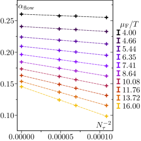
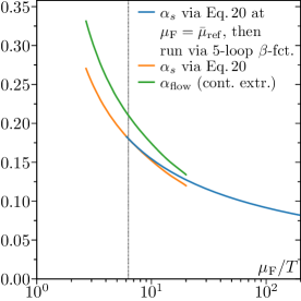
Figure 1: Left: gradient flow coupling $\alpha_{\text{flow}}$ as a function of squared lattice spacing (or equivalently $N_{\tau}^{-2}$ at fixed temperature $T=1/(aN_{\tau})$) at selected flow scales $\mu_{\mathrm{F}}$ in temperature units. The dashed lines correspond to linear fits at fixed flow scale, yielding the continuum-extrapolated data points at $N_{\tau}^{-2}=0$. Statistical errors are smaller than the data line widths. Right: continuum-extrapolated flow coupling $\alpha_{\text{flow}}$ and matched $\overline{\text{MS}}$ coupling $\alpha_{s}$ (via Eq. 20) as a function of gradient flow scale $\mu_{\mathrm{F}}$ in temperature units. Note that the couplings and scales are defined such that $\mu_{\mathrm{F}}=\bar{\mu}$. The dotted vertical line is located at $\mu_{\mathrm{F}}=\bar{\mu}_{\mathrm{ref}}$ (Eq. 21) and depicts the point from where we move to other scales via the perturbative beta function. Statistical errors are smaller than the line width.

                  

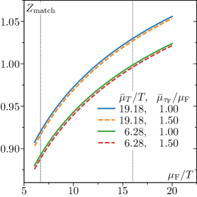
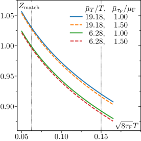
Figure 2: The renormalization factor of the color-magnetic correlator, $Z_{\mathrm{match}}$ (Section II), as a function of flow scale $\mu_{\mathrm{F}}$ in temperature units (left) or as a function of flow radius $\sqrt{8\tau_{F}}$ in inverse temperature units (right) for the four combinations of $\bar{\mu}_{T}$ and $\bar{\mu}_{\tau_{F}}$ defined in Section II. Statistical errors are smaller than the line width. The difference between the panels is the inverted x-axis since $\mu_{\mathrm{F}}=1/(\sqrt{8\tau_{\mathrm{F}}})$.

In order to make use of Section II and the matching procedure explained in Section II, the gauge coupling has to be known in the range from $\bar{\mu}_{\tau_{F}}$ to $\bar{\mu}_{T}$. We can determine the $\overline{\text{MS}}$ gauge coupling $g^{2}_{\overline{\text{MS}}}=4\pi\alpha_{s}$ self-consistently from the lattice data over a range of scales from about $\mu=1/a$ to about $\mu=\pi T$ by evaluating the squared field strength $E=\,\mathrm{Tr}\>G_{\mu\nu}G_{\mu\nu}/2$ under gradient flow, which yields

$$\alpha_{\text{flow}}(\mu_{\mathrm{F}})\equiv\frac{4\pi}{3}\tau_{\mathrm{F}}^{2}\langle E\rangle_{\tau_{\mathrm{F}}}\,.$$ (19)

Then we use the relation between this quantity and the $\overline{\text{MS}}$ coupling, calculated at NLO by Lüscher Lüscher (2010b) and at NNLO by Harlander and Neumann Harlander and Neumann (2016):

$$\alpha_{\text{flow}} =\alpha_{s}\left(1+k_{1}\alpha_{s}+k_{2}\alpha_{s}^{2}\right)\quad\mbox{for}\;\bar{\mu}^{2}=\mu_{\mathrm{F}}^{2}\,,$$ (20)

$$k_{1} =1.098+0.008n_{f}\,,$$

$$k_{2} =-0.982-0.070n_{f}+0.002n_{f}^{2}\,.$$

The $\overline{\text{MS}}$ coupling $\alpha_{s}$ is then obtained by solving the cubic equation. This approach becomes unreliable for $\tau_{\mathrm{F}}<a^{2}$ (where $a$ means lattice spacing) due to missing $\mathcal{O}(a^{2}/\tau_{\mathrm{F}})$ effects. It also has problems when $\tau_{\mathrm{F}}$ becomes too large, as the matching then occurs in a stronger-coupled regime where the perturbative match of Eq. 20 becomes less precise. This makes it difficult to establish $\alpha_{s}$ directly over the full range from $\bar{\mu}_{T}$ to $\bar{\mu}_{\tau_{F}}$. Therefore the best procedure appears to be to use this direct determination at a single value $\mu_{\mathrm{F}}=1/\sqrt{8\tau_{\mathrm{F}}}=\bar{\mu}_{\mathrm{ref}}$ where both lattice-spacing and perturbative effects are under control, and to use the perturbative running of the gauge coupling to obtain it in the desired range. This is the approach we will follow in this work.

                  

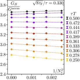
Figure 3: Bare color-magnetic correlator $G_{B}$, tree-level improved and normalized to its free counterpart $G^{\text{norm}}$, as a function of squared lattice spacing $a^{2}$ (or equivalently $1/N_{\tau}^{2}$ at fixed temperature $T=1/(aN_{\tau})$) at the smallest (left) and largest (right) flow time in units of $\sqrt{8\tau_{\mathrm{F}}}/\tau$ according to Eq. 24. The dashed lines and data points at $1/N_{\tau}^{2}=0$ represent the linear-in-$a^{2}$ continuum extrapolation. Statistical errors are smaller than the error bar line width.

Since the matching procedure is conducted based on the continuum theory, it is necessary to extrapolate the flowed coupling constant $\alpha_{\mathrm{flow}}(\mu_{\mathrm{F}})$ measured on the lattice (see Table 2) to the continuum first. Given that the discretization error of the lattice action is of order $a^{2}$, we adopt an Ansatz linear in $a^{2}$. This extrapolation is shown in the left panel of Fig. 1. It can be seen that the Ansatz describes the lattice data well for all relevant flow times. However, the figure shows that the continuum correction is only small for $\mu_{\mathrm{F}}\lesssim 8T$, correspondingly restricting the choice for $\bar{\mu}_{\mathrm{ref}}$. In the right panel of Fig. 1, the continuum-extrapolated $\alpha_{\mathrm{flow}}(\mu_{\mathrm{F}})$ is shown as a solid green curve. Converting it to $\alpha_{\mathrm{s}}$ via Eq. 20 yields the solid orange curve. We select

$$\bar{\mu}_{\mathrm{ref}}\equiv 2\pi T$$ (21)

and have checked that reducing this value by half does not significantly alter the results. From this point we can move to other scales via the perturbative beta function. In practice, the evolution is calculated using the function crd.AlphasExact($\alpha_{s}(\bar{\mu}_{\mathrm{ref}})$, $\bar{\mu}_{\mathrm{ref}}$, $\bar{\mu}_{\tau_{F}}$, $n_{f}=0$, $N_{\mathrm{loop}}=5$) of the RunDec package Herren and Steinhauser (2018); Chetyrkin et al. (2000). The resulting coupling is then used to compute $Z_{\mathrm{match}}$ via Section II, which we show in Fig. 2 for different choices of $\bar{\mu}_{T}$ and $\bar{\mu}_{\tau_{F}}$. The vertical dotted lines enclose all flow times we will use when extrapolating to zero flow (the flow time extrapolation window), meaning that the renormalization procedure changes the bare correlator by at most between $-15\%$ and $+5\%$. We can also see that the difference between choices for $\bar{\mu}_{\tau_{F}}$ is almost negligible, while for $\bar{\mu}_{T}$ the difference is simply a constant multiplicative factor. The four curves for $Z_{\mathrm{match}}$ shown in this figure, which formally differ from each other at the NNLO level, will be used in the next section to obtain four physical correlators via Section II. These will be treated on an equal footing in the spectral analysis and therefore contribute to the overall systematic uncertainty. However, as we will see later, the impact of the different choices on the determination of $\kappa_{B}$ is almost negligible. For this reason, some figures are simplified to show only the choice $(\bar{\mu}_{\tau_{F}}=\bar{\mu}_{\tau_{F},\mathrm{NLO}};\>\bar{\mu}_{T}=\bar{\mu}_{T,\mathrm{NLO}})$.

V Correlator computation

We calculate the color-magnetic correlator $G_{B}$ on the lattice using four different lattice spacings $a$ (cf. Table 1) and perform bootstrap resampling to carry out the complete analysis procedure (i.e., continuum extrapolation, renormalization and flow time extrapolation of $G_{B}$, and in the next section spectral reconstruction) on 1000 bootstrap samples.

Note that to suppress discretization errors, we tree-level improve Meyer (2009) the bare correlator by multiplying it with the ratio of the free correlator obtained in the continuum at leading order $G_{B}^{\mathrm{norm}}(\tau)$ Caron-Huot et al. (2009a) (which is same as in the color-electric case) and the one calculated in lattice perturbation theory at leading order at finite flow time Altenkort et al. (2023)

$$G_{B}^{\rm{latt}}(\tau,\tau_{\mathrm{F}})\rightarrow G_{B}^{\rm{latt}}(\tau,\tau_{\mathrm{F}})\times\frac{G_{B}^{\mathrm{norm}}(\tau)}{G_{B}^{\begin{subarray}{l}{\textrm{\tiny norm}}\\[-0.90417pt] \textrm{\tiny latt}\end{subarray}}(\tau,\tau_{\mathrm{F}})}.$$ (22)

This is equivalent to including tree-level lattice-spacing errors in both the correlator and gradient flow procedures. To make the subtle features of the data visible, we further normalize it by $G_{B}^{\mathrm{norm}}(\tau)$. The quantity of interest is therefore the tree-level improved ratio

$$\frac{G_{B}^{\rm{latt}}(\tau,\tau_{\mathrm{F}})}{G_{B}^{\begin{subarray}{l}{\textrm{\tiny norm}}\\[-0.90417pt] \textrm{\tiny latt}\end{subarray}}(\tau,\tau_{\mathrm{F}})}.$$ (23)

For simplicity we drop the trivial subscript “latt” in the following.

V.1 Continuum extrapolation of the bare correlator

                  

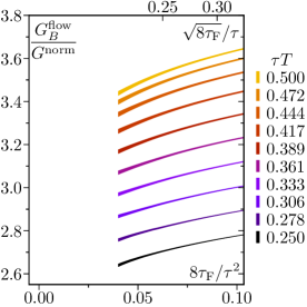
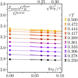
Figure 4: Left: bare continuum-extrapolated color-magnetic correlator $G_{B}$, tree-level improved and normalized to its free counterpart $G^{\text{norm}}$, as a function of normalized flow time $\tau_{\mathrm{F}}/\tau$ for Euclidean temporal separations $\tau$ in units of inverse temperature. The bands depict the statistical $\pm 1\sigma$ error around the median value. Right: the same as on the left, but renormalized by multiplying with $Z_{\mathrm{match}}$ (Section II) for the case $\bar{\mu}_{T}=\bar{\mu}_{T,\mathrm{NLO}}$, $\bar{\mu}_{\tau_{F}}=\bar{\mu}_{\tau_{F},\mathrm{NLO}}$ (other choices differ only marginally or by a simple rescaling). The dashed lines depict the linear-in-$\tau_{\mathrm{F}}/\tau^{2}$ flow time extrapolation, which, due to large autocorrelation between subsequent flow times, is based solely on the three explicit data points indicated between $0.25\leq\sqrt{8\tau_{\mathrm{F}}}/\tau\leq 0.30$ (Eq. 24).

In this section we consider the continuum extrapolation of the bare correlators (Item 2 of Section II). The continuum extrapolation of $G_{B}(\tau,\tau_{\mathrm{F}})/G_{B}^{\mathrm{norm}}(\tau,\tau_{\mathrm{F}})$ requires an interpolation of the Euclidean temporal separations $\tau T$ to the same values across all lattices (we use those present on the finest lattice). This is done using cubic splines with natural boundary condition at the smallest $\tau T$ and zero slope at $\tau T=0.5$ due to the periodic boundary conditions used in the lattice simulation. The continuum extrapolation is carried out using an Ansatz linear in $a^{2}$ as we use the standard Wilson action.

In the two panels of Fig. 3 we show the extrapolation at the minimum and maximum flow time (in units of $\sqrt{8\tau_{\mathrm{F}}}/\tau$, cf. Eq. 24) that is later used in the flow-time-to-zero extrapolation. We can see that the linear-in-$a^{2}$ fit Ansatz gives a good description for the lattice data at all $\tau T$ considered (smaller $\tau T$ are not reliably accessible by the gradient flow method, as explained further below). The continuum-extrapolated results are shown in the left panel of Fig. 4. The renormalized correlators obtained via Section II are shown in the right panel of Fig. 4 as colorful bands. It can be seen that the matching factor does ameliorate the logarithmic flow time divergence, rendering the remaining flow time dependence of the renormalized color-magnetic correlator linear, which is in close resemblance to the behavior of the color-electric correlator (cf. Refs. Altenkort et al. (2021, 2023)).

V.2 Flow-time-to-zero extrapolation of renormalized correlator

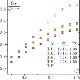
Figure 5: Comparison of renormalized, continuum, zero flow time color-electric ($X=E$, from Ref. Altenkort et al. (2021)) and color-magnetic ($X=B$, this work) correlators as a function of Euclidean temporal separation $\tau$ in inverse temperature units. For the color-magnetic case four variants are shown that arise from the renormalization due to a priori unknown scales at NLO as detailed in Section II.

Now we perform the $\tau_{\mathrm{F}}\rightarrow 0$ extrapolation of the contiuum color-magnetic correlator, which has been renormalized via Section II using the matching factors shown in Fig. 2. As detailed in a previous study of the color-electric field correlators Altenkort et al. (2021, 2023), there is a small flow time window that is usable for the flow extrapolation, which reads:

$$0.25\leq\frac{\sqrt{8\tau_{\mathrm{F}}}}{\tau}\leq 0.3.$$ (24)

The lower limit effectively results from the largest lattice spacing used in the continuum extrapolation, as enough flow needs to be applied to sufficiently suppress lattice discretization artifacts. The upper limit results from a perturbative study Eller and Moore (2018) that allowed the flowed (color-electric) correlator to deviate from its zero flow counterpart by, at most, 1%. This ensures that the flowed correlator does not stray too far from the physical, zero flow time value. Due to Eq. 24, the correlator can only be calculated reliably for Euclidean time separations $\tau T\geq 0.25$.

In the window given by Eq. 24 a linear extrapolation is performed, inspired by the lowest order small flow time expansion and justified by our data. Such a simple Ansatz turns out to work very well as the right panel of Fig. 4 indicates, where the fits, indicated by the dashed lines, go through all data points in the flow time window. We perform this extrapolation by fitting to the three explicitly shown data points at the minimum, midpoint, and maximum of our flow-time window. We do this because there is a large autocorrelation between nearby flow times. Fitting to many nearby flow times is therefore not justified statistically. It is also important that we determine the error in the fit based on the different fit results found in bootstrap resamplings of our data, rather than through naive regression.

In Fig. 5 we show a comparison of the double-extrapolated color-electric field correlator $G_{E}$ from Ref. Altenkort et al. (2021) and the color-magnetic field correlators $G_{B}^{\text{phys.}}$ obtained in this study at the same temperature using the same lattices. The figure shows that each correlator is larger at $\tau T=0.5$ than at small $\tau T$ values. This is partly a result of infrared, thermal contributions to the spectral function, and partly because of the intrinsic separation dependence of the vacuum correlation function. For $G_{E}$ these arise because $G_{E}\propto g^{2}$ which is scale dependent and becomes smaller at short distances – hence the falloff in $G_{E}$ between, say, $\tau T=0.35$ and $\tau T=0.25$. For $G_{B}$ this distance dependence arises from $g^{2}$ and also from the scale (and hence $\tau$) dependence of $Z_{\mathrm{match}}$, or equivalently of $c_{B}^{2}$ as we will discuss around Eq. 26. This softens the $\tau$ dependence of the vacuum $G_{B}$ correlator in comparison to $G_{E}$.

VI spectral reconstruction

                  

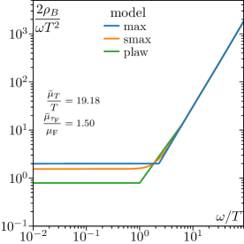
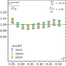
Figure 6: Left: Fitted model spectral functions $\rho_{B}$ as a function of frequency $\omega$ in temperature units for the case $\bar{\mu}_{T}=\bar{\mu}_{T,\mathrm{NLO}}$, $\bar{\mu}_{\tau_{F}}=\bar{\mu}_{\tau_{F},\mathrm{NLO}}$ (other choices differ only marginally). Statistical errors are not shown to reduce clutter; the intent of the figure is to show the differences in spectral function model shapes. The y-axis is scaled to yield $\kappa_{B}/T^{3}$ for $\omega\rightarrow 0$. Right: Ratio of fitted model correlators $G^{\mathrm{model}}$ to renormalized, continuum, zero flow time correlator data $G_{B}$ (cf. Fig. 5) as a function of Euclidean time $\tau$ for the case $\bar{\mu}_{T}=\bar{\mu}_{T,\mathrm{NLO}}$, $\bar{\mu}_{\tau_{F}}=\bar{\mu}_{\tau_{F},\mathrm{NLO}}$ (other choices differ only marginally). Different models are slightly offset in $\tau T$ for visibility.

In this section we invert Eq. 5 to reconstruct the spectral function from the renormalized color-magnetic field correlators $G_{B}^{\text{phys.}}$ obtained above. We model the spectral function consisting of two main parts: the ultraviolet (UV) part and the infrared (IR) part. The UV part is known at both leading order (LO) Banerjee et al. (2022) and next-to-leading order (NLO) Banerjee et al. (2022). At LO the $\overline{\text{MS}}$ spectral function matches the color-electric case and reads

$$\phi^{\mathrm{LO}}_{\rm{UV}}(\omega;\bar{\mu}_{\omega})=\frac{g^{2}(\bar{\mu}_{\omega})C_{F}\omega^{3}}{6\pi},$$ (25)

with $C_{F}=(N_{c}^{2}-1)/(2N_{c})$, $N_{c}=3$ and $g^{2}$ the $\overline{\text{MS}}$ coupling, which should be evaluated at some scale which may be $\omega$ dependent. In a previous paper Altenkort et al. (2024) we use this LO spectral function for the UV point, picking a renormalization point which transitions from a fixed value in the IR to $\bar{\mu}=2\omega$ in the UV. However, this approach is not really self-consistent, since it takes into account one source of NLO logarithmic scale dependence, the running of the coupling, without taking into account another source of logarithmic scale dependence, the renormalization of the $B$-field operators. This operator renormalization also causes a logarithmically scale-dependent shift which is not captured by using an RG-flowed $g^{2}$ value in Eq. 25. Therefore, in this work we will only study the case where the UV is modeled by the NLO spectral function.

The NLO expression for the spectral function in the pure-glue theory is Banerjee et al. (2022)

$$\phi^{\mathrm{NLO}}_{\mathrm{UV}}(\omega;\bar{\mu}_{\omega})= c_{B}^{2}(\bar{\mu}_{\omega},\bar{\mu}_{T})\left(\frac{g^{2}(\bar{\mu}_{\omega})C_{F}\omega^{3}}{6\pi}\left\{1+\frac{N_{c}g^{2}(\bar{\mu}_{\omega})}{(4\pi)^{2}}\left(\frac{5}{3}\ln\frac{\bar{\mu}_{\omega}^{2}}{4\omega^{2}}+\frac{134}{9}-\frac{2\pi^{2}}{3}\right)\right\}+\frac{g^{4}C_{F}}{12\pi^{3}}\left\{\cdots\right\}\right),$$

$$c_{B}^{2}(\mu,\bar{\mu}_{T})= \exp\left(\int_{\bar{\mu}_{T}^{2}}^{\mu^{2}}\gamma_{0}g^{2}(\mu)\frac{\mathrm{d}\mu^{2}}{\mu^{2}}\right).$$ (26)

Note that, compared to Ref. Banerjee et al. (2022), we have corrected the term $-8\pi^{2}/3$ to $-2\pi^{2}/3$. The expression $g^{4}C_{F}/12\pi^{3}(\ldots)$ in Eq. 26, which we have not completely written, is the thermal contribution; the remainder of the expression is the vacuum spectral function. The expression for the thermal contribution is lengthy, but it turns out to be tiny compared to the vacuum contribution when $\omega\gg T$. At very small frequencies $\omega<T$ it is not reliable and in any case small compared to the infrared contribution which the data requires us to add. We include the thermal part but have checked numerically that it has only a marginal effect on the spectral reconstruction.

The quantity in parenthesis on the first line of Eq. 26 represents the $\overline{\text{MS}}$ spectral function. This should be converted to the spectral function for the physical correlator to account for the renormalization of the magnetic field operators on the Wilson line. This necessitates the factor $c_{B}^{2}$, which plays the same role as $Z_{\mathrm{match}}$ played in Section II and in particular in Eq. 11. Including this factor, the expression in Eq. 26 is formally independent of the renormalization scale $\bar{\mu}_{\omega}$ up to NNLO effects, since the explicit logarithm in the first line cancels with the implicit $\mu$ dependence from the 1-loop running of $g^{2}(\bar{\mu}_{\omega})$ and the $\mu$ dependence of $c_{B}^{2}$. Nevertheless, we have to choose some value, and we should attempt to pick a value which will somehow reflect the intrinsic scales present in the spectral function. One such scale is the temperature, and the other is the frequency itself. To estimate the typical thermal scale, we adopt the thermal scale of the dimensionally reduced 3D effective field theory Kajantie et al. (1997),

$$\bar{\mu}_{\mathrm{DR}}=4\pi\exp\left(-\gamma_{E}-\frac{N_{c}-8N_{f}\ln 2}{22N_{c}-4N_{f}}\right)T,$$ (27)

with $N_{c}=3$ and $N_{f}=0$ yielding $\bar{\mu}_{\mathrm{DR}}\approx 6.74T$. This scale should be used for $\omega\sim T$. For the relevant scale at large frequency we use $\bar{\mu}=\omega$, and we transition from one to the other via

$$\bar{\mu}_{\omega}\equiv\sqrt{\omega^{2}+\bar{\mu}_{\mathrm{DR}}^{2}}.$$ (28)

To calculate $c_{B}^{2}$ we also again need the $\overline{\text{MS}}$ coupling constant, which we reuse from Section IV. To take the systematics from higher loop corrections into account we allow a rescaling of the UV part by the fit parameter $K$, that is, we choose $\phi_{\mathrm{UV}}=K\phi^{\mathrm{NLO}}_{\mathrm{UV}}$.

The IR part manifests a very simple structure based on the infrared asymptotics Caron-Huot et al. (2009b):

$$\phi_{\rm{IR}}(\omega)\equiv\frac{\kappa_{B}\omega}{2T}.$$ (29)

Now that both IR and UV parts have been established, the missing link is the region between them. Several schemes have been considered in the literature Francis et al. (2015a); Altenkort et al. (2021); Brambilla et al. (2020); Banerjee et al. (2022); Brambilla et al. (2023); Banerjee et al. (2023); Altenkort et al. (2023). In this study we employ three of them that we consider representative. The first one is simply to take the maximum of the two asymptotics Francis et al. (2015a)

$$\rho_{\rm{max}}\equiv\rm{max}(\phi_{\rm{IR}},\phi_{\rm{UV}}).$$ (30)

The second one makes a smooth switch between the two parts Francis et al. (2015a)

$$\rho_{\rm{smax}}\equiv\sqrt{\phi_{\rm{IR}}^{2}+\phi_{\rm{UV}}^{2}}.$$ (31)

The third one imposes a power-law transition between $\phi_{\rm{IR}}$ and $\phi_{\rm{UV}}$ Brambilla et al. (2020)

$$\begin{split}&\rho_{\mathrm{plaw}}\equiv\begin{cases}\phi_{\mathrm{IR}}&\phantom{\mathrm{for}}\quad\omega\leq\omega_{\mathrm{IR}},\\ p(\omega)&\mathrm{for}\quad\omega_{\mathrm{IR}}<\omega<\omega_{\mathrm{UV}},\\ \phi_{\mathrm{UV}}&\phantom{\mathrm{for}}\quad\omega\geq\omega_{\mathrm{UV}},\\ \end{cases}\\ &p(\omega)=a\omega^{b},\quad a=\frac{\phi_{\mathrm{IR}}(\omega_{\mathrm{IR}})}{(\omega_{\mathrm{IR}})^{b}},\\ &b=\frac{\ln\phi_{\mathrm{IR}}(\omega_{\mathrm{IR}})-\ln\phi_{\mathrm{UV}}(\omega_{\mathrm{UV}})}{\ln\omega_{\mathrm{IR}}-\ln\omega_{\mathrm{UV}}}.\end{split}$$ (32)

The choice for the cuts $\omega_{\mathrm{IR}}$ and $\omega_{\mathrm{UV}}$ can be justified based on some physical arguments. Common option of $\omega_{\mathrm{IR}}$ ranges from $T$ Kajantie et al. (1997) to $\pi T$ Gubser (2008). However, according to Ref. Altenkort et al. (2021), $\rho_{\rm{max}}$ and $\rho_{\rm{smax}}$ also tend to exhibit a transition around $\pi T$. This makes the choice $\pi T$ redundant so we use $\omega_{\mathrm{IR}}=T$. As for $\omega_{\mathrm{UV}}$ we choose $2\pi T$, which is the standard thermal scale obtained from the perturbation theory in the $\overline{\mathrm{MS}}$-scheme Kajantie et al. (1997).

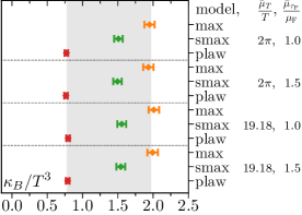
Figure 7: Coefficient $\kappa_{B}$ of the finite-mass correction to heavy-quark momentum diffusion from each model. The grey band shows the confidence interval that ranges from the 34th to 68th percentile of the total distribution of the fit results of all bootstrap samples for all models (see Section V).

With these models we fit the lattice data by minimizing

$$\chi^{2}\equiv\sum_{\tau}\bigg{[}\frac{G_{B}(\tau)-G^{\textrm{model}}(\tau)}{\delta G_{B}(\tau)}\bigg{]}^{2},$$ (33)

where $\delta G_{B}(\tau)$ denotes the error of the lattice data and $G^{\textrm{model}}(\tau)$ is calculated using the convolution (Eq. 5) replacing $\rho_{B}$ by the above models. The two free parameters of the spectral function models are $K$ and $\kappa_{B}/T^{3}$.

Putting the fit results for $\kappa_{B}/T^{3}$ from various models together, we obtain a scatter plot, shown in Fig. 7. We remark that all the fit procedures in this study are performed on each of the 1000 bootstrap samples separately, with the individual fits using inverse squared statistical errors employed as weights. All models describe the lattice data well according to the residual $\chi^{2}$/d.o.f., which is $1.8\pm 0.8$ for $\rho_{\mathrm{max}}$, $1.6\pm 0.8$ for $\rho_{\mathrm{smax}}$ and $1.2\pm 0.7$ for $\rho_{\mathrm{plaw}}$. There is no meaningful difference in the fit quality between the different choices of $\bar{\mu}_{T}$ and $\bar{\mu}_{\tau_{F}}$. Combining the systematic and statistical errors as explained in Altenkort et al. (2023), one obtains a confidence interval for $\kappa_{B}/T^{3}$, shown as grey band in Fig. 7. Including all four combinations for $\bar{\mu}_{T}$ and $\bar{\mu}_{\tau_{F}}$ yields the final estimate

$$0.78\leq\frac{\kappa_{B}}{T^{3}}\leq 1.97,\quad T=1.5T_{c}.$$ (34)

In Fig. 8 we compare $\kappa_{B}$ obtained in this work (black line) and two other calculations, one using the multilevel method Banerjee et al. (2022) and another also using gradient flow with analytical continuation performed at finite flow depth Brambilla et al. (2023). We find that the results are consistent even though they are calculated in different ways.

In Fig. 9 we collect all existing determinations for $\kappa_{E}$ and $\kappa_{B}$ on the market and plot them logarithmically as a function of $g^{2}(\mu=2\pi T)$. The quenched data for $\kappa_{E}$ is taken from Refs. Francis et al. (2015a); Altenkort et al. (2021); Banerjee et al. (2023); Brambilla et al. (2023, 2020), while the quenched data for $\kappa_{B}$ is taken from Refs. Brambilla et al. (2023); Banerjee et al. (2022) and this work. The full QCD data for $\kappa_{E}$ and $\kappa_{B}$ is taken from Ref. Altenkort et al. (2023) and Ref. Altenkort et al. (2024), respectively. Based on perturbation theory Caron-Huot and Moore (2008), $\kappa$ is expected to be proportional to $g^{4}$. This is despite the UV behavior of the spectral function scaling as $g^{2}$, as shown in Eq. 25. When we fit the data using two different Ansätze, one proportional to $g^{2}$ and the other proportional to $g^{4}$, we find that the former fails to describe the data (red curve) both within the quenched data and in connecting quenched with unquenched data, while the latter fits the data rather well (orange curve) with a residual $\chi^{2}/\mathrm{d.o.f.}=0.36$. This corroborates the validity of the perturbative prediction, which has also recently been used in an out-of-equilibrium study on heavy quark diffusion Du (2023).

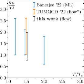
Figure 8: Comparison of quenched $\kappa_{B}/T^{3}$ obtained in this work (including the statistical and systematic uncertainty from all four choices of $\bar{\mu}_{T}$ and $\bar{\mu}_{\tau_{F}}$, as well as the various spectral function models of Section VI) and recent literature. “Banerjee ’22 (ML)” refers to the multilevel method work of Ref. Banerjee et al. (2022), while “TMUQCD ’22 (flow^∗)” refers to Ref. Brambilla et al. (2023), in which gradient flow is used but the spectral reconstruction is performed at finite flow time, indicated by an asterisk in the legend.

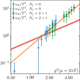
Figure 9: Log-log plot of $\kappa_{E}/T^{3}$ and $\kappa_{B}/T^{3}$ versus the coupling strength $g^{2}(\bar{\mu}=2\pi T)$. The data, from Refs. Francis et al. (2015a); Altenkort et al. (2021); Banerjee et al. (2023); Brambilla et al. (2023, 2020, 2023); Banerjee et al. (2022) and this work, follows a single trend and turns out to fit well to a function proportional to $g^{4}$, given by $\kappa/T^{3}=0.4(0.03)g^{4}$ (orange curve, with the band being the error). The red curve shows an unsuccessful fit of form $\kappa/T^{3}\propto g^{2}$. The fit results are consistent with the perturbative picture that suggests $\kappa/T^{3}\propto g^{4}$ Caron-Huot and Moore (2008).

VII results and conclusions

In this paper we calculate the mass correction to the heavy quark momentum diffusion coefficient using quenched lattice simulations. The correction is extracted from the color-magnetic field correlation functions measured under gradient flow. In our opinion the most interesting part of this paper is Section II, in which we elaborate how to take care of the anomalous dimension existing for a magnetic field operator that is further complicated by the matching from the gradient flow scheme to its physical value. By introducing a matching factor $Z_{\mathrm{match}}$, we establish a multi-step routine that bridges the gap between the object measured under gradient flow and its physical counterpart. $\kappa_{B}$ obtained from the physical correlation functions in this work is consistent with previous quenched results calculated in different ways. We also find that $\kappa_{E,B}$ calculated on the lattice, in both the quenched and the unquenched case, follows a form $\kappa/T^{3}=0.4g^{4}(\bar{\mu}=2\pi T)$ that shows the same scaling with the coupling strength as the perturbative calculation does Caron-Huot and Moore (2008). This remarkably simple expression describes all quenched and unquenched lattice results with a good $\chi^{2}$. The methodology developed in this work can be used in the future for a full QCD study at the physical pion mass reaching lower temperatures around the crossover region.

References

- Collins and Perry (1975) J. C. Collins and M. J. Perry, Phys. Rev. Lett. 34, 1353 (1975).
- Adams et al. (2005) J. Adams et al. (STAR), Nucl. Phys. A 757, 102 (2005), arXiv:nucl-ex/0501009 .
- Arsene et al. (2005) I. Arsene et al. (BRAHMS), Nucl. Phys. A 757, 1 (2005), arXiv:nucl-ex/0410020 .
- Beraudo et al. (2018) A. Beraudo et al., Nucl. Phys. A 979, 21 (2018), arXiv:1803.03824 [nucl-th] .
- Dong and Greco (2019) X. Dong and V. Greco, Prog. Part. Nucl. Phys. 104, 97 (2019).
- He et al. (2023) M. He, H. van Hees, and R. Rapp, Prog. Part. Nucl. Phys. 130, 104020 (2023), arXiv:2204.09299 [hep-ph] .
- Moore and Teaney (2005) G. D. Moore and D. Teaney, Phys. Rev. C 71, 064904 (2005), arXiv:hep-ph/0412346 .
- Caron-Huot and Moore (2008) S. Caron-Huot and G. D. Moore, Phys. Rev. Lett. 100, 052301 (2008), arXiv:0708.4232 [hep-ph] .
- van Hees and Rapp (2005) H. van Hees and R. Rapp, Phys. Rev. C 71, 034907 (2005), arXiv:nucl-th/0412015 .
- Mustafa (2005) M. G. Mustafa, Phys. Rev. C 72, 014905 (2005), arXiv:hep-ph/0412402 .
- Casalderrey-Solana and Teaney (2006) J. Casalderrey-Solana and D. Teaney, Phys. Rev. D74, 085012 (2006), arXiv:hep-ph/0605199 [hep-ph] .
- Caron-Huot et al. (2009a) S. Caron-Huot, M. Laine, and G. D. Moore, JHEP 04, 053 (2009a), arXiv:0901.1195 [hep-lat] .
- Francis et al. (2015a) A. Francis, O. Kaczmarek, M. Laine, T. Neuhaus, and H. Ohno, Phys. Rev. D 92, 116003 (2015a), arXiv:1508.04543 [hep-lat] .
- Altenkort et al. (2021) L. Altenkort, A. M. Eller, O. Kaczmarek, L. Mazur, G. D. Moore, and H.-T. Shu, Phys. Rev. D 103, 014511 (2021), arXiv:2009.13553 [hep-lat] .
- Brambilla et al. (2020) N. Brambilla, V. Leino, P. Petreczky, and A. Vairo (TUMQCD Collaboration), Phys. Rev. D 102, 074503 (2020).
- Banerjee et al. (2023) D. Banerjee, S. Datta, R. V. Gavai, and P. Majumdar, Nuclear Physics A 1038, 122721 (2023).
- Altenkort et al. (2023) L. Altenkort, O. Kaczmarek, R. Larsen, S. Mukherjee, P. Petreczky, H.-T. Shu, and S. Stendebach (HotQCD), Phys. Rev. Lett. 130, 231902 (2023), arXiv:2302.08501 [hep-lat] .
- Bouttefeux and Laine (2020) A. Bouttefeux and M. Laine, JHEP 12, 150 (2020), arXiv:2010.07316 [hep-ph] .
- Banerjee et al. (2022) D. Banerjee, S. Datta, and M. Laine, JHEP 08, 128 (2022), arXiv:2204.14075 [hep-lat] .
- Brambilla et al. (2023) N. Brambilla, V. Leino, J. Mayer-Steudte, and P. Petreczky (TUMQCD), Phys. Rev. D 107, 054508 (2023), arXiv:2206.02861 [hep-lat] .
- Altenkort et al. (2024) L. Altenkort, D. de la Cruz, O. Kaczmarek, R. Larsen, G. D. Moore, S. Mukherjee, P. Petreczky, H.-T. Shu, and S. Stendebach (HotQCD Collaboration), Phys. Rev. Lett. 132, 051902 (2024).
- Laine (2021) M. Laine, JHEP 06, 139 (2021), arXiv:2103.14270 [hep-ph] .
- Narayanan and Neuberger (2006) R. Narayanan and H. Neuberger, JHEP 03, 064 (2006), arXiv:hep-th/0601210 [hep-th] .
- Lüscher (2010a) M. Lüscher, Commun. Math. Phys. 293, 899 (2010a), arXiv:0907.5491 [hep-lat] .
- Lüscher (2010b) M. Lüscher, JHEP 08, 071 (2010b), [Erratum: JHEP03,092(2014)], arXiv:1006.4518 [hep-lat] .
- Lüscher and Weisz (2011) M. Lüscher and P. Weisz, JHEP 02, 051 (2011), arXiv:1101.0963 [hep-th] .
- Brambilla and Wang (2023) N. Brambilla and X.-P. Wang, “Off-lightcone wilson-line operators in gradient flow,” (2023), arXiv:2312.05032 [hep-ph] .
- Harlander and Neumann (2016) R. V. Harlander and T. Neumann, JHEP 06, 161 (2016), arXiv:1606.03756 [hep-ph] .
- Sommer (1994) R. Sommer, Nucl. Phys. B 411, 839 (1994), arXiv:hep-lat/9310022 .
- Francis et al. (2015b) A. Francis, O. Kaczmarek, M. Laine, T. Neuhaus, and H. Ohno, Phys. Rev. D 91, 096002 (2015b), arXiv:1503.05652 [hep-lat] .
- Burnier et al. (2017) Y. Burnier, H. T. Ding, O. Kaczmarek, A. L. Kruse, M. Laine, H. Ohno, and H. Sandmeyer, JHEP 11, 206 (2017), arXiv:1709.07612 [hep-lat] .
- Ramos and Sint (2016) A. Ramos and S. Sint, Eur. Phys. J. C 76, 15 (2016), arXiv:1508.05552 [hep-lat] .
- Mazur et al. (2023) L. Mazur et al., (2023), arXiv:2306.01098 [hep-lat] .
- Altenkort et al. (2022) L. Altenkort, D. Bollweg, D. A. Clarke, O. Kaczmarek, L. Mazur, C. Schmidt, P. Scior, and H.-T. Shu, PoS LATTICE2021, 196 (2022), arXiv:2111.10354 [hep-lat] .
- Mazur (2021) L. Mazur, Topological Aspects in Lattice QCD, Ph.D. thesis, Bielefeld U. (2021).
- Altenkort (2024) L. Altenkort, “correlators_flow public code repository,” (2024).
- Herren and Steinhauser (2018) F. Herren and M. Steinhauser, Comput. Phys. Commun. 224, 333 (2018), arXiv:1703.03751 [hep-ph] .
- Chetyrkin et al. (2000) K. G. Chetyrkin, J. H. Kuhn, and M. Steinhauser, Comput. Phys. Commun. 133, 43 (2000), arXiv:hep-ph/0004189 .
- Meyer (2009) H. B. Meyer, JHEP 06, 077 (2009), arXiv:0904.1806 [hep-lat] .
- Eller and Moore (2018) A. M. Eller and G. D. Moore, Phys. Rev. D97, 114507 (2018), arXiv:1802.04562 [hep-lat] .
- Kajantie et al. (1997) K. Kajantie, M. Laine, K. Rummukainen, and M. E. Shaposhnikov, Nucl. Phys. B 503, 357 (1997), arXiv:hep-ph/9704416 .
- Caron-Huot et al. (2009b) S. Caron-Huot, M. Laine, and G. D. Moore, JHEP 04, 053 (2009b), arXiv:0901.1195 [hep-lat] .
- Gubser (2008) S. S. Gubser, Nucl. Phys. B 790, 175 (2008), arXiv:hep-th/0612143 .
- Du (2023) X. Du, (2023), arXiv:2306.02530 [hep-ph] .