Tuning to the Edge of the Abyss in SU(5)

Abstract

I show that if a dimensionless parameter is tuned to be close to the boundary of the positivity domain and symmetry breaking is driven by a cubic term in the Lagrangian, the physical scale of symmetry breaking in a quantum field theory as measured by the Higgs mass can be much greater than the dimensional scales in the classical Lagrangian. Radiative corrections produce large and physically important corrections, helping to stabilize the large VEV. I describe how this mechanism might produce the GUT scale in an SU(5) model.

Dimensional analysis is one of our simplest and most powerful tools. But there are situations in which it can be confusing if used uncritically. In this note, I show that in a field theory in which a dimensionless parameter can be tuned close to the boundary of the positivity domain, a cubic term in the Lagrangian can produce symmetry breaking in which the physically relevant scales (like the Higgs mass) are parametrically larger than the dimensional scales in the classical Lagrangian. This is not exactly a failure of dimensional analysis because there is a small dimensionless parameter measuring the distance to the boundary. But because we may be interested in theories with very large ratios of physical scales, it seems interesting enough to explore further.

For a renormalizable Lagrangian, the classical positivity domain is the region of the space of dimensionless parameters for which the quartic potential of scalar fields $\phi$ is positive definite so that the potential is positive for large $|\phi|$. On the boundary of the positivity domain, some homogeneous combination of components of $\phi$ vanishes as a coupling $\lambda\to 0$. If we are very near that boundary, the quartic potential depends very weakly on that combination. Then cubic terms in the potential may push the minimum to very negative values for large $|\phi|$ so that some components of the VEV are parametrically large compared to the dimensional parameters, with the Higgs mass and other physical parameters going to infinity as we go to the boundary. Cubic terms are crucial.

Before I describe the model, it will be helpful to explain why the standard model is not such an example. In a doublet Higgs model with quartic coupling $\lambda$ and negative mass squared $-m^{2}$, the VEV squared is $v^{2}\propto|m^{2}|/\lambda$ which goes to $\infty$ as $\lambda\to 0$. However the Higgs mass squared is $\propto\lambda v^{2}\propto|m^{2}|$ which remains fixed as $\lambda$ gets small. For a light Higgs, the partial unification of the weak and electromagnetic interactions occurs at the Higgs scale, not the scale of $v$ or $m_{W}$. This is easiest to see in a renormalizable gauge. Below the Higgs scale, with the Higgs integrated out, the Goldstone bosons are apropriately described by a nonlinear effective chiral theory, but the scale of the higher order terms is set by the Higgs mass, not by the 1TeV scale we would expect in a strongly interacting theory. Above the mass of a light Higgs, the Goldstone bosons look like fundamental scalar fields.

In the mechanism I will describe, the symmetry breaking is driven not by a negative mass-squared term ($m^{2}$ can be positive or zero), but by a cubic term in the Lagrangian with coefficient $\kappa$ with dimensions of mass rather than mass squared. As a coupling $\lambda$ goes to zero, the VEV of a field goes like $v\propto\kappa/\lambda$ and the tree-level Higgs mass goes to $\infty$ as $\lambda\to 0$ like $\kappa/\sqrt{\lambda}$ for fixed $\kappa$ so there is a genuine large scale in the theory. And there are even heavier particles with mass $\propto|\kappa|/\lambda$, which are important in the radiative corrections.

When I decided to investigate this mechanism, I rather expected that quantum corrections would drastically change things. And indeed, I find that the leading quantum corrections are large. But they actually stabilize the vacuum with the large VEV.

I believe that this mechanism can be applied to many models with trilinear couplings and multiple quartic couplings. A relatively simple example where a mechanism to produce a large VEV might be physically interesting is an SU(5) gauge theory [2] with a 24 of scalars. In the conventional picture, the large VEV of the 24 is generated by a conventional Higgs mechanism with a negative mass-squared term of the order of the square of the GUT scale. But in fact, we can tune close to the abyss and let the vacuum do this job with no large dimensional parameters in the Lagrangian. Take $\phi$ to be a hermitian, traceless 5$\times$5 matrix, and write the most general invariant potential

$$\begin{array}[]{c}V(\phi)=\frac{3\lambda_{14}}{50}\Bigl{(}30\mathop{\rm Tr}\nolimits(\phi^{4})-7\mathop{\rm Tr}\nolimits(\phi^{2})^{2}\Bigr{)}\\ +\frac{3\lambda_{23}}{100}\Bigl{(}13\mathop{\rm Tr}\nolimits(\phi^{2})^{2}-20\mathop{\rm Tr}\nolimits(\phi^{4})\Bigr{)}\\ +\sqrt{\frac{10}{3}}\,\kappa\mathop{\rm Tr}\nolimits(\phi^{3})+\frac{m^{2}}{2}\mathop{\rm Tr}\nolimits(\phi^{2})\end{array}$$ (1)

This has the required cubic interaction and $\lambda_{14}$ and $\lambda_{23}$ define the domain of positivity. The coefficients of $\lambda_{14}$ and $\lambda_{23}$ are both positive semi-definite. The $\lambda_{14}$ term vanishes when

$$\begin{array}[]{c}\phi\propto U\,\beta_{23}\,U^{\dagger}\mbox{~{}~{}where~{}~{}}\\ {[\beta_{23}]}_{jk}\equiv\frac{1}{\sqrt{30}}\left(2\delta_{jk}-5(\delta_{j4}\delta_{k4}+\delta_{j5}\delta_{k5})\right)\end{array}$$ (2)

for some unitary $U$. The $\lambda_{23}$ term vanishes when

$$\begin{array}[]{c}\phi\propto U\,\beta_{14}\,U^{\dagger}\mbox{~{}~{}where~{}~{}}\\ {[\beta_{14}]}_{jk}\equiv\frac{1}{\sqrt{30}}\left(\delta_{jk}-5\delta_{j5}\delta_{k5}\right)\end{array}$$ (3)

Thus positivity requires $\lambda_{14}>0$ and $\lambda_{23}>0$ and if one of these two couplings becomes very small, the $\kappa$ term drives the corresponding component of $\phi$ to a very large VEV. For very small coupling, the effect of the mass term is very small, and a non-zero mass complicates the formulas enormously, so for pedagogical reasons we will take $m=0$ in the rest of the paper. This is not a renormalizable constraint because $m^{2}$ depends on the renormalization scale which we will discuss later. But it simplifies the formulas without making any essential difference for small $\lambda$.

In this limit, the VEV is either (2) or (3). The results are summarized below.

$$\begin{array}[]{c}V(\phi_{23}\beta_{23})=\frac{1}{12}\,\phi_{23}^{3}(3\lambda_{23}\phi_{23}-4\,\kappa)\\ \braket{\phi_{23}}=\frac{\kappa}{\lambda_{23}}\quad\quad V(\braket{\phi_{23}}\beta_{23})=-\frac{\kappa^{4}}{12\lambda_{23}^{3}}\rule{0.0pt}{8.61108pt}\end{array}$$ (4)

$$\begin{array}[]{c}V(\phi_{14}\beta_{14})=\frac{1}{4}\phi_{14}^{3}(3\lambda_{14}\phi_{14}-2\sqrt{6}\,\kappa)\\ \braket{\phi_{14}}=\sqrt{\frac{3}{2}}\,\frac{\kappa}{\lambda_{14}}\quad\quad V(\braket{\phi_{14}}\beta_{14})=-\frac{9\kappa^{4}}{16\lambda_{14}^{3}}\rule{0.0pt}{6.45831pt}\end{array}$$ (5)

In the application to GUTs we would like to have $\lambda_{23}<2^{2/3}\lambda_{14}/3$ so that the $\beta_{23}$ vacuum is picked out and the symmetry breaks to SU(3)$\times$SU(2)$\times$U(1). We will discuss this case in detail. The potential $V(\phi_{23}\beta_{23})$ has an inflection point at $\phi_{23}=0$ and for $\kappa>0$ and small $\lambda_{23}$, there is a deep minimum at $\kappa/\lambda_{23}$ as shown in figure 1.

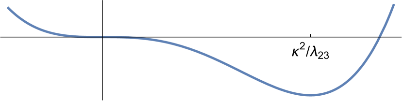
Figure 1: The shape of the tree-level potential

For non-zero real $m$, the inflection point splits (barely noticeably for small $\lambda_{23}$) into a shallow local minimum at $\phi_{23}=0$ and a weak local maximum for $\phi_{23}$ of order $m^{2}/\kappa$ which stays fixed and irrelevant when $\lambda_{23}\to 0$ as the deep minimum moves out to infinity.

Then the massive particles in the theory are the $(3,2)$ of leptoquark gauge bosons, the Higgs scalar $(1,1)$ and the adjoint scalars transforming like $(8,1)$ and $(1,3)$ under SU(3)$\times$SU(2). Their tree-level masses for small $\lambda_{23}$ are

$$\begin{array}[]{|c|c|c|c|}\hline\cr(3,2)&(1,1)&(8,1)&(3,1)\\ \hline\cr\displaystyle\frac{g\kappa}{\lambda_{23}}&\rule[-12.91663pt]{0.0pt}{34.44434pt}\displaystyle\frac{\kappa}{\sqrt{\lambda_{23}}}&\displaystyle\sqrt{\frac{6\lambda_{14}}{5}}\,\frac{\kappa}{\lambda_{23}}&\displaystyle\sqrt{\frac{6\lambda_{14}}{5}}\,\frac{2\kappa}{\lambda_{23}}\rule[-12.91663pt]{0.0pt}{34.44434pt}\\ \hline\cr\end{array}$$ (6)

where $g$ is the gauge coupling. All have masses that go to infinity as $\lambda_{23}\to\infty$ for fixed $\kappa$, but at different rates! The smaller mass for the Higgs multiplet would be very interesting if it persisted beyond tree level because it would be an intermediate mass scale, but I will argue that the one loop corrections modify this quantitative detail while leaving intact the important qualitative feature of large physical masses in the small $\lambda_{23}$ limit.

We can address the quantitative issue using the background field method a la Coleman-Weinberg (CW) [4] and constructing the CW potential as a function of $\phi_{23}$. The SU(3)$\times$SU(2) ensures that the other fields in (6) will be eigenstates of the $\phi_{23}$ dependent “mass” that appears in the CW calculation.

The CW contribution to the potential is

$$\frac{1}{64\pi^{2}}\sum_{j=1}^{4}n_{j}M_{j}(s_{23})^{4}\log\frac{M_{j}(s_{23})^{2}}{\mu^{2}}$$ (7)

where $\mu$ is an arbitrary renormalization scale and $n_{j}$ is the degeneracy of the multiplet. The $M_{j}$ and $n_{j}$ are shown in Table 1.

$$\begin{array}[]{|c|c|c|c|}\hline\cr j&\mbox{type}&n_{j}&M_{j}(\phi_{23})^{2}\\ \hline\cr 1&\mbox{(3,2)}&36*&g^{2}\,\phi_{23}^{2}\\ 2&\mbox{(1,1)}&1&\phi_{23}(3\lambda_{23}\phi_{23}-2\kappa)\\ 3&\mbox{(8,1)}&8&\phi_{23}\bigl{(}(6\lambda_{14}+3\lambda_{23})\phi_{23}+4\kappa\bigr{)}\\ 4&\mbox{(1,3)}&3&3\phi_{23}\bigl{(}(8\lambda_{14}-\lambda_{23})\phi_{23}-10\kappa\bigr{)}/5\\ \hline\cr\lx@intercol\hfil\mbox{*There are 12 color-flavor states, each with 3 spins.}\hfil\lx@intercol\end{array}$$

Table 1: The $\phi_{23}$-dependent masses that appear in (7)

Taking a cue from [4], we can simplify the analysis by choosing $\mu$ so that the CW term leaves the VEV at its classical value. This requires

$$\log\mu^{2}=\frac{\sum_{j}n_{j}M_{j}^{2}(a){M_{j}^{2}}^{\prime}(a)\left(\log M_{j}^{2}(a)+1/2\right)}{\sum_{j}n_{j}M_{j}^{2}(a){M_{j}^{2}}^{\prime}(a)}$$ (8)

In the small $\lambda_{23}$ limit, this gives a $\mu$ of the order of the mass of the heaviest particles (scalar or gauge boson).

The resulting CW contribution to the effective potential can be much larger than the tree level contribution but it further stabilizes the tree-level vacuum. For some typical parameters, an example is shown in figure 2.

Figure 2: $\Re(V_{\rm eff}(\phi_{23})$ including the CW contribution (solid line) for $\lambda_{14}=0.3$, $\lambda_{23}=0.001$, $\kappa=1$, and $m=0$. The dashed line is tree-level. The dotted line is $10^{4}\times\Im(V_{\rm eff})$.

The general shape of the corrections is easy to understand from (7) and Table 1. All of the $M_{j}(\phi_{23})^{2}$ are proportional to $\phi_{23}$ (this is exact in our approximation of $m^{2}=0$, but in general the $M_{j}(\phi_{23})^{2}$ are all small at $\phi_{23}=0$). And they are $\propto\phi_{23}^{2}$ for large $\phi_{23}$. This means that the CW contribution has at least an approximate quadratic zero at the origin. This is a local maximum because the logs are negative. By construction the CW contribution has an extremum at $\phi_{23}=\kappa/\lambda_{23}$. And because of the two $\phi_{23}$s in the mass squares, it grows like $\phi_{23}^{4}$ at large $\phi_{23}$. The minimum scales like $\kappa^{4}/\lambda_{23}^{4}$, so for sufficiently small $\lambda_{23}$, it dominates the tree-level contribution. One can think of figure 2 approximately as a symmetric CW potential

$$\propto\phi^{4}\Bigl{(}\log(\phi^{2}/\mu^{2})-1/2\Bigr{)}$$ (9)

tilted by the effect of the cubic term.

This also means that the CW contribution to the Higgs mass squared scales like $\kappa^{2}/\lambda_{23}^{2}$ and for sufficiently small $\lambda_{23}$ will overwhelm the tree level contribution that scales like $\kappa^{2}/\lambda_{23}$, so the scale of symmetry breaking scales with $\kappa/\lambda_{23}$ like the scalar and massive gauge boson masses. The CW contribution to the Higgs mass squared for small $\lambda_{23}$ is

$$\frac{9(25g^{4}+56\lambda_{14}^{2})\kappa^{2}}{\lambda_{23}^{2}}$$ (10)

Because the CW contribution to the Higgs mass is so large, one might worry that higher order contributions will continue to grow and the loop expansion will be useless. I do not expect this to happen. The CW contribution is larger than the tree-level for very small $\lambda_{23}$ because it scales with an extra power of the VEV. Higher loop contributions will have the same dimensional scaling and so will be suppressed by small dimensionless coupling constants, as usual in perturbation theory.

It is a long way from this toy SU(5) model to a realistic GUT. Because the symmetry-breaking mechanism is different, some model-building issues will have to be solved in new and different ways. But I hope that I have convinced the reader that this mechanism for symmetry breaking with cubic terms and small couplings at the edge of the positivity domain is a possible alternative to the conventional scheme. I don’t believe that this solves the tuning problem in GUTs, but it might replace the usual tuning problem with a very different one. And I somehow just like the idea that some of the puzzles in fundamental physics might arise because our world is perched precariously near the edge of oblivion.

References

- Note [1] We will see below that radiative corrections make the physical Higgs mass larger, scaling like the heavier particle masses.
- Georgi and Glashow [1974] H. Georgi and S. L. Glashow, Unity of All Elementary Particle Forces, Phys. Rev. Lett. 32, 438 (1974).
- Note [2] This model has been studied for over 50 years, and it is possible that the mechanism I describe has been discussed somewhere in the extensive literature on the subject. If so, I apologize for missing it and I assume that the authors will enlighten me.
- Coleman and Weinberg [1973] S. R. Coleman and E. J. Weinberg, Radiative Corrections as the Origin of Spontaneous Symmetry Breaking, Phys. Rev. D 7, 1888 (1973).