Eulerian Formulation of the Tensor-Based Morphology Equations for Strain-Based Blood Damage Modeling

Abstract

The development of blood-handling medical devices, such as ventricular assist devices, requires the analysis of their biocompatibility. Among other aspects, this includes hemolysis, i.e., red blood cell damage. For this purpose, computational fluid dynamics (CFD) methods are employed to predict blood flow in prototypes. The most basic hemolysis models directly estimate red blood cell damage from fluid stress in the resulting flow field. More advanced models explicitly resolve cell deformation. On the downside, these models are typically written in a Lagrangian formulation, i.e., they require pathline tracking. We present a new Eulerian description of cell deformation, enabling the evaluation of the solution across the whole domain. The resulting hemolysis model can be applied to any converged CFD simulation due to one-way coupling with the fluid velocity field. We discuss the efficient numerical treatment of the model equations in a stabilized finite element context. We validate the model by comparison to the original Lagrangian formulation in selected benchmark flows. Two more complex test cases demonstrate the method’s capabilities in real-world applications. The results highlight the advantages over previous hemolysis models. In conclusion, the model holds great potential for the design process of future generations of medical devices.

[CATS] organization=Chair for Computational Analysis of Technical Systems
RWTH Aachen University, addressline=Schinkelstr. 2, city=52062 Aachen, country=Germany

[ILSB]organization=Institute of Lightweight Design and Structural Biomechanics
TU Wien, addressline=Gumpendorfer Str. 7, city=A-1060 Vienna, country=Austria

1 Introduction

As the prevalence of heart failure continues to rise worldwide [1], the development of blood handling medical devices, such as ventricular assist devices, has become paramount in improving patient outcomes and extending life expectancy. Such devices are generally characterized by partly conflicting indicators of performance. Hydraulic performance, on the one hand, quantifies the pressure head and the resulting flow rates and encourages high fluid stress. Hematologic performance, on the other hand, quantifies the damage to the constituent components of blood and calls for low fluid stress. A critical challenge in the development process is thus to balance these aspects. Nowadays, the development process is supported by CFD. It allows for a comprehensive understanding of how the design and operating parameters of a VAD influence the device’s hydraulic performance. The hematologic assessment requires additional methods and usually involves analysis of the device’s potential for hemolysis, i.e., red blood cell (RBC) damage, among other aspects.

Hemolysis occurs when the hemoglobin contained within an RBC leaks out into blood plasma. While this can have various causes, we focus on mechanical hemolysis in the context of blood-handling medical devices. In mechanical hemolysis, fluid stresses induce excessive cell deformation, which can damage the cell membrane or even lead to cell rupture. Modeling mechanical hemolysis has been subject of intense research over the past 40 years [2, 3, 4, 5, 6, 7]. Despite these efforts, there is still no universally accepted approach. In fact, a recent comparison has shown that computational predictions are still frequently inaccurate [8]. This uncertainty, in combination with new findings on the clinical significance of hemolysis [9], calls for the development of more reliable hemolysis models. Existing models can be categorized as stress-based models and strain-based models.

Stress-based hemolysis models apply an empirical correlation for hemoglobin release directly to the instantaneous fluid stress field. This approach has two downsides. First, such models assume implicitly that cells immediately deform to their steady state when encountering stress. This is because empirical hemolysis correlations are generally measured at constant stress, i.e., the cell has time to adapt to this level of stress and reach a steady state. When encountering changing levels of stress, however, the cell membrane exhibits viscoelastic behavior [10]. This means that short, high levels of stress may not lead to significant hemolysis if the membrane does not have sufficient time to stretch in response. Stress-based models assume that the full instantaneous fluid stress applies immediately. Second, it is unclear how the correlation should be applied to arbitrary three-dimensional stress states. The empirical correlations [3, 11] generally only relate shear stress to hemoglobin release. One generalization to arbitrary stress states was proposed by Bludszuweit [4]. She defined a scalar stress that results from a weighted sum of the stress components. However, the reduction to a representative scalar loses some information of the three-dimensional stress state, as a cell experiences different loads depending on its alignment with the principal axes of stress. In particular, Goldsmith and Marlow [12] showed that cells tend to align more with the flow direction at higher shear rates. More recently, it was suggested [13, 14] that for certain flows, extensional stresses have a larger effect on cell deformation than shear stresses. Overall, the proper weighting of the stress components is still unclear and may depend on the flow regimes at hand. For these reasons, a first-principles model that explicitly describes cell deformation as a result of flow forces is preferable.

Strain-based hemolysis models incorporate such cell deformation models into hemolysis prediction. The empirical correlations for hemoglobin release are then applied to the causative membrane strain itself. There are different degrees of complexity for the cell deformation model. On the simpler side, Chen and Sharp [15] proposed a scalar model for estimating membrane strain in the context of cell rupture. However, this model was not originally intended for predicting sublethal hemolysis [16] and failed to achieve satisfactory results for this purpose [17]. Arwatz and Smits [18] described a scalar viscoelastic model for cell deformation. Its real-world applicability is limited, though, as it does not account for the complex three-dimensional flow forces and it was formulated only for constant shear flow. Thus, simple strain-based models tend to be valid only for specific applications.

On the more complex side, Ezzeldin et al. [19] and Sohrabi and Liu [20] developed models that resolve the cell membrane’s three-dimensional deformation. Porcaro and Saeedipour [21] employed a reduced-order model for the cell structure and modeled the cells’ interaction with the flow and with each other. Moreover, there exists a wide array of cell deformation models that were not specifically intended for hemolysis prediction but could be used in this context [22, 23, 24, 25, 26, 27]. These complex approaches resolve cell deformation using varying degrees of freedom and achieve varying levels of computational performance. Nevertheless, they all have in common that their computational cost is too high to simulate large-scale VADs. Modern devices support flow rates of up to $10\,\frac{\mathrm{L}}{\mathrm{min}}$ [28], corresponding to almost 1 trillion RBCs per second. This means that in these models, generally only a small fraction of all cells are chosen at the inlet of the device and tracked until the outlet. Hemolysis is then averaged over these cells. This approach has two disadvantages. First, it is unclear how to pick the cells to achieve a representative average. Second, it gives a global index for hemolysis, but does not highlight critical regions inside the domain. In particular, it cannot be guaranteed that the selected cells will penetrate every part of the domain, e.g., boundary layers and recirculation areas. In conclusion, such complex cell deformation models are not well suited to aid the design process of VADs.

The aim of the present work is to develop a new model that combines the advantages of the different classes of models described above: the efficiency of stress-based and simple strain-based models, the characteristic cell response to three-dimensional stress of more complex strain-based models, and an Eulerian description, enabling evaluation across the entire domain.

For this purpose, the strain-based model by Arora et al. [5] serves as basis, as it provides a compromise between these degrees of complexity, approximating RBCs as three-dimensional ellipsoids. However, it is based on a Lagrangian description of particle motion. In consequence, its evaluation requires particle tracking and comes with the same drawbacks as the more complex cell deformation models described above. Pauli et al. [6] introduced an Eulerian formulation. In the process, they neglected part of the model to achieve this formulation. As we will show in the present work, this may generally not be an admissible simplification in many situations. Instead, we will derive a full-order Eulerian formulation that is analytically equivalent to the original model. In addition, we will present a modification to improve robustness and efficiency, thus making the model suitable for simulations of realistic VAD configurations.

The paper is structured as follows: In Section 2, we define the constitutive equations for our strain-based hemolysis model. We introduce the original Lagrangian model formulation and derive the new full-order Eulerian formulation, contrasting it with the previous Eulerian formulation. In addition, we present a novel model with improved efficiency and robustness. In Section 3 we discuss how we treat the model equations numerically using our in-house multiphysics solver. In Section 4, we show results for validation and benchmarking. Finally, we summarize our work, discuss the model’s limitations and give an outlook on future research in Section 5.

2 Model Equations

At rest, red blood cells are known to aggregate into stacks, so-called rouleaux. Under shear, these structures break up and the cells move through the flow in a tumbling motion. At even higher shear rates, cells stop tumbling and start to assume a fixed orientation. In this state, their shape resembles elongated ellipsoids, with their major axis aligned with the flow direction [29, 12]. This motion has been termed tank-treading, as the cell membrane rotates around the cell contents like the treads of a tank [30]. This regime of high shear rates is of primary interest for hemolysis modeling.

In this section, we present different models to describe RBCs in this regime. In Section 2.1, we introduce the original Lagrangian model formulation that constitutes the basis for all further discussion. In Section 2.2, we derive an equivalent Eulerian formulation. In Section 2.3, we present a new model that effectively replicates the original model behavior with better numerical performance. Finally, we contrast this with an older Eulerian model formulation in Section 2.4. In strain-based hemolysis modeling, any of these RBC models may be used to compute a scalar parameter that serves as input to empirical hemolysis correlations. This process is described in Section 2.5.

2.1 Lagrangian model formulation

(a) Morphology $\bm{\mathbf{S}}$ with eigenvalues $\lambda_{i}$ and eigenvectors $\bm{\mathbf{v}}_{i}$

(b) Eigenvector rotation $\bm{\mathbf{\Omega}}$

(c) Recovery source term

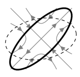
(d) Strain source term

(e) Vorticity source term

Figure 1: Ellipsoidal cell representation in Arora morphology model

Based on the fluid droplet model by Maffettone and Minale [31], Arora et al. [5] derived a Lagrangian cell deformation model. Thereby, RBCs are assumed as neutrally bouyant ellipsoidal droplets carried with the flow. Ellipsoids can be described mathematically by a symmetric positive definite morphology tensor $\bm{\mathbf{S}}$, whose eigenvalues $\lambda_{i}$ represent the squared lengths of the ellipsoid’s semi-axes. In this work, they are assumed to be in descending order, i.e., $\lambda_{1}\geq\lambda_{2}\geq\lambda_{3}$. Due to volume conservation, their product has to remain constant. The eigenvectors $\bm{\mathbf{v}}_{i}$ represent the orientation of the ellipsoid’s semi-axes. They can be understood as a rotation matrix $\bm{\mathbf{Q}}=[\bm{\mathbf{v}}_{1},\bm{\mathbf{v}}_{2},\bm{\mathbf{v}}_{3}]$ that rotates the global inert coordinate system to the local rotating coordinate system of the cell. As derived in Appendix A, the rotation rate of the local frame with respect to the inertial frame is quantified by the rotation tensor

$$\bm{\mathbf{\Omega}}=\frac{\mathrm{d}\bm{\mathbf{Q}}}{\mathrm{d}t}\bm{\mathbf{Q}}^{\mathbf{T}}\,.$$ (1)

The cells in the Arora model [5] do not interact with one another and do not influence the flow field. The evolution equation for the morphology of a single cell may be written along its pathline as follows:

$$\frac{\mathrm{d}\bm{\mathbf{S}}}{\mathrm{d}t}-\mathopen{}\mathclose{{}\left[\bm{\mathbf{\Omega}},\,\bm{\mathbf{S}}}\right]=-f_{1}\mathopen{}\mathclose{{}\left(\bm{\mathbf{S}}-g\mathopen{}\mathclose{{}\left(\bm{\mathbf{S}}}\right)\bm{\mathbf{I}}}\right)+f_{2}\mathopen{}\mathclose{{}\left(\bm{\mathbf{E}},\,\bm{\mathbf{S}}}\right)+f_{3}\mathopen{}\mathclose{{}\left[\bm{\mathbf{W}}-\bm{\mathbf{\Omega}},\,\bm{\mathbf{S}}}\right]\,,$$ (2)

with tensor operations $\mathopen{}\mathclose{{}\left[\bm{\mathbf{\Omega}},\,\bm{\mathbf{S}}}\right]\coloneqq\bm{\mathbf{\Omega}}\bm{\mathbf{S}}-\bm{\mathbf{S}}\bm{\mathbf{\Omega}}$ and $\mathopen{}\mathclose{{}\left(\bm{\mathbf{E}},\,\bm{\mathbf{S}}}\right)\coloneqq\bm{\mathbf{E}}\bm{\mathbf{S}}+\bm{\mathbf{S}}\bm{\mathbf{E}}$, and coefficients

$$f_{1}=5.0\,\unit{}^{-1}\,,\qquad f_{2}=f_{3}=4.2298\cdot 10^{-4}\,.$$ (3)

For details on the derivation of these coefficients, see [5]. The first term on the right-hand side describes shape recovery with the scalar function

$$g(\bm{\mathbf{S}})=\frac{6\,\mathrm{det}\bm{\mathbf{S}}}{\mathrm{tr}(\bm{\mathbf{S}})^{2}-\mathrm{tr}\mathopen{}\mathclose{{}\left(\bm{\mathbf{S}}^{2}}\right)}\,.$$

The second term on the right-hand side describes the effect of fluid strain

$$\bm{\mathbf{E}}=\frac{1}{2}\mathopen{}\mathclose{{}\left(\big{(}\bm{\mathbf{\nabla}}\bm{\mathbf{u}}\big{)}+\big{(}\bm{\mathbf{\nabla}}\bm{\mathbf{u}}\big{)}^{\mathbf{T}}}\right)\,,$$

which causes the cell to align with the principal axes of strain and to deform along those axes. The third term on the right-hand side describes the effect of fluid vorticity

$$\bm{\mathbf{W}}=\frac{1}{2}\mathopen{}\mathclose{{}\left(\big{(}\bm{\mathbf{\nabla}}\bm{\mathbf{u}}\big{)}-\big{(}\bm{\mathbf{\nabla}}\bm{\mathbf{u}}\big{)}^{\mathbf{T}}}\right)\,,$$

which rotates the cell. These three effects are combined as linear superposition. The left-hand side of Eq. 2 represents a Jaumann derivative that defines a co-rotating reference frame. Hence, the model employs a Lagrangian description of cell deformation, so its evaluation requires pathline tracking. The components of the model are visualized in Fig. 1.

2.2 Full-order Eulerian morphology model

A direct reformulation of Eq. 2 towards an Eulerian description is challenging due to the implicit dependency between the morphology tensor $\bm{\mathbf{S}}$ and the rotation rate of its eigenvectors $\bm{\mathbf{\Omega}}$. In order to resolve this dependency, we derive an expression for $\bm{\mathbf{\Omega}}$ that does not involve derivatives of $\bm{\mathbf{Q}}$. For this purpose, the spectral decomposition of the morphology tensor

$$\bm{\mathbf{S}}=\bm{\mathbf{Q}}\bm{\mathbf{\Lambda}}\bm{\mathbf{Q}}^{\mathbf{T}}\,,\qquad\bm{\mathbf{\Lambda}}=\bm{\mathbf{diag}}(\lambda_{1},\lambda_{2},\lambda_{3})\,,\qquad\bm{\mathbf{Q}}=[\bm{\mathbf{v}}_{1},\bm{\mathbf{v}}_{2},\bm{\mathbf{v}}_{3}]\,,$$ (4)

is employed. In the following, the model equation 2 is transformed to the eigenbasis of the morphology tensor by multiplying with $\bm{\mathbf{Q}}^{\mathbf{T}}$ from the left and with $\bm{\mathbf{Q}}$ from the right. The transformed quantities are then defined as

$$\tilde{\bm{\mathbf{E}}}=\bm{\mathbf{Q}}^{\mathbf{T}}\bm{\mathbf{E}}\bm{\mathbf{Q}}\,,\qquad\tilde{\bm{\mathbf{W}}}=\bm{\mathbf{Q}}^{\mathbf{T}}\bm{\mathbf{W}}\bm{\mathbf{Q}}\,,\qquad\tilde{\bm{\mathbf{\Omega}}}=\bm{\mathbf{Q}}^{\mathbf{T}}\bm{\mathbf{\Omega}}\bm{\mathbf{Q}}\,.$$ (5)

First, the derivative of the shape tensor $\frac{\mathrm{d}\bm{\mathbf{S}}}{\mathrm{d}t}$ becomes

$$\begin{split}\bm{\mathbf{Q}}^{\mathbf{T}}\frac{\mathrm{d}\bm{\mathbf{S}}}{\mathrm{d}t}\bm{\mathbf{Q}}&=\bm{\mathbf{Q}}^{\mathbf{T}}\frac{\mathrm{d}}{\mathrm{d}t}\mathopen{}\mathclose{{}\left(\bm{\mathbf{Q}}\bm{\mathbf{\Lambda}}\bm{\mathbf{Q}}^{\mathbf{T}}}\right)\bm{\mathbf{Q}}\\ &=\bm{\mathbf{Q}}^{\mathbf{T}}\mathopen{}\mathclose{{}\left(\frac{\mathrm{d}\bm{\mathbf{Q}}}{\mathrm{d}t}\bm{\mathbf{\Lambda}}\bm{\mathbf{Q}}^{\mathbf{T}}+\bm{\mathbf{Q}}\frac{\mathrm{d}\bm{\mathbf{\Lambda}}}{\mathrm{d}t}\bm{\mathbf{Q}}^{\mathbf{T}}+\bm{\mathbf{Q}}\bm{\mathbf{\Lambda}}\frac{\mathrm{d}\bm{\mathbf{Q}}^{\mathbf{T}}}{\mathrm{d}t}}\right)\bm{\mathbf{Q}}\\ &\overset{\eqref{eq:om}}{=}\bm{\mathbf{Q}}^{\mathbf{T}}\bm{\mathbf{\Omega}}\bm{\mathbf{Q}}\bm{\mathbf{\Lambda}}+\frac{\mathrm{d}\bm{\mathbf{\Lambda}}}{\mathrm{d}t}-\bm{\mathbf{\Lambda}}\bm{\mathbf{Q}}^{\mathbf{T}}\bm{\mathbf{\Omega}}\bm{\mathbf{Q}}\\ &=\frac{\mathrm{d}\bm{\mathbf{\Lambda}}}{\mathrm{d}t}+\mathopen{}\mathclose{{}\left[\tilde{\bm{\mathbf{\Omega}}},\,\bm{\mathbf{\Lambda}}}\right]\,.\end{split}$$

Second, the rotation term $\mathopen{}\mathclose{{}\left[\bm{\mathbf{\Omega}},\,\bm{\mathbf{S}}}\right]$ becomes:

$$\begin{split}\bm{\mathbf{Q}}^{\mathbf{T}}\mathopen{}\mathclose{{}\left[\bm{\mathbf{\Omega}},\,\bm{\mathbf{S}}}\right]\bm{\mathbf{Q}}&=\bm{\mathbf{Q}}^{\mathbf{T}}\bm{\mathbf{\Omega}}\bm{\mathbf{S}}\bm{\mathbf{Q}}-\bm{\mathbf{Q}}^{\mathbf{T}}\bm{\mathbf{S}}\bm{\mathbf{\Omega}}\bm{\mathbf{Q}}\\ &=\bm{\mathbf{Q}}^{\mathbf{T}}\bm{\mathbf{\Omega}}\bm{\mathbf{Q}}\bm{\mathbf{Q}}^{\mathbf{T}}\bm{\mathbf{S}}\bm{\mathbf{Q}}-\bm{\mathbf{Q}}^{\mathbf{T}}\bm{\mathbf{S}}\bm{\mathbf{Q}}\bm{\mathbf{Q}}^{\mathbf{T}}\bm{\mathbf{\Omega}}\bm{\mathbf{Q}}\\ &=\tilde{\bm{\mathbf{\Omega}}}\bm{\mathbf{\Lambda}}-\bm{\mathbf{\Lambda}}\tilde{\bm{\mathbf{\Omega}}}\\ &=\mathopen{}\mathclose{{}\left[\tilde{\bm{\mathbf{\Omega}}},\,\bm{\mathbf{\Lambda}}}\right]\,.\end{split}$$

Third, the same transformation is applied to the right-hand side of Eq. 2 in analogous fashion to obtain the full transformed model:

$$\frac{\mathrm{d}\bm{\mathbf{\Lambda}}}{\mathrm{d}t}=-f_{1}\mathopen{}\mathclose{{}\left(\bm{\mathbf{\Lambda}}-g\mathopen{}\mathclose{{}\left(\bm{\mathbf{\Lambda}}}\right)\bm{\mathbf{I}}}\right)+f_{2}\mathopen{}\mathclose{{}\left(\tilde{\bm{\mathbf{E}}},\,\bm{\mathbf{\Lambda}}}\right)+f_{3}\mathopen{}\mathclose{{}\left[\tilde{\bm{\mathbf{W}}}-\tilde{\bm{\mathbf{\Omega}}},\,\bm{\mathbf{\Lambda}}}\right]\,.$$ (6)

Because $\tilde{\bm{\mathbf{\Omega}}}$ and $\tilde{\bm{\mathbf{W}}}$ are antisymmetric and $\bm{\mathbf{\Lambda}}$ is diagonal, the last term on the right-hand side contains no elements on the diagonal. This lets us rewrite the equation only for the off-diagonal elements as follows:

$$\mathopen{}\mathclose{{}\left[\tilde{\bm{\mathbf{\Omega}}},\,\bm{\mathbf{\Lambda}}}\right]=\frac{f_{2}}{f_{3}}\mathopen{}\mathclose{{}\left(\tilde{\bm{\mathbf{E}}},\,\bm{\mathbf{\Lambda}}}\right)-\frac{f_{2}}{f_{3}}\bm{\mathbf{diag}}\mathopen{}\mathclose{{}\left(\tilde{\bm{\mathbf{E}}},\,\bm{\mathbf{\Lambda}}}\right)+\mathopen{}\mathclose{{}\left[\tilde{\bm{\mathbf{W}}},\,\bm{\mathbf{\Lambda}}}\right]\,.$$

Here, the $\bm{\mathbf{\bm{\mathbf{diag}}}}$ operator leaves only the diagonal entries and sets all off-diagonal entries to zero. Applying the inverse coordinate transformation yields:

$$\mathopen{}\mathclose{{}\left[\bm{\mathbf{\Omega}},\,\bm{\mathbf{S}}}\right]=\frac{f_{2}}{f_{3}}\mathopen{}\mathclose{{}\left(\bm{\mathbf{E}}-\hat{\bm{\mathbf{E}}},\,\bm{\mathbf{S}}}\right)+\mathopen{}\mathclose{{}\left[\bm{\mathbf{W}},\,\bm{\mathbf{S}}}\right]\,,\quad\hat{\bm{\mathbf{E}}}=\bm{\mathbf{Q}}\,\bm{\mathbf{diag}}\mathopen{}\mathclose{{}\left(\bm{\mathbf{Q}}^{\mathbf{T}}\bm{\mathbf{E}}\bm{\mathbf{Q}}}\right)\bm{\mathbf{Q}}^{\mathbf{T}}\,.$$ (7)

Finally, we obtain the full Eulerian morphology model by treating the morphology tensor $\bm{\mathbf{S}}$ as a field variable, hence understanding the Lagrangian derivative as a material derivative. The expression 7 then allows us to rewrite the original model 2 as follows:

$$\frac{\partial\bm{\mathbf{S}}}{\partial t}+(\bm{\mathbf{u}}\cdot\bm{\mathbf{\nabla}})\bm{\mathbf{S}}=-f_{1}\mathopen{}\mathclose{{}\left(\bm{\mathbf{S}}-g\mathopen{}\mathclose{{}\left(\bm{\mathbf{S}}}\right)\bm{\mathbf{I}}}\right)+f_{2}\mathopen{}\mathclose{{}\left(\hat{\bm{\mathbf{E}}},\,\bm{\mathbf{S}}}\right)+\frac{f_{2}}{f_{3}}\mathopen{}\mathclose{{}\left(\bm{\mathbf{E}}-\hat{\bm{\mathbf{E}}},\,\bm{\mathbf{S}}}\right)+\mathopen{}\mathclose{{}\left[\bm{\mathbf{W}},\,\bm{\mathbf{S}}}\right]\,.$$ (8)

This constitutes an analytically equivalent Eulerian formulation of the original model. Intuitively, $\hat{\bm{\mathbf{E}}}$ represents the component of $\bm{\mathbf{E}}$ that solely acts to deform the cell, computed as a projection on the morphology eigenvectors $\bm{\mathbf{Q}}$. Consequently, $\bm{\mathbf{E}}-\hat{\bm{\mathbf{E}}}$ represents the component of $\bm{\mathbf{E}}$ that solely acts to rotate the cell towards the principal axes of strain. The two different strain components are visualized in Fig. 2.

We remark that there is still an implicit relationship between the morphology tensor $\bm{\mathbf{S}}$ and the deformational strain $\hat{\bm{\mathbf{E}}}$, as the latter is a function of the morphology eigenvectors $\bm{\mathbf{Q}}$. In contrast to the original formulation, however, this formulation does not involve the derivatives of these eigenvectors. The dependency is purely algebraic and can be resolved in the framework of the numerical method, e.g., by means of Newton iterations.

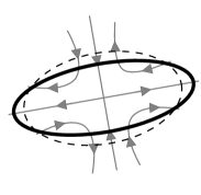
(a) Deformational strain $\hat{\bm{\mathbf{E}}}$

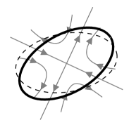
(b) Rotational strain $\bm{\mathbf{E}}-\hat{\bm{\mathbf{E}}}$

Figure 2: Strain terms in full-order Eulerian formulation

2.3 Tank-treading cell deformation model

An approach to resolve this dependency analytically is to rewrite the model explicitly in terms of the eigenvalues and eigenvectors of $\bm{\mathbf{S}}$. For this purpose, we consider the diagonal terms and the off-diagonal terms of Eq. 6 separately and use the definitions 1 and 5:

$$\frac{\partial\lambda_{i}}{\partial t}+(\bm{\mathbf{u}}\cdot\bm{\mathbf{\nabla}})\lambda_{i} =-f_{1}\mathopen{}\mathclose{{}\left(\lambda_{i}-g(\bm{\mathbf{\Lambda}})}\right)+2f_{2}\lambda_{i}\tilde{E}_{ii}\,,$$ (9a)

$$\frac{\partial\bm{\mathbf{Q}}}{\partial t}+(\bm{\mathbf{u}}\cdot\bm{\mathbf{\nabla}})\bm{\mathbf{Q}} =\bm{\mathbf{Q}}\,\tilde{\bm{\mathbf{\Omega}}}(\bm{\mathbf{Q}})\,,\qquad\tilde{\Omega}_{ij}(\bm{\mathbf{Q}})=\frac{f_{2}}{f_{3}}\tilde{E}_{ij}\frac{\lambda_{j}+\lambda_{i}}{\lambda_{j}-\lambda_{i}}+\tilde{W}_{ij}\,.$$ (9b)

Equations 9a and 9b describe the deformation and rotation of cells, respectively. In particular, the deformation equation 9a contains the effects of the recovery term (see Fig. 1(c)) and the deformational strain (see Fig. 2(a)). The terms are transformed to the eigensystem of the morphology tensor to act directly on the eigenvalues $\lambda_{i}$, which represent the ellipsoid’s semi-axes. Similarly, the rotation equation 9b describes the effects of the rotational strain (see Fig. 2(b)) and the vorticity (see Fig. 1(e)) on the eigenvectors $\bm{\mathbf{Q}}=[\bm{\mathbf{v}}_{1},\bm{\mathbf{v}}_{2},\bm{\mathbf{v}}_{3}]$, which represent the ellipsoid’s orientation.

The rotation equation 9b exhibits a singularity at $\lambda_{i}=\lambda_{j}$. This corresponds to a circular cross-section of the ellipsoid, which makes the eigenvectors immediately align with the principal axes of strain in that plane. The eigenvectors may thus be computed as solution to $\tilde{E}_{ij}=0$ in this degenerate state.

The formulation 9 is challenging to solve numerically due to the rotation equation 9b. On the one hand, the rotational source term 9b is three orders of magnitude larger than the deformation source term 9a and can become arbitrarily large due to the singularity at $\lambda_{i}=\lambda_{j}$ This creates a discrepancy of timescales and requires prohibitively small time steps. On the other hand, the orthogonal matrix $\bm{\mathbf{Q}}$ is impractical to handle numerically as a field variable, as it contains 9 entries and its columns need to remain orthonormal. These issues lead to large computational effort and a high number of numerical constraints, making direct numerical simulation unfeasible for realistic geometries.

To alleviate these issues, we derive a model for the behavior of the rotation equation 9b on the slower timescale of the deformation problem. For this purpose, we assume that rotation happens infinitely fast compared to deformation and distinguish between two states: tank-treading and tumbling.

A tank-treading cell assumes steady orientation with the flow. With the given timescale assumptions, this happens effectively instantly, and the orientation is in equilibrium after the initial alignment process. This essentially corresponds to a quasi-steady state assumption on the orientation in the Lagrangian frame, i.e., $\frac{\mathrm{d}\bm{\mathbf{Q}}}{\mathrm{d}t}=\frac{\partial\bm{\mathbf{Q}}}{\partial t}+(\bm{\mathbf{u}}\cdot\bm{\mathbf{\nabla}})\bm{\mathbf{Q}}=\bm{\mathbf{0}}$. Thus, finding the steady orientation means finding $\bm{\mathbf{Q}}$ such that $\tilde{\bm{\mathbf{\Omega}}}=\bm{\mathbf{0}}$ in Eq. 9b. The $\bm{\mathbf{Q}}$ that satisfies this condition is termed $\bm{\mathbf{Q}}_{\mathrm{steady}}$ and depends on the deformation $\bm{\mathbf{\Lambda}}$ and the flow quantities $\bm{\mathbf{E}}$ and $\bm{\mathbf{W}}$.

A tumbling cell is too deformed to assume a steady orientation at the given flow state. In consequence, it will keep rotating and experience tensile and compressional stresses to approximately equal amounts. The source term $\tilde{\bm{\mathbf{E}}}$ in the deformation equation 9a thus tends to zero in the long timescale. This can be ensured by setting $\bm{\mathbf{Q}}=\bm{\mathbf{0}}$.

In sum, the tank-treading morphology model (TTM) becomes:

$$\frac{\partial\lambda_{i}}{\partial t}+(\bm{\mathbf{u}}\cdot\bm{\mathbf{\nabla}})\lambda_{i} =-f_{1}\mathopen{}\mathclose{{}\left(\lambda_{i}-g(\bm{\mathbf{\Lambda}})}\right)+2f_{2}\lambda_{i}\tilde{E}_{ii}\,,\qquad\tilde{\bm{\mathbf{E}}}=\bm{\mathbf{Q}}^{\mathbf{T}}\bm{\mathbf{E}}\bm{\mathbf{Q}}\,,$$ (10a)

$$\bm{\mathbf{Q}} =\begin{dcases}\bm{\mathbf{Q}}_{\mathrm{steady}}(\bm{\mathbf{\Lambda}},\bm{\mathbf{E}},\bm{\mathbf{W}}),&\text{steady orientation exists}\,,\\ \bm{\mathbf{0}},&\text{otherwise}\,.\end{dcases}$$ (10b)

This formulation reduces the rotation equation 9b to an algebraic equation 10b, avoiding the associated time step limitations. The approach to solve the algebraic equation is detailed in Section 2.3.2. Moreover, the deformation equations can be simplified as well; due to volume conservation, the product of the eigenvalues has to remain constant and can be set to unity without loss of generality. Thus, we only need to solve Eq. 10a for $\lambda_{1}$ and $\lambda_{3}$ and can compute $\lambda_{2}=\frac{1}{\lambda_{1}\lambda_{3}}$. This reduces the number of differential variables from six in the full-order model 8 to just two in the TTM 10. As demonstrated in Sections 4.3 and 4.4, this results in significant improvements in efficiency and robustness.

2.3.1 Logarithmic formulation of tank-treading morphology model

For additional robustness, we employ a logarithmic transformation as presented by Haßler et al. [32] to ensure positive eigenvalues in the correct order. We define the following transformation:

$$\lambda_{1}=1+e^{\hat{\lambda}_{1}}\in(1,\infty)\,,\qquad\lambda_{3}=\frac{1}{1+e^{\hat{\lambda}_{3}}}\in(0,1)\,.$$ (11)

We rewrite the material derivative of the deformation model 10a in terms of the transformed eigenvalues:

$$\frac{\partial\hat{\lambda}_{1}}{\partial t}+(\bm{\mathbf{u}}\cdot\bm{\mathbf{\nabla}})\hat{\lambda}_{1} =\frac{\mathcal{F}_{1}(\bm{\mathbf{\Lambda}})}{\lambda_{1}-1}\,,\qquad\frac{\partial\hat{\lambda}_{3}}{\partial t}+(\bm{\mathbf{u}}\cdot\bm{\mathbf{\nabla}})\hat{\lambda}_{3}=\frac{\mathcal{F}_{3}(\bm{\mathbf{\Lambda}})}{\lambda_{3}^{2}-\lambda_{3}}\,,$$ (12)

$$\mathcal{F}_{i}(\bm{\mathbf{\Lambda}}) =-f_{1}\mathopen{}\mathclose{{}\left(\lambda_{i}-g(\bm{\mathbf{\Lambda}})}\right)+2f_{2}\lambda_{i}\tilde{E}_{ii}\,.$$

This is the logarithmic formulation of the tank-treading morphology model (TTLM). The model is thus solved for the transformed eigenvalues $\hat{\lambda}_{1}$ and $\hat{\lambda}_{3}$. The original eigenvalues $\lambda_{1}$ and $\lambda_{3}$ are obtained from the transformation 11. The right-hand side source terms are computed using these original eigenvalues.

2.3.2 Determining the steady orientation of the cell

The algebraic equation 10b requires us to solve the equation $\bm{\mathbf{\Omega}}(\bm{\mathbf{Q}})=\bm{\mathbf{0}}$ or, equivalently, $\tilde{\bm{\mathbf{\Omega}}}(\bm{\mathbf{Q}})=\bm{\mathbf{0}}$. We will derive the solution analytically in 2D first and then generalize it numerically to 3D. Without loss of generality, assume that the two-dimensional rotation happens in the plane normal to the third axis and that $\lambda_{1}\neq\lambda_{2}$ (otherwise the cross-section is circular and the orientation is arbitrary). Then we only need to consider $\bm{\mathbf{E}},\bm{\mathbf{W}},\bm{\mathbf{\Lambda}},\bm{\mathbf{Q}},\bm{\mathbf{\Omega}}\in\mathbb{R}^{2\times 2}$. In particular, the two-dimensional orientation $\bm{\mathbf{Q}}$ can be expressed in terms of a single variable $\theta$:

$$\bm{\mathbf{Q}}(\theta)=\begin{bmatrix}\cos\theta&-\sin\theta\\ \sin\theta&\cos\theta\\ \end{bmatrix}\,.$$

This allows us to write the rotation rate 9b as a function of this scalar $\theta$:

$$\tilde{\Omega}_{21}(\theta;\bm{\mathbf{\Lambda}},\bm{\mathbf{E}},\bm{\mathbf{W}})=\frac{f_{2}}{f_{3}}\frac{\lambda_{1}+\lambda_{2}}{\lambda_{1}-\lambda_{2}}\mathopen{}\mathclose{{}\left(E_{12}\cos(2\theta)+\frac{1}{2}(E_{22}-E_{11})\sin(2\theta)}\right)-W_{12}\,.$$

For ease of notation, we define the coefficients

$$a(\bm{\mathbf{\Lambda}},\bm{\mathbf{E}})\coloneqq\frac{f_{2}}{f_{3}}\frac{\lambda_{1}+\lambda_{2}}{\lambda_{1}-\lambda_{2}}E_{12}\,,\ b(\bm{\mathbf{\Lambda}},\bm{\mathbf{E}})\coloneqq\frac{f_{2}}{2f_{3}}\frac{\lambda_{1}+\lambda_{2}}{\lambda_{1}-\lambda_{2}}(E_{22}-E_{11})\,,\ c(\bm{\mathbf{W}})\coloneqq W_{12}\,.$$

A solution to $\tilde{\Omega}_{21}=0$ exists only if

$$a^{2}+b^{2}\geq c^{2}\,.$$ (13)

This condition weighs the aligning effects of strain against the rotational effects of vorticity. If the vorticity is too strong, the strain cannot keep the cell at a fixed orientation and the cell tumbles instead. If a steady orientation exists, there are always two solutions. We demand that the steady orientation is stable, i.e., the cell returns to the steady orientation after small perturbations. This corresponds to the condition $\frac{\partial\tilde{\Omega}_{21}}{\partial\theta}<0$. We find that the only solution that satisfies this condition is

$$\theta_{\mathrm{steady}}(a,b,c)=\arctan\mathopen{}\mathclose{{}\left(\frac{a+\sqrt{a^{2}+b^{2}-c^{2}}}{b+c}}\right)\,.$$ (14)

This corresponds to the solution where the longest semi-axis of the cell experiences the most tension and the shortest semi-axis experiences the most compression. The steady orientation may then be computed as $\bm{\mathbf{Q}}_{\mathrm{steady}}=\bm{\mathbf{Q}}(\theta_{\mathrm{steady}})$.

Next, we will derive an approach to apply this analytical solution in a three-dimensional setting, i.e., $\bm{\mathbf{E}},\bm{\mathbf{W}},\bm{\mathbf{\Lambda}},\bm{\mathbf{Q}},\bm{\mathbf{\Omega}}\in\mathbb{R}^{3\times 3}$. In order to map three-dimensional states to the two-dimensional setting considered above, we define the projection operator

$$\bm{\mathbf{\mathcal{P}}}_{k}:\mathbb{R}^{3\times 3}\to\mathbb{R}^{2\times 2}\,,\quad\bm{\mathbf{\mathcal{P}}}_{k}(\bm{\mathbf{A}})=(A_{ij})_{i\neq k,\\ j\neq k}\,.$$

It projects the three-dimensional state to the two-dimensional plane normal to the $k$-th coordinate axis. The transformed quantities 5 are written in the eigensystem of the morphology tensor. Thus, projecting them this way gives us information in a plane that contains two of the ellipsoid’s semi-axes $\bm{\mathbf{v}}_{i},i\neq k$. We treat this cross-section according to the two-dimensional findings. This allows us to determine the steady state angle $\theta_{\mathrm{steady}}^{(k)}$ in that cross-section $k$.

The idea for the algorithm is as follows: In order to move towards a steady state, we rotate the three-dimensional ellipsoid within that $k$-th plane by the steady state angle $\theta_{\mathrm{steady}}^{(k)}$. For this purpose, we construct the $k$-th elemental rotation matrix $\bm{\mathbf{R}}_{k}(\theta)$, which represents a rotation by the angle $\theta$ around the $k$-th axis. Then we apply the rotation with $\theta=\theta_{\mathrm{steady}}^{(k)}$ to the current ellipsoid orientation $\bm{\mathbf{Q}}$ from the right. This corresponds to a rotation around the ellipsoid’s $k$-th axis. We iterate over the three axes $k=1,2,3$ and accumulate these rotations until the orientation $\bm{\mathbf{Q}}$ does not change more than some pre-defined threshold. These steps are listed in Algorithm 1.

Input: A cell deformation $\bm{\mathbf{\Lambda}}$, fluid strain $\bm{\mathbf{E}}$ and fluid vorticity $\bm{\mathbf{W}}$

Output: A cell orientation $\bm{\mathbf{Q}}$ for the TTM within an accuracy of $\varepsilon$.

1 $\bm{\mathbf{Q}}\leftarrow\bm{\mathbf{I}}$ ;

2 do

3       $converged\leftarrow true$ ;

4       for $k\leftarrow 1$ to $3$  do

5             $\tilde{\bm{\mathbf{E}}}\leftarrow\bm{\mathbf{Q}}^{\mathbf{T}}\bm{\mathbf{E}}\bm{\mathbf{Q}}\,,\quad\tilde{\bm{\mathbf{W}}}\leftarrow\bm{\mathbf{Q}}^{\mathbf{T}}\bm{\mathbf{W}}\bm{\mathbf{Q}}$ ;

6             $\bm{\mathbf{E}}^{(k)}\leftarrow\bm{\mathbf{\mathcal{P}}}_{k}(\tilde{\bm{\mathbf{E}}})\,,\quad\bm{\mathbf{W}}^{(k)}\leftarrow\bm{\mathbf{\mathcal{P}}}_{k}(\tilde{\bm{\mathbf{W}}})\,,\quad\bm{\mathbf{\Lambda}}^{(k)}\leftarrow\bm{\mathbf{\mathcal{P}}}_{k}(\bm{\mathbf{\Lambda}})$ ;

7             $a_{k}\leftarrow a(\bm{\mathbf{\Lambda}}^{(k)},\bm{\mathbf{E}}^{(k)})\,,\ b_{k}\leftarrow b(\bm{\mathbf{\Lambda}}^{(k)},\bm{\mathbf{E}}^{(k)})\,,\ c_{k}\leftarrow c(\bm{\mathbf{W}}^{(k)})$ ;

8             if $a_{k}^{2}+b_{k}^{2}\geq c_{k}^{2}$ then // cell is tank-treading

9                   $\theta_{k}\leftarrow\theta_{\mathrm{steady}}(a_{k},b_{k},c_{k})$ ;

10                   $\bm{\mathbf{Q}}\leftarrow\bm{\mathbf{Q}}\bm{\mathbf{R}}_{k}(\theta_{k})$ ;

11                   $converged\leftarrow(converged\land|\theta_{k}|\leq\varepsilon)$ ;

12                  

13             else  // cell is tumbling

14                   $\bm{\mathbf{Q}}\leftarrow\bm{\mathbf{0}}$ ;

15                   return ;

16                  

17             end if

18            

19       end for

20      

21while not converged;

Algorithm 1 Steady orientation algorithm in 3D

In case of unstable convergence behavior, an underrelaxation factor may be added to the update of the orientation in line 10. In the underlying study, Algorithm 1 converged for over $99.9\,\%$ of quadrature points, mostly within fewer than 10 iterations of the outer loop. The algorithm converges towards a state where the longest axis of the cell experiences the most tension and the shortest axis experiences the most compression, i.e., $\tilde{E}_{11}\geq\tilde{E}_{22}\geq\tilde{E}_{33}$. This is in agreement with the two-dimensional results. Overall, we find that the algorithm reliably and efficiently produces a unique solution.

An alternative is numerically integrating the transient equation $\frac{\mathrm{d}\bm{\mathbf{Q}}}{\mathrm{d}t}=\bm{\mathbf{Q}}\tilde{\bm{\mathbf{\Omega}}}$ up until steady state. This is computationally inefficient, as it requires on the order of 100,000 time steps and does not allow for the detection of tumbling. It is used only as a fallback solution in case Algorithm 1 does not converge.

2.4 Simplified Eulerian formulation

Previously, another formulation was obtained by Pauli et al. [6] by neglecting the eigenvector rotation $\bm{\mathbf{\Omega}}$ in Eq. 2. This enables a more direct Eulerian description:

$$\frac{\partial\bm{\mathbf{S}}}{\partial t}+(\bm{\mathbf{u}}\cdot\bm{\mathbf{\nabla}})\bm{\mathbf{S}}=-f_{1}\mathopen{}\mathclose{{}\left(\bm{\mathbf{S}}-g\mathopen{}\mathclose{{}\left(\bm{\mathbf{S}}}\right)\bm{\mathbf{I}}}\right)+f_{2}\mathopen{}\mathclose{{}\left(\bm{\mathbf{E}},\,\bm{\mathbf{S}}}\right)+f_{3}\mathopen{}\mathclose{{}\left[\bm{\mathbf{W}},\,\bm{\mathbf{S}}}\right]\,.$$ (15)

Applying the same transformation as in Section 2.2 yields

$$\mathopen{}\mathclose{{}\left[\bm{\mathbf{\Omega}},\,\bm{\mathbf{S}}}\right]=f_{2}\mathopen{}\mathclose{{}\left(\bm{\mathbf{E}}-\hat{\bm{\mathbf{E}}},\,\bm{\mathbf{S}}}\right)+f_{3}\mathopen{}\mathclose{{}\left[\bm{\mathbf{W}},\,\bm{\mathbf{S}}}\right]\,.$$ (16)

The eigenvector rotation rate $\bm{\mathbf{\Omega}}$ is three orders of magnitude smaller than that in the full-order model 7. The simplified model 15 is thus not equivalent to the original formulation. Furthermore, Eq. 16 shows that the simplified model still contains eigenvector rotation, despite initially neglecting the associated terms. These findings indicate that the simplified Eulerian formulation is inconsistent. The effects of this inconsistency will be discussed in Section 4.

2.5 Strain-based hemolysis modeling

Following Arora et al. [5], any of the cell deformation models from above may be employed to compute the cell distortion $D$ and the resulting effective shear rate $G_{\mathrm{eff}}$:

$$D=\frac{\sqrt{\lambda_{1}}-\sqrt{\lambda_{3}}}{\sqrt{\lambda_{1}}+\sqrt{\lambda_{3}}}\,,\qquad G_{\mathrm{eff}}=\frac{2Df_{1}}{(1-D^{2})f_{2}}\,.$$ (17)

This effective shear rate may then serve as input to an empirical correlation relating shear stress to hemoglobin release [3, 11]. The release rate can be interpreted as source term for an advection-diffusion equation that describes the free hemoglobin concentration in the blood. This has been described in detail in previous works [33, 6]. The focus of the present study will be the cell morphology model itself, as it constitutes the defining feature of strain-based blood damage models.

3 Numerical Method

Simulations are carried out using our in-house multiphysics finite element solver. They consist of two components: the flow problem and the morphology problem. The flow problem is solved first and information about the flow field is then transferred to the morphology problem in a one-way coupling. In this section, we first present the mathematical definitions of these two problems in Sections 3.1 and 3.2. The computational framework for Eulerian hemolysis modeling is described in Section 3.3. Finally, we explain the Lagrangian validation procedure in Section 3.4.

3.1 Flow problem

Whole blood is assumed to be an incompressible, Newtonian fluid, which is generally valid for blood at high shear rates [34]. High shear regions are the most significant in this context, since this is where the majority of hemolysis occurs. Fluid flow is thus governed by the incompressible Navier-Stokes equations:

$$\rho\mathopen{}\mathclose{{}\left(\frac{\partial\bm{\mathbf{u}}}{\partial t}+(\bm{\mathbf{u}}\cdot\bm{\mathbf{\nabla}})\bm{\mathbf{u}}}\right) =-\bm{\mathbf{\nabla}}\cdot\bm{\mathbf{\sigma}} \text{in $\mathfrak{D}$}\,,$$

$$\bm{\mathbf{\nabla}}\cdot\bm{\mathbf{u}} =0 \text{in $\mathfrak{D}$}\,,$$

$$\bm{\mathbf{\sigma}} =-p\bm{\mathbf{I}}+2\mu\bm{\mathbf{E}} \text{in $\mathfrak{D}$}\,,$$

$$\bm{\mathbf{u}} =\bm{\mathbf{u}}_{\mathrm{in}} \text{on $\Gamma_{\mathrm{in}}$}\,,$$

$$\bm{\mathbf{u}} =\bm{\mathbf{u}}_{\mathrm{wall}} \text{on $\Gamma_{\mathrm{wall}}$}\,,$$

$$\bm{\mathbf{\sigma}}\cdot\bm{\mathbf{n}} =\bm{\mathbf{0}} \text{on $\Gamma_{\mathrm{out}}$}\,,$$

for the fluid domain $\mathfrak{D}$. The domain boundary $\partial\mathfrak{D}$ is partitioned into inflow $\Gamma_{\mathrm{in}}$, no-slip walls $\Gamma_{\mathrm{wall}}$ and stress-free outflow $\Gamma_{\mathrm{out}}$. As material parameters for blood, we select a density of $\rho=1.054\,\unit{\per\cubic\centi}$ and a viscosity of $3.5\,\mathrm{cP}$. The problem is discretized with stabilized finite elements and solved in steady state, i.e., $\frac{\partial\bm{\mathbf{u}}}{\partial t}=\bm{\mathbf{0}}$. For details on the stabilization terms, we refer to Pauli and Behr [35]. To simulate rotating systems at steady state, we employ the moving reference frame (MRF) approach [36].

3.2 Morphology problem

Fundamentally, the morphology models 8, 10 and 15 represent advection-reaction equations. Aggregating the respective differential degrees of freedom in a vector $\bm{\mathbf{\phi}}$, each of them can be written in the following form:

$$\bm{\mathbf{\mathcal{R}}}_{\mathsf{M}}(\bm{\mathbf{\phi}};\bm{\mathbf{u}},\bm{\mathbf{\nabla}}\bm{\mathbf{u}})\coloneqq\frac{\partial\bm{\mathbf{\phi}}}{\partial t}+(\bm{\mathbf{u}}\cdot\bm{\mathbf{\nabla}})\bm{\mathbf{\phi}}-\bm{\mathbf{f}}(\bm{\mathbf{\phi}},\bm{\mathbf{\nabla}}\bm{\mathbf{u}}) =\bm{\mathbf{0}}\qquad \text{in $\mathfrak{D}$}\,,$$ (18a)

$$\bm{\mathbf{\phi}} =\bm{\mathbf{\phi}}_{\mathrm{in}}\qquad \text{on $\Gamma_{\mathrm{in}}$}\,,$$ (18b)

$$\bm{\mathbf{\nabla}}\bm{\mathbf{\phi}}\cdot\bm{\mathbf{n}} =\bm{\mathbf{0}}\qquad \text{on $\Gamma_{\mathrm{wall}}\cup\Gamma_{\mathrm{out}}$}\,.$$ (18c)

At the inlet $\Gamma_{\mathrm{in}}$, we impose some cell morphology, e.g., an undeformed cell. At walls and at the outflow, there is no component of advection velocity from the boundary into the computational domain. Consequently, we apply no-flux boundary conditions at all remaining boundaries $\Gamma_{\mathrm{wall}}\cup\Gamma_{\mathrm{out}}=\partial\mathfrak{D}\setminus\Gamma_{\mathrm{in}}$.

Similar to the MRF approach for the flow problem, the governing equations for the morphology model are transformed in the relative frame. Given a relative velocity field $\tilde{\bm{\mathbf{u}}}=\bm{\mathbf{u}}-\bm{\mathbf{\Omega}}^{\mathrm{rot}}\times\bm{\mathbf{r}}$, the governing equations are transformed to the relative frame as follows:

$$\bm{\mathbf{\mathcal{R}}}_{\mathsf{M}}(\bm{\mathbf{\phi}};\tilde{\bm{\mathbf{u}}},\bm{\mathbf{\nabla}}\bm{\mathbf{u}}-\bm{\mathbf{\Omega}}^{\mathrm{rot}})=\bm{\mathbf{0}}\qquad\text{in $\mathfrak{D}^{\mathrm{rot}}$}\,.$$

This formulation describes particles being advected with the relative velocity $\tilde{\bm{\mathbf{u}}}$ and incorporates the rotation into the velocity gradient. It holds true for model formulations that are objective, i.e., invariant under rotation. This is the case for models 8 and 10. The simplified model 15 is not objective, however, as cells do not rotate with the full fluid vorticity $\bm{\mathbf{W}}$. This particular model thus requires the addition of another term that accounts for the rotating reference frame:

$$\frac{\partial\bm{\mathbf{S}}}{\partial t}+(\tilde{\bm{\mathbf{u}}}\cdot\bm{\mathbf{\nabla}})\bm{\mathbf{S}}=-f_{1}\mathopen{}\mathclose{{}\left(\bm{\mathbf{S}}-g\mathopen{}\mathclose{{}\left(\bm{\mathbf{S}}}\right)\bm{\mathbf{I}}}\right)+f_{2}\mathopen{}\mathclose{{}\left(\bm{\mathbf{E}},\,\bm{\mathbf{S}}}\right)+f_{3}\mathopen{}\mathclose{{}\left[\bm{\mathbf{W}},\,\bm{\mathbf{S}}}\right]-\mathopen{}\mathclose{{}\left[\bm{\mathbf{\Omega}}^{\mathrm{rot}},\,\bm{\mathbf{S}}}\right]\qquad\text{in $\mathfrak{D}^{\mathrm{rot}}$}\,.$$

For the finite element discretization, we consider the stabilized weak Galerkin formulation of the problem: Find $\bm{\mathbf{\phi}}^{h}\in\mathcal{S}^{h}\subset[H^{1}(\mathfrak{D})]^{n_{\mathrm{dof}}}$ such that:

$$D_{\mathsf{M}}(\bm{\mathbf{\psi}}^{h},\bm{\mathbf{\phi}}^{h})+E_{\mathsf{M}}(\bm{\mathbf{\psi}}^{h},\bm{\mathbf{\phi}}^{h})+J_{\mathsf{M}}(\bm{\mathbf{\psi}}^{h},\bm{\mathbf{\phi}}^{h})=0\qquad\forall\bm{\mathbf{\psi}}^{h}\in\mathcal{V}^{h}\subset[H^{1}_{0}(\mathfrak{D})]^{n_{\mathrm{dof}}}\,,$$ (19)

where $H^{1}(\mathfrak{D})$ denotes the set of functions with square-integrable first derivatives on $\mathfrak{D}$ and $H^{1}_{0}(\mathfrak{D})$ is a subset of those functions satisfying a homogeneous Dirichlet boundary condition on $\Gamma_{\mathrm{in}}$. The first term represents the constitutive model equations:

$$\begin{split}D_{\mathsf{M}}(\bm{\mathbf{\psi}}^{h},\bm{\mathbf{\phi}}^{h})=&\int_{\mathfrak{D}\setminus\mathfrak{D}^{\mathrm{rot}}}\bm{\mathbf{\psi}}^{h}\cdot\bm{\mathbf{\mathcal{R}}}_{\mathsf{M}}(\bm{\mathbf{\phi}}^{h},\bm{\mathbf{u}},\bm{\mathbf{\nabla}}\bm{\mathbf{u}})\,\mathrm{d}\mathfrak{D}\\ +&\int_{\mathfrak{D}^{\mathrm{rot}}}\bm{\mathbf{\psi}}^{h}\cdot\bm{\mathbf{\mathcal{R}}}_{\mathsf{M}}(\bm{\mathbf{\phi}}^{h},\tilde{\bm{\mathbf{u}}},\bm{\mathbf{\nabla}}\bm{\mathbf{u}}-\bm{\mathbf{\Omega}}^{\mathrm{rot}})\,\mathrm{d}\mathfrak{D}\,.\end{split}$$

The second term $E_{\mathsf{M}}$ represents stabilization. We are using Galerkin/least-squares (GLS) stabilization [37]. For details on the formulation for multi-dimensional variables, we refer to Pauli [34]. The third term represents $YZ\beta$ discontinuity capturing [38], computed element by element:

$$J_{\mathsf{M}}(\bm{\mathbf{\psi}}^{h},\bm{\mathbf{\phi}}^{h})=\sum_{e=1}^{n_{\mathrm{el}}}\int_{\mathfrak{D}_{e}}\nu_{\mathrm{DC}}\bm{\mathbf{\nabla}}\bm{\mathbf{\psi}}^{h}:\bm{\mathbf{\nabla}}\bm{\mathbf{\phi}}^{h}\,\mathrm{d}\mathfrak{D}\,.$$

3.3 Implementation

Having explained the theoretical foundations of our approach to Eulerian hemolysis simulation based on the flow and morphology problems, we now turn to its practical implementation by integrating it into our in-house multiphysics finite element code XNS. The latter is written in Fortran and parallelized by the in-house EWD communication library using the Message Passing Interface (MPI). This allows us to exploit the potential of modern high performance computing (HPC) architectures, especially for large-scale problems. XNS supports semi-discrete as well as space-time finite element formulations [35] and entails a number of advanced methods for moving and deforming grids [39, 40, 41, 42]. It also provides capabilities to perform parametric model order reduction [43, 44] using the RBniCS library [45].

The design of XNS adheres to the object-oriented programming (OOP) paradigm. Here, we employ encapsulation to structure the code in a modular fashion, which comes with increased data security and promotes a more intuitive understanding of the code’s design. In particular, the code is organized to separate the numerical discretization aspects, including computational mesh and time discretization, from the formulation of physical field equations and the incorporation of features such as stabilization schemes or discontinuity capturing. Furthermore, the design also facilitates coupling, e.g., between multiple field problems, which requires exchanging the corresponding solution fields. Here, XNS provides functionality to couple field problems both weakly and strongly, according to one-way or mutual dependencies.

The OOP approach also enables the usage of inheritance and polymorphism. On the one hand, inheritance is leveraged throughout the code to create a hierarchy of classes, allowing the derived classes to inherit properties and behaviors from parent classes. Thereby, common functionality can be efficiently implemented by reusing and sharing existing code. For example, the distribution of temperature or concentration can be governed by the same scalar transport equation, but with different material parameters or source terms. Using the concept of inheritance, this unified equation structure allows us to encapsulate the common functionality while still addressing the specific variations.

On the other hand, polymorphism is implemented, enabling objects of different classes to be treated as objects of a common superclass. As an illustrative example, the use of polymorphism allows the assembly process in the finite element procedure to be implemented only once for different field problems derived from a common superclass. This design approach allows seamless interchangeability and coupling of different problem types and avoids code duplication.

The above concepts are also particularly useful in the context of this work. Due to the modular design, it was straightforward to create an additional module for the morphology problem and integrate it into the existing framework of field problems.

All field problems are derived from a common parent class FieldProblemT. The flow problem is implemented as a subclass INSProblemT. For the different Eulerian models from Section 2, we followed the concept of inheritance to reflect their common properties. We introduced a new parent class MorphologyProblemT related to the generic formulation 19. From this, we derived classes for the specific models that differ in number of degrees of freeedom and in definition of the source term. MorphologyTensorProblemT is the parent class for the morphology models that involve the morphology tensor $\bm{\mathbf{S}}$. The full-order model 8 and the simplified model 15 are implemented as subclasses MorphologyFullOrderT and MorphologySimplifiedT, respectively. MorphologyEigProblemT implements the problems that operate directly on the eigenvalues $\lambda_{i}$ of $\bm{\mathbf{S}}$. The TTM from Eq. 10 and the TTLM from Eq. 12 are implemented as subclasses TankTreadingT and TankTreadingLogarithmicT, respectively. Figure 3 gives an overview of the classes and their inheritance.

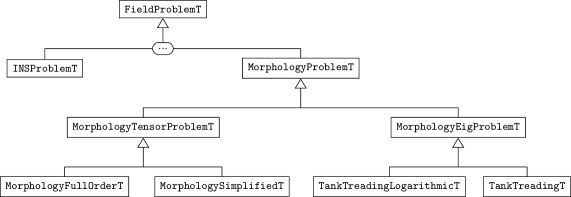
Figure 3: Inheritance structure of Eulerian field problems in XNS.

As has been mentioned above, the flow and morphology problems are coupled in a weak manner. Thereby, the solution of the flow problem, i.e., the velocity field and its gradient, is used in the morphology problem.

3.4 Particle tracing

In order to validate the Eulerian model formulations and their numerical discretization, we compare them to their Lagrangian counterparts. This is achieved in five steps, all of which are available as part of our open-source Python package HemTracer. First, we use the same Eulerian flow field determined by the flow problem (see Section 3.1) to compute pathlines, i.e., trajectories of fluid particles. They are obtained by integrating the following ordinary differential equation (ODE) starting from a given initial position $\bm{\mathbf{X}}_{0}$:

$$\frac{\mathrm{d}\bm{\mathbf{X}}}{\mathrm{d}t}=\begin{dcases}\bm{\mathbf{u}}(\bm{\mathbf{X}},t)\,,&\text{$\bm{\mathbf{X}}(t)\in\mathfrak{D}\setminus\mathfrak{D}^{\mathrm{rot}}$}\,,\\ \tilde{\bm{\mathbf{u}}}(\bm{\mathbf{X}},t)\,,&\text{$\bm{\mathbf{X}}(t)\in\mathfrak{D}^{\mathrm{rot}}$}\,,\end{dcases}\qquad\bm{\mathbf{X}}(0)=\bm{\mathbf{X}}_{0}\,,$$ (20)

Second, we compute the velocity gradients of the flow field and interpolate them to the pathlines $\bm{\mathbf{X}}(t)$ to obtain $\bm{\mathbf{\nabla}}\bm{\mathbf{u}}(t)$. Third, we rewrite the morphology problem in the Lagrangian frame by substituting the derivatives with respect to space and time with the material derivatives along the pathline, i.e., the morphology problem 18 becomes:

$$\frac{\mathrm{d}\bm{\mathbf{\phi}}}{\mathrm{d}t}=\begin{dcases}\bm{\mathbf{f}}(\bm{\mathbf{\phi}},\bm{\mathbf{\nabla}}\bm{\mathbf{u}}(t))\,,&\text{$\bm{\mathbf{X}}(t)\in\mathfrak{D}\setminus\mathfrak{D}^{\mathrm{rot}}$}\,,\\ \bm{\mathbf{f}}(\bm{\mathbf{\phi}},\bm{\mathbf{\nabla}}\bm{\mathbf{u}}(t)-\bm{\mathbf{\Omega}}^{\mathrm{rot}})\,,&\text{$\bm{\mathbf{X}}(t)\in\mathfrak{D}^{\mathrm{rot}}$}\,,\end{dcases}\qquad\bm{\mathbf{\phi}}(0)=\bm{\mathbf{\phi}}_{0}\,.$$

We match the initial condition $\bm{\mathbf{\phi}}_{0}$ to the Eulerian morphology field at the initial position $\bm{\mathbf{X}}_{0}$. Fourth, we solve the Lagrangian problem numerically by integrating the above ODE in time. We use the scipy.integrate.solve_ivp routine with an adaptive Runge-Kutta 45 scheme. Fifth, we interpolate the Eulerian morphology results to the same pathline and compare them to the Lagrangian results.

4 Numerical Results

In order to compare the models presented above, we apply them to a selection of benchmark problems. In Sections 4.1 and 4.2, we consider two simple flows to validate the new Eulerian model formulations 8 and 10 and show the deficiencies of the simplified model 15. We discuss two more realistic configurations in Sections 4.3 and 4.4.

4.1 Simple shear

(a) Test case configuration

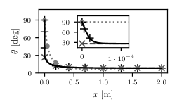
(b) Angle of major axis to flow direction.

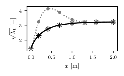
(c) Major axis length.

Figure 4: Comparison of morphology models under simple shear.

First, we consider planar two-dimensional Couette flow. This configuration is visualized in Fig. 4(a). The channel height is set to $h=2.5\cdot 10^{-5}\,\unit{}$ and the top wall moves at $U=1\,\unit{\per}$. The channel has a streamwise length of $2\,\unit{}$. The computational domain is discretized with $10{,}000$ rectangular finite elements. At the inlet, the elements have a streamwise length of $5\cdot 10^{-6}\,\unit{}$ to capture cell behavior in the entry region. The length progressively increases downstream. At the inlet, red blood cells are introduced with an initial shape of $(\lambda_{1},\lambda_{2},\lambda_{3})=(2,1,0.5)$. The angle between the flow direction and the major axis is defined as $\theta$. At the inlet, the orientation is imposed such that the major axis is orthogonal to the flow direction, i.e., $\theta_{\mathrm{in}}=90\unit{}$. The solutions for the Eulerian models 8, 10 and 15 are obtained by solving the steady state morphology problem 19.

From a Lagrangian point-of-view, planar Couette flow produces simple shear, i.e., unidirectional flow with a constant gradient perpendicular to the flow direction. Fluid strain and vorticity are of equal strength in simple shear. Their magnitude is defined by the fluid shear rate $G_{\mathrm{f}}=40{,}000\,\unit{\per}$. If we align the $x$-axis with the flow direction and the $y$-axis with the gradient direction, the flow gradients can be written as follows:

$$\bm{\mathbf{\nabla}}\bm{\mathbf{u}}=\begin{bmatrix}0&G_{\mathrm{f}}&0\\ 0&0&0\\ 0&0&0\end{bmatrix}\,.$$

For this flow field, pathlines are straight lines with $y=\mathrm{const}$. We evaluate the Lagrangian Arora model along these pathlines as described in Section 3.4. The initial condition is equivalent to the inlet boundary condition then. If we choose the pathline at the top, i.e., $y=h$ with $U=1\,\unit{\per}$, the time coordinate $t$ in the Lagrangian formulation corresponds one-to-one to the spatial coordinate $x$ in the Eulerian formulation. The solution of the Lagrangian model can thus be compared directly to the Eulerian solution.

Figure 4(b) shows the evolution of the major axis angle $\theta$. Starting from the imposed initial angle of $90^{\circ}$, the cell rapidly assumes an orientation $\theta=26.6^{\circ}$. As visualized in the inset in Fig. 4(b), the initial alignment happens within the first $0.1\,\unit{\milli}$ according to the Arora model 2. The resulting angle corresponds precisely to the steady orientation for the initial deformation and the given flow state, i.e., $\theta_{\mathrm{steady}}=26.6^{\circ}$ according to Eq. 14. Downstream, the cell remains at steady orientation $\theta_{\mathrm{steady}}$, which decreases asymptotically towards 0 with increasing cell deformation. This steady orientation represents a tank-treading state. The alignment of the major axis with the flow direction at high shear rates agrees with experimental observations [29, 12].

The Eulerian models differ in their ability to predict the initial rapid alignment. As shown in the inset, the full-order model 8 predicts the alignment perfectly. The TTM does not resolve the initial alignment, as the cell is assumed to be at steady state permanently. However, it predicts the orientation accurately after the initial alignment, i.e., $x>1\cdot 10^{-4}\,\unit{}$. In contrast, the simplified model 15 predicts a slower alignment with the steady orientation. This is due to the lower rotation rate of cells (cf. Section 2.4). The final orientation is predicted accurately by the simplified model. This is because the steady orientation represents an equilibrium between the rotational effects of strain and vorticity. The strength of these effects relative to one another is the same in the simplified model as in the full-order model. The absolute rotation rate is lower, however, causing slower transient behavior.

Figure 4(c) shows the evolution of the major axis length $\sqrt{\lambda_{1}}$. Starting from the initial deformation, the cell deforms towards a steady state deformation of $(\lambda_{1},\lambda_{2},\lambda_{3})=(10.5,0.43,0.22)$. According to Eq. 17, this corresponds to an effective shear rate of $G_{\mathrm{eff}}=40{,}000\,\unit{\per}=G_{\mathrm{f}}$. This is expected behavior, as the effective shear rate is constructed precisely to predict an equivalent simple shear flow that induces the instantaneous cell deformation at steady state. The Eulerian models agree in the prediction of this final deformation, but they differ in their prediction of transient behavior. The full-order model predicts the evolution of deformation in full agreement with the Arora model. The TTM provides an equivalent approximation. The discrepancy with respect to the initial cell orientation is limited to such small timescales that it does not affect deformation, which occurs over longer timescales. The simplified model, on the other hand, significantly overpredicts intermediate deformation. This is due to the slower alignment with the tank-treading state, which causes the cell to be more aligned with the direction of shear for longer. The steady deformation is predicted correctly due to the correct prediction of the final orientation.

Overall, this test case validates the full-order Eulerian reformulation 8, which agrees perfectly with the Lagrangian model 2. The TTM 10 only deviates slightly for the initial orientation, but agrees for the deformation. Since deformation is the primary quantity of interest, the TTM is a good approximation for the full-order model. The simplified model 15, on the other hand, deviates significantly for the transient cell deformation. This demonstrates the effects of the lower rotation rate.

4.2 Rotating shear

(a) Test case configuration

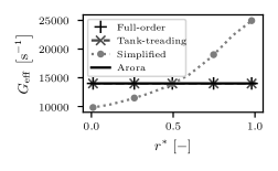
(b) Radial distribution of effective shear rate

Figure 5: Comparison of morphology models under rotating shear.

In order to explore transient cell behavior in more detail, we consider two-dimensional circular Couette flow. This test case is visualized in Fig. 5(a). We choose $R=0.701\,\unit{\centi}$, $\Delta R=0.0001\,\unit{\centi}$ and counter-rotating walls with $\omega_{\mathrm{i}}=1\,\unit{\per}$, $\omega_{\mathrm{o}}=-1\,\unit{\per}$. This system produces a nearly constant shear rate of $G_{\mathrm{f}}=14{,}021\,\unit{\per}$ across the domain. We define a non-dimensionalized radial coordinate $r^{*}=\frac{r-R}{\Delta R}\in[0,1]$. The domain is discretized with 8 elements in radial direction and 3560 elements in azimuthal direction. Due to the two-dimensional nature of the problem, the Taylor-Couette instability does not affect the flow. We simulate all Eulerian morphology models on this domain up to steady state.

The pathlines are closed circles with $r^{*}=\mathrm{const}$. Along each pathline, a cell experiences simple shear flow with a rotating direction of shear:

$$\bm{\mathbf{\nabla}}\bm{\mathbf{u}}(t)=\bm{\mathbf{R}}_{z}(\omega t)\,\begin{bmatrix}0&G_{\mathrm{f}}&0\\ 0&0&0\\ 0&0&0\end{bmatrix}\bm{\mathbf{R}}_{z}^{\mathbf{T}}(\omega t)\,,\qquad\bm{\mathbf{R}}_{z}(\varphi)=\begin{bmatrix}\cos\varphi&-\sin\varphi&0\\ \sin\varphi&\cos\varphi&0\\ 0&0&1\end{bmatrix}\,.$$

The angular frequency depends on the radius of the pathline:

$$\omega\mathopen{}\mathclose{{}\left(r^{*}}\right)=\omega_{\mathrm{i}}+\mathopen{}\mathclose{{}\left(\omega_{\mathrm{o}}-\omega_{\mathrm{i}}}\right)\mathopen{}\mathclose{{}\left(2r^{*}-1}\right)\,.$$

We evaluate the Arora model for three radii $r^{*}\in\{0,0.5,1\}$ by integrating the Lagrangian morphology model along the circular pathlines up until steady state.

In Fig. 5(b), we compare the different morphology models. With the Lagrangian Arora model, the effective shear rate $G_{\mathrm{eff}}$ is nearly constant across the range of $r^{*}$ and corresponds to fluid shear $G_{\mathrm{f}}$. As cells travel along their pathlines, they constantly realign themselves with respect to the rotating direction of shear. In the Arora model, this realignment occurs so rapidly that cells practically experience only simple shear. For simple shear, $G_{\mathrm{eff}}=G_{\mathrm{f}}$ holds in steady state, as discussed in Section 4.1.

Out of the Eulerian models, the full-order model again agrees perfectly with the Lagrangian model. The TTM agrees very well with the full-order model for these parameters. The simplified model, on the other hand, deviates significantly from the full-order model. It underpredicts cell deformation at the inner wall and overpredicts it at the outer wall. It agrees with the full-order model only at the centerline $r^{*}=0.5$. This is due to the lower rotation rate of cells in the simplified model, which causes a phase lag in their orientation as they travel along the circular pathline. At the inner wall, this phase lag causes the major axis to be less aligned with the principal axis of strain, leading to lower deformation. At the outer wall, the phase lag causes the major axis to be more aligned with the principal axis of strain, leading to higher deformation. At the centerline, cells are at rest, so they do not experience a rotating direction of shear, $\omega(r^{*}=0.5)=0$. This is equivalent to simple shear, where the simplified model agrees with the full-order model at steady state.

This test case serves as further validation for the Eulerian full-order model and the TTM, both of which agree with the Lagrangian Arora model. Furthermore, it demonstrates that the simplified model deviates from the full-order model not only in transient behavior (see Section 4.1), but also at steady state. In general, the simplified model is not suitable for any flows with non-constant gradients along its pathlines, as this requires cells to realign. This realignment incurs modeling errors due to the lower rotation rate in the simplified model. As this test case demonstrates, these errors can lead to both overprediction and underprediction of effective shear rate.

4.3 Square stirrer

In order to test the morphology models’ performance in more complex flows, we consider a two-dimensional square domain with a stirrer. The geometry and mesh are identical to those presented in previous works [34, 32]. We set a stirrer frequency of $\omega_{\mathrm{stir}}=100\,\unit{\per}$ and use the MRF approach for the rotating stirrer. The interface is visualized as a dashed line in Fig. 6(a). The computational domain is discretized with $92{,}262$ triangular elements. The initial condition is an undeformed cell. We simulate the Eulerian morphology models up to steady state.

Model	Time
Full-order	$1680\,\mathrm{s}$
Simplified	$97\,\mathrm{s}$
TTM	$8\,\mathrm{s}$

Table 1: Execution times for the square stirrer test case on 48 cores.

The models are compared with respect to computational performance in Table 1. The full-order model is the slowest, as its time step size is severely restricted by the small timescale of the cell rotation (cf. Section 4.1). This limits its applicability to simple two-dimensional flows, and it becomes prohibitively expensive for three-dimensional flows. It is thus not suited for realistic blood pump geometries. The simplified model is not affected by this issue to the same degree, as cells rotate at a slower rate. The time step limitation is thus not as severe. The TTM is more robust, since it does not resolve cell rotation explicitly. This allows for larger time steps and thus significantly faster computation.

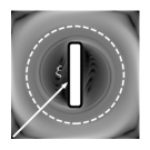
(a) Simplified model

(b) Full-order model

(c) Tank-treading model

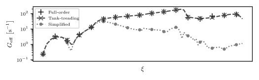
(d) Comparison between morphology models along line from lower left corner to center (see Fig. 6(a)).

Figure 6: Morphology results for square stirrer

The model predictions are compared in Fig. 6. The solution in Fig. 6(a) matches previous results using the simplified model [32]. In comparison with the full-order model in Fig. 6(b), however, it deviates significantly. In particular, it underpredicts effective shear rate close to the stirrer by two orders of magnitude. The TTM in Fig. 6(c) agrees well with the full-order model, but lacks some of the finer details of the solution in the region close to the stirrer. Finally, the three models are compared along the profile line $\xi$ in Fig. 6(d). The results for the simplified model agree qualitatively with those presented by Haßler et al. [32]. However, this agrees with the full-order model only close to the outer walls. In that region, flow velocities are lower, so cells do not have to respond to changing velocity gradients as quickly. The simplified model is thus able to predict the effective shear rate accurately. Closer to the center, cells rotate more quickly, so the modeling error due to the lower rotation rate of the simplified model becomes more significant. This causes the underprediction in that region. Conversely, the TTM agrees well with the full-order model across the whole domain.

4.4 Simple pump

The final test case involves a three-dimensional geometry. It represents a simplified version of an FDA benchmark pump [46]. For details on the geometry, we refer to Pauli et al. [6]. The domain is discretized with a total of $6{,}618{,}708$ tetrahedral elements. We simulate fluid flow through the pump with the MRF approach at a flow rate of $0.5\,\unit{\per}$, with a rotation rate of $1000\,\mathrm{rpm}$. The Eulerian morphology models 10 and 15 are solved up to steady state. The initial condition and the boundary condition at the inlet are undeformed cells. We employ the logarithmic formulation of the tank-treading morphology model (TTLM) for additional robustness.

Simulation	Time
CFD (MRF)	$20\,\mathrm{h}$
Simplified morphology	$45\,\mathrm{min}$
TTLM	$8\,\mathrm{min}$

Table 2: Execution times for the simple pump test case on 192 cores.

The execution times to obtain a steady solution for this test case are listed in Table 2. The morphology problems can be solved significantly faster than the fluid flow problem. Among the morphology models, the TTLM is faster than the simplified model by a factor of six. This is due to the lower number of degrees of freedom and the high robustness of its logarithmic formulation, allowing for larger time steps.

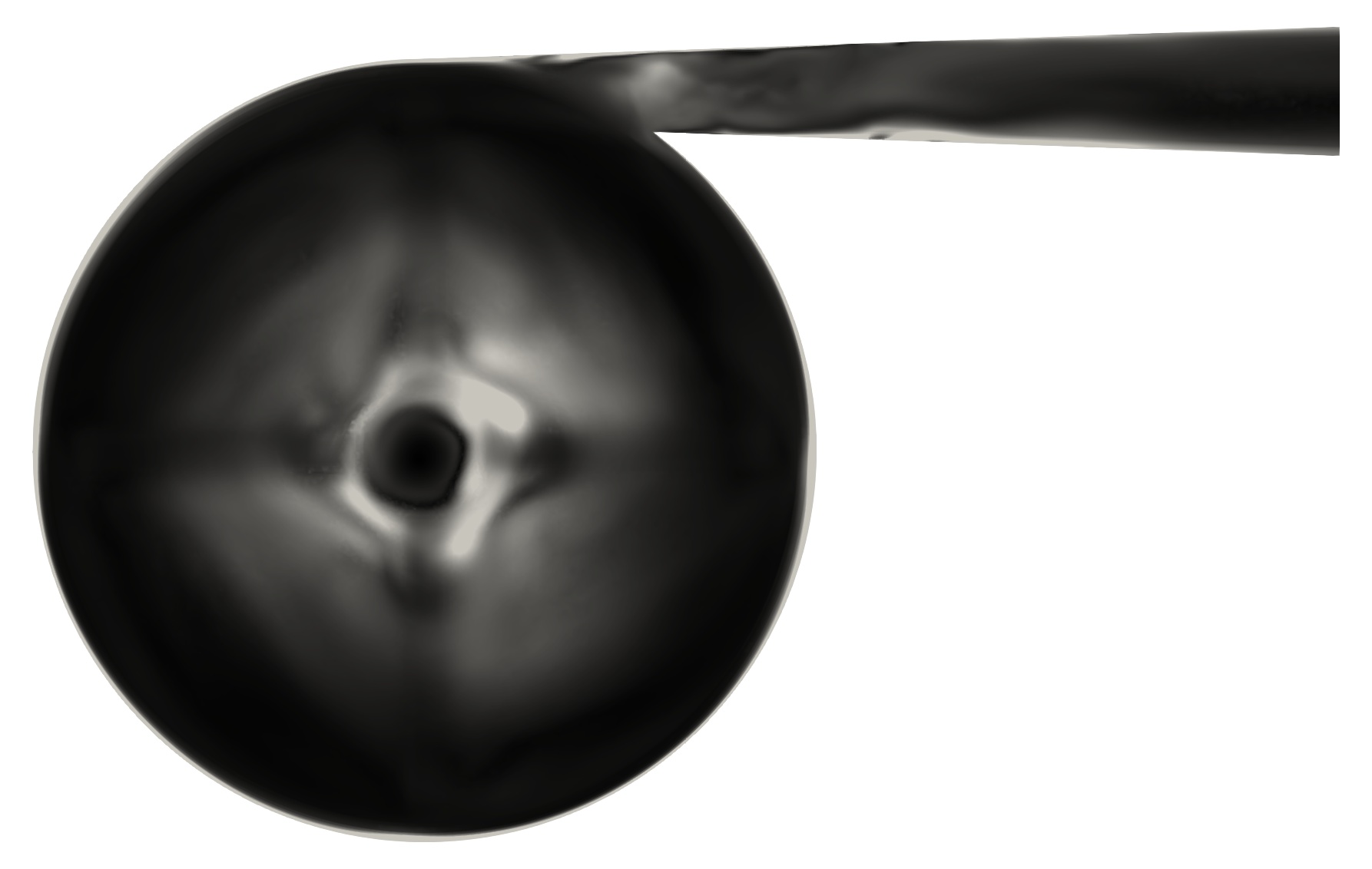
(a) Simplified model

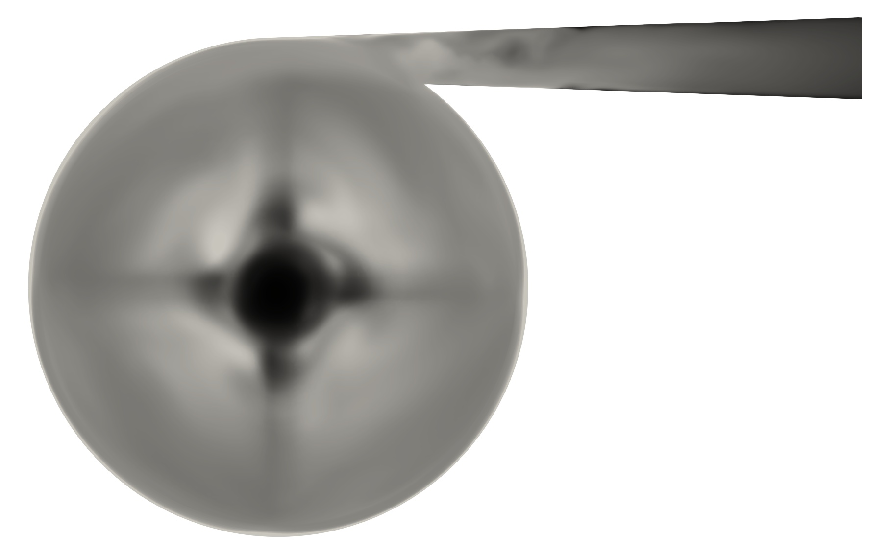
(b) Tank-treading model

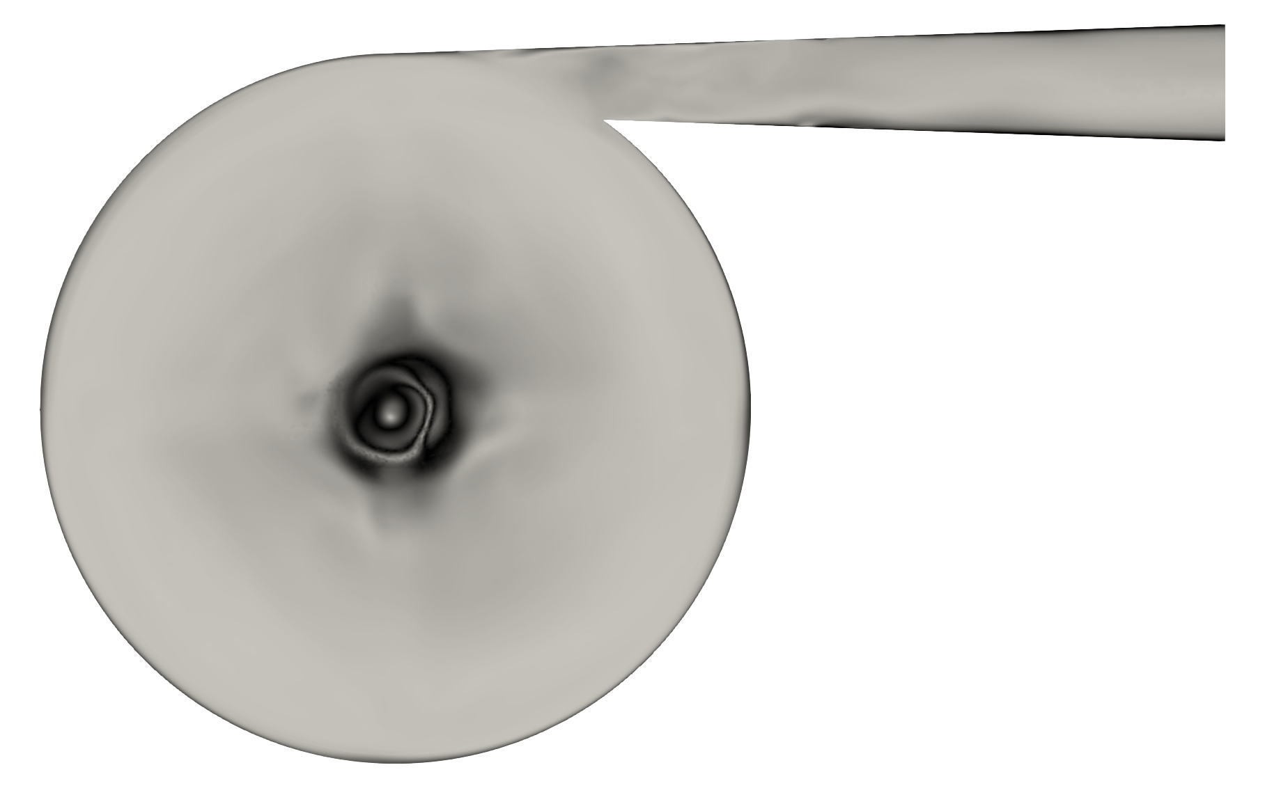
(c) Relative error of simplified model

Figure 7: Effective shear rate in simplified three-dimensional blood pump in the plane $5\,\unit{\milli}$ above the impeller blades.

Figure 7 shows the effective shear rate on a plane parallel to the impeller disk. The plane is located $0.5\,\unit{\milli}$ above the blades. The simplified model in Fig. 7(a) again underpredicts the effective shear rate severely compared to the TTLM in Fig. 7(b). The relative error $\delta=|G_{\mathrm{eff}}^{\mathrm{simpl}}-G_{\mathrm{eff}}^{\mathrm{TTLM}}|/G_{\mathrm{eff}}^{\mathrm{TTLM}}$ is shown in Fig. 7(c). Close to the outer wall and close to the inflow in the center, the two models agree. This can be explained by the same reasoning as in the square stirrer test case (cf. Section 4.3): The simplified model is able to predict the effective shear rate accurately in regions with low flow velocity, where cells do not have to respond to changing velocity gradients as quickly. Everywhere else, the simplified model underpredicts the effective shear rate by up to 98%.

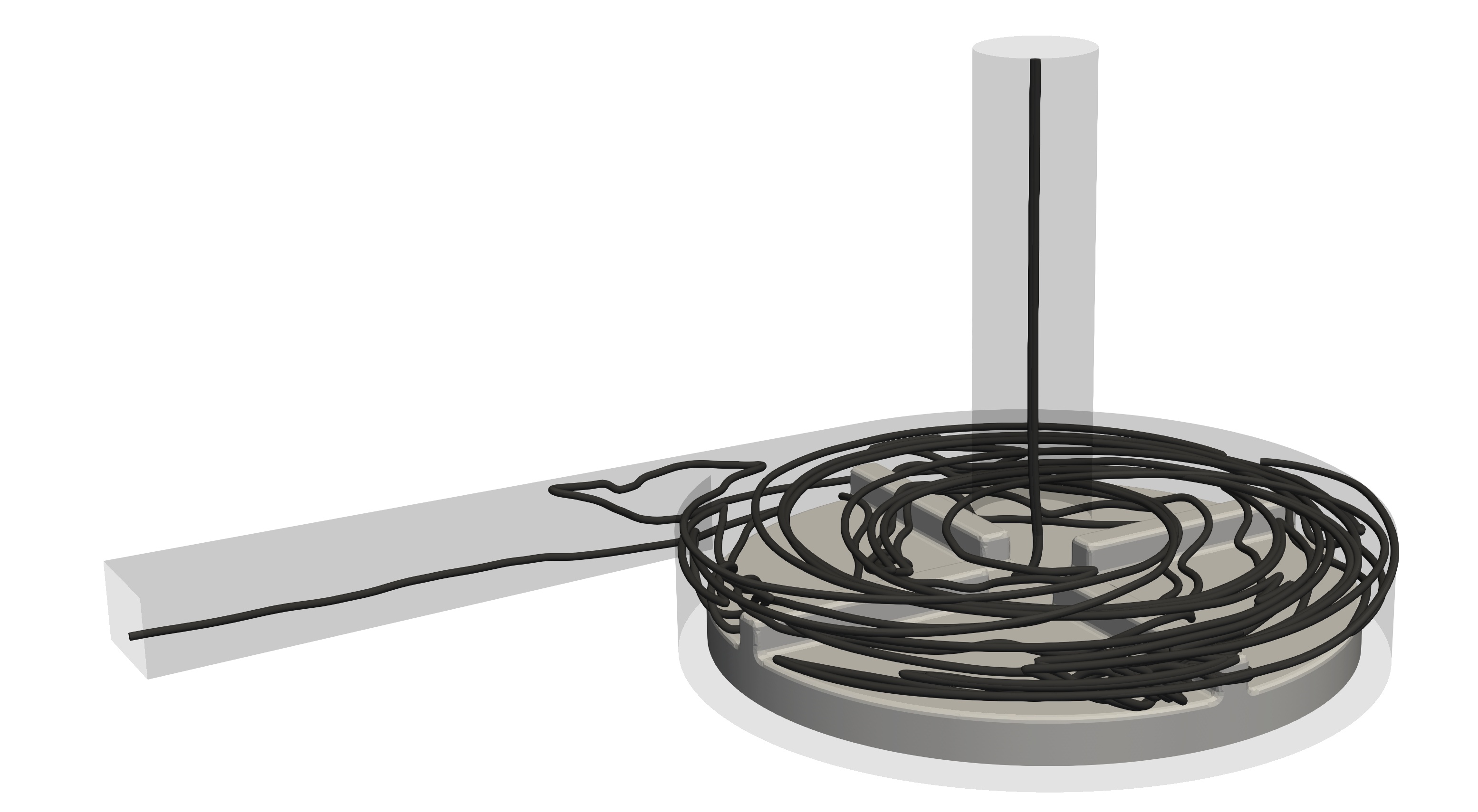
Figure 8: Selected pathlines in the simplified blood pump.

For validation, we compare the Eulerian and Lagrangian model formulations as outlined in Section 3.4. Four particular pathlines are selected and visualized in Fig. 8. The pathlines provide good coverage of the area around the impeller. However, only one of the four pathlines exits the domain through the outlet. The other pathlines terminate at walls or at the impeller. This is an artifact of the discrete nature of the velocity field and the explicit time stepping scheme used to integrate the pathlines. It presents a principal limitation of the Lagrangian approach, as it is not possible to track every cell through the whole domain, especially in complex geometries, where cells can get trapped in recirculation zones. This limitation does not apply to the Eulerian models, as they are solved on the whole domain.

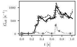
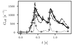
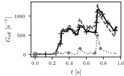
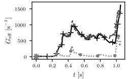
Figure 9: Eulerian and Lagrangian model formulations compared along four sample pathlines in the simple blood pump.

The model results along these particular pathlines are given in Fig. 9. The two Lagrangian solutions for Arora model and TTM are practically identical, underlining the validity of the TTM to approximate the full-order behavior. Out of the Eulerian models, the simplified model again underpredicts the effective shear rate significantly. For systems with higher rotation rates of the impeller, we expect this discrepancy to grow further, as cell rotation becomes more significant. The Eulerian formulation of the TTM agrees overall well with its Lagrangian formulation. The Eulerian formulation is more diffusive due to the finite element discretization in space. The Lagrangian formulation does not require any mesh, as its discretization is only governed by the integration step size along its pathline. This causes some local discrepancies between the solutions. However, if we integrate empirical hemolysis models along a larger set of 36 pathlines, the averaged results agree within $5\,\%$. Overall, this comparison demonstrates that the Eulerian formulation of the TTM is a valid approximation of the Lagrangian Arora model for the given application.

5 Conclusion and Outlook

Hemolysis modeling is an integral part of the design process of blood-contacting medical devices. But as of now, no standard way of modeling this phenomenon has been established. Instead, the landscape of models stretches from relatively simple Eulerian stress-based models to complex and less practical Lagrangian strain-based models. With this work, we aim to provide some middle ground by combining the unique advantages of both approaches into the Eulerian tank-treading morphology model (TTM). Compared to Eulerian stress-based models, the TTM is able to capture the viscoelastic behavior of the cell membrane by resolving cell deformation time. Compared to Lagrangian strain-based models, the TTM is computationally more efficient and does not require tracking individual cells. Compared to a previous Eulerian strain-based model [6], the TTM more accurately captures the original Lagrangian model behavior. This has been shown on the basis of a selection of benchmark flows, including simple shear, rotating shear, and two more complex rotational flows representative of VADs.

The largest limitation of the present model is its assumption of ellipsoidal cell shape. In microfluidic flows, red blood cells deform into slipper and parachute shapes [47]. Moreover, recent studies have suggested that dynamics and morphology of red blood cells are more diverse than tank-treading ellipsoids even in simple shear flow [48, 49]. We argue that the present model nevertheless provides practical predictions for two reasons. First, fully resolving small-scale cell behavior requires a more complex structural model for the cell membrane. Such models currently only allow for simulation of small ensembles of cells, many orders of magnitude away from the total number of cells in realistic configurations. They are thus not suitable for the design process of VADs. Second, scale-resolving simulations by Lanotte et al. [48] at physiological hematocrit (volume fraction of RBCs) and physiological plasma viscosities indicate that at high shear rates, elongated flattened cells with tank-treading dynamics dominate. Even though their shapes may feature irregularities compared with pure ellipsoids, orientation and characteristic deformation time should behave similarly. We thus expect the TTM to still describe the deformation of such cells adequately.

In the future, we will examine if the effects of the aforementioned morphology irregularities can be incorporated into the model phenomenologically, e.g., by adapting the model parameters $f_{1},f_{2},f_{3}$. Additionally, we are aiming to obtain experimental data for cell deformation. This will allow for further model validation and provide a basis for the calibration of the model parameters, especially in light of new results for relaxation time [50] and methods of varying the parameters [51]. Finally, we intend to apply the TTM to more realistic VAD geometries and compare its hemolysis predictions with computational and empirical reference results, e.g., for the FDA benchmark blood pump [8]. In this context, we are also planning to investigate the effects of turbulence modeling and variable hematocrit on strain-based hemolysis predictions.

Overall, we are confident that the TTM represents an excellent compromise between accuracy and practicality. It provides a solid basis for understanding the effects of bulk flow on RBCs. This will make it a valuable tool for the design process of future generations of medical devices.

Declaration of competing interest

The authors declare that they have no known competing financial interests or personal relationships that could have appeared to influence the work reported in this paper.

A On the definition of the rotation term

The left-hand side of the Arora model 2 is meant to represent a Jaumann derivative. The defining feature of a Jaumann derivative is that it is objective under rotation, i.e., in a purely rotational flow and neglecting shape recovery, it has to hold that

$$\frac{\mathrm{d}\bm{\mathbf{S}}}{\mathrm{d}t}-\mathopen{}\mathclose{{}\left[\bm{\mathbf{\Omega}},\,\bm{\mathbf{S}}}\right]=\bm{\mathbf{0}}\,.$$

Again employing the spectral decomposition 4 and noting that the eigenvalues are constant in the case of pure rotation, we find that

$$\frac{\mathrm{d}\bm{\mathbf{S}}}{\mathrm{d}t} =\frac{\mathrm{d}\bm{\mathbf{Q}}}{\mathrm{d}t}\bm{\mathbf{\Lambda}}\bm{\mathbf{Q}}^{\mathbf{T}}+\bm{\mathbf{Q}}\bm{\mathbf{\Lambda}}\frac{\mathrm{d}\bm{\mathbf{Q}}^{\mathbf{T}}}{\mathrm{d}t}\,,$$

$$\mathopen{}\mathclose{{}\left[\bm{\mathbf{\Omega}},\,\bm{\mathbf{S}}}\right] =\bm{\mathbf{\Omega}}\bm{\mathbf{Q}}\bm{\mathbf{\Lambda}}\bm{\mathbf{Q}}^{\mathbf{T}}-\bm{\mathbf{Q}}\bm{\mathbf{\Lambda}}\bm{\mathbf{Q}}^{\mathbf{T}}\bm{\mathbf{\Omega}}\,.$$

Thus, objectivity is ensured if

$$\frac{\mathrm{d}\bm{\mathbf{Q}}}{\mathrm{d}t}=\bm{\mathbf{\Omega}}\bm{\mathbf{Q}}\qquad\text{and}\qquad\frac{\mathrm{d}\bm{\mathbf{Q}}^{\mathbf{T}}}{\mathrm{d}t}=\bm{\mathbf{Q}}^{\mathbf{T}}\bm{\mathbf{\Omega}}\,.$$

These equations are only satisfied by the definition 1. In contrast, Arora [5] employed the definition

$$\tilde{\bm{\mathbf{\Omega}}}=-\frac{\mathrm{d}\bm{\mathbf{Q}}^{\mathbf{T}}}{\mathrm{d}t}\bm{\mathbf{Q}}=\bm{\mathbf{Q}}^{\mathbf{T}}\frac{\mathrm{d}\bm{\mathbf{Q}}}{\mathrm{d}t}=\bm{\mathbf{Q}}^{\mathbf{T}}\frac{\mathrm{d}\bm{\mathbf{Q}}}{\mathrm{d}t}\bm{\mathbf{Q}}\bm{\mathbf{Q}}^{\mathbf{T}}=\bm{\mathbf{Q}}^{\mathbf{T}}\bm{\mathbf{\Omega}}\bm{\mathbf{Q}}\,,$$

which corresponds to a change of basis to the coordinate system of the cell. In tensor notation, the two definitions are equivalent.

References

- [1] T. Vos, S. S. Lim, et al., Global Burden of 369 Diseases and Injuries in 204 Countries and Territories, 1990–2019: A Systematic Analysis for the Global Burden of Disease Study 2019, The Lancet 396 (10258) (2020) 1204–1222.
- [2] G. Heuser, R. Opitz, A Couette Viscometer for Short Time Shearing of Blood, Biorheology 17 (1980) 17–24.
- [3] M. Giersiepen, L.J. Wurzinger, R. Opitz, H. Reul, Estimation of Shear Stress-Related Blood Damage in Heart Valve Prostheses—In Vitro Comparison of 25 Aortic Valves, International Journal of Artificial Organs 13 (5) (1990) 300–306.
- [4] C. Bludszuweit, Model for a General Mechanical Blood Damage Prediction, Artificial Organs 19 (7) (1995) 583–589.
- [5] D. Arora, M. Behr, M. Pasquali, A Tensor-Based Measure for Estimating Blood Damage, Artificial Organs 28 (11) (2004) 1002–1015.
- [6] L. Pauli, J. Nam, M. Pasquali, M. Behr, Transient Stress-Based and Strain-Based Hemolysis Estimation in a Simplified Blood Pump, International Journal for Numerical Methods in Biomedical Engineering 29 (2013) 1148–1160.
- [7] M. M. Faghih, M. K. Sharp, Modeling and Prediction of Flow-Induced Hemolysis: A Review, Biomechanics and Modeling in Mechanobiology 18 (2019) 845–881.
- [8] S. V. Ponnaluri, P. Hariharan, L. H. Herbertson, K. B. Manning, R. A. Malinauskas, B. A. Craven, Results of the Interlaboratory Computational Fluid Dynamics Study of the FDA Benchmark Blood Pump, Annals of Biomedical Engineering 51 (1) (2023) 253–269.
- [9] J. N. Katz, B. C. Jensen, P. P. Chang, S. L. Myers, F. D. Pagani, J. K. Kirklin, A Multicenter Analysis of Clinical Hemolysis in Patients Supported with Durable, Long-Term Left Ventricular Assist Device Therapy, The Journal of Heart and Lung Transplantation 34 (5) (2015) 701–709.
- [10] M. Puig-de-Morales-Marinkovic, K. T. Turner, J. P. Butler, J. J. Fredberg, S. Suresh, Viscoelasticity of the Human Red Blood Cell, American Journal of Physiology-Cell Physiology 293 (2) (2007) C597–C605.
- [11] T. Zhang, M. E. Taskin, H.-B. Fang, A. Pampori, R. Jarvik, B. P. Griffith, Z. J. Wu, Study of Flow-Induced Hemolysis Using Novel Couette-Type Blood-Shearing Devices, Artificial Organs 35 (12) (2011) 1180–1186.
- [12] H. L. Goldsmith, J. Marlow, F. C. MacIntosh, Flow Behaviour of Erythrocytes – I. Rotation and Deformation in Dilute Suspensions, Proceedings of the Royal Society of London. Series B. Biological Sciences 182 (1068) (1972) 351–384.
- [13] L. A. Down, D. V. Papavassiliou, E. A. O’Rear, Significance of Extensional Stresses to Red Blood Cell Lysis in a Shearing Flow, Annals of Biomedical Engineering 39 (6) (2011) 1632–1642.
- [14] M. M. Faghih, M. K. Sharp, Deformation of Human Red Blood Cells in Extensional Flow through a Hyperbolic Contraction, Biomechanics and Modeling in Mechanobiology 19 (1) (2020) 251–261.
- [15] Y. Chen, M. K. Sharp, A Strain-Based Flow-Induced Hemolysis Prediction Model Calibrated by In Vitro Erythrocyte Deformation Measurements, Artificial Organs 35 (2) (2011) 145–156.
- [16] Y. Chen, T. L. Kent, M. K. Sharp, Testing of Models of Flow-Induced Hemolysis in Blood Flow Through Hypodermic Needles, Artificial Organs 37 (3) (2013) 256–266.
- [17] H. Yu, S. Engel, G. Janiga, D. Thévenin, A Review of Hemolysis Prediction Models for Computational Fluid Dynamics, Artificial Organs 41 (7) (2017) 603–621.
- [18] G. Arwatz, A. J. Smits, A Viscoelastic Model of Shear-Induced Hemolysis in Laminar Flow, Biorheology 50 (1-2) (2013) 45–55.
- [19] H. M. Ezzeldin, M. D. de Tullio, M. Vanella, S. D. Solares, E. Balaras, A Strain-Based Model for Mechanical Hemolysis Based on a Coarse-Grained Red Blood Cell Model, Annals of Biomedical Engineering 43 (6) (2015) 1398–1409.
- [20] S. Sohrabi, Y. Liu, A Cellular Model of Shear-Induced Hemolysis, Artificial Organs 41 (9) (2017) E80–E91.
- [21] C. Porcaro, M. Saeedipour, Hemolysis Prediction in Bio-Microfluidic Applications Using Resolved CFD-DEM Simulations, Computer Methods and Programs in Biomedicine 231 (2023) 107400.
- [22] D. A. Fedosov, B. Caswell, G. E. Karniadakis, A Multiscale Red Blood Cell Model with Accurate Mechanics, Rheology, and Dynamics, Biophysical Journal 98 (10) (2010) 2215–2225.
- [23] T. Klöppel, W. A. Wall, A Novel Two-Layer, Coupled Finite Element Approach for Modeling the Nonlinear Elastic and Viscoelastic Behavior of Human Erythrocytes, Biomechanics and Modeling in Mechanobiology 10 (4) (2011) 445–459.
- [24] S. Mendez, E. Gibaud, F. Nicoud, An Unstructured Solver for Simulations of Deformable Particles in Flows at Arbitrary Reynolds Numbers, Journal of Computational Physics 256 (2014) 465–483.
- [25] G. Závodszky, B. van Rooij, V. Azizi, A. Hoekstra, Cellular Level In-Silico Modeling of Blood Rheology with an Improved Material Model for Red Blood Cells, Frontiers in Physiology 8 (2017).
- [26] C. Kotsalos, J. Latt, B. Chopard, Bridging the Computational Gap between Mesoscopic and Continuum Modeling of Red Blood Cells for Fully Resolved Blood Flow, Journal of Computational Physics 398 (2019) 108905.
- [27] F. Guglietta, M. Behr, L. Biferale, G. Falcucci, M. Sbragaglia, On the Effects of Membrane Viscosity on Transient Red Blood Cell Dynamics, Soft Matter 16 (2020) 6191–6205.
- [28] G. Foster, Third-Generation Ventricular Assist Devices, in: S. D. Gregory, M. C. Stevens, J. F. Fraser (Eds.), Mechanical Circulatory and Respiratory Support, Academic Press, 2018, pp. 151–186.
- [29] H. Schmid-Schönbein, R. Wells, Fluid Drop-Like Transition of Erythrocytes under Shear, Science 165 (3890) (1969) 288–291.
- [30] T.M. Fischer, M. Stöhr-Liesen, H. Schmid-Schönbein, The Red Cell as a Fluid Droplet: Tank Tread-Like Motion of the Human Erythrocyte Membrane in Shear Flow, Science 202 (4370) (1978) 894–896.
- [31] P.L. Maffettone, M. Minale, Equation of Change for Ellipsoidal Drops in Viscous Flow, Journal of Non-Newtonian Fluid Mechanics 78 (1998) 227–241.
- [32] S. Haßler, L. Pauli, M. Behr, The Variational Multiscale Formulation for the Fully-Implicit Log-Morphology Equation as a Tensor-Based Blood Damage Model, International Journal for Numerical Methods in Biomedical Engineering 35 (12) (2019) e3262–1–e3262–19.
- [33] L. Goubergrits, Numerical Modeling of Blood Damage: Current Status, Challenges and Future Prospects, Expert Review of Medical Devices 3 (5) (2006) 527–531.
- [34] L. Pauli, Stabilized Finite Element Methods for Computational Design of Blood-Handling Devices, Ph.D. thesis, RWTH Aachen University, Aachen, Germany (2016).
- [35] L. Pauli, M. Behr, On Stabilized Space-Time FEM for Anisotropic Meshes: Incompressible Navier-Stokes Equations and Applications to Blood Flow in Medical Devices, International Journal for Numerical Methods in Fluids 85 (3) (2017) 189–209.
- [36] L. Pauli, J. Both, M. Behr, Stabilized Finite Element Method for Flows with Multiple Reference Frames, International Journal for Numerical Methods in Fluids 78 (11) (2015) 657–669.
- [37] T.J.R. Hughes, M. Mallet, A New Finite Element Formulation for Computational Fluid Dynamics: III. The Generalized Streamline Operator for Multidimensional Advective-Diffusive Systems, Computer Methods in Applied Mechanics and Engineering 58 (1986) 305–328.
- [38] Y. Bazilevs, V. M. Calo, T. E. Tezduyar, T. J. R. Hughes, YZ Discontinuity Capturing for Advection-Dominated Processes with Application to Arterial Drug Delivery, International Journal for Numerical Methods in Fluids 54 (6-8) (2007) 593–608.
- [39] D. Hilger, N. Hosters, F. Key, S. Elgeti, M. Behr, A Novel Approach to Fluid-Structure Interaction Simulations Involving Large Translation and Contact, in: H. Van Brummelen, C. Vuik, M. Möller, C. Verhoosel, B. Simeon, B. Jüttler (Eds.), Isogeometric Analysis and Applications 2018, Vol. 133, Springer International Publishing, Cham, 2021, pp. 39–56.
- [40] J. Helmig, F. Key, M. Behr, S. Elgeti, Combining Boundary-Conforming Finite Element Meshes on Moving Domains Using a Sliding Mesh Approach, International Journal for Numerical Methods in Fluids 93 (4) (2021) 1053–1073.
- [41] F. A. González, S. Elgeti, M. Behr, The Surface-Reconstruction Virtual-Region Mesh Update Method for Problems with Topology Changes, International Journal for Numerical Methods in Engineering 124 (9) (2023) 2050–2067.
- [42] F. Key, L. Pauli, S. Elgeti, The Virtual Ring Shear-Slip Mesh Update Method, Computers & Fluids 172 (2018) 352–361.
- [43] F. Key, M. von Danwitz, F. Ballarin, G. Rozza, Model Order Reduction for Deforming Domain Problems in a Time-Continuous Space-Time Setting, International Journal for Numerical Methods in Engineering 124 (23) (2023) 5125–5150.
- [44] F. Key, F. Ballarin, S. Eusterholz, S. Elgeti, G. Rozza, Reduced Flow Model for Plastics Melt Inside an Extrusion Die, Proceedings in Applied Mathematics and Mechanics 21 (1) (2021) e202100071.
- [45] J. S. Hesthaven, G. Rozza, B. Stamm, Certified Reduced Basis Methods for Parametrized Partial Differential Equations, SpringerBriefs in Mathematics, Springer International Publishing, 2015.
- [46] S. F. C. Stewart, E. G. Paterson, G. W. Burgreen, P. Hariharan, M. Giarra, V. Reddy, S. W. Day, K. B. Manning, S. Deutsch, M. R. Berman, M. R. Myers, R. A. Malinauskas, Assessment of CFD Performance in Simulations of an Idealized Medical Device: Results of FDA’s First Computational Interlaboratory Study, Cardiovascular Engineering and Technology 3 (2) (2012) 139–160.
- [47] D. A. Fedosov, M. Peltomäki, G. Gompper, Deformation and Dynamics of Red Blood Cells in Flow through Cylindrical Microchannels, Soft Matter 10 (24) (2014) 4258–4267.
- [48] L. Lanotte, J. Mauer, S. Mendez, D. A. Fedosov, J.-M. Fromental, V. Claveria, F. Nicoud, G. Gompper, M. Abkarian, Red Cells’ Dynamic Morphologies Govern Blood Shear Thinning under Microcirculatory Flow Conditions, Proceedings of the National Academy of Sciences of the United States of America 113 (47) (2016) 13289–13294.
- [49] J. Mauer, S. Mendez, L. Lanotte, F. Nicoud, M. Abkarian, G. Gompper, D. A. Fedosov, Flow-Induced Transitions of Red Blood Cell Shapes under Shear, Physical Review Letters 121 (11) (2018) 118103.
- [50] F. Guglietta, M. Behr, G. Falcucci, M. Sbragaglia, Loading and Relaxation Dynamics of a Red Blood Cell, Soft Matter 17 (2021) 5978–5990.
- [51] D. Taglienti, F. Guglietta, M. Sbragaglia, Reduced Model for Droplet Dynamics in Shear Flows at Finite Capillary Numbers, Physical Review Fluids 8 (1) (2023) 013603.