Optimal design of equilibrium solutions of the Vlasov-Poisson system by an external electric field

Abstract

A new optimization framework to design steady equilibrium solutions of the Vlasov-Poisson system by means of external electric fields is presented. This optimization framework requires the minimization of an ensemble functional with Tikhonov regularization of the control field under the differential constraint of a nonlinear elliptic equation that models equilibrium solutions of the Vlasov-Poisson system. Existence of optimal control fields and their characterization as solutions to first-order optimality conditions are discussed. Numerical approximations and optimization schemes are developed to validate the proposed framework.

Keywords:

Optimal control theory, nonlinear Poisson–Boltzmann equations, Vlasov equation.

MSC:

49J15, 49J20, 49K15, 49M05, 65K10.

1 Introduction

The need to confine and manipulate plasma appears in a multitude of applications ranging from plasma cooling [1] to satellite electric propulsion [2] and energy production in fusion reactors [3]. In particular, in many of these applications, there is the need to determine steady equilibrium configurations having specific properties useful for the given application. For this reason, many different strategies have been proposed and analyzed [4, 5, 6].

We would like to contribute to this field of research with the formulation of a novel optimization framework for optimal design of equilibrium configurations that we exemplify considering a Vlasov-Poisson system subject to an external electric control field. The main novelties of our approach are: 1) The introduction of an ensemble objective functional with a first-order Tikhonov regularization of the external control field sought; 2) The choice of the differential constraint given by a nonlinear elliptic equation that models the equilibrium solutions of the Vlasov-Poisson system with a given external field; 3) The complete theoretical analysis of the resulting optimization problem; 4) The numerical validation of the proposed optimal design procedure.

The Vlasov-Poisson system governs the transport of a particle distribution function $f$ under the action of a self-consistent force whose potential is modelled by a Poisson equation corresponding to electrostatic forces between charged particles with the same sign. Existence and uniqueness of classical solutions has been proved for dimensions $n\leq 3$ under mild assumptions on the initial data in [7, 8, 9], and weak solutions are discussed in [10, 11]. In many situations, the Vlasov-Poisson system represents an accurate alternative to the Boltzmann description of gases of charged particles whose Coulomb interaction cannot be considered to be of short-range type. We choose the Vlasov-Poisson system since it is a valid model in describing various phenomena in plasma physics and therefore it is a representative for the class of problems considered in our work.

Specifically, we consider steady equilibria solutions of the Vlasov-Poisson system that are characterized by the solution to the nonlinear elliptic Poisson-Boltzmann equation, see [12, 13, 14, 15], including the presence of an external electric control field. Our purpose is to design this control field such that the corresponding steady equilibrium distribution concentrates on some selected regions of the computational domain.

For this purpose, we formulate a constrained optimization problem, whose differential constraint is the nonlinear Poisson-Boltzmann equation with the external control field to be optimized by minimizing a regularized ensemble objective functional. Our choice of an ensemble functional is dictated by the statistical nature of the underlying Vlasov-Poisson system and differs considerably from $L^{2}$ error tracking functionals as the one considered in, e.g., [5, 6], where a desired distribution profile must be provided that could be unattainable for the given physical setting. In fact, our ensemble functional corresponds to a statistical expected value functional of a valley-potential in which we wish to concentrate the particle density. This class of functionals was introduced in [16] and recently applied and analyzed in [17, 18, 19]. Moreover, in order to guarantee well posedness of our optimization problem and the appropriate regularity of the resulting optimal control field, our objective functional includes a first-order Tikhonov regularization term; see, e.g., [20] for a discussion on Tikhonov regularization of different orders.

In this work, we theoretically investigate the proposed optimization problem proving existence of optimal control fields. Further, we discuss the characterization of these solutions by first-order optimality conditions that result in an optimality system consisting of the Poisson-Boltzmann model, its optimization adjoint, and an optimality gradient condition. In this way, we are able to identify the gradient of the objective functional subject to the differential constraint, which is required in order to construct a numerical optimization procedure aiming at solving the optimality system. For this purpose, since the control field is sought in the Sobolev space of $H^{1}$ functions, we discuss the construction of the reduced gradient in this Hilbert space.

In Section 2, we illustrate the Vlasov-Poisson system that models the evolution of the charged particles distribution function in phase space. Further, we derive the nonlinear Poisson-Boltzmann elliptic equation for steady equilibrium distributions corresponding to a given external electric field. In Section 3, we identify this electric field as our control function and formulate our optimal external electric field problem. For this purpose, we introduce an ensemble objective functional, including a $H^{1}$ Tikhonov regularization term, which has to be minimized subject to the differential constraint given by the nonlinear elliptic equation. In this section, the regularity of the control-to-state map is discussed in detail, and existence of optimal solutions is proved. In Section 4, we discuss the characterization of optimal control fields by first-order optimality conditions. In particular, we identify the reduced gradient that is used in our iterative solution procedure.

In Section 5, we discuss the numerical implementation of our optimization framework that requires the numerical approximation of the Poisson-Boltzmann equation and of its optimization adjoint, and the assembling of the $H^{1}$ gradient that is used in a gradient-based iterative solution procedure. Further, we illustrate a nonlinear conjugate gradient algorithm with $H^{1}$ gradient to compute the optimal control fields. In Section 6, we report results of numerical experiments that demonstrate the ability of our optimization framework to manipulate the steady equilibrium plasma configuration by an external electric field. A conclusion Section completes this work.

2 The Vlasov-Poisson system and
its equilibrium solutions

The Vlasov equation [21] is a partial differential equation that models the evolution in the phase space of the distribution function of a plasma of charged interacting particles. In the zero-magnetic field limit, the Vlasov equation for charged particles subject to a given external electric field reads

$$\partial_{t}f+v\cdot\nabla_{x}f+\big{(}E(x,t)+E_{0}(x)\big{)}\cdot\nabla_{v}f=0,$$ (2.1)

where $f=f(x,v,t)$ denotes the distribution function, with $x$, $v$ and $t$ respectively being position, velocity and time, $E=E(x,t)$ represents the self-consistent (internal) electric field generated by the particles, and $E_{0}=E_{0}(x)$ is a stationary external electric field.

We are dealing with the case of positively charged particles, for which the self-consistent field is defined as the solution to the following Poisson problem

$$\operatorname*{div}E(x,t)=\rho(x,t),\qquad\rho(x,t)=\int_{{\mathbb{R}}^{n}}f(x,v,t)\,dv,$$ (2.2)

for any fixed time $t\geq 0$; we denote with $\operatorname*{div}$ the divergence in $x$, while $\rho$ is the spatial particle density, and $n$ is the spatial dimension.

For both electric fields $E$ and $E_{0}$, we assume that there exist differentiable potentials $U$ and $u$, respectively, such that it holds

$$E(x,t)=-\nabla_{x}U(x,t),\qquad E_{0}(x)=-\nabla_{x}u(x).$$ (2.3)

We also assume that the particles of the plasma are spatially localized within a bounded and convex set $\Omega\subset{\mathbb{R}}^{n}$ with smooth boundary, and the mean velocity of this system of particles is zero.

It is well known [12, 14, 22] that these conditions are sufficient for proving existence of stationary Maxwellian solutions to (2.1) with the following structure

$$f_{s}(x,v)=\frac{1}{(2\pi T)^{n/2}}\,\rho(x)\,e^{-\frac{|v|^{2}}{2T}},$$ (2.4)

where $T>0$ denotes the constant temperature of the plasma.

Notice that (2.4) is completely specified by $\rho$ that satisfies the following system

$$\nabla_{x}\rho=\frac{1}{T}\,(E+E_{0})\,\rho,\qquad\operatorname*{div}E=\rho\,;$$

see (2.1) and (2.2). Thus, using (2.3), it appears sufficient to find $\rho$ that satisfies the following equations

$$\nabla_{x}\log\rho=-\frac{1}{T}\,(\nabla_{x}U+\nabla_{x}u),\qquad-\Delta U=\rho,$$ (2.5)

where $\Delta$ represents the Laplacian operator in $x$. With the first equation in (2.5), we arrive at a formula for $\rho$ as a function of the potentials, which including $L^{1}$ normalization, is given by

$$\rho(x)=\frac{e^{-(U(x)+u(x))/T}}{\int_{\Omega}e^{-(U(x)+u(x))/T}\,dx}.$$ (2.6)

Clearly, in the stationary case the dependence on time of $E$, respectively $U$, is also dropped. We remark that, with the chosen normalization, we can interpret $\rho$ as a probability density function.

With the second equation in (2.5), and (2.6), we obtain the nonlinear Poisson-Boltzmann equation for $U$, given $u$, as follows:

$$-\Delta U(x)=\frac{e^{-(U(x)+u(x))/T}}{\int_{\Omega}e^{-(U(x)+u(x))/T}\,dx}.$$ (2.7)

It could be convenient to introduce $\rho_{0}(x)=e^{-u(x)/T}$, and with this setting, we get

$$-\Delta U(x)=\frac{\rho_{0}(x)\,e^{-U(x)/T}}{\int_{\Omega}\rho_{0}(x)\,e^{-U(x)/T}\,dx}.$$ (2.8)

Further, we can take $\Omega$ sufficiently large so that $U=0$ can be assumed on $\partial\Omega$. For simplicity, in the following we set $T=1$.

The existence and uniqueness of solutions to (2.7) with homogeneous Dirichlet boundary conditions has been studied by variational methods in [14, 15, 22]. In the following, for the sake of completeness, we give a sketch of the proof by means of an alternative approach.

Let us start introducing $u_{0}\equiv 0$, and $U_{k}$, $k=1,2,\dots$, in such a way that

$$-\Delta U_{k}(x)=\frac{e^{-(U_{k-1}(x)+u(x))/T}}{\int_{\Omega}e^{-(U_{k-1}(x)+u(x))/T}\,dx}=:f_{k}(x).$$

The existence of these functions is assured by results on linear second order elliptic equations [23]; moreover, we have $||f_{k}||_{L^{1}(\Omega)}=1$, $k\in\mathbb{N}$. Note that, since $L^{2}(\Omega)$ is continuously embedded into $L^{1}(\Omega)$, it follows that the sequence $\{f_{k}\}_{k=1}^{\infty}$ is bounded in $L^{2}(\Omega)$. Regularity results on linear second-order elliptic equations [23] imply that there exists a constant $C>0$ such that $||U_{k}||_{H^{2}(\Omega)}\leq C$, $k\in\mathbb{N}$. Therefore there exists a function $U\in H^{2}(\Omega)$ such that $U_{k}\rightharpoonup U$ in $H^{2}(\Omega)$, after extraction of a subsequence, if necessary. Passing to the limit for $k\rightarrow+\infty$, it is possible to prove that $U$ solves the equation under consideration.

Concerning the uniqueness of solutions to our elliptic problem, we exploit the same technique used in [15] for proving the uniqueness in the case without an external field. By contradiction let $U_{1}\neq U_{2}\in C^{2}(\Omega)\cap C(\overline{\Omega})$ two solutions of equation (2.7), and

$$I_{i}:=\int_{\Omega}\exp{(-u-U_{i})}\,dx,\,\,i=1,2.$$

Notice that $-\Delta U_{i}>0,\,\,i=1,2$, since $\frac{\exp{(-u-U_{i})}}{I_{i}}>0,\,\,i=1,2$, therefore $U_{1}$ and $U_{2}$ are concave. Suppose that $I_{1}>I_{2}$ and $\max_{x\in\Omega}\Big{(}U_{1}-U_{1}\Big{)}>0$, and let $\overline{x}\in\Omega$ be a point of maximum for $U_{1}-U_{2}$, then $-\Delta\Big{(}U_{1}-U_{2}\Big{)}(\overline{x})\geq 0.$ Being $I_{1}>I_{2},$ we have

$$\Bigg{(}-\frac{I_{1}}{I_{2}}\Delta U_{1}+\Delta U_{2}\Bigg{)}(\overline{x})\geq\Bigg{(}-\Delta U_{1}+\Delta U_{2}\Bigg{)}(\overline{x})\geq 0.$$

On the other hand

$$\Bigg{(}-I_{1}\Delta U_{1}+I_{2}\Delta U_{2}\Bigg{)}(\overline{x})=\exp{(-u(\overline{x}))}\Bigg{[}\exp{(-U_{1}(\overline{x}))}-\exp{(-U_{2}(\overline{x}))}\Bigg{]}<0,$$

which is in contradiction with the previous inequality.
We have shown that if $I_{1}>I_{2}$, then $U_{1}(x)\leq U_{2}(x),\,\,\forall x\in\Omega.$ By the same reasoning, one can prove that if $I_{1}=I_{2}$, then $U_{1}(x)=U_{2}(x),\,\,\forall x\in\Omega$, which results in a contradiction.

Now, without loss of generality, let us suppose that $I_{1}>I_{2}$. Then, as shown, we have $U_{1}(x)\leq U_{2}(x)$. Suppose that $\min_{x\in\Omega}\Big{(}U_{1}-U_{2}\Big{)}<0$ and let $\overline{x}\in\Omega$ be a point of minimum, we have

$$-\Delta\Big{(}U_{1}-U_{2}\Big{)}(\overline{x})\leq 0.$$ (2.9)

We have also

$$-\Delta\Big{(}U_{1}-U_{2}\Big{)}(\overline{x})=\exp{(-u(\overline{x}))}\Bigg{[}\frac{\exp{(-U_{1}(\overline{x}))}}{I_{1}}-\frac{\exp{(-U_{2}(\overline{x}))}}{I_{2}}\Bigg{]}.$$ (2.10)

Since

$$\exp{(-u(x)-U_{1}(x)+U_{1}(\overline{x}))}\leq\exp{(-u(x)-U_{2}(x)+U_{2}(\overline{x}))},$$

the second factor in the right-hand side of (2.10) must satisfy the following inequality

$$\frac{\exp{(-U_{1}(\overline{x}))}}{I_{1}}-\frac{\exp{(-U_{2}(\overline{x}))}}{I_{2}}=\frac{1}{\int_{\Omega}\exp{(-u(x)-U_{1}(x)+U_{1}(\overline{x}))}\,dx}$$

$$- \frac{1}{\int_{\Omega}\exp{(-u(x)-U_{2}(x)+U_{2}(\overline{x}))}\,dx}\geq 0.$$

There are two possibilities.

• The equality holds, then $(U_{2}-U_{1})(x)=(U_{2}-U_{1})(\overline{x})$, $\forall x\in\overline{\Omega}$, and we have a contradiction since $(U_{2}-U_{1})(x)=0$ on $x\in\partial\Omega.$

• The strict inequality holds, and we again have a contradiction with (2.9).

This concludes the proof.

3 Optimal control of equilibrium distributions

Our governing model is the nonlinear elliptic equation (2.7) with homogeneous Dirichlet boundary conditions. The solution of this boundary-value problem for a given $u$ belonging to a suitable space $D(\Omega)$ to be specified below, defines the map

$$u\mapsto U.$$

In turn, the function above and (2.6) define the composed map

$$u\mapsto\rho=\Phi(U,u),$$

where

$$\Phi(U,u):=\frac{e^{-(U+u)}}{\int_{\Omega}e^{-(U(x)+u(x))}\,dx}.$$ (3.1)

Our purpose is to formulate optimal control problems that allow us to construct external potential fields $u$, acting on the plasma, such that a distribution function with some desired properties is obtained. For this reason we consider an objective functional belonging to the class of ensemble cost functionals; see, e.g., [17, 18, 19] and references therein. Specifically, we focus on the following objective functional

$$J(\rho,u)=\int_{\Omega}V(x)\,\rho(x)\,dx+\frac{\alpha}{2}\,\|u\|^{2}_{H^{1}(\Omega)}.$$ (3.2)

In (3.2), we have a weight $\alpha>0$ that multiplies the $H^{1}$ cost of the potential $u$ as in [24]. This choice is motivated by the fact that a potential in $H^{1}(\Omega)$ is sought. The first term in (3.2) models the requirement that, by minimization, the density $\rho$ concentrates along the bottom of the ‘valley’ function $V$, which is assumed to be measurable and bounded throughout the manuscript. In particular, if we choose

$$V(x)=-A\,\exp\left(-\frac{|x-x_{0}|^{2}}{2\,a^{2}}\right),\qquad A>0,\quad a>0.$$

the bottom is at $x=x_{0}$. With the same reasoning, it is also possible to aim at designing a multimodal $\rho$, or one distributed on a ring, etc.

Another possible objective functional could be given by

$$J(\rho,u)=\frac{1}{2}G(\rho,\rho_{d})+\frac{\alpha}{2}\,\|u\|^{2}_{H^{1}(\Omega)},$$ (3.3)

where $G(\rho,\rho_{d})$ denotes an appropriate distance between $\rho$ and a desired $L^{1}$-normalized target distribution $\rho_{d}$. In particular, one could focus on the Kullback-Leibler (KL) divergence given by [25]

$$G(\rho,\,\rho_{d}):=\int_{\Omega}\rho(x)\,\log(\rho(x)/\rho_{d}(x))\,dx.$$ (3.4)

The KL divergence is a well-known type of statistical distance that measures how one probability distribution is different from a second reference one. We remark that our framework can be extended with only minor modification to accommodate the KL functional given above.

Now, we focus on the case with (3.2) and formulate our class of optimal control problems:

$$\min J(\rho,u)$$

$$\mbox{ s.t.}\quad\rho =\Phi(U,u),$$

$$-\Delta U =\Phi(U,u)\qquad\mbox{ in }\Omega,$$ (3.5)

$$U =0\qquad\qquad\mbox{ on }\partial\Omega.$$

As said, the solution to the boundary-value problem in (3.5) for a given $u\in D(\Omega)$ defines the so-called control-to-state map [26, 27]

$$S:D(\Omega)\rightarrow L^{2}(\Omega),\qquad u\mapsto U=:S(u).$$ (3.6)

Regarding the space of functions $D(\Omega)$, we distinguish the following three cases:

1. If $n=1$, we take

   $$D(\Omega)=D_{1}(\Omega):=H^{1}_{0}(\Omega)=\{v\in H^{1}(\Omega);\,v|_{\partial\Omega}=0\},$$

   where the equality to zero at the boundary has to be intended in a generalized sense.

If $n=2$ or $n=3$, we investigate two possible strategies:

1. in the first one, we consider uniformly bounded external potentials, that is, we choose

   $$D(\Omega)=D_{2}(\Omega):=\{v\in H^{1}_{0}(\Omega);\,\,M_{1}\leq v\leq M_{2},\,\,{\textrm{a.e.}}\,\,{\rm in}\,\,\Omega\},$$

   with fixed $M_{1},M_{2}\in\mathbb{R};$

2. in the second one, we require more regularity on the control potential, that is we assume

   $$D(\Omega)=D_{3}(\Omega):=H^{2}_{0}(\Omega)=\{v\in H^{1}_{0}(\Omega)\cap H^{2}(\Omega);\nabla_{x}v|_{\partial\Omega}=0\},$$

   and correspondingly we change $||u||_{H^{1}(\Omega)}$ into $||u||_{H^{2}(\Omega)}$ in (3.2).

In order to analyse the control-to-state map (3.6), we reformulate our governing model in terms of the Green’s function of the Laplace operator in the given domain and with Dirichlet boundary conditions. We have

$$U(x)=\int_{\Omega}k(x,y)\,\Phi(U,u)(y)\,dy,$$

where $k(\cdot,\cdot)$ denotes the Green’s function. The differentiability of $S$ is proved by applying the implicit function theorem to the operator

$$c(U,u):=U(x)-\int_{\Omega}k(x,y)\,\Phi(U^{+},u)(y)\,dy,$$

where $U^{+}(x):=\max(0,U(x))$. Notice that $c(U,u)=0$ defines in an implicit way the control-to-state map, since the solutions to the boundary value problem in (3.5) are almost everywhere nonnegative; see [14]. Therefore the proof that $S(u)$ is Fréchet differentiable can be done by proving that $c$ is differentiable with respect to $U$ and $u$ and the derivative with respect to $U$ is injective. This derivative $\partial_{U}c$ applied to an element $v\in L^{2}(\Omega)$ is given by

$$\partial_{U}c(U,u)\,v:=v-\int_{\Omega}k(x,y)\,\Phi(U^{+},u)(y)\,\big{(}1-\Phi(U^{+},u)(y)\big{)}\,v(y)\,dy,$$

since we have

$$\partial_{U}\Phi(U,u)=-\Phi(U,u)+\Phi(U,u)^{2};$$

similarly for $\partial_{u}\Phi(U,u)$. Thus, if the equation $\partial_{U}c(U,u)\,v=0$ admits the unique solution $v=0$, for fixed $U(x)$ and $u(x)$, the derivative is invertible.

Now, we give a sufficient condition for the invertibility. Applying the Laplacian operator to the equation $\partial_{U}c(U,u)\,v=0$, we get

$$-\Delta v(x)=\Phi(U^{+}(x),u(x))\Big{(}1-\Phi(U^{+}(x),u(x))\Big{)}v(x).$$ (3.7)

Let us define $\Psi(x):=\Phi(U^{+}(x),u(x))\Big{(}\Phi(U^{+}(x),u(x))-1\Big{)}$. Notice that $\Psi(x)\geq-\frac{1}{4}$, therefore if $v$ is a solution of (3.7) with $v|_{\partial\Omega}=0$, we have

$$-\Big{(}\nabla v,\nabla v\Big{)}_{L^{2}}=\Big{(}\Psi v,v\Big{)}_{L^{2}}\geq-\frac{1}{4}||v||_{L^{2}}^{2}.$$

On the other hand, by the Poincaré inequality $\|v\|_{L^{2}}^{2}\leq c_{\Omega}\,\|\nabla v\|_{L^{2}}^{2}$ we can conclude that if $c_{\Omega}<4$ the last two inequalities are in contradiction for any $v\neq 0$, therefore the following theorem is proved:

Theorem 3.1.

The condition $c_{\Omega}<4$ is sufficient to assure the Fréchet differentiability of the control to state map.

Now, using the map $S$, we can define the reduced cost functional, i.e. $\hat{J}(u):=J(\Phi(S(u),u),u)$. For the cases 1. and 2. (i.e. the $H^{1}_{0}(\Omega)$ setting) we have

$$\hat{J}(u)=\int_{\Omega}V(x)\,\Phi(S(u)(x),u(x))\,dx+\frac{\alpha}{2}\,\|u\|^{2}_{H^{1}(\Omega)},$$ (3.8)

while for the case 3. (i.e. the $H^{2}_{0}(\Omega)$ setting) we get

$$\hat{J}(u)=\int_{\Omega}V(x)\,\Phi(S(u)(x),u(x))\,dx+\frac{\alpha}{2}\,\|u\|^{2}_{H^{2}(\Omega)},$$ (3.9)

Therefore the problem of minimizing (3.2) subject to the differential constraint in (3.5) is equivalent to the following minimization problem

$$\min_{u\in D(\Omega)}\hat{J}(u).$$ (3.10)

Now we prove the following theorem.

Theorem 3.2.

The reduced cost functional $\hat{J}$ has a minimum.

Proof. Let $\underline{V}:=\inf_{x\in\Omega}V(x)$. We have

$$J(\Phi(S(u),u),u)\geq\underline{V}\int_{\Omega}\,\Phi(S(u)(x),u(x))\,dx=\underline{V},$$

thus, the functional $\hat{J}(u)$ is bounded from below.

Let $\{v_{k}\}_{k=1}^{\infty}$ be a minimizing sequence, that is, a sequence such that $\lim_{k\rightarrow\infty}\hat{J}(v_{k})=\inf_{u}\hat{J}(u)$. It is not restrictive to assume that

$$\hat{J}(v_{k})\leq\hat{J}(0).$$ (3.11)

From now on the proof is different in the cases 1. and 3. with respect to the case 2.

Cases 1. and 3. Let us define the function

$$m(n)=\left\{\begin{array}[]{l}1\quad{\rm if}\,\,n=1,\\ 2\quad{\rm if}\,\,n=2,\,\,{\rm or}\,\,n=3.\end{array}\right.$$

The bound (3.11) implies that the sequences $\{D^{i}v_{k}\}_{k=1}^{\infty},\,\,i=1,\dots,m(n),$ are bounded. Furthermore, the lower semi-continuity of the $L^{2}$-norm assures that

$$||v||_{H^{m(n)}(\Omega)}\leq\liminf_{k\rightarrow\infty}||v_{k}||_{H^{m(n)}(\Omega)}.$$ (3.13)

Now, being $m(n)p>n$, with $p=2$, by the Rellich-Kondrachov’s theorem [28, Theorem 6.3], $H^{m(n)}_{0}(\Omega)$ is compactly embedded into the space $C^{0,\gamma(n)}(\bar{\Omega})$ of the Hölder continuous functions with exponent $\gamma$, where $\gamma(1)=\gamma(3)$ can be any number less than $\frac{1}{2}$ and $\gamma(2)$ can be any number less than $1$. Then, there exist a subsequence of $\{v_{k}\}_{k=1}^{\infty}$, that we denote again $\{v_{k}\}_{k=1}^{\infty}$, with abuse of notation, and a function $v\in C^{0,\gamma(n)}(\bar{\Omega})$ such that $v_{k}\rightarrow v$ in $C^{0,\gamma(n)}(\bar{\Omega})$. We also have

$$\int_{\Omega}V(x)\,\Phi(S(v_{k})(x),v_{k}(x))\stackrel{{\scriptstyle k\rightarrow\infty}}{{\rightarrow}}\int_{\Omega}V(x)\,\Phi(S(v)(x),v(x))\,dx,$$

which, together with (3.13), shows that $v$ is a point of minimum of the reduced cost functional.

Case 2. By the Rellich-Kondrachov’s theorem, there exists $v\in H^{1}_{0}(\Omega)$ such that after extraction of a subsequence, if necessary, it holds:

$$\nabla v_{k}\rightharpoonup\nabla v,\quad{\rm in}\quad L^{2}(\Omega),$$

$$v_{k}(x)\rightarrow v(x),\quad a.e.$$

Moreover, being $S$ continuous, $S(v_{k})(x)\rightarrow S(v)(x)$, $a.e.$. The functions $S(v_{k})(x)$ are solutions of Equation (2.7) with $u=v_{k}$, therefore the sequence $\{S(v_{k})\}_{k=1}^{\infty}$, as seen before, is bounded in $H^{2}(\Omega)$, and by the Rellich-Kondrachov’s theorem, we can conclude that $S(v_{k})\rightarrow S(v)$ uniformly, after extraction of a subsequence, if necessary.

We also have that $M_{1}\leq v_{k}(x)\leq M_{2}$, a.e., and $\exp{(-v_{k}(x))}\leq\exp{(-M_{1})}$, a.e., therefore

$$\exp{(-v_{k}(x)-S(v_{k})(x))}\leq\exp{(-v_{k}(x))}\leq\exp{(-M_{1})},\,{\textrm{a.e.}}$$

and by the Lebesgue’s dominated convergence theorem, we obtain

$$\int_{\Omega}\exp{(-v_{k}(x)-S(v_{k})(x))}\,dx\rightarrow\int_{\Omega}\exp{(-v(x)-S(v)(x))}\,dx.$$

By a similar argument, we have

$$\int_{\Omega}V(x)\exp{(-v_{k}(x)-S(v_{k})(x))}\,dx\rightarrow\int_{\Omega}V(x)\exp{(-v(x)-S(v)(x))}\,dx.$$

The last two results together with the lower semi-continuity of the $L^{2}$-norm prove that $v$ is point of minimum of the reduced cost functional.

We remark that the choice of $u\in H_{0}^{1}(\Omega)$ is a modelling one. It corresponds to having the control field generated by particles in $\Omega$ possibly outside (e.g. encircling) the plasma. However, other choices are possible that would correspond to different conditions for $u$ on the boundary $\partial\Omega$, for example in the case of a control field generated outside of the domain.

4 Optimality conditions

In this Section, we discuss the characterization of optimal design functions by first-order optimality conditions. Notice that the reduced cost functional, composed by differentiable maps, is differentiable. Therefore a local minimizer $u$ for any of the three cases discussed above must satisfy the following inequality

$$(\nabla_{u}\hat{J}(u),v-u)_{L^{2}}\geq 0,\qquad v\in D(\Omega),$$ (4.1)

where $\nabla_{u}$ denotes the gradient of $\hat{J}$ with respect to $u$ in the given control space. Notice that in the cases 1. and 3. the optimality condition above results in $\nabla_{u}\hat{J}(u)=0$. In the following, we derive the reduced gradient $\nabla_{u}\hat{J}(u)$ using the Lagrange approach; see, e.g., [26].

The Lagrange function for the cases 1. and 2. is given by

$$L(U,u,p)=\int_{\Omega}V\,\Phi(U,u)\,dx+\frac{\alpha}{2}\,\|u\|^{2}_{H^{1}(\Omega)}-\int_{\Omega}\big{(}\Delta U+\Phi(U,u)\big{)}\,p\,dx,$$

while for the case 3., we have

$$L(U,u,p)=\int_{\Omega}V\,\Phi(U,u)\,dx+\frac{\alpha}{2}\,\|u\|^{2}_{H^{2}(\Omega)}-\int_{\Omega}\big{(}\Delta U+\Phi(U,u)\big{)}\,p\,dx,$$

where $\rho$ has been reformulated in terms of $U$ and $u$, and $p\in H^{1}_{0}(\Omega)$ represents the Lagrange multiplier associated to the constraint.

Next, we determine the Fréchet derivative of $L$ with respect to $u$:

Cases 1. and 2. In both cases, we have

$$\partial_{u}L(U,u,p)\,h =\int_{\Omega}(V-p)\,\partial_{u}\Phi\,h\,dx+\alpha\,(u,h)_{L^{2}}+\alpha\,(\nabla u,\nabla h)_{L^{2}},$$

where $h\in H^{1}_{0}(\Omega)$. Now, let $\mu$ be the $H^{1}$-Riesz representative of the continuous linear functional

$$v\;\mapsto\;\left((V-p)\,\partial_{u}\Phi\,,\;v\right)_{L^{2}}.$$

Then, we compute $\mu$ by solving the following boundary-value problem

$$\left(-\,\Delta+1\right)\,\mu=(V-p)\,\partial_{u}\Phi,\qquad\mu_{\partial\Omega}=\,0\,,$$ (4.2)

which has to be understood in a weak sense.

Based on (4.1) and the definition of $\mu$ in the $H^{1}$ space, we identify the reduced gradient in this space as follows

$$\nabla_{u}\hat{J}(u)=\alpha u+\mu,$$ (4.3)

Thus, the optimality condition (4.1) becomes

$$\big{(}u+\mu\,,\,v-u\big{)}_{{H}^{1}}\,\geq\,0$$ (4.4)

for all $v\in D(\Omega)$.

Notice that the reduced gradient in the $L^{2}$ space is given by

$$\nabla_{u}\hat{J}(u)=\alpha\,\big{(}u-\Delta u\big{)}+(V-p)\,\partial_{u}\Phi(U,u).$$ (4.5)

Now, we derive the adjoint equation:

$$\partial_{U}L(U,u,p)\,h =\langle\nabla_{U}L,h\rangle_{L^{2}(\Omega)}$$

$$=\int_{\Omega}V\,\partial_{U}\Phi\,h\,dx-\int_{\Omega}p\,\partial_{U}\Phi\,h\,dx-\int_{\Omega}\Delta p\,h\,dx,$$

from which we obtain the adjoint problem

$$-\Delta p-\partial_{U}\Phi(U,u)\,p=-V\,\partial_{U}\Phi(U,u)\mbox{ in }\Omega,\qquad p=0\mbox{ on }\partial\Omega.$$ (4.6)

By requiring that the derivative of $L$ with respect to $p$ is zero, we obtain the governing equation:

$$\nabla_{p}L(U,u,p)=-\Delta U-\Phi(U,u)=0.$$

Therefore the optimality system characterizing a solution to (3.5) in the cases 1. and 2. corresponds to satisfying (4.4) together with solving the boundary value problems

$$-\Delta U =\Phi(U,u)\qquad \mbox{ in }\Omega,\qquad U=0\mbox{ on }\partial\Omega$$ (4.7)

$$-\Delta p-\partial_{U}\Phi(U,u)\,p =-V\,\partial_{U}\Phi(U,u)\qquad \mbox{ in }\Omega,\qquad p=0\mbox{ on }\partial\Omega.$$ (4.8)

Case 3. In this case, we obtain

$$\partial_{u}L(U,u,p)=\alpha\big{(}\Delta^{2}u-\Delta u+u\big{)}+\big{(}V-p\big{)}\partial_{u}\Phi(U,u),$$

where $\Delta^{2}$ is the bi-Laplacian operator.

We conclude this section collecting our results in the following theorem.

Theorem 4.1.

An optimal triple $(U,u,p)$ satisfies the following optimality system:

$$-\Delta U-\Phi(U,u) =0, \mbox{ in }\quad\Omega,\quad U=0\text{ on }\quad\partial\Omega,$$

$$-\Delta p-\partial_{U}\Phi(U,u)\,p =-V\,\partial_{U}\Phi(U,u) \mbox{ in }\Omega,\quad p=0\text{ on }\quad\partial\Omega,$$ (4.9)

$$-\Delta\mu+\mu =(V-p)\,\partial_{u}\Phi(U,u) \mbox{ in }\Omega,\quad\mu=0\text{ on }\quad\partial\Omega.$$

In the next Section, we discuss a numerical iterative procedure that aims at solving (4.9) by searching the minimum of the cost functional in cases 1 and 2. In order to provide a rigorous foundation of this procedure, in the following we discuss its main components at the continuous level.

Suppose that $0$ is not an eigenvalue of the operator $\Delta+\partial_{U}\Phi(U,u))(.)$, and $-1$ is not an eigenvalue of $-\Delta$. Take $U_{0}=p_{0}=\mu_{0}\equiv 0$, and for $k=1,2,\dots$, $U_{k}$, $p_{k}$ and $\mu_{k}$ such that they solve the following decoupled linear equations:

$$-\Delta U_{k}-\Phi(U_{k-1},u)=0,\quad\mbox{ in }\quad\Omega,$$

$$-\Delta p_{k}-\partial_{U}\Phi(U_{k-1},u)\,p_{k}=-V\,\partial_{U}\Phi(U_{k-1},u)\mbox{ in }\Omega,$$ (4.10)

$$-\Delta\mu_{k}+\mu_{k}=(V-p_{k-1})\,\partial_{u}\Phi(U_{n-1},u)\mbox{ in }\Omega,$$

with the following boundary conditions: $U_{k}=0$, $p_{k}=0$, and $\mu_{k}=0$, on $\partial\Omega$, respectively. Each of these equations is a linear elliptic equation. The first has only one solution, as well as the second if the condition of Theorem 3.1 is satisfied. The third equation has only one solution if $-1$ is not an eigenvalue of $-\Delta$, as happens, for example if $c_{\Omega}<1$.

Now, the system (4.10) defines a procedure that constructs bounded sequences of functions $U_{k}$, $p_{k}$ and $\mu_{k}$. Then, there exists a subsequence of $\{U_{k}\}_{k=0}^{\infty}$ which converges to a function $\overline{U}\in H^{2}(\Omega)$, weakly in $H^{2}(\Omega)$, and uniformly in $C(\Omega)$, see the sketch of the proof of the existence theorem for equation (2.7). Analogous results hold for $\{p_{k}\}_{k=0}^{\infty}$ and $\{\mu_{k}\}_{k=0}^{\infty}$. In fact, we have

$$|V(x)\Phi_{U}(U,u)|\leq\overline{V}(\Phi+\Phi^{2}),\,\,{\textrm{with}}\,\,\overline{V}=\sup_{x\in\Omega}|V(x)|$$

and

$$\int_{\Omega}\Phi(x)^{2p}\,dx=||\Phi||^{2p}_{L^{2p}(\Omega)}\leq C_{p}^{2p}||\Phi||^{2p}_{L^{1}(\Omega)}=C_{p}^{2p},$$

with $1<p<\infty$, and $C_{p}$ positive constants. From the previous two inequalities it follows that $L^{2}$ norm of the right-hand side of (4.10) has a bound which is independent of $k$. Therefore, we can state that there exists $C^{\prime}>0$ such that

$$||p_{k}||_{H^{2}(\Omega)}<C^{\prime},\,\,\forall k\in\mathbb{N}.$$

Consequently there exists a subsequence of $\{p_{k}\}_{k=0}^{\infty}$ which converges to a function $\overline{p}\in H^{2}(\Omega)$, weakly in $H^{2}(\Omega)$, and uniformly in $C(\Omega)$. Analogously, it can be proved that the same holds also for the sequence $\{\mu_{k}\}_{k=0}^{\infty}$. In conclusion, passing to the limit for $k\rightarrow+\infty$ iof the procedure (4.10), we find that there exists a solution of system (4.9).

5 Numerical approximation and optimization schemes

The numerical computation of an optimal control field requires the approximation of the PDE equations (4.10) in the assembling of the reduced gradient.

We consider the Cases 1. and 2. in which the gradient is given by $\nabla_{u}\hat{J}(u)=\alpha u+\mu$, see formula (4.3). At each step of the gradient-based optimization procedure discussed below, we start from $u_{k}$ and seek $U_{k+1}$ that solves the following boundary value problem

$$-\Delta U_{k+1}=\Phi(U_{k+1},u_{k}),\quad\mbox{ in }\quad\Omega,\quad U_{k+1}=0\text{ on }\quad\partial\Omega.$$ (5.1)

The second step is to determine $p_{k+1}$ by solving the problem

$$-\Delta p_{k+1}\!-\!\partial_{U}\!\Phi(U_{k+1},u_{k})p_{k+1}\!=\!-V\partial_{U}\Phi(U_{k+1},u_{k})\mbox{ in }\Omega,\,p_{k+1}=0\text{ on }\,\partial\Omega.$$ (5.2)

In the third step, we find $\mu_{k+1}$ by solving the following problem

$$-\Delta\mu_{k+1}+\mu_{k+1} =(V-p_{k+1})\,\partial_{u}\Phi(U_{k+1},u_{k})\mbox{ in }\Omega,\,\mu_{k+1}=0\text{ on }\,\partial\Omega.$$ (5.3)

Hence, we obtain the reduced gradient at $u_{k}$ given by $\nabla\hat{J}(u_{k})=\alpha u_{k}+\mu_{k+1}$.

In order to solve the nonlinear problem (5.1), we apply an iterative fixed-point procedure where each step reads $U_{k+1}^{(0)}\to U_{k+1}^{(1)}$ starting with the initial guess $U_{k+1}^{(0)}=U_{k}$. We have

$$-\Delta U_{k+1}^{(1)}=\Phi(U_{k+1}^{(0)},u_{k}),\quad\mbox{ in }\quad\Omega,\quad U_{k+1}^{(1)}=0\text{ on }\quad\partial\Omega.$$ (5.4)

For the approximation of the equations (5.4)-(5.2)-(5.3), we extend to our models the finite-difference framework for Poisson problems developed by A. S. Reimer and A. F. Cheviakov [29].

For the sake of self-containment, we illustrate this framework in the case of Equation (5.4). We investigate the spatially two-dimensional case, with the unitary circle as a domain. We use polar coordinates and discretize the angular and radial coordinates, $\varphi$ and $r$, in the following way:

$$\varphi_{i} = \frac{i-1}{N}\,2\pi,\,\,{\textrm{with}}\,\,N=150,$$

$$r_{j} = -2\Bigg{[}0.5\Big{(}\frac{j-1}{M-1}\Big{)}^{2}-\frac{j-1}{M-1}\Bigg{]},\,\,{\textrm{with}}\,\,M=100,$$

with the discretization in $r$ being denser near the centre of the circle.

On this grid, the approximate solution consists of the $N\times M$-vector

$$\left(U_{11},\,U_{21},\,\ldots\\ U_{N1},\,U_{12},\;\ldots,U_{NM}\right)^{\top},$$

with $U_{ij}\approx U(\varphi_{i},r_{j})$, $i=1,\dots,N$, $j=1,\dots,M$. The algebraic system representing the discretized version of (5.4) is given by

$$-\sum_{\beta=1}^{N\times M}A_{\alpha\beta}\,U_{\beta}=f_{\alpha},$$

where $\alpha=(i,j)$, $\beta=(k,l)$, $i,k\in\{1,\dots,N\}$, $j,l\in\{1,\dots,M\}$. The matrix $A$ is the discretized version of the Laplace operator obtained by using central differences and it takes into account also the homogeneous Dirichlet boundary conditions. For $j\not\in\{1,M\}$, the only elements of $A$ different form zero are

$$A_{(i,j;i,j)} = \frac{2r_{j}^{2}}{\Delta r_{j}+\Delta r_{j-1}}\Bigg{(}\frac{1}{\Delta r_{j-1}}-\frac{1}{\Delta r_{j}}\Bigg{)}-\frac{2}{\Delta\varphi_{i}+\Delta\varphi_{i-1}}\Bigg{(}\frac{1}{\Delta\varphi_{i-1}}+\frac{1}{\Delta\varphi_{i}}\Bigg{)},$$

$$A_{(i,j;i+1,j)} = \frac{2}{(\Delta\varphi_{i}+\Delta\varphi_{i-1})\Delta\varphi_{i}},$$

$$A_{(i,j;i-1,j)} = \frac{2}{(\Delta\varphi_{i}+\Delta\varphi_{i-1})\Delta\varphi_{i-1}},$$

$$A_{(i,j;i,j+1)} = \frac{2r_{j}^{2}}{(\Delta r_{j}+\Delta r_{j-1})\Delta r_{j}}+\frac{r_{j}}{\Delta r_{j}+\Delta r_{j-1}},$$

$$A_{(i,j;i,j-1)} = \frac{2r_{j}^{2}}{(\Delta r_{j}+\Delta r_{j-1})\Delta r_{j-1}}-\frac{r_{j}}{\Delta r_{j}+\Delta r_{j-1}},$$

with $\Delta\varphi_{i}=\varphi_{i}-\varphi_{i-1},\,i=2,\dots,N$, $\Delta r_{j}=r_{j}-r_{j-1},\,j=2,\dots,M$, while

$$f_{\alpha}=r_{j}^{2}\Phi(U_{k+1}^{(0)}(\varphi_{i},r_{j}),u_{k}(\varphi_{i},r_{j})),\,i=1,\dots,N,\,j\not\in\{1,M\}.$$

At the origin, the polar coordinates have an apparent singularity, which can be treated by means of the approximation

$$(\Delta U)(0,0)\approx\frac{1}{|S|}\int_{\partial S}div(\nabla U)\,dl\approx\frac{1}{\pi(\frac{\Delta r_{1}}{2})^{2}}\sum_{i=1}^{N}\Big{(}U_{i2}-U_{i1}\Big{)}\Big{(}\frac{\Delta\varphi_{i}+\Delta\varphi_{i-1}}{4}\Big{)},$$

where $S$ is the circle of radius $\frac{1}{2}\Delta r_{1}$, $|S|$ its area, $dl=\frac{1}{2}\Delta r_{1}\Delta\varphi$ and $\Delta\varphi_{0}=2\pi-\varphi_{N}$, see [29] for details. Considering this approximation and the condition at the origin:

$$U_{11}=U_{21}=\dots=U_{N1},$$

which must be added since the value of $U$ in the centre is independent of $\varphi$, one can find that

$$A_{(1,1;1,1)} = -\pi,\quad A_{(1,1;i,2)}=\frac{\Delta\varphi_{i}+\Delta\varphi_{i-1}}{4},$$

$$A_{(i,1;1,1)} = -1,\quad A_{(i,1;i,1)}=1,\quad i=2,3,\dots,N,$$

and

$$f_{(1,1)}=\pi\Big{(}\frac{\Delta r_{1}}{2}\Big{)}^{2}\,\Phi(U_{k+1}^{(0)}(0),u_{k}(0)).$$

Finally, we have

$$A_{(i,M;i,M)}=1,\quad i=1,2,\dots,N,$$

which stem from the Dirichlet homogeneous boundary conditions. We remark that all other entries of $A$ and $f$ are null.

Now, we are ready to discuss a gradient-based procedure for solving our optimization problem. The basic procedure is steepest descent [30], where starting from an initial guess $u^{0}$ a sequence of approximations $(u^{k})$ is obtained as follows

$$u^{k+1}=u^{k}-s_{k}\,\nabla\hat{J}(u^{k}),\qquad k=0,1,2,\ldots,$$

where $s_{k}>0$ is a stepsize given by some criteria or determined by a linesearch procedure. Notice that at each step, the gradient for the given $u^{k}$ must be computed. This is done in the way illustrated by the following algorithm defined at the continuous level.

0:  $u(x)$

1:  Solve the governing model with given $u(x)$

2:  Solve adjoint problem with given $u(x)$ and $U(x)$

3:  Assemble the gradient $\nabla\hat{J}(u)|_{L^{2}}(x)$

4:  Compute (if required) $\nabla\hat{J}(u)|_{H^{1}}(x)$

Algorithm 1 Calculate the gradient $\nabla\hat{J}(u)|_{H^{1}}(x)$

We remark that this algorithm can be used to implement many different gradient-based optimization schemes [30]. In our case, we choose the non-linear conjugate gradient (NCG) method. This is an iterative method that constructs a minimizing sequence of control functions $(u^{k})$ as illustrated by the following algorithm.

0:  $u^{0}(t)$

1:  $k=0$, $E>tol$

2:  Compute $d^{0}=-\nabla\hat{J}(u^{0})|_{H^{1}}$ using Algorithm 1

3:  while $E>tol$ and $k<k_{\max}$ do

4:     Use a linesearch scheme to determine the step-size $s_{k}$ along $d^{k}$

5:     Update control: $u^{k+1}=u^{k}+s_{k}\,d^{k}$

6:     Compute $g^{k+1}=\nabla\hat{J}(u^{k+1})|_{H^{1}}$ using Algorithm 1

7:     Compute $\beta_{k}$ using the Fletcher–Reeves formula

8:     Set $d^{k+1}=-g^{k+1}+\beta_{k}\,d^{k}$

9:     $E=\|u^{k+1}-u^{k}\|$

10:     Set $k=k+1$

11:  end while

12:  return  $(u^{k},U^{k})$

Algorithm 2 NCG scheme

In this algorithm, the tolerance $tol>0$ and the maximum number of iterations $k_{\max}\in{\mathbb{N}}$ are used as termination criteria. We use backtracking line-search with Armijo condition. The factor $\beta_{k}$ is based on the Fletcher – Reeves formula:

$$\beta_{k}=\frac{(g^{k+1},g^{k+1})}{(g^{k},g^{k})};$$

see [30] for more details, alternative formulas, and references.

6 Numerical experiments

In this section, we present results of experiments for three examples of confinement which differ by the choice of the valley function $V$. We compare the resulting charge distribution with that corresponding to a zero external electric field as depicted in Figure 1.

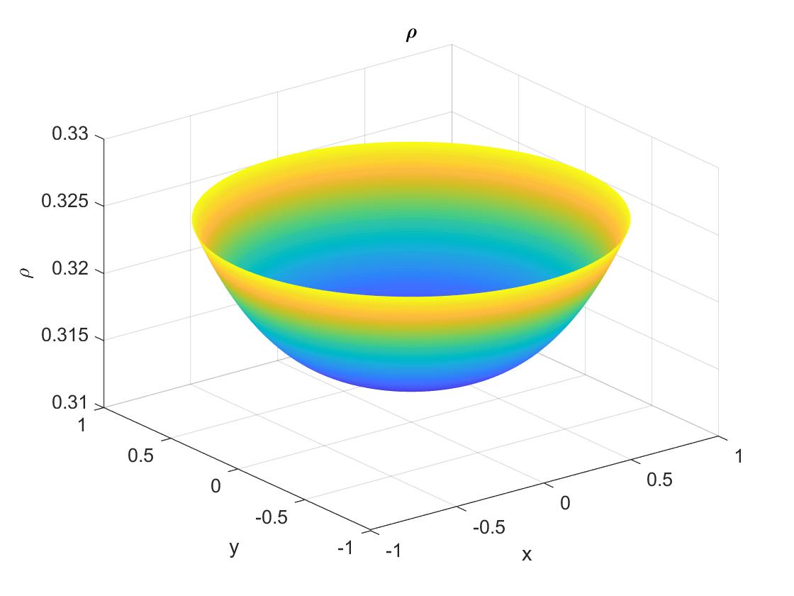
Figure 1: Charge distribution without external field, $u=0$.

In Example 1, we take $V=-\exp{\Big{(}-\frac{r^{2}}{2(0.05)^{2}}\Big{)}}$. The algorithm converges to a minimum after $100$ iterates. The valley function and the resulting plasma distribution are depicted in Figure 2. In Figure 3, we plot the control field $u$ and the self-consistent potential $U$.

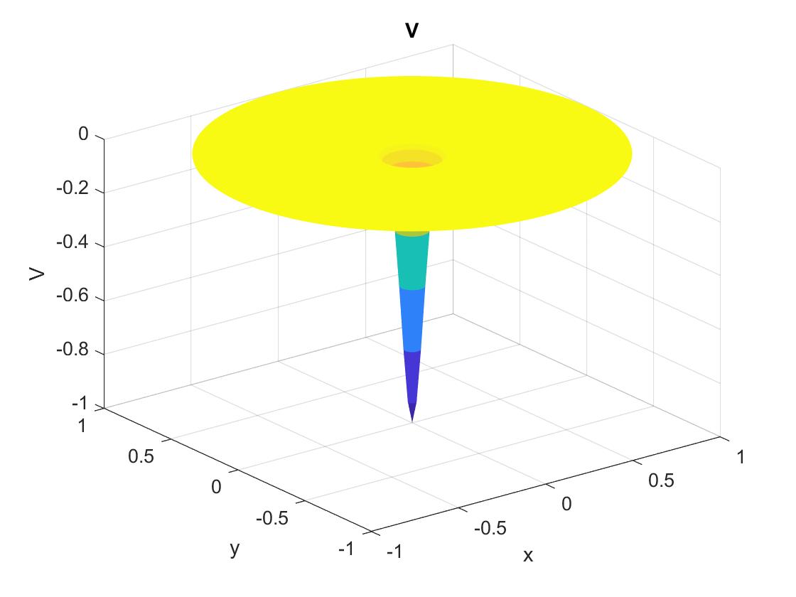
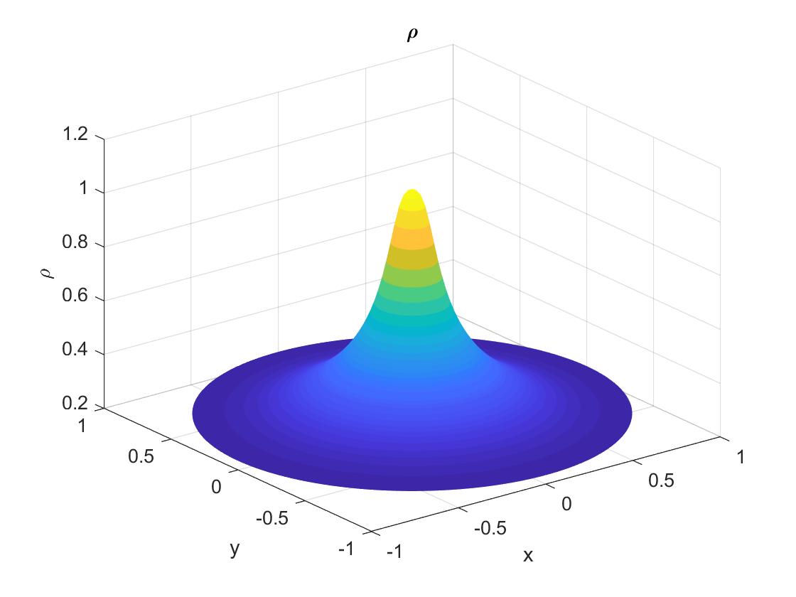
Figure 2: Left: Valley function. Right: Charge distribution. The figure refers to Example 1.

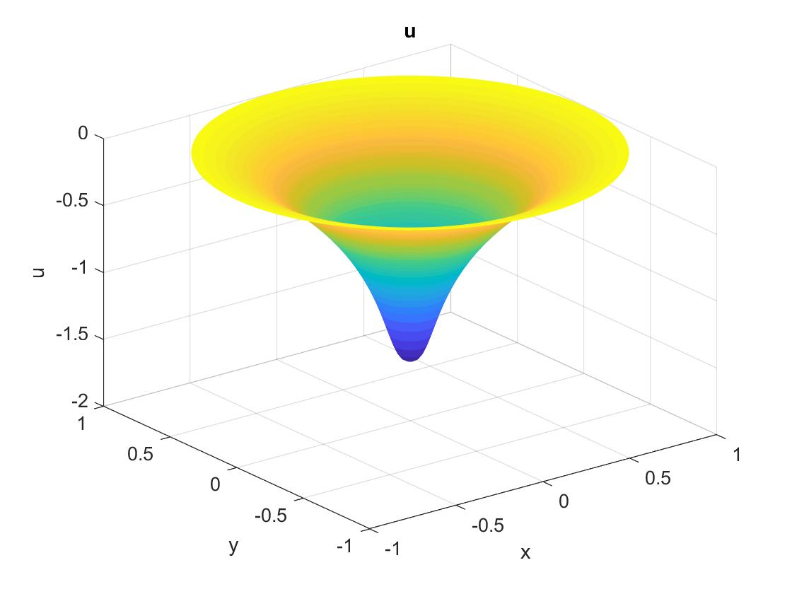
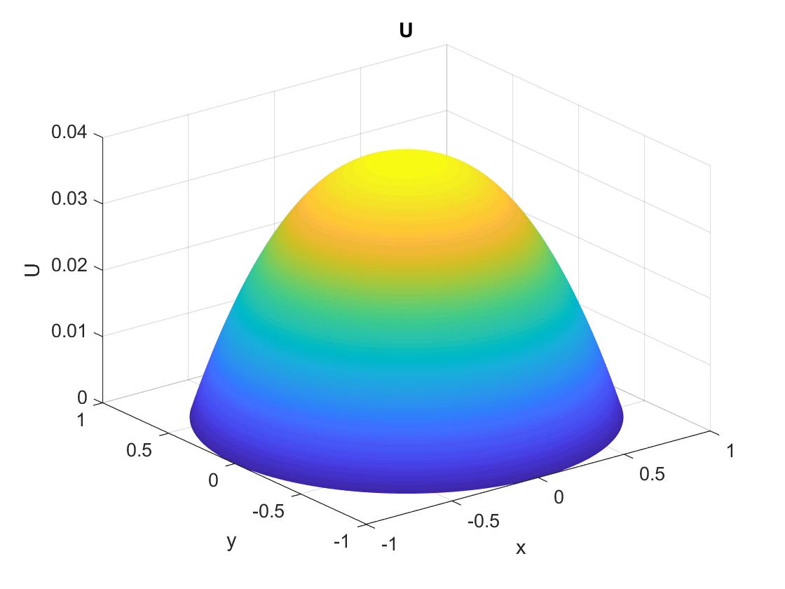
Figure 3: Left: External potential. Right: Self-consistent potential. The figure refers to Example 1.

In Example 2, we consider $V=-\exp{\Big{[}-r^{2}\Big{(}\frac{\cos^{2}{(\varphi)}}{2(0.05)^{2}}+\frac{\sin^{2}{(\varphi)}}{2(0.15)^{2}}\Big{)}\Big{]}}$. The algorithm converges to a minimum after $67$ iterates. The valley function and the resulting plasma distribution are depicted in Figure 4. In Figure 5, we plot the control field $u$ and the self-consistent potential $U$.

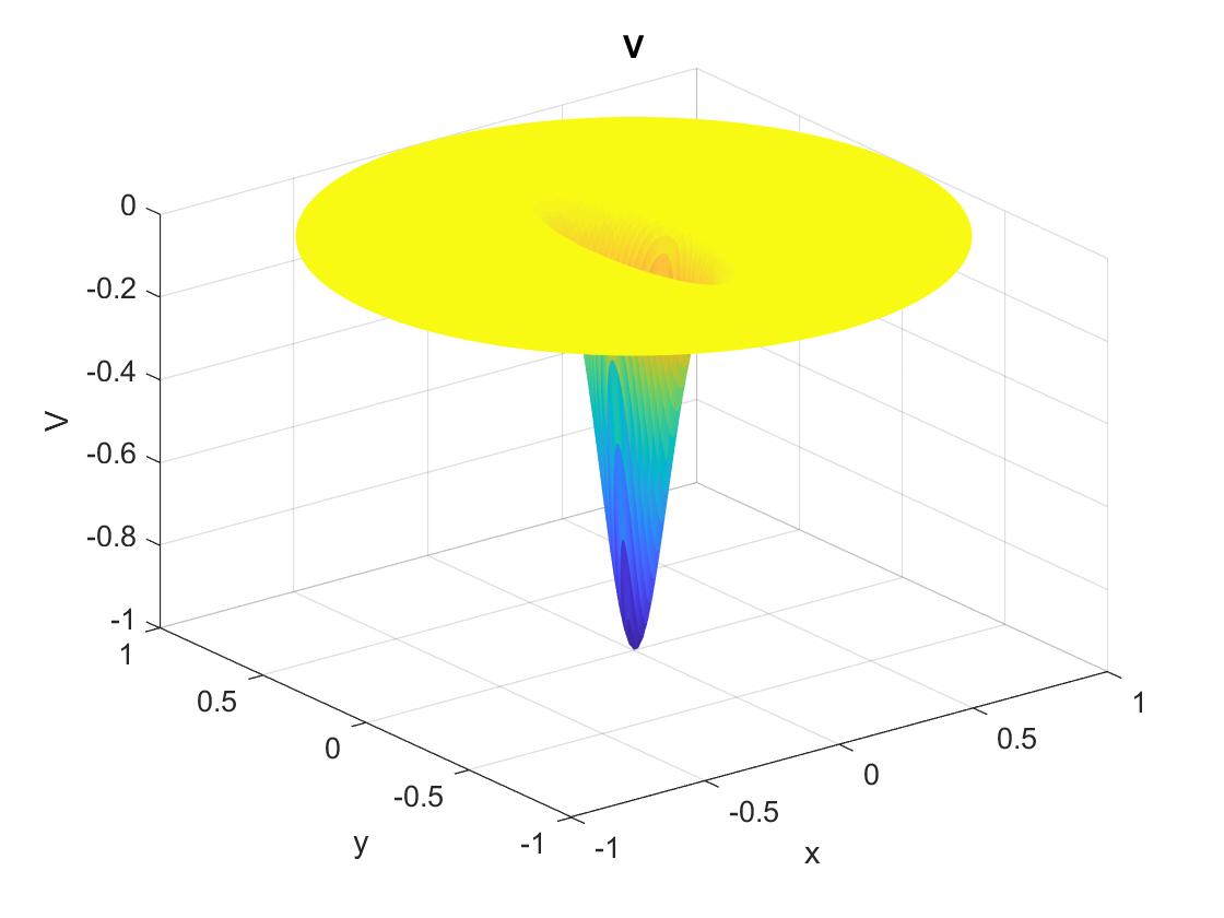
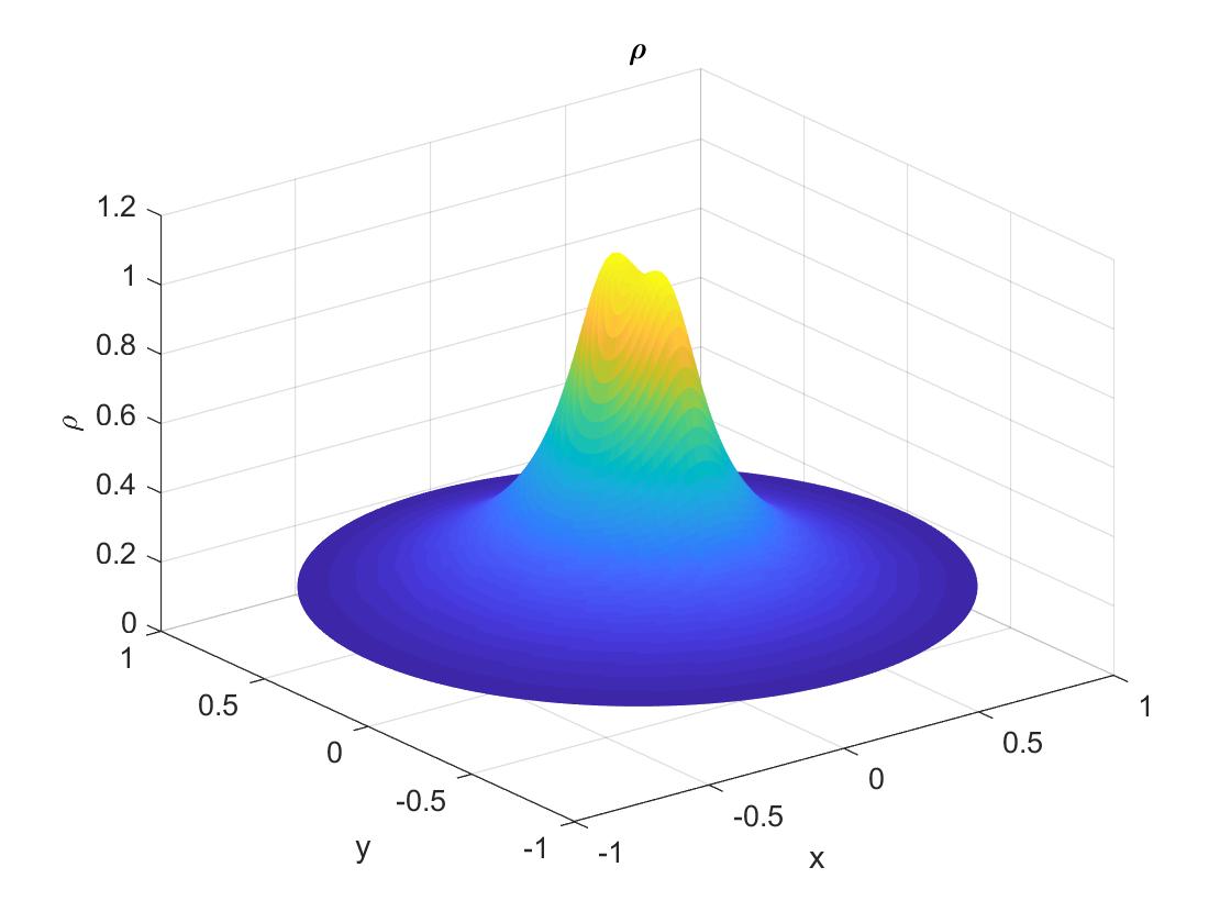
Figure 4: Left: Valley function. Right: Charge distribution. The figure refers to Example 2.

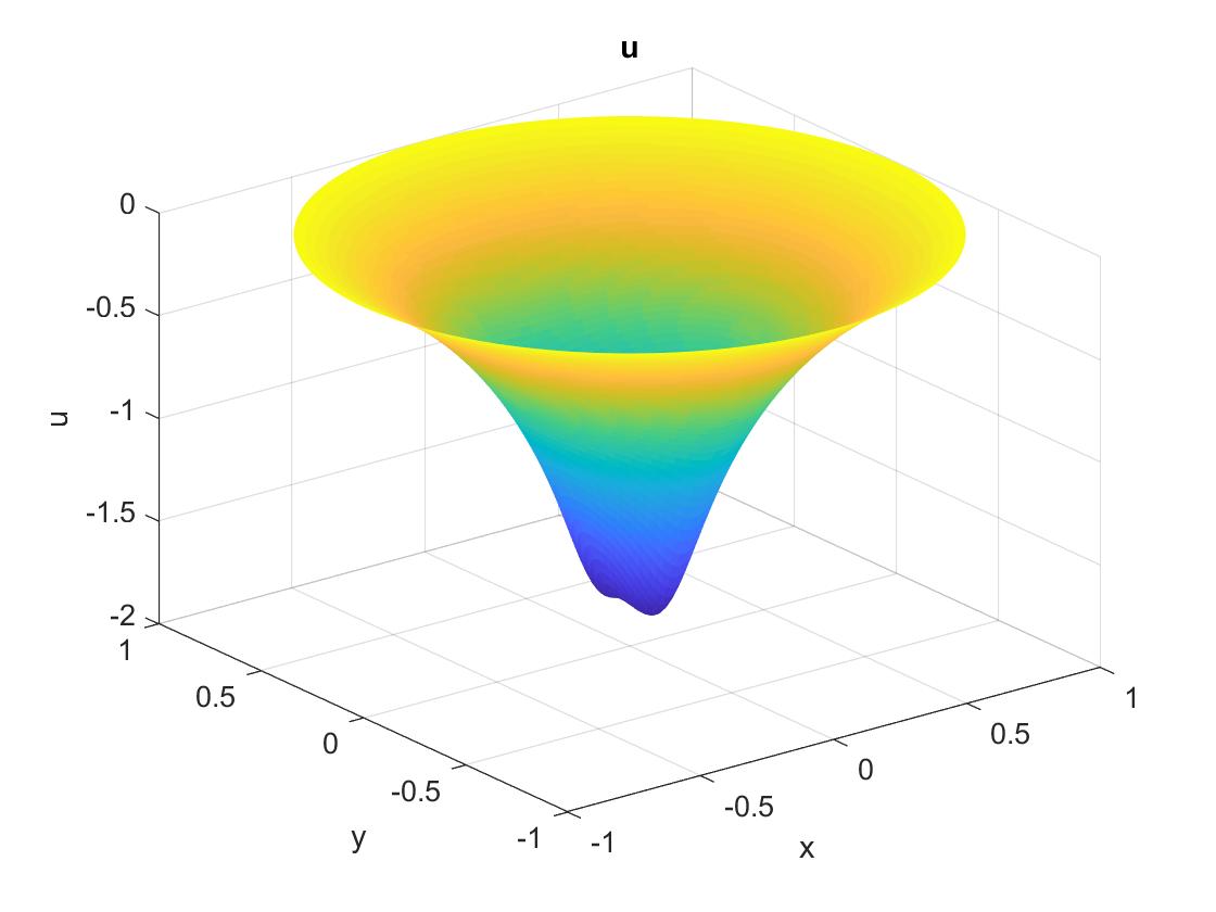
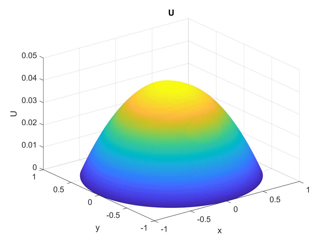
Figure 5: Left: External potential. Right: Self-consistent potential. The figure refers to Example 2.

In Example 3, we take a discontinuous valley potential with $V=-1$ inside the four-leaf clover and $V=0$ outside it, see Fig.6. The algorithm converges to a minimum after $66$ iterates. The valley function and the resulting plasma distribution are depicted in Figure 7. In Figure 8, we plot the control field $u$ and the self-consistent potential $U$.

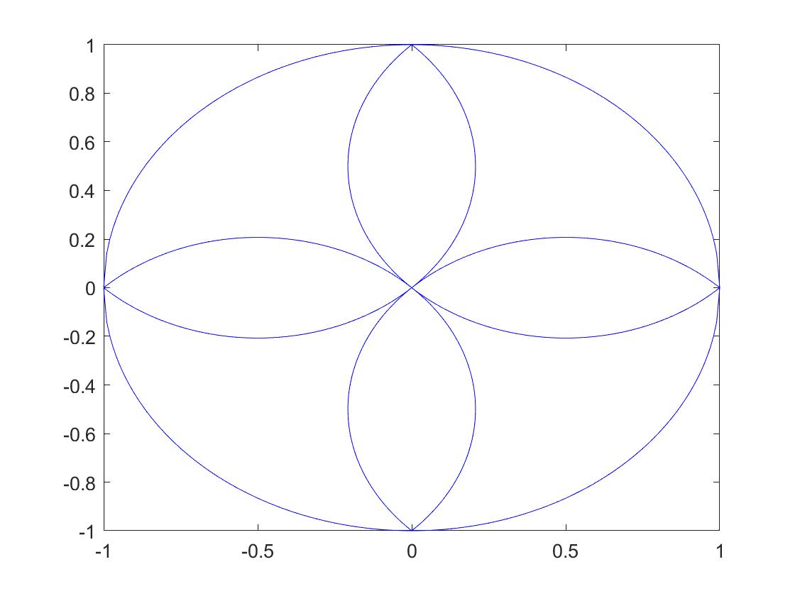
Figure 6: The cloverleaf inside of which $U=-1$ and outside of which $U=0$.

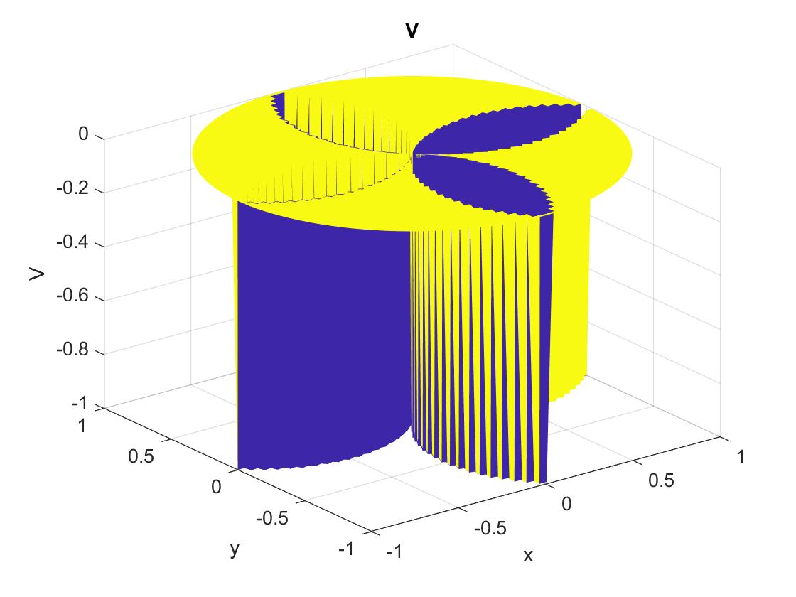
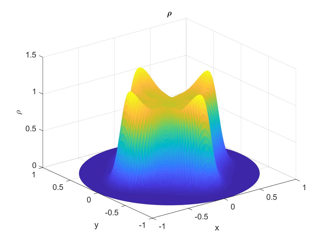
Figure 7: Left: Valley function. Right: Charge distribution. The figure refers to Example 3.

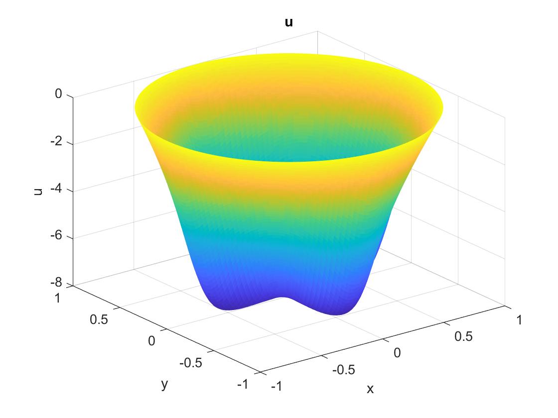
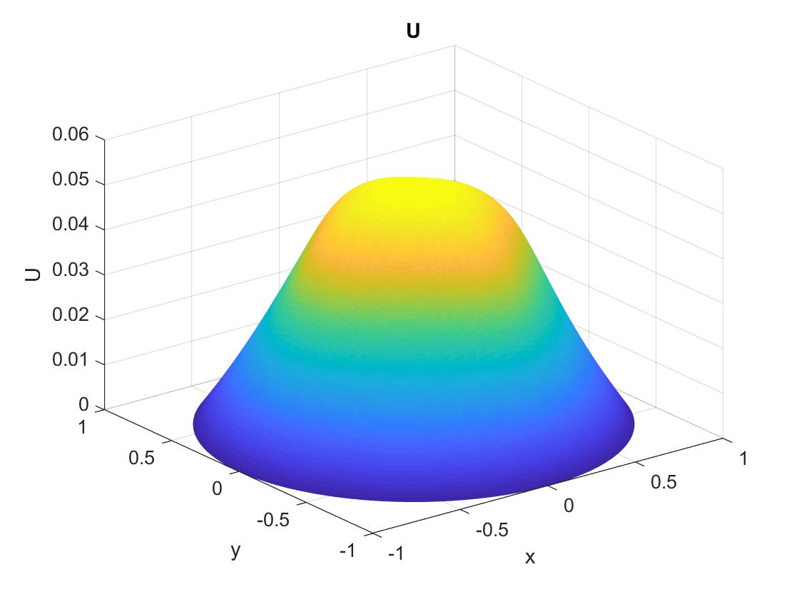
Figure 8: Left: External potential. Right: Self-consistent potential. The figure refers to Example 3.

We can see in the Figures 2, 4 and 7, that in all cases, the action of the external control field concentrates the plasma around the region where the valley function reaches its lower values, and its distribution reflects the geometrical properties of this function. On the other hand, without a control field the charge is mainly concentrated near the boundary of the domain as shown in Fig. 1.

Conclusion

This work was devoted to the formulation, theoretical investigation, and numerical solution of an optimal design problem for steady equilibrium solutions of the Vlasov-Poisson system where the design function is an external electric field.

The resulting optimization framework required to minimize an ensemble objective functional with Tikhonov regularization of the control field under the differential constraint of the nonlinear elliptic Poisson-Boltzmann equation that models equilibrium solutions of the Vlasov-Poisson system. Existence of optimal control fields and their characterization as solutions to first-order optimality conditions were discussed, and numerical approximation and optimization schemes were developed in order to compute these solutions. Results of numerical experiments were presented that successfully validated the proposed framework.

References

- [1] G. Manfredi and P.-A. Hervieux. Adiabatic cooling of trapped non-neutral plasmas. Phys. Rev. Lett., 109:255005, 2012.
- [2] S. Mazouffre. Electric propulsion for satellites and spacecraft: established technologies and novel approaches. Plasma Sources Science and Technology, 25(3):033002, apr 2016.
- [3] R. A. Dunlap. Energy from Nuclear Fusion. 2053-2563. IOP Publishing, 2021.
- [4] S.J. Doyle, D. Lopez-Aires, A. Mancini, M. Agredano-Torres, J.L. Garcia-Sanchez, J. Segado-Fernandez, J. Ayllon-Guerola, M. Garcia-Muñoz, E. Viezzer, C. Soria-Hoyo, J. Garcia-Lopez, G. Cunningham, P.F. Buxton, M.P. Gryaznevich, Y.S. Hwang, and K.J. Chung. Magnetic equilibrium design for the SMART tokamak. Fusion Engineering and Design, 171:112706, 2021.
- [5] H. Heumann, F. Rapetti, and X. Song. Finite element methods on composite meshes for tuning plasma equilibria in tokamaks. Journal of Mathematics in Industry, 8(1):8, 2018.
- [6] M. Holst, V. Kungurtsev, and S. Mukherjee. A note on optimal tokamak control for fusion power simulation. arXiv preprint arXiv:2211.08984, 2022.
- [7] P.-L. Lions and R. Di Perna. Solutions globales d’équations du type vlasov-poisson. Comptes rendus de l’Académie des sciences. Série 1, Mathématique, 307(12):655–658, 1988.
- [8] P. L. Lions and B. Perthame. Propagation of moments and regularity for the 3-dimensional Vlasov-Poisson system. Inventiones mathematicae, 105(1):415–430, 1991.
- [9] K. Pfaffelmoser. Global classical solutions of the vlasov-poisson system in three dimensions for general initial data. Journal of Differential Equations, 95(2):281–303, 1992.
- [10] A.A. Arsen’ev. Global existence of a weak solution of Vlasov’s system of equations. USSR Computational Mathematics and Mathematical Physics, 15(1):131–143, 1975.
- [11] E. Horst, R. Hunze, and H. Neunzert. Weak solutions of the initial value problem for the unmodified non-linear vlasov equation. Mathematical Methods in the Applied Sciences, 6(1):262–279, 1984.
- [12] F. Bavaud. Equilibrium properties of the Vlasov functional: The generalized Poisson-Boltzmann-Emden equation. Rev. Mod. Phys., 63:129–149, 1991.
- [13] J.A Carrillo. On a nonlocal elliptic equation with decreasing nonlinearity arising in plasma physics and heat conduction. Nonlinear Analysis: Theory, Methods & Applications, 32(1):97–115, 1998.
- [14] L. Desvillettes and J. Dolbeault. On long time asymptotics of the Vlasov—Poisson—Boltzmann equation. Communications in Partial Differential Equations, 16(2-3):451–489, 1991.
- [15] D. Gogny and P.-L. Lions. Sur les états d’équilibre pour les densités électroniques dans les plasmas. M2AN - Modélisation mathématique et analyse numérique, 23(1):137–153, 1989.
- [16] R. W. Brockett. Notes on the control of the Liouville equation. In Control of partial differential equations, volume 2048 of Lecture Notes in Math., pages 101–129. Springer, Heidelberg, 2012.
- [17] J. Bartsch, G. Nastasi, and A. Borzì. Optimal control of the Keilson-Storer master equation in a Monte Carlo framework. Journal of Computational and Theoretical Transport, 50(5):454–482, 2021.
- [18] J. Bartsch, A. Borzì, F. Fanelli, and S. Roy. A theoretical investigation of Brockett’s ensemble optimal control problems. Calculus of Variations and Partial Differential Equations, 58(5):162, 2019.
- [19] J. Bartsch, A. Borzì, F. Fanelli, and S. Roy. A numerical investigation of Brockett’s ensemble optimal control problems. Numerische Mathematik, 149(1):1–42, 2021.
- [20] R.C. Aster, B. Borchers, and C.H. Thurber. Parameter Estimation and Inverse Problems. Elsevier Science, 2013.
- [21] A.A. Vlasov. The vibrational properties of an electron gas. Usp. Fiz. Nauk, 93(3-4):444–470, 1967.
- [22] J. Dolbeault. Stationary states in plasma physics: Maxwellian solutions of the Vlasov-Poisson system. Mathematical Models and Methods in Applied Sciences, 1(2):183–208, 1991.
- [23] L. C. Evans. Partial Differential Equations. American Mathematical Society, 2010.
- [24] M. Annunziato and A. Borzì. A Fokker–Planck approach to the reconstruction of a cell membrane potential. SIAM Journal on Scientific Computing, 43(3):B623–B649, 2021.
- [25] S. Kullback and R. A. Leibler. On information and sufficiency. Ann. Math. Statist., 22(1):79–86, 03 1951.
- [26] J.-L. Lions. Optimal control of systems governed by partial differential equations. Translated from the French by S. K. Mitter. Die Grundlehren der mathematischen Wissenschaften, Band 170. Springer-Verlag, New York-Berlin, 1971.
- [27] F. Tröltzsch. Optimal Control of Partial Differential Equations, volume 112 of Graduate Studies in Mathematics. American Mathematical Society, Providence, RI, 2010.
- [28] R. A. Adams and J. J. F. Fournier. Sobolev Spaces, volume 140 of Pure and Applied Mathematics (Amsterdam). Elsevier/Academic Press, Amsterdam, second edition, 2003.
- [29] A. S. Reimer and A. F. Cheviakov. A Matlab-based finite-difference solver for the Poisson problem with mixed Dirichlet-Neumann boundary conditions. Comput. Phys. Commun., 184(3):783–798, 2013.
- [30] A. Borzì and V. Schulz. Computational Optimization of Systems Governed by Partial Differential Equations. Society for Industrial and Applied Mathematics, 2011.