Exploring semi-inclusive two-nucleon emission in neutrino scattering: a factorized approximation approach

Abstract

The semi-inclusive cross section of two-nucleon emission induced by neutrinos and antineutrinos is computed employing the relativistic mean field model of nuclear matter and the dynamics of meson exchange currents. Within this model we explore a factorization approximation based on the product of an integrated two-hole spectral function and a two-nucleon cross section averaged over hole pairs. We demonstrate that the integrated spectral function of the uncorrelated Fermi gas can be analytically computed, and we derive a simple fully relativistic formula for this function, showcasing its dependency solely on both missing momentum and missing energy. A prescription for the average momenta of the two holes in the factorized two-nucleon cross section is provided, assuming that these momenta are perpendicular to the missing momentum in the center-of-mass system. The validity of the factorized approach is assessed by comparing it with the unfactorized calculation. Our investigation includes the study of the semi-inclusive cross section integrated over the energy of one of the emitted nucleons and the cross section integrated over the emission angles of the two nucleons and the outgoing muon kinematics. A comparison is made with the pure phase-space model and other models from the literature. The results of this analysis offer valuable insights into the influence of the semi-inclusive hadronic tensor on the cross section, providing a deeper understanding of the underlying nuclear processes.

I Introduction

The investigation of two-nucleon emission in nuclear reactions induced by neutrinos has gained significance, particularly in modeling the inclusive quasielastic cross section at intermediate and high energies. Various model calculations Mar09 ; Mar10 ; Ama11 ; Nie11 ; Cuy16 ; Cuy17 ; Roc19 ; Mar21b ; Mar23b have indicated that multiparticle emission contribute significantly, accounting for approximately 20% or more of the quasielastic cross section, which is primarily dominated by one-particle emission. Consequently, the analysis of neutrino long-baseline experiments Gal11 ; Mor12 ; For12 ; Alv14 ; Mos16 ; Ath23 requires the consideration of two-particle two-hole (2p2h) emission events to accurately reconstruct the neutrino energy Sob20 .

In fact, commonly used Monte Carlo event generators such as GENIE Dol20 , NEUT Hay09 , NUWRO Jus09 ; Sto17 or GiBUU Lal12 , have incorporated the 2p2h channel from different models to account for this contribution. Typically, these generators include tables of the inclusive hadronic tensor $W^{\mu\nu}(q,\omega)$ as a function of momentum $q$ and energy transfer $\omega$, which are calculated and provided by the theoretical groups. Models from Lyon Mar09 , Valencia Nie11 , and Granada Sim17 are currently implemented in some of these generators, and although these models may significantly differ depending on the kinematics, these differences prove useful in refining the estimate of systematic errors in Monte Carlo (MC) outputs Val06 .

The implementation of the two-nucleon emission channel requires knowledge of the distribution of the two outgoing nucleons as functions of their outgoing momenta $\mathbf{p}^{\prime}_{1}$ and $\mathbf{p}^{\prime}_{2}$, for the proton-proton (pp), proton-neutron (pn), and neutron-neutron (nn) channels. In the absence of a model for the semi-inclusive 2p2h cross section, a first approximation is to assume isotropic symmetry in the center-of-mass (CM) system of the outgoing particles Sob12 when the emitted pair of nucleons absorbs momentum $q$ and energy $\omega$. The corresponding distribution is normalized using the inclusive cross section Dol20 . However, angular symmetry in the CM is broken due to the interaction, as the electroweak current matrix element depends non-trivially on the moments of the initial and final particles Sim17 . To determine the extent to which the isotropy is broken, a more realistic model for the semi-inclusive two-nucleon emission reaction is needed, which should be relativistic given the momenta and energies involved in neutrino experiments, of the order of 1 GeV.

In independent-particle nuclear models, the emission of two particles with neutrinos requires two-body current operators. These currents are commonly modeled by assuming meson exchange between nucleons, where the neutrino interacts with a pair of nucleons exchanging a meson. These are known as meson exchange currents (MEC) and involve a series of diagrams describing interactions with the exchanged meson, possibly with the excitation of a nucleon resonance $\Delta(1232)$, with vector and axial contributions Tow87 ; Ris89 . Since the MEC contain the excitation of an intermediate $\Delta$, this extends the kinematic domain of the 2p2h inclusive response, as a function of the energy transfer, from the quasielastic peak and beyond, up to the $\Delta$ peak Mai09 . In more realistic nuclear models, nucleon-nucleon correlations also allow the emission of two particles with the one-body current, leading to interferences between the one-body and two-body currents Roc19 ; Roc19b ; Ben15 ; Ben23 .

Up to now, most models of 2p2h emission with neutrinos have focused on calculating the inclusive reaction. The study of semi-inclusive processes has, until recently, predominantly focused on one-particle emission due to its major contribution to the quasielastic cross section Fra20 ; Fra21 ; Bar21 ; Fra22 ; Fra22b ; Fra23 . Early attempts to compute a semi-inclusive cross section with multinucleon knockout were limited to the non-relativistic shell model, as seen in the work of Cuy16 ; Cuy17 , and the calculation presented in Sob20 using the relativistic Fermi gas with a local density approximation. In Cuy17 , a MEC model was employed for the two-body current, excluding the $\Delta$ excitation current, and the final state interaction was considered with a real single-particle potential. Meanwhile, in Sob20 , a relativistic model based on a many-body formalism was applied, and the final-state interaction was modeled by the cascade model implemented in the NEUT generator.

We have recently introduced a model for semi-inclusive two-nucleon emission induced by neutrinos Mar24 . Our approach relies on the relativistic mean field of nuclear matter (RMF) and incorporates relativistic MEC operators, including seagull, pion-in-flight (pionic), pion-pole, and $\Delta$ isobar currents. This model has been developed across a series of works Mar21a ; Mar21b ; Mar23a to compute the inclusive cross section in the 2p2h channel, in conjunction with the superscaling approach with relativistic effective mass (SuSAM*). Our efforts culminated in a systematic analysis of available experimental quasielastic scattering data of neutrinos, demonstrating reasonable agreement with the experimental results Mar23b similar to other different approaches Meg13 .

The next logical step in this framework would be to extend the same MEC model within the RMF to predict the semi-inclusive cross section consistently with the inclusive 2p2h cross section. In fact, we have already applied this approach to the semi-inclusive 2p2h reaction in Mar24 for neutrino and antineutrino scattering, where we explored the one-fold and two-fold cross sections obtained by integrating over four or five of the variables associated with the final momenta $p^{\prime}_{1}$ and $p^{\prime}_{2}$. In Mar24 we have detailed the implications of using the RMF microscopic approach, which involves asymmetric distributions of nucleons in the CM system of the final state, in contrast to oversimplified modeling where isotropic distributions are assumed. Clear differences have been observed, which should have important implications for Monte Carlo analyses of neutrino reactions. Additionally, focus was placed on the distributions of proton-proton, proton-neutron and neutron-neutron pairs, and, again, important differences were observed for the microscopical approach versus the results found in the naive symmetric modeling.

In this work, we continue this study by analyzing other aspects of semi-inclusive cross sections for two-nucleon emission:

1. We will study the more general 5-folded cross section by integrating over the energy of one of the final nucleons while keeping constant the emission angles and the energy of the other nucleon. This will allow us to compare with the calculations of Cuy17 in the shell model, where MECs were considered without the $\Delta$ current. Here, we can observe the effect of MEC separately.

2. We are going to explore a factorized approximation as the product of a two-nucleon cross section multiplied by an integrated spectral function. This will allow us to see if factorized models developed for electron scattering from correlated nuclei, where the cross section is factored as the product of the one-body current by a combination of two-hole spectral functions, can be extended to the case of MEC Geu96 ; Ben99 . We will see that in the RMF, the integrated spectral function admits an analytical formula, simplifying the calculations. We will demonstrate that the two-nucleon cross section can be estimated using a prescription that fixes the average momenta of the holes.

3. Using the factorized formula, we will be able to calculate the cross section integrated over the outgoing muon and the angles of the final nucleons. This will allow us to compare with the calculation in Ref. Sob20 , where a microscopic calculation of this observable was performed and compared with the result from the NEUT event generator.

4. Finally, for all these observables, we will compare with the isotropic symmetric model and study the differences with our microscopic model.

In Section 2, we summarize the formalism of semi-inclusive two-particle emission in the RMF. In Section 3, we introduce the factorized approximation. In Section 4, we present the results for the 5-folded cross section and for the cross section integrated over the final muon and the nucleon angles. In Section 5, we draw our conclusions. In the appendix, we present some mathematical details on the derivation of the integrated two-hole spectral function.

II Formalism

II.1 Semi-inclusive 2p2h cross section

Here we summarize the formalism used to describe the semi-inclusive charge-changing (CC) reactions induced by neutrinos, $(\nu_{\mu},\mu^{-}N_{1}N_{2})$, and antineutrinos, $(\overline{\nu}_{\mu},\mu^{+}N_{1}N_{2})$, in which two nucleons are detected in coincidence with the muon. The residual daughter A-2 nucleus state is not detected. This is why we use the convention to call this reaction semi-inclusive, in contrast to the inclusive reaction in which only the lepton is detected, and the exclusive reaction where the state of the daughter nucleus is also known, and therefore, the hadronic final state is completely specified.

We closely follow the formalism of Ref. Mar24 that contains more details on the model. The incident neutrino has four-momentum $k^{\mu}=(\epsilon,\mathbf{k})$, and the final muon has $k^{\prime}{}^{\mu}=(\epsilon^{\prime},\mathbf{k^{\prime}})$. The energy transfer is $\omega=(\epsilon-\epsilon^{\prime})$ and the momentum transfer is $\mathbf{q}=(\mathbf{k}-\mathbf{k^{\prime}})$, with $Q^{2}=\omega^{2}-|\mathbf{q}|^{2}<0$. The corresponding differential cross-section for detecting a muon with kinetic energy $T_{\mu}$ within a solid angle $\Omega_{\mu}=(\theta_{\mu},\phi_{\mu})$ and two nucleons with momenta $\mathbf{p}^{\prime}_{1}$ and $\mathbf{p}^{\prime}_{2}$ can be written as

$$\frac{d\sigma_{N_{1}N_{2}}}{dT_{\mu}d\Omega_{\mu}d^{3}p^{\prime}_{1}d^{3}p^{\prime}_{2}}=\sigma_{0}L_{\mu\nu}W^{\mu\nu}_{N_{1}N_{2}}({\bf p}^{\prime}_{1},{\bf p}^{\prime}_{2},{\bf q},\omega)$$ (1)

where the function $\sigma_{0}$ is given by

$$\sigma_{0}(k,k^{\prime})=\frac{G^{2}\cos^{2}\theta_{c}}{4\pi^{2}}\frac{k^{\prime}}{k}$$ (2)

In this equation the Fermi constant is $G=1.166\times 10^{-11}\quad\rm MeV^{-2}$, and the cosine of the Cabibbo angle is $\cos\theta_{c}=0.975$.

In Eq. (1) the leptonic tensor, $L_{\mu\nu}$, is given by:

$$L_{\mu\nu} = k_{\mu}k^{\prime}_{\nu}+k_{\nu}k^{\prime}_{\mu}-kk^{\prime}g_{\mu\nu}\pm i\epsilon_{\mu\nu\alpha\beta}k^{\alpha}k^{\prime\beta}$$ (3)

where the sign $+(-)$ is for neutrino (antineutrino) scattering. Finally, in Eq. (1) the leptonic tensor is contracted with the semi-inclusive hadronic tensor, $W^{\mu\nu}_{N_{1}N_{2}}({\bf p}^{\prime}_{1},{\bf p}^{\prime}_{2},{\bf q},\omega)$, that contains the information about the nuclear model of the reaction, for emitting a pair of nucleons with charges $N_{1},N_{2}$, and momenta $({\bf p}^{\prime}_{1},{\bf p}^{\prime}_{2})$, in an electroweak interaction that transfers energy-momentum $(\omega,{\bf q})$. In this work, we will compute this tensor using the RMF of nuclear matter.

In the RMF framework the nucleons interact with scalar and vector potentials, represented as $g_{s}\phi_{0}$ and $g_{v}V_{0}$ respectively Ros80 ; Ser86 ; Weh93 . These potentials capture the strong interaction forces among nucleons within the nuclear medium. The RMF model treats nucleons as interacting with these potentials, resulting in effective masses for nucleons denoted as $m_{N}^{*}=m_{N}-g_{s}\phi_{0}$. The effective mass considers the modification of the nucleon’s mass due to the scalar potential, while the vector potential contributes a repulsive vector energy, $E_{v}=g_{v}V_{0}$. In the RMF formalism the on-shell energy of a nucleon with momentum ${\bf p}$ is defined as

$$E=\sqrt{p^{2}+m_{N}^{*2}},\kern 28.45274ptm_{N}^{*}=m_{N}-g_{s}\phi_{0},$$ (4)

while the true total energy of the nucleon in the RMF is given by

$$E_{RMF}=E+E_{v}=E+g_{v}V_{0}$$ (5)

In this approach, the single nucleon states are plane waves $u_{s}({\bf p})e^{i{\bf p}\cdot{\bf r}}$, where the spinor $u_{s}({\bf p})$ is a solution of the Dirac equation with mass $m_{N}^{*}$. The ground state nuclear wave function of the Fermi gas, $|F\rangle$, is constructed as a Slater determinant with all levels occupied below some Fermi momentum $k_{F}$. Consequently, the action of a two-body operator associated with the weak interaction can excite this ground state, generating two-particle two-hole excitations (2p2h) and leading to the emission of two particles.

$$|F\rangle\rightarrow|1^{\prime},2^{\prime},1^{-1},2^{-1}\rangle=a^{\dagger}_{1^{\prime}}a^{\dagger}_{2^{\prime}}a_{1}a_{2}|F\rangle.$$ (6)

The operators $a_{i^{\prime}}^{\dagger}$ and $a_{i}$ are creation and annihilation operators for single-particle states where the states with and without prime correspond to particles and holes, respectively, including spin and isospin indices

$$|i\rangle=|{\bf h}_{i},s_{i},t_{i}\rangle,\kern 28.45274pt|i^{\prime}\rangle=|{\bf p}^{\prime}_{i},s^{\prime}_{i},t^{\prime}_{i}\rangle,\kern 28.45274pti=1,2.$$ (7)

Applying the RMF model to the semi-inclusive two-particle emission results in the following formula for the semi-inclusive hadronic tensor Mar24

$$W^{\mu\nu}_{N_{1}N_{2}}({\bf p}^{\prime}_{1},{\bf p}^{\prime}_{2},{\bf q},\omega) = \frac{V}{(2\pi)^{9}}\int d^{3}h_{1}d^{3}h_{2}\frac{(m^{*}_{N})^{4}}{E_{1}E_{2}E^{\prime}_{1}E^{\prime}_{2}}w^{\mu\nu}_{N_{1}N_{2}}({\bf p}^{\prime}_{1},{\bf p}^{\prime}_{2},{\bf h}_{1},{\bf h}_{2})\delta(E^{\prime}_{1}+E^{\prime}_{2}-E_{1}-E_{2}-\omega)$$ (8)

$$\times\delta({\bf p}^{\prime}_{1}+{\bf p}^{\prime}_{2}-{\bf h}_{1}-{\bf h}_{2}-{\bf q})\theta(p^{\prime}_{1}-k_{F})\theta(p^{\prime}_{2}-k_{F})\theta(k_{F}-h_{1})\theta(k_{F}-h_{2}),$$

where $w^{\mu\nu}_{N_{1}N_{2}}({\bf p}^{\prime}_{1},{\bf p}^{\prime}_{2},{\bf h}_{1},{\bf h}_{2})$ represents the elementary 2p2h hadronic tensor, and $V/(2\pi)^{3}=Z/(\frac{8}{3}\pi k_{F}^{3})$ for symmetric nuclear matter. The delta functions ensure energy-momentum conservation in the 2p2h excitation

$${\bf p}^{\prime}_{1}+{\bf p}^{\prime}_{2}={\bf q}+{\bf h}_{1}+{\bf h}_{2},\kern 28.45274ptE^{\prime}_{1}+E^{\prime}_{2}=\omega+E_{1}+E_{2}.$$ (9)

In Eq. (8) the product of step functions impose Pauli blocking restrictions on the momenta of the particles and holes, ensuring that the final momenta (${\bf p}^{\prime}_{i}$) are larger than the Fermi momentum ($k_{F}$), indicating that they are excited states above the Fermi surface, and similarly, the momenta of the holes (${\bf h}_{2}$) are smaller than the Fermi momentum, indicating that they are occupied states below the Fermi surface.

The elementary 2p2h hadronic tensor describes the transitions between two holes and two particles

$$|1,2\rangle\longrightarrow|1^{\prime},2^{\prime}\rangle$$ (10)

produced by the two-body current operator with matrix elements Ama02

$$\langle 1^{\prime}2^{\prime}|J^{\mu}({\bf q},\omega)|12\rangle=\frac{(2\pi)^{3}}{V^{2}}\frac{(m_{N}^{*})^{2}}{\sqrt{E^{\prime}_{1}E^{\prime}_{2}E_{1}E_{2}}}\delta({\bf p}^{\prime}_{1}+{\bf p}^{\prime}_{2}-{\bf h}_{1}-{\bf h}_{2}-{\bf q})j^{\mu}(1^{\prime},2^{\prime},1,2),$$ (11)

where the current functions $j^{\mu}(1^{\prime},2^{\prime},1,2)$ are described below. The elementary 2p2h hadronic tensor is defined by

$$w^{\mu\nu}_{N_{1}N_{2}}({\bf p}^{\prime}_{1},{\bf p}^{\prime}_{2},{\bf h}_{1},{\bf h}_{2})=\frac{1}{2}\sum_{s_{1}s_{2}s^{\prime}_{1}s^{\prime}_{2}}j^{\mu}(1^{\prime},2^{\prime},1,2)^{*}_{A}\,j^{\nu}(1^{\prime},2^{\prime},1,2)_{A}\,.$$ (12)

where we sum over all possible spin projections of the spin-1/2 nucleons in the 2p2h excitation, as we consider the non-polarized case where the nucleon spins are not measured. The factor $1/2$ in Eq. (12) is included to avoid double counting when summing over spin, due to the antisymmetry of the two-body wave function with respect to the pp or nn pair. The two-body current matrix element is antisymmetrized with respect to identical particles. For the specific process $\nu_{\mu}nn\rightarrow\mu^{-}pn$, the antisymmetrization is as follows:

$$j^{\mu}(1^{\prime},2^{\prime},1,2)_{A}=j^{\mu}(1^{\prime},2^{\prime},1,2)-j^{\mu}(1^{\prime},2^{\prime},2,1),$$ (13)

and for $\nu_{\mu}pn\rightarrow\mu^{-}pp$,

$$j^{\mu}(1^{\prime},2^{\prime},1,2)_{A}=j^{\mu}(1^{\prime},2^{\prime},1,2)-j^{\mu}(2^{\prime},1^{\prime},1,2).$$ (14)

There are similar expressions for the antineutrino case.

II.2 Meson-exchange currents

In this work, we use the electroweak MEC model described by the nine Feynman diagrams depicted in Fig. 1. The two-body current matrix elements $j^{\mu}(1^{\prime},2^{\prime},1,2)$ corresponding to this model enter in the calculation of the elementary 2p2h hadronic tensor, Eq. (12). The different contributions have been taken from the pion weak production model of ref. Her07 . The MEC is the sum of four two-body operators: seagull (diagrams a, b), pion in flight (c), pion-pole (d, e), and $\Delta(1232)$ excitation forward (f, g) and backward (h, i). In the MEC model, we don’t include the correlation currents that follow from the nucleon pole diagrams of Her07 : those currents present divergence problems due to the double pole in the nucleon propagator Alb84 ; Ama10 and don’t properly account for nuclear correlations realistically because they only involve the exchange of one pion. A more realistic description of short-range correlations (SRC) requires using an effective nucleon-nucleon interaction Nie11 ; Gra13 . Alternatively in ref. Mar23a a theoretical description of correlation currents has been proposed requiring to solve the Bethe-Goldstone equation with a realistic nucleon-nucleon interaction, a challenge that needs further work and will be presented elsewhere. For this work, we focus on the genuine MEC 2p2h responses to connect with our previous works on inclusive 2p2h response Mar21a ; Mar21b ; Mar23b .

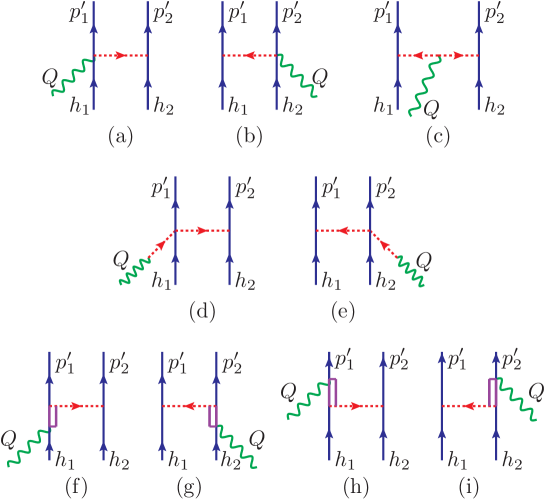
Figure 1: Feynman diagrams of meson exchange currents considered in the present work.

The relativistic MEC model for neutrino reactions was introduced in ref. Rui17 to study the 2p2h inclusive responses in the RFG and later extended in Mar21a ; Mar21b to the RMF, including the effective mass and the vector energy. Following ref. Rui17 , we explicitly separate the isospin matrix elements from the spatial and spin dependence. This compact form will be useful, as we will see later, for interpreting the results of semi-inclusive pn emission. The MEC depend on isospin across the three operators Rui17

$$\mbox{\boldmath$\tau$}^{(1)},\kern 28.45274pt\mbox{\boldmath$\tau$}^{(2)},\kern 28.45274pt\mbox{\boldmath$I$}_{V}\equiv i\left[\mbox{\boldmath$\tau$}^{(1)}\times\mbox{\boldmath$\tau$}^{(2)}\right],\\$$ (15)

that is, the isospin of the first and second particles and their vector product. Then neutrino or antineutrino CC scattering involves the $\pm$ components

$$\tau^{(1)}_{\pm} = \tau^{(1)}_{x}\pm i\tau^{(1)}_{y}$$ (16)

$$\tau^{(2)}_{\pm} = \tau^{(2)}_{x}\pm i\tau^{(2)}_{y}$$ (17)

$$I_{V\pm} = (I_{V})_{x}\pm i(I_{V})_{y}.$$ (18)

The MEC can be decomposed accordingly as a sum of at most three contributions. For neutrino scattering we have

$$j^{\mu}_{\rm sea} = \langle t^{\prime}_{1}t^{\prime}_{2}|I_{V+}(K_{S1}^{\mu}-K_{S2}^{\mu})|t_{1}t_{2}\rangle,$$ (19)

$$j^{\mu}_{\pi} = \langle t^{\prime}_{1}t^{\prime}_{2}|I_{V+}K_{\pi}^{\mu}|t_{1}t_{2}\rangle,$$ (20)

$$j^{\mu}_{\rm pole} = \langle t^{\prime}_{1}t^{\prime}_{2}|I_{V+}(K_{P1}^{\mu}-K_{P2}^{\mu})|t_{1}t_{2}\rangle,$$ (21)

$$j^{\mu}_{\Delta F} = \langle t^{\prime}_{1}t^{\prime}_{2}|\frac{1}{\sqrt{6}}\left[2\tau_{+}^{(2)}K_{F1}+2\tau_{+}^{(1)}K_{F2}-I_{V+}(K_{F1}-K_{F2})\right]|t_{1}t_{2}\rangle,$$ (22)

$$j^{\mu}_{\Delta B} = \langle t^{\prime}_{1}t^{\prime}_{2}|\frac{1}{\sqrt{6}}\left[2\tau_{+}^{(2)}K_{B1}+2\tau_{+}^{(1)}K_{B2}+I_{V+}(K_{B1}-K_{B2})\right]|t_{1}t_{2}\rangle,$$ (23)

and similar expressions with the minus (-) operators for antineutrino scattering. The nine functions $K^{\mu}_{S1}$, $K^{\mu}_{S2}$, $K^{\mu}_{\pi}$, $K^{\mu}_{P1}$, $K^{\mu}_{P1}$, $K^{\mu}_{F1}$, $K^{\mu}_{F2}$, $K^{\mu}_{B1}$, $K^{\mu}_{B2}$, only depend on momenta and spins $({\bf p}^{\prime}_{1}s^{\prime}_{1},{\bf p}^{\prime}_{2}s^{\prime}_{2},{\bf h}_{1}s_{1},{\bf h}_{2}s_{2})$. They are given by

$$K^{\mu}_{\rm S1}({\bf p}^{\prime}_{1}s^{\prime}_{1},{\bf p}^{\prime}_{2}s^{\prime}_{2},{\bf h}_{1}s_{1},{\bf h}_{2}s_{2}) = \frac{f_{\pi NN}^{2}}{m^{2}_{\pi}}V_{\pi NN}^{s^{\prime}_{1}s_{1}}({\bf p}^{\prime}_{1},{\bf h}_{1})F_{\pi NN}(k_{1}^{2})\bar{u}_{s^{\prime}_{2}}({\bf p}^{\prime}_{2})\left[F^{V}_{1}(Q^{2})\gamma_{5}\gamma^{\mu}+\frac{F_{\rho}\left(k_{2}^{2}\right)}{g_{A}}\,\gamma^{\mu}\right]u_{s_{2}}({\bf h}_{2}),$$ (24)

$$K^{\mu}_{\rm S2}({\bf p}^{\prime}_{1}s^{\prime}_{1},{\bf p}^{\prime}_{2}s^{\prime}_{2},{\bf h}_{1}s_{1},{\bf h}_{2}s_{2}) = K^{\mu}_{\rm S1}({\bf p}^{\prime}_{2}s^{\prime}_{2},{\bf p}^{\prime}_{1}s^{\prime}_{1},{\bf h}_{2}s_{2},{\bf h}_{1}s_{1}),$$ (25)

$$K^{\mu}_{\pi}({\bf p}^{\prime}_{1}s^{\prime}_{1},{\bf p}^{\prime}_{2}s^{\prime}_{2},{\bf h}_{1}s_{1},{\bf h}_{2}s_{2}) = \frac{f_{\pi NN}^{2}}{m^{2}_{\pi}}F^{V}_{1}(Q^{2})V_{\pi NN}^{s^{\prime}_{1}s_{1}}({\bf p}^{\prime}_{1},{\bf h}_{1})V_{\pi NN}^{s^{\prime}_{2}s_{2}}({\bf p}^{\prime}_{2},{\bf h}_{2})\left(k^{\mu}_{1}-k^{\mu}_{2}\right),$$ (26)

$$K^{\mu}_{\rm P1}({\bf p}^{\prime}_{1}s^{\prime}_{1},{\bf p}^{\prime}_{2}s^{\prime}_{2},{\bf h}_{1}s_{1},{\bf h}_{2}s_{2}) = \frac{f_{\pi NN}^{2}}{m^{2}_{\pi}}\,\frac{F_{\rho}\left(k_{1}^{2}\right)}{g_{A}}F_{\pi NN}(k_{2}^{2})\frac{Q^{\mu}\bar{u}_{s^{\prime}_{1}}({\bf p}^{\prime}_{1})\not{\!Q}u_{s_{1}}({\bf h}_{1})}{Q^{2}-m^{2}_{\pi}}V_{\pi NN}^{s^{\prime}_{2}s_{2}}({\bf p}^{\prime}_{2},{\bf h}_{2}),$$ (27)

$$K^{\mu}_{\rm P2}({\bf p}^{\prime}_{1}s^{\prime}_{1},{\bf p}^{\prime}_{2}s^{\prime}_{2},{\bf h}_{1}s_{1},{\bf h}_{2}s_{2}) = K^{\mu}_{\rm P1}({\bf p}^{\prime}_{2}s^{\prime}_{2},{\bf p}^{\prime}_{1}s^{\prime}_{1},{\bf h}_{2}s_{2},{\bf h}_{1}s_{1}),$$ (28)

$$K^{\mu}_{F1}({\bf p}^{\prime}_{1}s^{\prime}_{1},{\bf p}^{\prime}_{2}s^{\prime}_{2},{\bf h}_{1}s_{1},{\bf h}_{2}s_{2}) = \frac{f^{*}f_{\pi NN}}{m^{2}_{\pi}}\,V_{\pi NN}^{s^{\prime}_{2}s_{2}}({\bf p}^{\prime}_{2},{\bf h}_{2})F_{\pi N\Delta}(k_{2}^{2})\bar{u}_{s^{\prime}_{1}}({\bf p}^{\prime}_{1})k^{\alpha}_{2}G_{\alpha\beta}(h_{1}+Q)\Gamma^{\beta\mu}(Q)u_{s_{1}}({\bf h}_{1}),$$ (29)

$$K^{\mu}_{\rm F2}({\bf p}^{\prime}_{1}s^{\prime}_{1},{\bf p}^{\prime}_{2}s^{\prime}_{2},{\bf h}_{1}s_{1},{\bf h}_{2}s_{2}) = K^{\mu}_{\rm F1}({\bf p}^{\prime}_{2}s^{\prime}_{2},{\bf p}^{\prime}_{1}s^{\prime}_{1},{\bf h}_{2}s_{2},{\bf h}_{1}s_{1}),$$ (30)

$$K^{\mu}_{B1}({\bf p}^{\prime}_{1}s^{\prime}_{1},{\bf p}^{\prime}_{2}s^{\prime}_{2},{\bf h}_{1}s_{1},{\bf h}_{2}s_{2}) = \frac{f^{*}f_{\pi NN}}{m^{2}_{\pi}}\,V_{\pi NN}^{s^{\prime}_{2}s_{2}}({\bf p}^{\prime}_{2},{\bf h}_{2})F_{\pi N\Delta}(k_{2}^{2})\bar{u}_{s^{\prime}_{1}}({\bf p}^{\prime}_{1})k^{\beta}_{2}\hat{\Gamma}^{\mu\alpha}(Q)G_{\alpha\beta}(p^{\prime}_{1}-Q)u_{s_{1}}({\bf h}_{1}),$$ (31)

$$K^{\mu}_{\rm B2}({\bf p}^{\prime}_{1}s^{\prime}_{1},{\bf p}^{\prime}_{2}s^{\prime}_{2},{\bf h}_{1}s_{1},{\bf h}_{2}s_{2}) = K^{\mu}_{\rm B1}({\bf p}^{\prime}_{2}s^{\prime}_{2},{\bf p}^{\prime}_{1}s^{\prime}_{1},{\bf h}_{2}s_{2},{\bf h}_{1}s_{1}),$$ (32)

where $k_{i}^{\mu}=(p^{\prime}_{i}-h_{i})^{\mu}$ is the four momentum transferred to the $i$-th nucleon. In these equations we have defined the following function describing the propagation and emission (or absorption) of the exchanged pion,

$$V_{\pi NN}^{s^{\prime}_{1}s_{1}}({\bf p}^{\prime}_{1},{\bf h}_{1})\equiv F_{\pi NN}(k_{1}^{2})\frac{\bar{u}_{s^{\prime}_{1}}({\bf p}^{\prime}_{1})\,\gamma_{5}\not{\!k}_{1}\,u_{s_{1}}({\bf h}_{1})}{k^{2}_{1}-m^{2}_{\pi}},$$ (33)

where $F_{\pi NN}$ is a strong form factor given by Som78 ; Alb84

$$F_{\pi NN}(k_{1}^{2})=\frac{\Lambda^{2}-m_{\pi}^{2}}{\Lambda^{2}-k_{1}^{2}}.$$ (34)

with $\Lambda=1300$ MeV. The coupling constants appearing in the currents are: $f_{\pi NN}=1$, $g_{A}=1.26$ and $f^{*}=2.13$. The electroweak form factors are $F_{1}^{V}=F_{1}^{p}-F_{1}^{n}$ in the seagull vector and pion-in flight currents, for which we use Galster parametrization, and the $\rho$ form factor $F_{\rho}$ in the axial seagull and pion-pole currents, is taken from Her07 .

In the case of the forward $\Delta$ current $\Gamma^{\beta\mu}$ is the $N\rightarrow\Delta$ transition vertex

$$\Gamma^{\beta\mu}(Q)=\frac{C^{V}_{3}}{m_{N}}\left(g^{\beta\mu}\not{\!Q}-Q^{\beta}\gamma^{\mu}\right)\gamma_{5}+C^{A}_{5}g^{\beta\mu},$$ (35)

and for the backward current

$$\hat{\Gamma}^{\mu\alpha}(Q)=\gamma^{0}\left[\Gamma^{\alpha\mu}(-Q)\right]^{\dagger}\gamma^{0}\,.$$ (36)

We use the vector and axial form factors in the $\Delta$ vertices from ref. Her07

$$C_{3}^{V}(Q^{2})=\frac{2.13}{(1-Q^{2}/M_{V}^{2})^{2}}\frac{1}{1-\frac{Q^{2}}{4M_{V}^{2}}},\kern 28.45274ptC_{5}^{A}(Q^{2})=\frac{1.2}{(1-Q^{2}/M_{A\Delta}^{2})^{2}}\frac{1}{1-\frac{Q^{2}}{4M_{A\Delta}^{2}}},$$ (37)

with $M_{V}=0.84$ GeV, and $M_{A\Delta}=1.05$ GeV. In the $\Delta$ current, strong form factors are also applied. We use the $\pi N\Delta$ strong form factor from Ref. Dek94

$$F_{\pi N\Delta}(k_{2}^{2})=\frac{\Lambda^{2}_{\Delta}}{\Lambda_{\Delta}^{2}-k_{2}^{2}}$$ (38)

were $\Lambda_{\Delta}=1150$ MeV.

Finally the $\Delta$-propagator, including the $\Delta$ decay width is given by

$$G_{\alpha\beta}(P)=\frac{{\cal P}_{\alpha\beta}(P)}{P^{2}-M^{2}_{\Delta}+iM_{\Delta}\Gamma_{\Delta}(P^{2})+\frac{\Gamma_{\Delta}(P^{2})^{2}}{4}}\,,$$ (39)

and the projector ${\cal P}_{\alpha\beta}(P)$ over spin-$\frac{3}{2}$ on-shell particles is given by

$${\cal P}_{\alpha\beta}(P) = -(\not{\!P}+M_{\Delta})\left[g_{\alpha\beta}-\frac{1}{3}\gamma_{\alpha}\gamma_{\beta}-\frac{2}{3}\frac{P_{\alpha}P_{\beta}}{M^{2}_{\Delta}}\right.+\left.\frac{1}{3}\frac{P_{\alpha}\gamma_{\beta}-P_{\beta}\gamma_{\alpha}}{M_{\Delta}}\right].$$ (40)

In the RMF the spinors $u_{s^{\prime}_{i}}({\bf p}^{\prime}_{i})$ and $u_{s_{i}}({\bf h}_{i})$ are the solutions of the Dirac equation with relativistic effective mass $m_{N}^{*}$, and with on-shell energy, Eq. (4). However the total nucleon energy in the RMF (5) includes the vector energy, $E_{v}$. This vector energy cancels out in the terms of the currents that depend on the vectors $k_{i}^{\mu}$. But it is not canceled in the $\Delta$-propagator, which is the only place where $E_{v}$ appears explicitly Mar21a ; Mar21b .

In this work, we do not include medium corrections to the intermediate $\Delta$ particle. In refs. Mar21b ; Mar23b , we studied the effect of considering the interaction of the $\Delta$ with the RMF using an effective mass and a vector energy for the $\Delta$. It was found that the effect of this interaction significantly modifies the inclusive response. However, the properties of the $\Delta$ in the medium have uncertainties and are not unambiguously determined. Therefore, in the absence of a definitive theory, these studies serve as a measure of the uncertainty in the MEC response, among the many that exist. Thus, in this work, the calculations will be done with the properties of the $\Delta$ in vacuum, which is consistent with the inclusive responses of refs. Mar21a ; Mar21b ; Mar23b .

II.3 Semi-inclusive hadronic tensor

The calculation of the semi-inclusive hadronic tensor of Eq. (8) first requires evaluating the elementary 2p2h hadronic tensor, Eq. (12), by performing the sums over spin. As in previous works Sim17 , these sums are computed numerically because the analytical calculation in terms of traces of gamma matrices is extremely cumbersome and not practical, and it does not provide any advantage in terms of computation time. On the other hand, the integration over holes in Eq. (8) can be reduced to a two-dimensional integral due to the Dirac delta functions of energy and momentum. In our case, the integration of the energy delta is performed in the center-of-mass system of the two initial particles, where the problem is reduced to an integral over the relative angles of the hole pair.

Considering a semi-inclusive event where ${\bf p}^{\prime}_{1},{\bf p}^{\prime}_{2},{\bf q},\omega$ are known, we can compute the total momentum and energy of the two holes

$${\bf H} = {\bf p}_{1}^{\prime}+{\bf p}_{2}^{\prime}-{\bf q},$$ (41)

$$E = E_{1}^{\prime}+E_{2}^{\prime}-\omega.$$ (42)

Then the semi-inclusive 2p2h hadronic tensor can be written

$$W^{\mu\nu}_{N_{1}N_{2}}({\bf p}^{\prime}_{1},{\bf p}^{\prime}_{2},{\bf q},\omega) = \theta(p^{\prime}_{1}-k_{F})\theta(p^{\prime}_{2}-k_{F})\frac{V}{(2\pi)^{9}}\frac{(m^{*}_{N})^{4}}{E^{\prime}_{1}E^{\prime}_{2}}\int\frac{d^{3}h_{1}}{E_{1}}\frac{d^{3}h_{2}}{E_{2}}w^{\mu\nu}_{N_{1}N_{2}}({\bf p}^{\prime}_{1},{\bf p}^{\prime}_{2},{\bf h}_{1},{\bf h}_{2})$$ (43)

$$\times\delta(E_{1}+E_{2}-E)\delta({\bf h}_{1}+{\bf h}_{2}-{\bf H})\theta(k_{F}-h_{1})\theta(k_{F}-h_{2}),$$

The deltas of energy and momentum inside the integral imply that only the holes such that ${\bf h}_{1}+{\bf h}_{2}={\bf H}$ and $E_{1}+E_{2}=E$ contribute to the integral. Therefore, we can perform the integral by going to the center of mass of the two holes that moves with velocity ${\bf v}={\bf H}/E$. We denote with double prime the coordinates in the CM. Then, in this system, ${\bf H}^{\prime\prime}={\bf h}^{\prime\prime}_{1}+{\bf h}^{\prime\prime}_{2}=0$ and $E^{\prime\prime}=\sqrt{E^{2}-H^{2}}$. The two holes move back to back, ${\bf h}^{\prime\prime}_{2}=-{\bf h}^{\prime\prime}_{1}$, and have the same energy $E^{\prime\prime}_{1}=E^{\prime\prime}_{2}=E^{\prime\prime}/2$. In Appendix A, we demonstrate in detail how the integral transforms when moving to the center of mass through a boost (change of variables). Applying these results to the case of the hadronic tensor, we can write:

$$W^{\mu\nu}_{N_{1}N_{2}}({\bf p}^{\prime}_{1},{\bf p}^{\prime}_{2},{\bf q},\omega) = \theta(E^{2}-H^{2}-4m_{N}^{*2})\theta(p^{\prime}_{1}-k_{F})\theta(p^{\prime}_{2}-k_{F})\frac{V}{(2\pi)^{9}}\frac{(m_{N}^{*})^{4}}{E^{\prime}_{1}E^{\prime}_{2}}$$ (44)

$$\mbox{}\times\frac{h_{1}^{\prime\prime}}{2E_{1}^{\prime\prime}}\int d\Omega_{1}^{\prime\prime}w^{\mu\nu}_{N_{1}N_{2}}({\bf p}^{\prime}_{1},{\bf p}^{\prime}_{2},{\bf h}_{1},{\bf h}_{2})\theta(k_{F}-h_{1})\theta(k_{F}-h_{2}),$$

where $d\Omega_{1}^{\prime\prime}=d\cos\theta^{\prime\prime}_{1}d\phi^{\prime\prime}_{1}$ and $\theta^{\prime\prime}_{1},\phi^{\prime\prime}_{1}$ are the angles of the first hole in the CM system. Note that the integral is performed over relative angles in the CM system of the two holes, but the momenta ${\bf h}_{1},{\bf h}_{2}$ in the elementary 2p2h hadronic tensor and in the step functions are evaluated in the Lab system. The steps to calculate the integral are the following:

1. First, calculate $({\bf H},E)$ from ${\bf p}^{\prime}_{1},{\bf p}^{\prime}_{2},{\bf q},\omega$.

2. Then, calculate the holes energy in the CM, $E^{\prime\prime}_{1}=E^{\prime\prime}/2=\sqrt{E^{2}-H^{2}}/2$.

3. Next, for each value of the angles, construct the vector

   $${\bf h}^{\prime\prime}_{1}=h^{\prime\prime}_{1}(\cos\phi^{\prime\prime}_{1}\sin\theta^{\prime\prime}_{1},\sin\phi^{\prime\prime}_{1}\sin\theta^{\prime\prime}_{1},\cos\theta^{\prime\prime}_{1}).$$ (45)

4. Apply an inverse boost to the laboratory system to calculate ${\bf h}_{1}$.

5. Calculate ${\bf h}_{2}={\bf H}-{\bf h}_{1}$.

The boost is performed as follows. The CM frame is characterized by a velocity ${\bf v}={\bf H}/E$, where the unit vector ${\bf u}={\bf v}/v$ specifies its direction. To transform a CM vector $(E^{\prime\prime}_{1},{\bf h}^{\prime\prime}_{1})$ to the Lab system, we employ the Lorentz factor $\gamma=1/\sqrt{1-v^{2}}$ and perform the following boost:

$$h_{1u} = \gamma(vE^{\prime\prime}_{1}+h^{\prime\prime}_{1u})$$ (46)

$${\bf h}_{1\perp} = {\bf h}^{\prime\prime}_{1\perp}$$ (47)

Here, $h_{1u}={\bf h}_{1}\cdot{\bf u}$ is the component of ${\bf h}_{1}$ along the direction of ${\bf u}$, while ${\bf h}_{1\perp}$ denotes the component perpendicular to ${\bf u}$, which is an invariant quantity under the boost. Therefore ${\bf h}_{1}=h_{1u}{\bf u}+{\bf h}_{1\perp}$, and we can compute it as follows:

$${\bf h}_{1} = \gamma(vE^{\prime\prime}_{1}+h^{\prime\prime}_{1u}){\bf u}+{\bf h}^{\prime\prime}_{1\perp}$$ (48)

$$= (\gamma vE^{\prime\prime}_{1}+(\gamma-1)h^{\prime\prime}_{1u}){\bf u}+{\bf h}^{\prime\prime}_{1}.$$

The derived equation (44) represents the key outcome for the semi-inclusive 2p2h hadronic tensor, expressed as a two-dimensional integral over relative angles, necessitating numerical methods for evaluation. This concise formula encapsulates the exact hadronic tensor within the RMF or the RFG when the mean field is disconnected. In the results section, we showcase outcomes and conduct comparisons with the factorized approximation introduced in the subsequent section, shedding light on the intricate dynamics of semi-inclusive two-nucleon emission reactions in neutrino scattering.

III Factorization of the semi-inclusive 2p2h hadronic tensor

In this section we introduce a factorized approximation for the semi-inclusive two-nucleon emission response. While we have developed an exact model for the semi-inclusive hadronic tensor, represented by a straightforward two-dimensional integral of the elementary 2p2h hadronic tensor, a factorized approximation can prove beneficial under certain circumstances. For instance, when calculating observables integrated over the angles of the outgoing nucleons and the outgoing muon, an eight-dimensional integral would be required, demanding more intensive computational efforts. This is particularly significant as the elementary 2p2h tensor needs to be evaluated within the integral for all contributing events. Therefore, in this work, we aim to investigate the validity of a factorized approximation. In this approach, the elementary tensor $w^{\mu\nu}({\bf p}^{\prime}_{1},{\bf p}^{\prime}_{2},{\bf h}_{1},{\bf h}_{2})$ is factorized by evaluating it at averaged values for the two holes. Additionally, this exploration connects with other formalisms describing two-nucleon emission. For example, in reactions like $(e,e^{\prime}pp)$ in presence of correlations, in a plane wave approximation, the exclusive cross section of factorizes as the product of a single-nucleon cross section multiplied by a combination of two-hole (2h) spectral functions Geu96 ; Ben99 . We aim to determine if a similar factorized approximation can be applied in the case of MEC. However, as MEC is produced by a two-body current, it is not clear whether a unique two-nucleon cross section that factorizes unequivocally exists. Thus, our investigation serves as a preliminary exploration of this intriguing possibility.

III.1 The integrated two-hole spectral function

First, we will show that an exact factorized formula can be obtained by defining an average of the elementary 2p2h hadronic tensor from Equation (43). Indeed, we first define the function

$$G(E,H)=\int d^{3}h_{1}d^{3}h_{2}\frac{(m_{N}^{*})^{2}}{E_{1}E_{2}}\theta(k_{F}-h_{1})\theta(k_{F}-h_{2})\delta(E_{1}+E_{2}-E)\delta({\bf h}_{1}+{\bf h}_{2}-{\bf H}).$$ (49)

Now we can use this function to define an averaged value of the elementary 2p2h hadronic tensor as follows

$$\langle w^{\mu\nu}_{N_{1}N_{2}}({\bf p}^{\prime}_{1},{\bf p}^{\prime}_{2},{\bf q},\omega)\rangle\equiv\frac{1}{G(E,H)}\int d^{3}h_{1}d^{3}h_{2}\frac{(m_{N}^{*})^{2}}{E_{1}E_{2}}w^{\mu\nu}_{N_{1}N_{2}}({\bf p}^{\prime}_{1},{\bf p}^{\prime}_{2},{\bf h}_{1},{\bf h}_{2})\theta(k_{F}-h_{1})\theta(k_{F}-h_{2})\delta(E_{1}+E_{2}-E)\delta({\bf h}_{1}+{\bf h}_{2}-{\bf H}),$$ (50)

where, as before, $E=E^{\prime}_{1}+E^{\prime}_{2}-\omega$, and ${\bf H}={\bf p}^{\prime}_{1}+{\bf p}^{\prime}_{2}-{\bf q}$. With this definition we can write the semi-inclusive two-nucleon hadronic tensor, Eq. (43), in exact factorized form

$$W^{\mu\nu}_{N_{1}N_{2}}({\bf p}^{\prime}_{1},{\bf p}^{\prime}_{2},{\bf q},\omega)=\theta(p^{\prime}_{1}-k_{F})\theta(p^{\prime}_{2}-k_{F})\frac{V}{(2\pi)^{9}}\frac{(m^{*}_{N})^{2}}{E^{\prime}_{1}E^{\prime}_{2}}\langle w^{\mu\nu}_{N_{1}N_{2}}({\bf p}^{\prime}_{1},{\bf p}^{\prime}_{2},{\bf q},\omega)\rangle G(E,H)$$ (51)

The function $G(E,H)$ holds significant physical meaning as it is intricately connected to the 2h spectral function within the Fermi gas model. In the non-relativistic context, this spectral function is given by Ben99

$$S_{2hFG}({\bf h}_{1},{\bf h}_{2},E_{m})=\theta(k_{F}-h_{1})\theta(k_{F}-h_{2})\delta(E_{m}+\frac{h_{1}^{2}}{2m_{N}}+\frac{h_{2}^{2}}{2m_{N}})$$ (52)

where $E_{m}$ represents the missing energy $E_{m}=\omega-T^{\prime}_{1}-T^{\prime}_{2}$ and $T^{\prime}_{i}$ are the kinetic energy of the final particles. Is is clear that in the non relativistic case the total kinetic energy of the holes is minus the missing energy $E=T_{1}+T_{2}=-E_{m}$. The association of the $G(E,H)$ function with the 2h spectral function becomes evident, establishing a clear link between the two. This connection is rooted in the integral of the 2h spectral function, Eq. (49) subject to the constraint ${\bf h}_{1}+{\bf h}_{2}={\bf H}$.

III.2 Factorized approximation

The exact factorization expressed in Eq. (51) is not practically applicable, as the calculation of the averaged elementary 2p2h tensor still requires an exact computation. The factorized approximation assumes that we can approximate this average by evaluating the tensor at specific hole momenta, $\langle{\bf h}_{1}\rangle$ and $\langle{\bf h}_{2}\rangle$, representing average values for the holes involved in the reaction.

$$\langle w^{\mu\nu}_{N_{1}N_{2}}({\bf p}^{\prime}_{1},{\bf p}^{\prime}_{2},{\bf q},\omega)\rangle\simeq w^{\mu\nu}_{N_{1}N_{2}}({\bf p}^{\prime}_{1},{\bf p}^{\prime}_{2},\langle{\bf h}_{1}\rangle,\langle{\bf h}_{2}\rangle)$$ (53)

Then the factorized formula for the semi-inclusive two-nucleon hadronic tensor reads

$$W^{\mu\nu}_{N_{1}N_{2}}({\bf p}^{\prime}_{1},{\bf p}^{\prime}_{2},{\bf q},\omega)\simeq\theta(p^{\prime}_{1}-k_{F})\theta(p^{\prime}_{2}-k_{F})\frac{V}{(2\pi)^{9}}\frac{(m^{*}_{N})^{2}}{E^{\prime}_{1}E^{\prime}_{2}}w^{\mu\nu}_{N_{1}N_{2}}({\bf p}^{\prime}_{1},{\bf p}^{\prime}_{2},\langle{\bf h}_{1}\rangle,\langle{\bf h}_{2}\rangle)G(E,H)$$ (54)

This introduces a simplification that, if valid, could streamline the calculation while providing valuable insights into the semi-inclusive two-nucleon emission process induced by neutrinos.

For the factorized approximation to be useful, it is crucial to find a prescription for the averaged hole momenta that is suitable. A mandatory requirement is that these moments must comply with energy-momentum conservation. This implies that the frozen approximation, assuming $h_{1}=h_{2}=0$, cannot be taken, as these values may not hold for all kinematics. Therefore, we turn to the results of the previous section, where it is described how the vector ${\bf h}_{1}$ is constructed through a boost from the CM system. Indeed, we have seen that, given $E$ and ${\bf H}$, the value of $h^{\prime\prime}_{1}$ in the CM system is fixed, as its energy is $E^{\prime\prime}_{1}=E^{\prime\prime}/2=\sqrt{E^{2}-H^{2}}$. The only remaining specification is the angles $\theta^{\prime\prime}_{1},\phi^{\prime\prime}_{1}$ of $\langle{\bf h}^{\prime\prime}_{1}\rangle$ in the CM system, followed by the boost back to the Lab system. This procedure ensures that the averaged hole momenta are consistent with energy-momentum conservation, providing a viable approach to implement the factorized approximation.

To define the angles of $\langle{\bf h}^{\prime\prime}_{1}\rangle$, it is necessary to establish a reasonable prescription or algorithm, followed by a posteriori validation through comparison with the exact result. A sensible prescription is to choose the vector $\langle{\bf h}^{\prime\prime}_{1}\rangle$ in the CM system so that it is perpendicular to both ${\bf H}$ and ${\bf q}$. This approach is based on geometric and symmetry considerations explained next.

III.3 Prescription for $\langle{\bf h}_{1}\rangle$

In Eq. (46), the value of $h_{1u}$ is obtained through the boost from the CM to the Lab. Let’s write the corresponding equation for the energy $E_{1}$ provided by the Lorentz transformation.

$$E_{1}=\gamma(E^{\prime\prime}_{1}+vh^{\prime\prime}_{1u}).$$ (55)

On the other hand, the energy of the second hole can be obtained by replacing $h^{\prime\prime}_{1u}$ with $h^{\prime\prime}_{2u}=-h^{\prime\prime}_{1u}$ because in the CM, the two holes are moving back-to-back.

$$E_{2}=\gamma(E^{\prime\prime}_{1}-vh^{\prime\prime}_{1u}).$$ (56)

Both energies $E_{1}$ and $E_{2}$ must be below the Fermi energy $E_{F}$ for $\mathbf{h}_{1}$ and $\mathbf{h}_{2}$ to contribute to the semi-inclusive response. In other words, these two inequalities must be satisfied simultaneously.

$$\gamma(E^{\prime\prime}_{1}+vh^{\prime\prime}_{1u})\leq E_{F},$$ (57)

$$\gamma(E^{\prime\prime}_{1}-vh^{\prime\prime}_{1u})\leq E_{F},$$ (58)

From where

$$|h^{\prime\prime}_{1u}|\leq\frac{E_{F}-\gamma E^{\prime\prime}_{1}}{\gamma v}.$$ (59)

This inequality establishes the possible values of the component $h^{\prime\prime}_{1u}$ in the direction of ${\bf u}={\bf H}/H$ in the CM system that contribute to the semi-inclusive hadronic tensor. Alternatively, if $\theta$ is the angle between ${\bf u}$ and $\mathbf{h}^{\prime\prime}_{1}$, we have a maximum possible value for $|\cos\theta|$.

$$|\cos\theta|\leq\frac{E_{F}-\gamma E^{\prime\prime}_{1}}{\gamma vh^{\prime\prime}_{1}}.$$ (60)

Then it follows that the average value of $\cos\theta$ is $\langle\cos\theta\rangle=0$, and this gives $\langle h^{\prime\prime}_{1u}\rangle=0$. That is, $\mathbf{h}^{\prime\prime}_{1}$ is perpendicular to ${\bf u}$, i.e., perpendicular to $\mathbf{H}$. Besides, the above inequality provides a condition for the existence of solutions, which is that the right-hand side must be positive,

$$0\leq E_{F}-\gamma E^{\prime\prime}_{1},$$ (61)

otherwise, the semi-inclusive hadronic tensor is zero. But

$$\gamma E^{\prime\prime}_{1}=\frac{1}{2}\gamma\sqrt{E^{2}-H^{2}}=\frac{1}{2}\gamma E\sqrt{1-H^{2}/E^{2}}=\frac{1}{2}\gamma E\sqrt{1-v^{2}}=\frac{E}{2}$$ (62)

Therefore the condition (61) is equivalent to

$$E<2E_{F}$$ (63)

Therefore, the condition for there to be allowed values of ${\bf h}_{1}$ is that the sum of the energy of the two holes, given by $E^{\prime}_{1}+E^{\prime}_{2}-\omega$, must be less than twice the Fermi energy. This is consistent with the model, and if it holds, solutions perpendicular to $\mathbf{H}$ in the CM are always possible. This gives consistency to the factorized approximation, as the prescription for $\langle\mathbf{h}^{\prime}_{1}\rangle$ will always provide solutions compatible with energy-momentum conservation and below the Fermi level. On the other hand, in the case where $E>2E_{F}$, both the integrated spectral function and the hadronic tensor are zero in this model, and therefore, it is not necessary to impose the condition explicitly in the factorized formula, as it is implicitly included in the function $G(E,H)$.

Still, we need to specify a choice for the perpendicular component ${\bf h}^{\prime\prime}_{1\perp}$ since all possibilities are valid and compatible with energy and momentum conservation. We must then turn to symmetry considerations, leading us to choose ${\bf h}^{\prime\prime}_{1\perp}$ in such a way that it is perpendicular to both $\mathbf{H}$ and $\mathbf{q}$ simultaneously, i.e., in the direction of ${\bf u}\times\mathbf{q}$. Then our prescription is

$$\langle{\bf h}^{\prime\prime}_{1}\rangle=h^{\prime\prime}_{1}\frac{{\bf H}\times{\bf q}}{Hq}$$ (64)

The reason for this choice lies in the fact that inclusive responses are known to have azimuthal symmetry around $\mathbf{q}$ when it is chosen along the z-axis. Here, geometrical intuition guides us based on the search for a similar symmetry with respect to $\mathbf{q}$ in the semi-inclusive hadronic tensor, so that $\langle{\bf h}^{\prime\prime}_{1}\rangle$ and $\langle{\bf h}^{\prime\prime}_{2}\rangle$, which would be symmetrically placed with respect to $\mathbf{q}$, are both perpendicular to $\mathbf{q}$.

III.4 Analytical form of $G(E,H)$

The interpretation of the function $G$ as an integrated 2h spectral function in the RFG, and extended to the RMF, deepens our insight into the characteristics of the emitted nucleon pair. In the factorized approximation, this function serves as a comprehensive descriptor of the joint energy and momentum distribution of the two holes, and therefore plays a crucial role in characterizing the spectral aspects of the semi-inclusive two-nucleon emission process induced by neutrinos. Additionally, the integrated 2h spectral function possesses an analytical formula in the RFG, providing an added utility to the factorized approximation. Next we will detail the demonstration of this analytical formula.

To calculate the integrated spectral function, we follow an alternative method to the one used above, where we changed to the CM system of the two holes. We are motivated by the fact that the one-body response function of the RFG, written in the way (except for a constant factor)

$$R(\omega,q)=\int d^{3}h_{1}d^{3}h_{2}\frac{(m_{N}^{*})^{2}}{E_{1}E_{2}}\theta(k_{F}-h_{1})\theta(h_{2}-k_{F})\delta(E_{2}-E_{1}-\omega)\delta({\bf h}_{2}-{\bf h}_{1}-q),$$ (65)

transform into the function $G(E,H)$, Eq. (49), if we identify the four-momentum transfer $(\omega,{\bf q})$ with the four-momentum of the nucleon pair $(E,{\bf H})$, and change

$$E_{1}\longrightarrow-E_{1},\kern 28.45274pt{\bf h}_{1}\longrightarrow-{\bf h}_{1},\kern 28.45274pt\theta(h_{2}-k_{F})\longrightarrow\theta(k_{F}-h_{2}).$$ (66)

In this sense, the function $G$ could be formally seen as a kind of analytic continuation of the one-body response function to the time-like channel $Q^{2}=\omega^{2}-q^{2}>0$.

By following the same notation employed, for example, in Ama20 for the response function of the RFG, we will arrive at a very similar result formally for the integrated 2h spectral function. We start with Eq. (49). We first integrate over ${\bf h}_{2}$ using the momentum delta function.

$$G(E,H)=\int d^{3}h_{1}\frac{(m_{N}^{*})^{2}}{E_{1}E_{2}}\theta(k_{F}-h_{1})\theta(k_{F}-h_{2})\delta(E_{1}+E_{2}-E)$$ (67)

with ${\bf h}_{2}={\bf H}-{\bf h}_{1}$ and

$$E_{2}^{2}=(m_{N}^{*})^{2}+({\bf H}-{\bf h}_{1})^{2}=E_{1}^{2}+H^{2}-2Hh_{1}\cos\theta_{1}.$$ (68)

Hence for $E_{1}$ fixed, the values of $E_{2}$ are in the interval $E_{H-h_{1}}\leq E_{2}\leq E_{H+h_{1}}$, with

$$E_{H-h_{1}}=\sqrt{(m_{N}^{*})^{2}+(H-h_{1})^{2}},\kern 28.45274ptE_{H+h_{1}}=\sqrt{(m_{N}^{*})^{2}+(H+h_{1})^{2}}.$$ (69)

Since the function $G(E,H)$ only depends on the modulus of ${\bf H}$, we choose ${\bf H}$ in the $z$-axis and change from spherical coordinates $(h_{1},\theta_{1},\phi_{1})$ to energy coordinates $(E_{1},E_{2},\phi)$. The volume element transforms as Ama20

$$d^{3}h_{1}=h_{1}^{2}dh_{1}d\cos\theta_{1}d\phi=\frac{E_{1}E_{2}}{H}dE_{1}dE_{2}d\phi.$$ (70)

Then we can write the integral (67) as

$$G(E,H)=\frac{2\pi(m_{N}^{*})^{2}}{H}\int_{m_{N}^{*}}^{E_{F}}dE_{1}\int_{E_{H-h_{1}}}^{E_{H+h_{1}}}dE_{2}\delta(E_{1}+E_{2}-E)\theta(E_{F}-E_{2}).$$ (71)

Integrating over $E_{2}$ using the energy delta function, we have $E_{2}=E-E_{1}$, and

$$G(E,H)=\frac{2\pi(m_{N}^{*})^{2}}{H}\int_{m_{N}^{*}}^{E_{F}}dE_{1}\theta(E-E_{1}-E_{H-h_{1}})\theta(E_{H+h_{1}}-E+E_{1})\theta(E_{F}-E+E_{1})$$ (72)

Following the notation of Ref. Ama20 we define the dimensionless variables:

$$\lambda=\frac{E}{2m_{N}^{*}}, \displaystyle\kappa=\frac{H}{2m_{N}^{*}}, \tau=\kappa^{2}-\lambda^{2}=\frac{H^{2}-E^{2}}{4(m_{N}^{*})^{2}},$$ (73)

$$\epsilon=\frac{E_{1}}{m_{N}^{*}}, \displaystyle\epsilon_{F}=\frac{E_{F}}{m_{N}^{*}}, \eta=\frac{h_{1}}{m_{N}^{*}}.$$ (74)

In term of these variables that the integral (72) can be written

$$G(E,H)=\frac{\pi(m_{N}^{*})^{2}}{\kappa}\theta(\lambda-1)\theta(\epsilon_{F}-\lambda)\theta(-1-\tau)\int_{\epsilon_{A}}^{\epsilon_{B}}d\epsilon$$ (75)

The step functions are introduced because $2m_{N}^{*}\leq E_{1}+E_{2}=E\leq 2E_{F}$ and therefore $1<\lambda<\epsilon_{F}$. On the other hand, $E^{2}-H^{2}>(2m_{N}^{*})^{2}$ implies $\tau<-1$.

The integration limits of the integral (75) are obtained in Appendix B, and are given by

$$\epsilon_{A} = {\rm Max}\left\{\lambda-\kappa\sqrt{1+\frac{1}{\tau}},\,2\lambda-\epsilon_{F},\,1\right\}$$ (76)

$$\epsilon_{B} = {\rm Min}\left\{\lambda+\kappa\sqrt{1+\frac{1}{\tau}},\,\epsilon_{F}\right\}$$ (77)

Finally, we can write the integrated 2h spectral function as

$$G(E,H)=\frac{\pi(m_{N}^{*})^{2}}{\kappa}\theta(\lambda-1)\theta(\epsilon_{F}-\lambda)\theta(-1-\tau)\theta(\epsilon_{B}-\epsilon_{A})(\epsilon_{B}-\epsilon_{A}).$$ (78)

This simple and compact expression for the integrated 2h spectral function of the RMF is the main result of this section. This can be considered a universal function, similar to the Lindhard function, which provides the spectral distribution in the emission of two particles simply by kinematic considerations, that is, the phase space. Additionally, it is relativistic and contains the effect of interaction with the mean field through the effective mass. The particular case of the RFG is obtained by taking $m_{N}^{*}=m_{N}$. According to Eq. (51), the semi-inclusive hadronic tensor is equal to the function $G(E,H)$ multiplied by the averaged elementary 2p2h tensor. If this tensor is slowly varying, it is expected that the cross-section globally follows the distribution marked by $G$, with small modifications due to the hadronic tensor. This is seen more explicitly in the factorized approximation of the cross-section

$$\frac{d\sigma_{N_{1}N_{2}}}{dT_{\mu}d\Omega_{\mu}d^{3}p^{\prime}_{1}d^{3}p^{\prime}_{2}}=\frac{V}{(2\pi)^{9}}\frac{(m_{N}^{*})^{2}}{E^{\prime}_{1}E^{\prime}_{2}}\theta(p^{\prime}_{1}-k_{F})\theta(p^{\prime}_{2}-k_{F})\sigma_{0}L_{\mu\nu}w^{\mu\nu}({\bf p}^{\prime}_{1},{\bf p}^{\prime}_{2},\langle{\bf h}_{1}\rangle,\langle{\bf h}_{2}\rangle)G(E^{\prime}_{1}+E^{\prime}_{2}-\omega,|{\bf p}^{\prime}_{1}+{\bf p}^{\prime}_{2}-{\bf q}|).$$ (79)

In the next section we present results for several observables obtained from the semi-inclusive 2p2h cross section, and for the integrated spectral function, using this formalism.

IV results

We present numerical predictions for the semi-inclusive two-nucleon emission reaction off ¹²C induced by neutrinos and antineutrinos. The model parameters employed in our calculations include $k_{F}=225$ MeV/c and $M^{*}=m^{*}_{N}/m_{N}=0.8$, which were determined in previous studies Ama18 ; Mar21a based on the investigation of the scaling properties of the $(e,e^{\prime})$ cross-section. Subsequently, $m^{*}_{N}=750$ MeV is used as the effective nucleon mass. The vector energy is $E_{v}=141$ MeV.

With the same model, we have previously presented results for the inclusive 2p2h reaction in references Mar21a ; Mar21b ; Mar23a ; Mar23b , which are consistent with the findings presented here. Additionally, in Mar24 , we provided predictions using this model for semi-inclusive 2p2h cross-sections integrated over four or five variables, complementing those results with additional observables in this work. Our calculations primarily utilize the factorized model, and we assess its validity by comparing it with exact calculations. We also examine the more simplified case of the phase space model, similar to the one used in Monte Carlo generators, where it is assumed that the two-particle distribution does not depend on the elementary hadronic tensor.

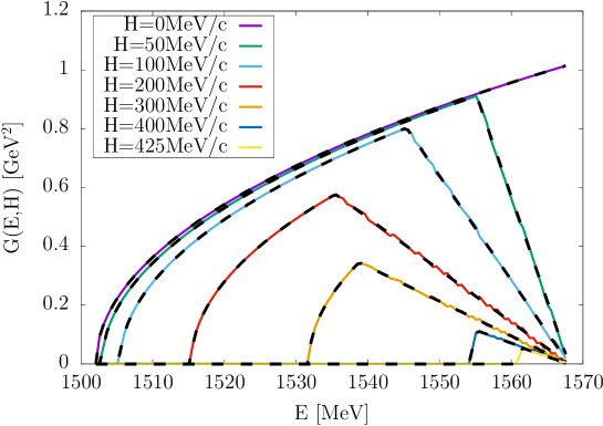
Figure 2: The integrated 2h spectral function $G(E,H)$ for various values of momentum $H$ as a function of energy $E$. The Fermi momentum is $k_{F}=225$ MeV/c. Each curve corresponds to a specific value of momentum $H$. The dashed lines represent the exact analytical result. The solid lines are numerical calculation in the center-of-mass system.

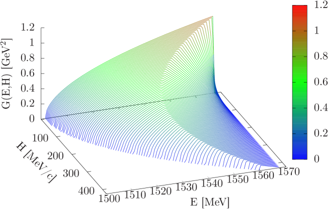
Figure 3: Three-dimensional representation of the integrated 2h spectral function $G(E,H)$. of Fig. 2

IV.1 Integrated 2h spectral function

In Fig. 2, we present the integrated spectral function $G(H,E)$ calculated using the analytical formula from Eq. (78). The results are compared to a numerical calculation in the center-of-mass (CM) frame of the two particles. $G(E,H)$ is plotted as a function of the total 2h energy $E$ for various values of $H$ ranging from zero up to close to $2k_{F}$. Note that the accessible values of $E$ lie between $E_{\min}=2m_{N}^{*}$ and $E_{\rm max}=2E_{F}$, with $E_{F}=\sqrt{k_{F}^{2}+(m_{N}^{*})^{2}}=783$ MeV. For $H=0$, all values of $E$ are allowed, and $G(E,H)$ increases continuously from zero at $E_{\min}$ to its maximum value. Indeed, for $H=0$, nucleon pairs moving back-to-back in the laboratory frame with any energy can contribute. As $H$ increases, the value of $E_{\min}$ also increases, and below this value, $G$ is zero. This means that if the nucleon pair doesn’t have a certain energy, it’s not possible for their momenta to sum up to $H$. As $H$ approaches $2k_{F}$, the spectral function is nonzero only when nucleons have energy close to the Fermi energy. For intermediate values of $H$, the function $G(E,H)$ smoothly increases with energy until it reaches a point where its derivative is discontinuous. After this point, it decreases linearly until it reaches zero at $E=2E_{F}$. The discontinuity in the derivative is due to Pauli blocking when the value of $\epsilon_{A}$ changes abruptly in Eq. (77).

In Fig. 3, a three-dimensional plot of $G(E,H)$ is presented, revealing the characteristic structure of this universal function for the Fermi gas. The function is nonzero only in regions allowed by kinematics, that is, in the phase space allowed for two holes with momentum $H$ and energy $E$. It is expected that in a more realistic model of a finite nucleus, this function would be modified and exhibit signs of a shell structure, while the maximum momentum would extend beyond $2k_{F}=450$ MeV. However, this structure is averaged out and smeared in neutrino experiments where energy transfer cannot be measured and when integrating over some of the variables of the final particles. On the other hand, the factorized approximation allows for modifying the function $G$ by replacing it with a more realistic function calculated by other methods. This is another advantage of the factorized model.

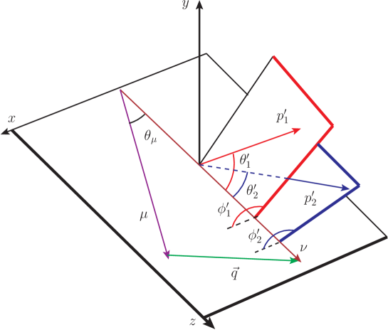
Figure 4: Coordinate system and kinematics in the semi-inclusive two-nucleon emission reaction.

IV.2 Semi-inclusive 2p2h cross section integrated over one energy

The coordinate system and kinematics for the description of semi-inclusive 2p2h is shown in Fig. 4. We choose the $z$-axis in the direction of the incident neutrino. The neutrino and the final muon directions define the scattering plane $(x,z)$ The directions of the two final momenta ${\bf p}^{\prime}_{i}$ and the $z$ axis define the two reaction planes that form angles $\phi^{\prime}_{1}$ and $\phi^{\prime}_{2}$, respectively, with the scattering plane. The angles between ${\bf p}^{\prime}_{i}$ and the $z$ axis are $\theta^{\prime}_{i}$.

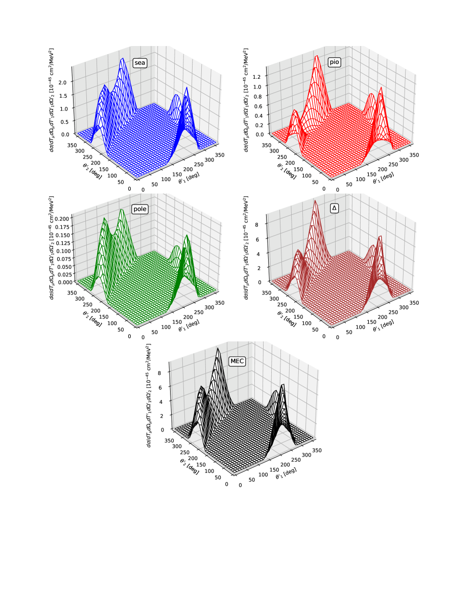
Figure 5: The sum of semi-inclusive ¹²C$(\nu_{\mu},\mu^{-}pp)$ plus ¹²C$(\nu_{\mu},\mu^{-}pn)$ cross sections computed with the factorized model for in-plane kinematics of the two final particles. Incident neutrino energy is $E_{\nu}=750$ MeV, muon energy $E_{\mu}=550$ MeV, muon angle $\theta_{\mu}=15\mbox{${}^{\rm o}$}$ and kinetic energy of the first particle (a proton) fixed to $T^{\prime}_{1}=50$ MeV. The energy of the second nucleon is integrated. In each panel one of the seagull, pionic, pole, $\Delta$, and total MEC contributions, are shown.

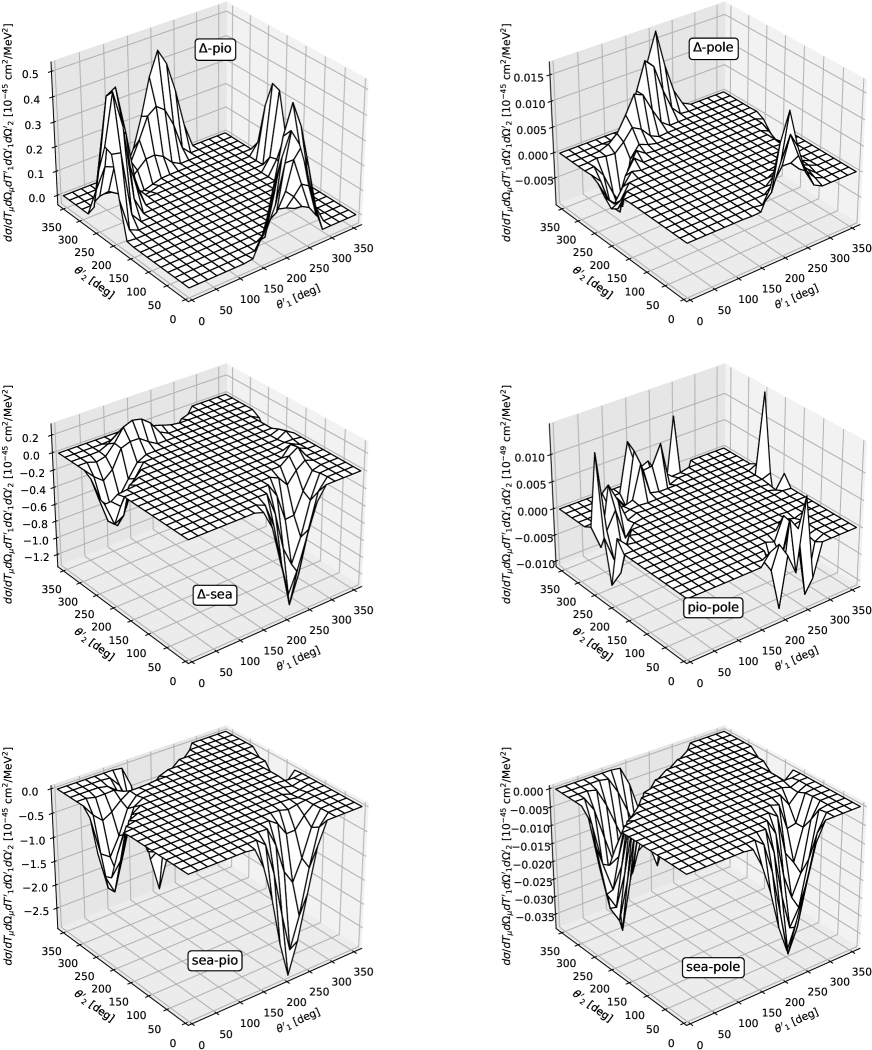
Figure 6: The same as Fig. 5 for the interferences between the different MEC contributions. Each panel of this figure show a different interference pattern corresponding to $\Delta$-pionic, $\Delta$-pole, $\Delta$-seagull, pionic-pole, seagull-pionic and seagull-pole.

In Figs. 5 and 6, results for the semi-inclusive 2p2h cross section for neutrino scattering are presented, integrated over the energy of the second nucleon and summed over pp and pn pairs.

$$\frac{d\sigma}{dT_{\mu}d\Omega_{\mu}dT^{\prime}_{1}d\Omega^{\prime}_{1}d\Omega^{\prime}_{2}}=\frac{d\sigma_{pp}}{dT_{\mu}d\Omega_{\mu}dT^{\prime}_{1}d\Omega^{\prime}_{1}d\Omega^{\prime}_{2}}+\frac{d\sigma_{pn}}{dT_{\mu}d\Omega_{\mu}dT^{\prime}_{1}d\Omega^{\prime}_{1}d\Omega^{\prime}_{2}}.$$ (80)

Thus particle 1 corresponds to a proton, and particle 2 can be a proton or neutron. The neutrino energy is fixed at $E_{\nu}=750$ MeV, muon angle $\theta_{\mu}=15$ degrees, and muon energy is 550 MeV. The kinetic energy of the first proton is fixed at $T^{\prime}_{1}=50$ MeV. The kinematics are coplanar, meaning that the two nucleons exit in the scattering plane. In Fig. 5, the cross section is plotted as a function of the angles of the two particles $(\theta^{\prime}_{1},\theta^{\prime}_{2})$, both ranging from 0 to $2\pi$. This means that we are simultaneously plotting the 4 cases $\phi^{\prime}_{1},\phi^{\prime}_{2}=0,\pi$. When $\theta^{\prime}_{i}>\pi$, the corresponding angle $\phi^{\prime}_{i}=\pi$. This case has been chosen explicitly to allow for comparison with the calculation of Van Cuyck et al. Cuy17 in the shell model, which is the only available calculation of this reaction in ¹²C.

In Fig. 5 we show the separate contributions of each of the currents: seagull, pionic, pion pole, $\Delta$, and the total, while in Fig. and 6 we present the interferences between pairs of currents. In Ref. Cuy17 , the contribution of the $\Delta$ was not computed. Comparing with Figure 4 of Ref. Cuy17 , we see that the agreement with the shell model is quite good, considering that we are using a Fermi gas and that the momentum transfer is relatively low ($q=265$ MeV/c) for this kinematics, while $\omega=200$ MeV. Since the quasielastic peak for this value of $q$ is approximately $\omega_{QE}=q^{2}/2m_{N}\simeq 37$ MeV, we are in the energy transfer region well above the quasielastic peak, close to the photon point, where the 2p2h MEC contribution is most important.

Comparing the magnitude of the separate cross sections with Fig. 4 of Ref. Cuy17 , we note that in the case of the seagull and pionic currents, our cross section is somewhat larger than in the calculations of Ref. Cuy17 . Specifically, the maxima of the seagull, pion in flight and pion pole cross section are $(\sigma_{S},\sigma_{\pi},\sigma_{P})$ $\sim(2.2,1.2,0.2)u$ in the RMF, close to the values $\sim(1.8,1,0.25)u$ obtained in the shell model, in units of $u=10^{-45}\,{\rm cm^{2}/MeV^{2}}$.

The structure of the two peaks observed in Fig. 5 is also similar to that of the shell model, with approximately the same angular positions, although in the shell model, they are apparently somewhat wider. This can be understood given that, in the finite nucleus model, the momenta are extended and are not limited above the Fermi momentum. In our case we used the factorized formula (79). This indicates that the integrated 2h spectral function captures well the momentum and energy dependence of the semi-inclusive cross section in more realistic models. Additionally, the averaged values of the hole momenta in the elementary 2p2h tensor are approximately suitable.

One reason for the agreement with the shell model is that the process is semi-inclusive and we are integrating over the energy of the second particle. In the shell model, a sum over occupied shells has been performed. The integral over energy and sum over shells produce an smearing of the 2h spectral distribution. Similarly, in the RMF, we are integrating over holes, producing a similar effect of smearing.

Another reason for the good agreement with the shell model is that we have performed the correct energy-momentum balance in the kinematics. This includes taking into account that the given kinetic energy $T^{\prime}_{1}$ in the semi-inclusive process is the asymptotic energy when the nucleon is detected. In the shell model, it is the total final energy of the particle when it is far from the nucleus, where the nuclear potential is zero. In the case of the RMF the total energy must include the vector energy. Asymptotically, this must be equal to the nucleon mass plus the asymptotic kinetic energy. Thus, the correct energy balance for the first particle is

$$E^{\prime}_{1}+E_{v}=m_{N}+T^{\prime}_{1}\Longrightarrow E^{\prime}_{1}=m_{N}+T^{\prime}_{1}-E_{v}.$$ (81)

Taking into account that $E_{v}=141$ MeV, this gives $E^{\prime}_{1}=848$ MeV. From Eq. (81) it follows that the momentum of the particle in the RMF must be computed as

$$(p^{\prime}_{1})^{2}=(m_{N}+T^{\prime}_{1}-E_{v})^{2}-(m_{N}^{*})^{2}$$ (82)

that gives $p^{\prime}_{1}=393$ MeV/c. Or, assuming non relativistic kinematics for the case of Fig. 5,

$$m_{N}^{*}+\frac{(p^{\prime}_{1})^{2}}{2m_{N}^{*}} = m_{N}+T^{\prime}_{1}-E_{v}\Longrightarrow$$

$$(p^{\prime}_{1})^{2} = 2m_{N}^{*}(m_{N}-m_{N}^{*}+T^{\prime}_{1}-E_{v})=2m_{N}^{*}(E_{s}-E_{v}+T^{\prime}_{1}),$$ (83)

with $E_{s}=m_{N}-m_{N}^{*}=188$ MeV is the (positive) scalar energy, and $E_{s}-E_{v}=47$ MeV Mar21a . This gives a momentum $p^{\prime}_{1}=381$ MeV/c.

Therefore, the differential cross section must be transformed with appropriate Jacobian. From Eq. (83), we have $p^{\prime}_{1}dp^{\prime}_{1}=m_{N}^{*}dT^{\prime}_{1}$. Hence

$$d^{3}p^{\prime}_{1}=m_{N}^{*}p^{\prime}_{1}dT^{\prime}_{1}d\Omega^{\prime}_{1}$$ (84)

and the differential cross section transforms as

$$\frac{d\sigma}{dT_{\mu}d\Omega_{\mu}dT^{\prime}_{1}d\Omega^{\prime}_{1}d\Omega^{\prime}_{2}}=m_{N}^{*}p^{\prime}_{1}\frac{d\sigma}{dT_{\mu}d\Omega_{\mu}d^{3}p^{\prime}_{1}d\Omega^{\prime}_{2}}.$$ (85)

A similar transformation can be obtained for the relativistic case of Eq. (82):

$$d^{3}p^{\prime}_{1}=E^{\prime}_{1}p^{\prime}_{1}dT^{\prime}_{1}d\Omega^{\prime}_{1}$$ (86)

and the differential cross section transforms as

$$\frac{d\sigma}{dT_{\mu}d\Omega_{\mu}dT^{\prime}_{1}d\Omega^{\prime}_{1}d\Omega^{\prime}_{2}}=E^{\prime}_{1}p^{\prime}_{1}\frac{d\sigma}{dT_{\mu}d\Omega_{\mu}d^{3}p^{\prime}_{1}d\Omega^{\prime}_{2}}.$$ (87)

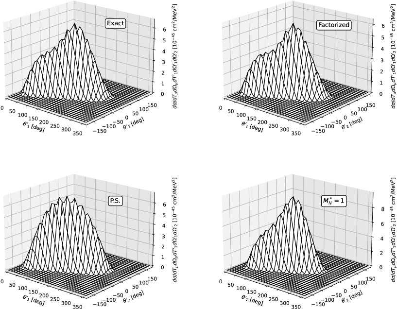
Figure 7: Similar as Fig. 5 but for $p^{\prime}_{1}=278$ MeV/c, and changing the interval of the $\theta^{\prime}_{2}$ axis from $[0,360]$ to $[-180,180]$. In each panel we show the cross section computed using a different reaction model: The exact RMF model, the factorized model, the pure phase-space model (P.S.), and the RFG model with a separation energy of 40 MeV.

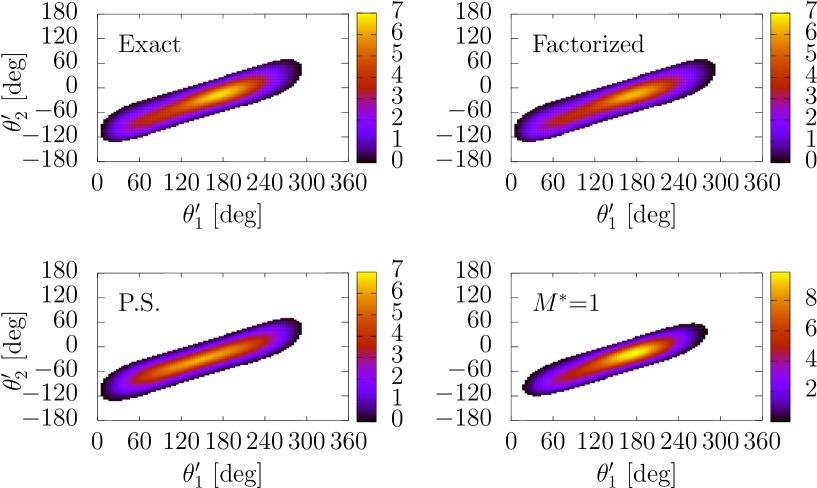
Figure 8: Color map representation of Fig.7, where the semi-inclusive cross section $d\sigma/dT_{\mu}d\Omega_{\mu}dT^{\prime}_{1}d\Omega^{\prime}_{1}d\Omega^{\prime}_{2}$ for the sum of $pp$ and $pn$ neutrino emission channels is plotted in units of $10^{-45}$ cm²/MeV².

The meticulous consideration of the correct energy-momentum balance and the appropriate transformation of the cross section, accounting for the asymptotic kinetic energy and the Jacobian factor, ensures the consistency and reliability of our results. This level of attention to the details of the theoretical framework is crucial for obtaining meaningful comparisons with other models, especially when dealing with different formalisms or experimental measurements.

The comparison between the exact semi-inclusive cross section and the factorized model is crucial for validating the latter. In Figs. 7 and 8, we present the results for the same cross section as in Figs. 5 and 6, focusing on the same kinematics, but displaying the range of the angle $\theta^{\prime}_{2}$ varying between $-180$ and $180$ degrees for better visualization, Now the cross section appears as a single peak as a function of the angles. The top panels in Figs. 7 and 8 depict the results of both the exact and factorized calculations, revealing striking similarities. The shape resembles an asymmetric peaked structure with a shoulder, slightly more pronounced in the factorized case. Besides this, there are no significant differences, and the magnitude is the same.

This contrasts with the results obtained using a pure-phase space (PS) model, shown in the bottom left panels of figs 7 and 8. The pure-phase space model assumes a constant hadronic tensor, making the results to follow the shape of the integrated 2h spectral function and normalized to the inclusive 2p2h cross section. This is analogous to the procedure employed in Monte Carlo event generators. The PS model exhibits a peak, but the position of the maximum is shifted, and the shape of the peak is more symmetric, lacking the shoulder observed in models with a hadronic tensor. This underscores the importance of considering the effect of the hadronic tensor in such reactions. Finally, in the bottom right panel, we compare the calculation with the RFG without effective mass, but with a separation energy, revealing a significant difference in magnitude compared to the RMF. Additionally, the peak is somewhat narrower in the RFG case. This emphasizes the impact of the effective mass and the necessity of considering it in the formalism.

Figure 9: Left panels: semi-inclusive pp and pn emission cross section for neutrino scattering as a function of $p^{\prime}_{2}$. In each panel A–D the lepton kinematics and angles of the exit particles are fixed to the values defined in Table 1. Right panels: the averaged elementary 2p2h hadronic tensor $\langle w^{\mu\nu}_{N_{1}N_{2}}({\bf p}^{\prime}_{1},{\bf p}^{\prime}_{2},{\bf q},\omega)\rangle$ defined in Eq. (50), compared to the elementary 2p2h hadronic tensor evaluated for averaged hole momenta $w^{\mu\nu}_{N_{1}N_{2}}({\bf p}^{\prime}_{1},{\bf p}^{\prime}_{2},\langle{\bf h}_{1}\rangle,\langle{\bf h}_{2}\rangle)$ as a function of $p^{\prime}_{2}$ for the same kinematics.

In Fig. 9, we present another test of the factorized approach compared with the exact result. In the right panels, we display the full semi-inclusive 2p2h cross section as a function of $p^{\prime}_{2}$ for the same kinematics as in Fig. 5 (panels A, B). In this case, we have fixed the four angles $\theta^{\prime}_{1},\theta^{\prime}_{2},\phi^{\prime}_{1},\phi^{\prime}_{2}$, corresponding to two representative points on the plot in Fig. 5, which are shown in Table 1. We also show the results for kinematics C and D of Table 1, corresponding to a different lepton kinematics. Kinematics C and D were used in Ref. Mar24 to compute semi-inclusive two nucleon emission integrated over four variables. In Fig. 9 we show the separate pp and pn emission channels for each one of the three models: exact, factorized, and phase-space models.

Here, it is evident that the choice of averaged values for the hole momenta in the factorized model does not differ significantly from the exact result, where the elementary 2p2h hadronic tensor is integrated over the holes. Both models exhibit very similar behavior. On the other hand, in the phase-space model, the elementary 2p2h hadronic tensor is considered a constant and is normalized to the inclusive 2p2h cross section. This leads to the shapes of the curves in the phase-space model resembling less closely the exact case, even though the order of magnitude is appropriate due to normalization.

Table 1: Kinematics used for the results of Fig. 9 of the semi-inclusive 2p2h cross section. Kinematics A and B are from Figs. 5 and 6. Kinematics C and D where also employed in Ref. Mar24 to compute the two-folded semi-inclusive cross section.

Kin.	$E_{\nu}$ [MeV]	$E_{\mu}$ [MeV]	$p^{\prime}_{1}$ [MeV/c]	$\phi_{1}$	$\phi_{2}$	$\theta_{1}$ [deg.]	$\theta_{2}$ [deg.]
A	750	550	278	0	$\pi$	172	341
B	750	550	278	0	$\pi$	140	330
C	950	600	400	$\pi$	$\pi$	250	355
D	950	600	400	0	$\pi$	50	285

In the right column of Fig. 9, we present additional results for the averaged elementary 2p2h hadronic tensor for the same kinematics, comparing it to the tensor evaluated over averaged holes. Specifically, we plot the contraction with the leptonic tensor

$$\sigma_{0}L_{\mu,\nu}\langle w^{\mu\nu}({\bf p}^{\prime}_{1},{\bf p}^{\prime}_{2},{\bf q},\omega)\rangle,$$

and compare it to the contraction with the elementary 2p2h tensor evaluated over averaged holes

$$\sigma_{0}L_{\mu,\nu}w^{\mu\nu}({\bf p}^{\prime}_{1},{\bf p}^{\prime}_{2},\langle{\bf h}_{1}\rangle,\langle{\bf h}_{2}\rangle).$$

Both pp and pn emission channels are shown in the figure. The agreement between both models is quite good, highlighting that the elementary hadronic tensor is not constant but depends on the kinematics. This dependence is clearly observed in the figure, emphasizing the need to consider the full momentum and energy dependence in the tensor, as is done in the factorized model, rather than assuming a constant value, as in the phase-space model.

Finally, in Figs. 10 and 11, we explore the semi-inclusive cross section integrated over one energy, focusing on different increasing values of the proton momentum $p^{\prime}_{1}$. In Fig. 10 the lepton kinematics is the same as in Fig. 5 and $p^{\prime}_{1}=278$, 393, and 600 MeV/c. In Fig. 11 the lepton kinematics is different with larger neutrino energy $E_{\nu}=950$ MeV, $E_{\mu}=600$ MeV, and $\cos\theta_{\mu}=0.85$. This correspond to ’Kinematic #1’ from Ref. Mar23b , where we computed the semi-inclusive cross section integrated over four variables. The three different values of proton momentum in Fig 11 are $p^{\prime}_{1}=400$ MeV/c, 600 MeV/c, and 800 MeV/c.

An important general feature that emerges from these angular distribution plots is that the two nucleons tend to be emitted in opposite directions. The back-to-back tendency is only approximate. This means that the angle between $\mathbf{p}^{\prime}_{1}$ and $\mathbf{p}^{\prime}_{2}$ is greater than 90 degrees and predominantly closer to 180 degrees. For example, in the top panels of Fig. 10, the maximum of the cross section occurs around $\theta^{\prime}_{1}\sim 200$ degrees and $\theta^{\prime}_{2}\sim 350$ degrees. That is, $\theta^{\prime}_{2}-\theta^{\prime}_{1}\sim 150$ degrees. It can also be seen in the values of Table 1, corresponding to angular positions where the cross section is significant, where the differences between the fifth and fourth columns are $\theta^{\prime}_{2}-\theta^{\prime}_{1}=169$, 190, 105, and 235 degrees. This approximate tendency of nucleons to be emitted back-to-back will also be independently confirmed by the results of the next section.

These plots provide insights into how the distributions evolve and change shape as the energy of the detected nucleon increases. The strength shifts angularly, and the main peak changes its position. In Fig. 10, as the energy increases, the shoulder observed in Fig. 7 becomes more pronounced, eventually splitting into two distinct peaks. However, for $p^{\prime}_{1}=600$ MeV/c, there is a return to a single peak but in a different angular position. Something similar happens for the kinematics of Fig. 11.

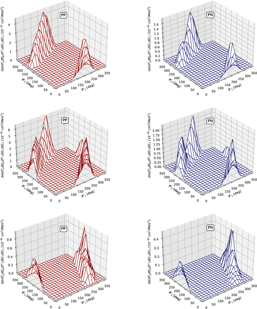
Figure 10: Semi-inclusive two-nucleon emission cross sections integrated over the second particle, for neutrino scattering and separated in proton-proton (pp) and neutron-neutron (nn) channels. The kinematics as in Fig.5 but with different values of proton momentum, $p^{\prime}_{1}=278$ MeV/c in the top panel, 393 MeV/c in the middle panel, and 600 MeV/c in the bottom panel. The pp channel is depicted in red on the left side, while the pn-channel is represented in blue on the right side.

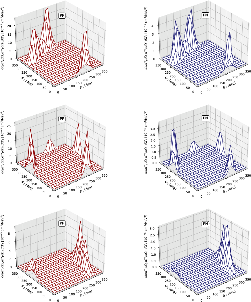
Figure 11: The same as Fig. 10 for a different kinematics given by $E_{\nu}=950$ MeV $E_{\mu}=600$ MeV and $\cos\theta_{\mu}=0.85$ (’Kinematic #1’ from Mar23b ). The panels represent three different values of proton momentum $p^{\prime}_{1}=400$ MeV/c (top panels), 600 MeV/c (middle panels), and 800 MeV/c (bottom panels).

IV.3 Semi-inclusive 2p2h cross section integrated over the muon

In this last subsection, we explore another observable of interest in semi-inclusive two-nucleon emission: the cross section integrated over the muon energy and angles, as well as the final nucleon angles.

$$\frac{d\sigma_{N_{1}N_{2}}}{dp^{\prime}_{1}dp^{\prime}_{2}}=2\pi p^{\prime}_{1}{}^{2}p^{\prime}_{2}{}^{2}\int_{T_{\rm min}}^{T_{\rm max}}dT_{\mu}\int_{u_{\rm min}}^{1}d\cos\theta_{\mu}\int d\Omega^{\prime}_{1}\int d\Omega^{\prime}_{2}\frac{d\sigma_{N_{1}N_{2}}}{dT_{\mu}d\Omega_{\mu}d^{3}p^{\prime}_{1}d^{3}p^{\prime}_{2}}$$ (88)

where the integration limits are given below.

The motivation for this study is to compare predictions with the Valencia model and recent results obtained within the NEUT generator, as published in the reference Sob20 . This comparison is valuable because the Valencia model also employs an interacting relativistic Fermi gas, introducing interaction through a different effective interaction. Additionally, it includes effects such as short-range and long-range correlations of the RPA type, while neglecting the interference of the direct and exchange current matrix elements, among other considerations detailed in Sob20 . On the other hand, results from the NEUT generator are representative of what is expected from a model that applies a phase-space approximation for the 2p2h emission, neglecting the dependence of the hadronic tensor on the exclusive variables ${\bf p}^{\prime}_{1},{\bf p}^{\prime}_{2},{\bf h}_{1},{\bf h}_{2}$. In contrast, we apply the factorized approximation of the RMF model, which has been tested in the previous subsection and yields results very similar to the shell model of Cuy17 .

The factorized approximation in this case is convenient because it saves us from the computation of an eight-dimensional integral, as required by the exact calculation. The factorization allows us to use the analytical formula for the $G(E,H)$ function, introducing the elementary 2p2h hadronic tensor evaluated at averaged hole momenta. Thus, we are left with a six-dimensional integral that needs to be computed numerically.

First we examine the integration limits that we have written explicitly in Eq. (88) for the muon kinetic energy $T_{\rm min}<T_{\mu}<T_{\rm max}$ and angle $u_{\rm min}<\cos\theta_{\mu}<1$. Note that these integration limits are specific for our RMF+MEC approach and are not general.

We maintain a fixed neutrino energy, $E_{\nu}$, while considering $p^{\prime}_{1}$ and $p^{\prime}_{2}$ as the fixed momenta of the emitted nucleons. Consequently, the energies $E^{\prime}_{1}$ and $E^{\prime}_{2}$ are also predetermined. The conservation of energy is expressed by the equation $E_{\mu}=E_{\nu}+E_{1}+E_{2}-E^{\prime}_{1}-E^{\prime}_{2}$. In our model the initial hole energies are bounded within the range $m_{N}^{*}<E_{i}<E_{F}$. This bounding of initial particle energies inherently limits the energy available for the muon, ensuring $E_{\mu}$ falls within a defined range.

$$E_{\nu}+2m_{N}^{*}-E^{\prime}_{1}-E^{\prime}_{2}<E_{\mu}<E_{\nu}+2E_{F}-E^{\prime}_{1}-E^{\prime}_{2}.$$ (89)

This means that the integration limits must be

$$T_{\rm min} = E_{\nu}-m_{\mu}+2m_{N}^{*}-E^{\prime}_{1}-E^{\prime}_{2},$$ (90)

$$T_{\rm max} = E_{\nu}-m_{\mu}+2E_{F}-E^{\prime}_{1}-E^{\prime}_{2}.$$ (91)

The lower limit of $\cos\theta_{\mu}$ for fixed $E_{\nu}$ and $E_{\mu}$ is due to the fact that the 2p2h response can be neglected if the energy transfer is below the threshold energy to kick two initially at-rest particles that are emitted with a total momentum $q$ (frozen nucleon approximation). Therefore, the dominant contribution to the integral requires that

$$E\nu-E\mu=\omega>\sqrt{4(m_{N}^{*})^{2}+q^{2}}-2m_{N}^{*}$$ (92)

From where

$$(E_{\nu}-E_{\mu}+2m_{N}^{*})^{2}\geq 4(m_{N}^{*})^{2}+q^{2}.$$ (93)

On the other hand the momentum transfer is given by

$$q^{2} = (k-k^{\prime})^{2}=k^{2}+k^{\prime 2}-2kk^{\prime}\cos\theta_{\mu}$$ (94)

$$= E_{\nu}^{2}+E_{\mu}^{2}-m_{\mu}^{2}-2E_{\nu}\sqrt{E_{\mu}^{2}-m_{\mu}^{2}}\cos\theta_{\mu}$$ (95)

Substituting this value of the momentum transfer in Eq. (93) and expanding the square,

$$E_{\nu}^{2}+E_{\mu}^{2}-2E_{\nu}E_{\mu}+4(m_{N}^{*})^{2}+4m_{N}^{*}(E\nu-E_{\mu})$$ (96)

$$\kern-142.26378pt\geq 4(m_{N}^{*})^{2}+E_{\nu}^{2}+E_{\mu}^{2}-m_{\mu}^{2}-2E_{\nu}\sqrt{E_{\mu}^{2}-m_{\mu}^{2}}\cos\theta_{\mu}.$$

Solving for $\cos\theta_{\mu}$ and simplifying we obtain the lower limit:

$$\cos\theta_{\mu}\geq\frac{2E_{\nu}E_{\mu}-m_{\mu}^{2}-4m_{N}^{*}(E_{\nu}-E_{\mu})}{2E_{\nu}\sqrt{E_{\mu}^{2}-m_{\mu}^{2}}}\equiv u_{\rm min}$$ (97)

Applying these integration limits when performing the numerical integral helps speed up the calculation, as it avoids calculating the 2p2h hadronic tensor for kinematics that are suppressed by these limits.

The integrated cross section from Eq. (88) is shown in figures 12 for neutrinos and 13 for antineutrinos. We present the results for three incident neutrino energies: $E_{\nu}=500$, 1000, and 1500 MeV. These values are the same as those used in figures 11 and 12 of ref. Sob20 for neutrino scattering, considering the same observable for comparison. In our results, we employ two models. One is the pure phase space (top panels of Fig. 12, 13), where the elementary 2p2h hadronic tensor is not included. Specifically, in the P.S. model, we set $L_{\mu\nu}w^{\mu\nu}({\bf p}^{\prime}_{1},{\bf p}^{\prime}_{2},{\bf h}_{1},{\bf h}_{2})=1$. Therefore, the model only contains the integrated 2h spectral function, and it is normalized with a constant so that the PS total cross section coincides with the factorized one. We present these results as a way to observe the effect of the elementary 2p2h tensor hadronic in this observable. The other calculations shown in the middle and bottom panels of Fig. 11 correspond to the emission channels of pp and pn, respectively. In these cases, the first particle, $p^{\prime}_{1}$, is always a proton, while $p^{\prime}_{2}$ can be either a proton or a neutron.

The first thing we notice is the shape of the distribution in the plane $(p^{\prime}_{1},p^{\prime}_{2})$. The cross section is zero beyond an a surface that is approximately a quarter of a circle centered at the point $(p^{\prime}_{1},p^{\prime}_{2})=(k_{F},k_{F})$, because $k_{F}$ is the minimum value of $p^{\prime}_{i}$. The boundary of the surface is determined by energy conservation. The curve defining the boundary of the surface can be written as a function of $p^{\prime}_{2}$ in terms of $p^{\prime}_{1}$. In fact, we use energy conservation

$$E^{\prime}_{1}+E^{\prime}_{2}=E_{\nu}-E_{\mu}+E_{1}+E_{2}$$ (98)

and apply that the maximum energy of the holes is the Fermi energy, and the minimum energy of the muon is the muon mass:

$$E_{1}+E_{2}<2E_{F}$$ (99)

$$m_{\mu}<E_{\mu}\Longrightarrow-E_{\nu}<-m_{\mu}$$ (100)

Then we have

$$E^{\prime}_{1}+E^{\prime}_{2}<E_{\nu}-m_{\mu}+2E_{F}\Longrightarrow E^{\prime}_{2}<E_{\nu}-m_{\mu}+2E_{F}-E^{\prime}_{1}.$$ (101)

Taking the square of the last inequality and solving for the momentum, we obtain the limiting curve

$$p^{\prime}_{2}<p^{\prime}_{2}{}_{\rm max}=\sqrt{\left(E_{\nu}-m_{\mu}+2E_{F}-\sqrt{p_{1}^{{}^{\prime}2}+(m_{N}^{*})^{2}}\right)^{2}-(m_{N}^{*})^{2}}$$ (102)

The curve $p^{\prime}_{2}{}_{\rm max}$ as a function of $p^{\prime}_{1}$ is plotted in Fig. 14 for several values of the neutrino energy. Comparing with Figs. 12 and 13 we see that they explain the border of the distribution.

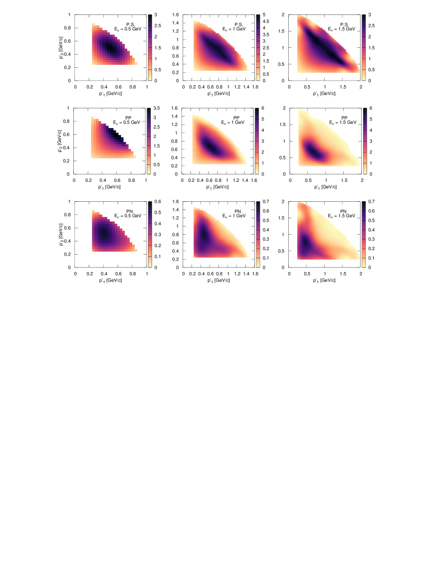
Figure 12: Integrated semi-inclusive cross section $d\sigma_{N_{1}N_{2}}/dp^{\prime}_{1}dp^{\prime}_{2}$ as a function of outgoing nucleon momenta for three neutrino energies: $E_{\nu}=500$ MeV, 1000 MeV, and 1500 MeV. In the top panels we show the pure phase-space (P.S.) results. In the middle and bottom panels we show the pp and pn emission channels, respectively, computed with the factorized RMF model. The phase space is normalized to the inclusive total neutrino cross section. The units are $10^{-38}$ cm²/GeV².

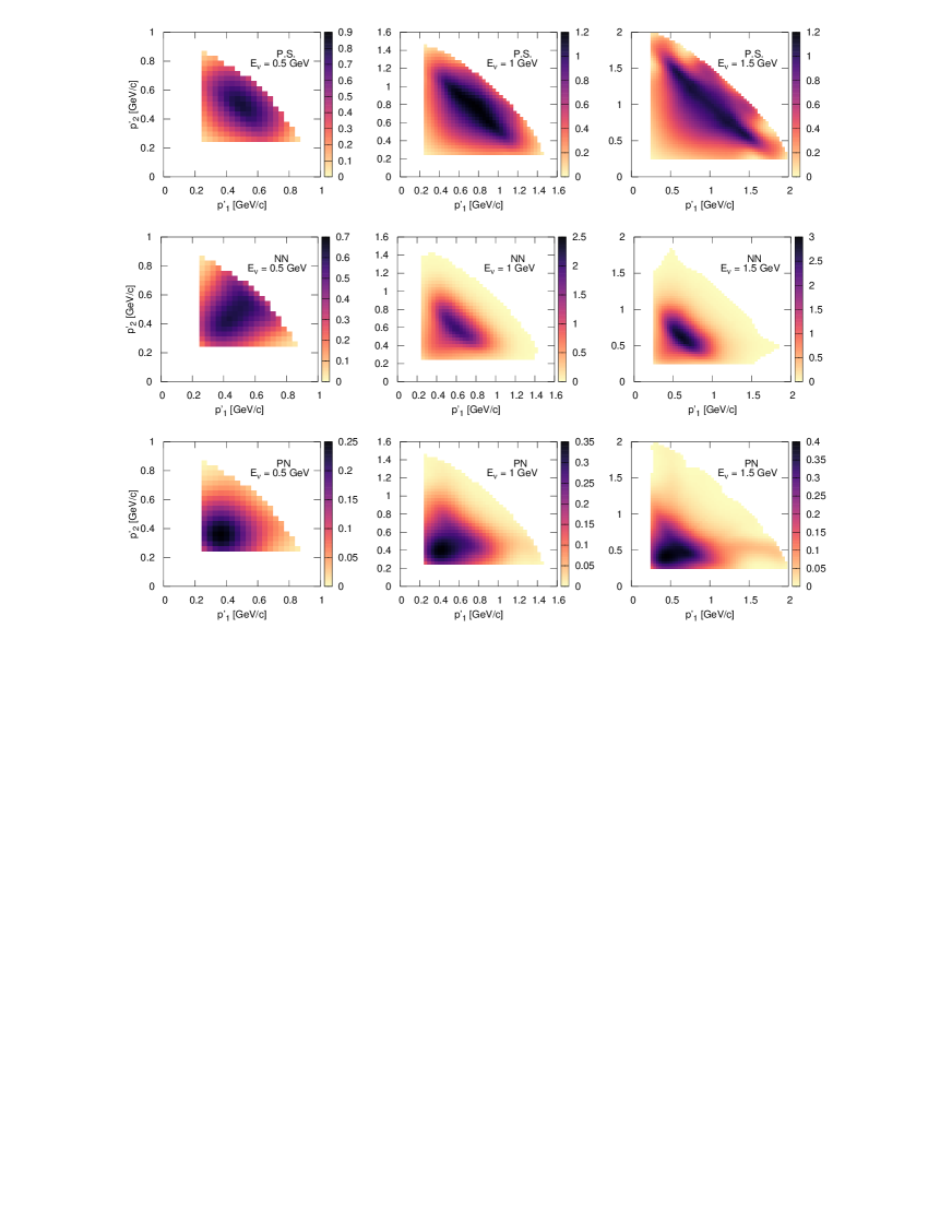
Figure 13: The same as Fig. 12 for antineutrino scattering.

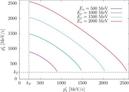
Figure 14: Maximum values of outgoing nucleon momentum $p^{\prime}_{2}$ as a function of $p^{\prime}_{1}$ for various neutrino energies

The second observation from figs. 12 and 13 is that the peak of the distribution in the case of the phase-space model (PS) shifts towards larger momenta as the neutrino energy increases. However, in the case of the factorized model, the peak remains more or less in the same position in the $(p^{\prime}_{1},p^{\prime}_{2})$ plane, both in pp and pn emission. This is due to the inclusion of the elementary 2p2h hadronic tensor, which has a peak around the $\Delta$ resonance. The results in the figure show that the position of this peak does not change much with increasing neutrino energy.

A possible explanation of the invariance of the position of the distribution peak is based on the assumption of back-to-back dominance of the final particles, as we have seen in the angular distributions of the last section, together with the additional assumption of dominance of the $\Delta$-forward diagrams of the MEC for pp emission. In fact the argument is the following. To simplify this discussion we set the effective mass equal to the nucleon mass. The assumption is that the greatest contribution to the cross section comes from back-to-back nucleons. From momentum conservation this gives

$${\bf q}+{\bf h}_{1}+{\bf h}_{2}={\bf p}^{\prime}_{1}+{\bf p}^{\prime}_{2}\simeq 0\Longrightarrow{\bf q}+{\bf h}_{1}\simeq-{\bf h}_{2}.$$ (103)

Assuming the dominance of the $\Delta$-forward current, if the first nucleon absorbs the energy-momentum transfer (diagram (f) of Fig. 1), then the maximum contribution occurs when the $\Delta$ propagator is at its maximum, i.e., we are close to an on-shell $\Delta$:

$$(\omega+E_{1})^{2}-({\bf q}+{\bf h}_{1})^{2}\simeq M_{\Delta}^{2}.$$ (104)

Using the result from the back-to-back condition (103) we obtain

$$\omega+E_{1}\simeq\sqrt{h_{2}^{2}+M_{\Delta}^{2}}.$$ (105)

Using this result in the energy conservation

$$2E^{\prime}_{1}\simeq E^{\prime}_{1}+E^{\prime}_{2}=\omega+E_{1}+E_{2}\simeq\sqrt{h_{2}^{2}+M_{\Delta}^{2}}+E_{2}.$$ (106)

Finally we obtain

$$E^{\prime}_{1}\simeq\frac{1}{2}\left(\sqrt{h_{2}^{2}+M_{\Delta}^{2}}+E_{2}\right).$$ (107)

This suggests that the position of the maximum contribution does not depend strongly on the energy of the incoming neutrino, as long as we are in the back-to-back configuration and the $\Delta$-forward current dominates. This could explain the observed behavior in the pp distributions of Fig. 12, where the position of the peak remains relatively stable even with increasing neutrino energy.

If we give values to the hole momentum $h_{1}=0,k_{F}$ we obtain

$$h_{1}=0 \Rightarrow E^{\prime}_{1}\simeq\frac{1}{2}(M_{\Delta}+m_{N})=1086\,{\rm MeV}\Longrightarrow p^{\prime}_{1}\simeq 546\,{\rm MeV/c}$$ (108)

$$h_{1}=k_{F} \Rightarrow E^{\prime}_{1}\simeq\frac{1}{2}\left(\sqrt{k_{F}^{2}+M_{\Delta}^{2}}+E_{F}\right)=1108\,{\rm MeV}\Longrightarrow p^{\prime}_{1}\simeq 588\,{\rm MeV/c}$$ (109)

The values obtained under our assumption, $p^{\prime}_{1}=546-588$, are not very far from the actual position of the peak in Fig. 12, $p^{\prime}_{1}\simeq 600-700$. We attribute the difference to the approximations made to obtain the rough estimation of the maximum since the nucleons do not strictly emerge back-to-back. Other contributions in the MEC, the neglect of the effective mass effect, and additional factors also contribute to the discrepancy. However, the result is reasonably sound, allowing us to suggest that the hypothesis of back-to-back dominance has some relevance to the results in Fig. 12.

The results of Fig. 12 can be compared with those of Figs 11 and 12 of Ref. Sob20 , where the same cross sections were computed for the same kinematics for pp and pn emission with the Valencia model of 2p2h emission and the NEUT event generator, which includes the final state interaction (FSI) with an intranuclear cascade model. Note that our results are directly the results of the primary vertex of the interaction and do not include FSI, which is expected to change the distribution slightly and possibly make the peak narrower.

Differences are observed between our results and those of the Valencia model. For example, the Valencia model predicted a maximum of the pp distribution for $p^{\prime}_{1}\sim 0.9-1.2$ GeV/c and $p^{\prime}_{2}\sim 0.4-0.5$ GeV/c, attributed in Ref. Sob20 to the $\Delta$ current, whereas in our case, as mentioned above, the peak is observed at $p^{\prime}_{1}=p^{\prime}_{2}\sim 0.6-0.7$ GeV/c.

The comparison with NEUT also does not agree with our pure phase space calculation, presumably because we do not normalize for each value of $q,\omega$, but to the total result of pp + pn emission. In this way, it is seen that it is important to include at least the inclusive responses as a function of $q,\omega$ to obtain some structure apart from the pure spectral function.

In the case of pn emission, another discrepancy is observed when comparing with the Valencia model. Both distributions are asymmetric when changing from proton to neutron. However, in our case, it is observed that at the maximum, the neutron exits with more energy than the proton, while the opposite occurs with the Valencia model.

An explanation for our result that the neutron is more energetic than the proton in pn emission can be made similarly to that given in Ref. Sob20 . However, in our case, where we only include MEC, the same deduction leads us to the conclusion that the neutron predominantly exits with more energy than the proton. Since the explanation in Ref. Sob20 is not detailed, we cannot draw strong conclusions about the differences. Therefore, we provide a more in-depth explanation of our results.

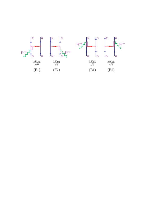
Figure 15: Feynman diagrams representing the matrix elements for forward ($K_{F1}$, $K_{F2}$) and backward ($K_{B1}$ and $K_{B2}$) $\Delta$ current for pn emission.

The argument is based on the assumption that the Delta current is the main contribution to the cross section. Under this hypothesis we compute the matrix element of the $\Delta$ current between the initial nn and final pn pair. From Eqs. (110) and (111) the $\Delta$ matrix elements are

$$j^{\mu}_{\Delta F} = \langle pn|\frac{1}{\sqrt{6}}\left[2\tau_{+}^{(2)}K_{F1}^{\mu}+2\tau_{+}^{(1)}K_{F2}^{\mu}-I_{V+}(K_{F1}-K_{F2})^{\mu}\right]|nn\rangle,$$ (110)

$$j^{\mu}_{\Delta B} = \langle pn|\frac{1}{\sqrt{6}}\left[2\tau_{+}^{(2)}K_{B1}^{\mu}+2\tau_{+}^{(1)}K_{B2}^{\mu}+I_{V+}(K_{B1}-K_{B2})^{\mu}\right]|nn\rangle,$$ (111)

Using the basic matrix elements of the isospin operators (15)

$$\langle pn|I_{V+}|nn\rangle = -2,$$ (112)

$$\langle pn|\tau_{+}^{(1)}|nn\rangle = 2,$$ (113)

$$\langle pn|\tau_{+}^{(2)}|nn\rangle = 0.$$ (114)

we obtain

$$j^{\mu}_{\Delta F} = \frac{2}{\sqrt{6}}\left(K_{F1}^{\mu}+K_{F2}^{\mu}\right)$$ (115)

$$j^{\mu}_{\Delta B} = \frac{2}{\sqrt{6}}\left(3K_{B2}^{\mu}-K_{B1}^{\mu}\right).$$ (116)

Here the functions $K_{F1}^{\mu}$, $K_{F2}^{\mu}$, $K_{B1}^{\mu}$ and $K_{B2}^{\mu}$ correspond to the diagrams of Fig. 15. It is fundamental to remember that we are considering the case where particle $p^{\prime}_{1}$ is a proton and particle $p^{\prime}_{2}$ is a neutron, as specified in fig. 15. The argument applies similarly when considering a neutron as particle 1 and a proton as particle 2, obtaining the same results.

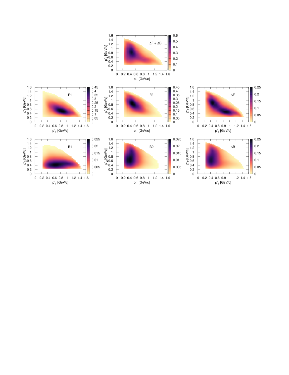
Figure 16: Color map of the cross section for neutrino-induced $pn$ emission. We display the separate contributions of the forward, $K_{F1}$, $K_{F2}$, and backward, $K_{B1}$, $K_{B2}$ terms of the $\Delta$ current, as well as the total contribution of the forward and backward, and finally the total contribution of the $\Delta$ current alone. The neutrino energy is $E_{\nu}=1$ GeV. The units of the cross section are the same as in Fig. 12

From Fig. 15 and Eqs. (115,116), it is evident that there are four main contributions to the cross section. The interaction with the initial nn pair result in a particle-hole excitation connected to the $W^{+}$, with the final particle being a proton (diagrams F1 and B1) or a neutron (diagrams F2 and B2). In the case of F1, the final proton receives a significantly higher energy-momentum transfer, while in the case of F2, the neutron becomes much more energetic. These two possible contributions have equal strength. The same can be said for backward diagrams B1 and B2.

Fig. 16 illustrates the single contributions of $K_{F1}$, $K_{F2}$, $K_{B1}$ and $K_{B2}$ to the cross section, along with the total forward and backward contribution.

We observe that the cross section obtained with the term F1 alone results in a distribution where the proton (particle 1) is more energetic than the neutron (particle 2) at the maximum. On the contrary, the contribution of the term F2 is exactly the same as F1, changing the proton for the neutron. As a result, the combined contribution of the two terms F1 + F2 produces two maxima approximately corresponding to the positions of the maxima of F1 and F2 (note that in the total result there is an interference of F1 with F2 that is also taken into account).

We now examine the individual contribution of the backward terms B1 and B2. The contribution of the term B2 has been calculated using the current $j_{B}=\frac{2}{\sqrt{6}}K_{B2}$ without the factor of 3 in Eq. (116), so that both terms enter with the same weight. Then, in Fig. 16, we see again that protons have more energy in the distribution B1, while neutrons are the most energetic in the case of B2. Again, the two distributions, B1 and B2, are obtained from each other by changing the proton for the neutron. However, in the total distribution B1 + B2, the term B2 carries a factor of 3 with respect to B1. Note that the currents are squared, meaning that the term B2 contributes actually with a factor of 9 with respect to B1. This results in the total backward distribution predominantly showing more energetic neutrons.

From these results, it also emerges that the interference between F1 and F2 is destructive since the total cross section is smaller than the individual cross sections. This makes the backward term dominate, resulting in the final observation that neutrons are more energetic when all four contributions are summed, taking into account the interferences.

As this detailed analysis shows, the comparison with other models, such as the Valencia model, should consider the distinct physics assumptions and modeling choices inherent to each approach. The differences observed underscore the complexity of the underlying nuclear dynamics and the importance of refining theoretical models to capture the intricacies of neutrino-nucleus interactions.

Finally, it is important to emphasize that this last discussion does not contradict the analysis performed to derive Eq. (107), which was based on the dominance of the $\Delta$ forward process in pp emission. The case of pp emission differs significantly from pn emission, and the various contributions enter into a different combination due to isospin considerations. On the other hand, these arguments cannot be directly applied to the case of antineutrinos in Fig. 13, where the pn distribution appears to be fairly symmetric. This symmetry in the antineutrino case arises from the subtraction of transverse terms in the hadronic tensor due to the negative sign in Eq. (3) when contracting the leptonic tensor. Therefore, careful consideration is needed when assessing the importance of different terms, as it is less straightforward and may depend on the specific kinematics involved.

V Conclusions

We have explored the semi-inclusive two-nucleon emission reaction induced by neutrinos and antineutrinos within the framework of the relativistic mean field of nuclear matter. Our approach involves a factorization approximation, where the reaction is described by an elementary two-nucleon cross section multiplied by an integrated two-hole spectral function. The 2p2h excitations are modeled using a relativistic treatment of meson-exchange currents.

One notable contribution of this work is the derivation of a simple analytical formula for the integrated two-hole spectral function. This formula not only streamlines the calculation of the cross section in the factorized case but also facilitates a clear interpretation of the obtained results. To validate the factorized approximation, we have performed comparisons with exact results obtained through numerical integration over the angles of one hole in the center-of-mass system of the two holes.

Our study has also provided a reliable prescription for the elementary two-nucleon hadronic tensor. This was achieved by evaluating the tensor at averaged hole momenta that satisfy energy-momentum conservation. These averaged momenta are chosen to be perpendicular to the missing momentum in the center-of-mass system of the two holes, as well as perpendicular to the momentum transfer. This prescription ensures a consistent treatment of the elementary two-nucleon process within the factorized model.

Our results demonstrate the efficacy of the factorized model in capturing essential features of the semi-inclusive cross section, particularly when considering the angular dependence of the two-nucleon emission. The semi-inclusive two-nucleon emission results, integrated over the energy of one of the particles, exhibit a remarkable agreement with shell model calculations of Ref. Cuy17 . This agreement is noteworthy, especially considering the Fermi gas nature of our approach. We attribute this success to the integration over holes in our model, contrasting with shell models that sum over occupied states, leading to a similar smearing effect. The correct energy balance, incorporating the effective mass and vector energy within the relativistic mean field (RMF), further contributes to the agreement. Our results also show the dominance of final state configurations close to back-to-back nucleons, i.e., the angle between is larger to 90 degrees. A comparison with a pure phase-space model reveals clear differences in the final particle distributions, underscoring the importance of considering the dependence of the hadronic tensor on the 2p2h momenta in such reactions.

Additionally, we have computed the cross section for neutrinos and antineutrinos, integrated over the muon kinematics and nucleon angles, as functions of the outgoing momenta $p^{\prime}_{1}$ and $p^{\prime}_{2}$. The factorized model significantly simplifies the computational effort, yielding smooth and distinct distributions. Our analysis of the emission distributions for pp and pn pairs has been interpreted in light of the dominance of the $\Delta$ current. Comparisons with the Valencia model reveal clear disparities, highlighting the impact of different model ingredients on the results. These differences underscore the importance of a detailed understanding of the underlying physics in neutrino-induced reactions.

This work lays the foundation for future developments that can enhance our understanding of two-nucleon emission reactions induced by neutrinos. One avenue for improvement is the incorporation of short-range correlations, considering that the two initial nucleons are correlated. A possible approach is to solve the Bethe-Goldstone equation for the initial state of the two nucleons Cas23b , revealing high-momentum components that facilitate the emission of two nucleons Mar23a . This, in conjunction with the meson-exchange current (MEC) model, would introduce an interference between short-range correlations and MEC, adding further complexity and richness to the reaction dynamics.

In this study, we have neglected the interaction in the final state. Future work could explore the inclusion of final-state interactions, providing a more comprehensive description of the entire reaction process. Another avenue for future research is to incorporate realistic two-hole spectral functions, akin to those found in the literature Geu96 ; Ben99 . This would refine the model with a more realistic distribution, and allow for a more detailed comparison with experimental data.

In summary, the factorized model developed in this work serves as a versatile tool for investigating semi-inclusive two-nucleon emission reactions in neutrino and antineutrino interactions. The insights gained from this study open up avenues for extending the model to include more sophisticated physics, such as short-range correlations and realistic spectral functions, to provide a more accurate representation of the underlying nuclear dynamics. These advancements will contribute to the ongoing efforts to unravel the intricacies of neutrino-induced reactions on nuclear targets.

Appendix A Calculation of the semi-inclusive 2p2h hadronic tensor in the center of mass system of the two holes

In this appendix we reduce an integral of the kind

$$I({\bf H},E)\equiv\int\frac{d^{3}h_{1}}{2E_{1}}\frac{d^{3}h_{2}}{2E_{2}}f({\bf h}_{1},{\bf h}_{2})\delta(E_{1}+E_{2}-E)\delta({\bf h}_{1}+{\bf h}_{2}-{\bf H})$$ (117)

to an integral over the relative angles of ${\bf h}_{1}$ in the CM system of the two holes with momenta ${\bf h}_{1},{\bf h}_{2}$ and mass $m$. Here $f({\bf h}_{1},{\bf h}_{2})$ is an arbitrary function.

We proceed in several steps:

1. First we prove the inequality

   $$m^{2}\leq E_{1}E_{2}-{\bf h}_{1}\cdot{\bf h}_{2}.$$ (118)

   In fact,

   $$0\leq({\bf h}_{1}-{\bf h}_{2})^{2}=h_{1}^{2}+h_{2}^{2}-2{\bf h}_{1}\cdot{\bf h}_{2}\Longrightarrow 2{\bf h}_{1}\cdot{\bf h}_{2}\leq h_{1}^{2}+h_{2}^{2}.$$ (119)

   On the other hand we have

   $$({\bf h}_{1}\cdot{\bf h}_{2})^{2}\leq h_{1}^{2}h_{2}^{2}.$$ (120)

   Combining (140) and (120),

   $$({\bf h}_{1}\cdot{\bf h}_{2})^{2}+2({\bf h}_{1}\cdot{\bf h}_{2})m^{2} \leq h_{1}^{2}h_{2}^{2}+(h_{1}^{2}+h_{2}^{2})m^{2}\Longrightarrow$$

   $$({\bf h}_{1}\cdot{\bf h}_{2})^{2}+2({\bf h}_{1}\cdot{\bf h}_{2})m^{2}+m^{4} \leq h_{1}^{2}h_{2}^{2}+(h_{1}^{2}+h_{2}^{2})m^{2}+m^{4}\Longrightarrow$$

   $$({\bf h}_{1}\cdot{\bf h}_{2}+m^{2})^{2} \leq (h_{1}^{2}+m^{2})(h_{2}^{2}+m^{2})=E_{1}^{2}E_{2}^{2}\Longrightarrow$$

   $${\bf h}_{1}\cdot{\bf h}_{2}+m^{2} \leq E_{1}E_{2}.$$ (121)

   This concludes the proof of (118).

2. If $E^{2}-H^{2}<4m^{2}$, then $I({\bf H},E)=0$.

   In fact we note that the product of delta functions inside the integral (117) is zero unless

   $${\bf h}_{1}+{\bf h}_{2}={\bf H},\kern 56.9055ptE_{1}+E_{2}=E.$$ (122)

   This implies that

   $$E^{2}-H^{2}=2m^{2}+2E_{1}E_{2}-2{\bf h}_{1}\cdot{\bf h}_{2}>4m^{2}.$$ (123)

   The last inequality follows from Eq. (118). Conversely, if this inequality is not satisfied, then the integral (117) is zero.

3. From step #2 above, the integral (117) can be equivalently expressed as

   $$I({\bf H},E)=\int\frac{d^{3}h_{1}}{2E_{1}}\frac{d^{3}h_{2}}{2E_{2}}f({\bf h}_{1},{\bf h}_{2})\delta(E_{1}+E_{2}-E)\delta({\bf h}_{1}+{\bf h}_{2}-{\bf H})\theta(E^{2}-H^{2}-4m^{2})$$ (124)

4. The integral $I({\bf H},E)$ can be written in the equivalent form

   $$I({\bf H},E) = \int d^{4}h_{1}d^{4}h_{2}\delta^{4}(h_{1}^{\mu}+h_{2}^{\mu}-H^{\mu})f({\bf h}_{1},{\bf h}_{2})$$ (125)

   $$\mbox{}\times\delta(h_{1\mu}h_{1}^{\mu}-m^{2})\theta(h_{1}^{0})\delta(h_{2\mu}h_{2}^{\mu}-m^{2})\theta(h_{2}^{0})\theta(E^{2}-H^{2}-4m^{2})$$

   where we have introduced the four-vectors $h_{1}^{\mu}=(h_{1}^{0},{\bf h}_{1})$, $h_{2}^{\mu}=(h_{2}^{0},{\bf h}_{2})$, and $H^{\mu}=(E,{\bf H})$.

   To prove the formula, we just need to use the following result from special relativity:

   $$\int\frac{d^{3}h_{1}}{2E_{1}}g(E_{1},{\bf h}_{1})=\int d^{4}h_{1}g(h_{1}^{\mu})\delta(h_{1\mu}h_{1}^{\mu}-m^{2})\theta(h_{1}^{0}),$$ (126)

   where $g(E_{1},{\bf h}_{1})$ is an arbitrary function.

5. We perform the integral in the CM system of the two-holes that moves with momentum ${\bf H}$. We change variables:

   $$h_{1}^{\mu}=\Lambda^{\mu}{}_{\nu}h^{\prime\prime}_{1}{}^{\nu},\kern 28.45274pth_{2}^{\mu}=\Lambda^{\mu}{}_{\nu}h^{\prime\prime}_{2}{}^{\nu},\kern 28.45274pt$$ (127)

   where $\Lambda$ is a boost transformation matrix. Double primed variables refer to the CM system. It is defined so that the coordinates of the four vector $H^{\mu}$ in the moving system are

   $${\bf H}^{\prime\prime}=0,\kern 56.9055ptE^{\prime\prime}=\sqrt{E^{2}-H^{2}}.$$ (128)

   Thus the CM system moves with velocity ${\bf v}={\bf H}/E$. In fact the new component of $H^{\mu}$ in the direction of ${\bf v}$ is given by the two-dimensional Lorentz transformation

   $$H^{\prime\prime}=\gamma(H-vE),\kern 56.9055pt\gamma=1/\sqrt{1-v^{2}},$$ (129)

   but $H^{\prime\prime}=0$ implies $v=H/E$. Note that the result of Eq. (123) implies $v<1$, so the boost is always possible.

6. Since $\det\Lambda^{\mu}{}_{\nu}=1$ we have

   $$\delta^{4}(h_{1}^{\mu}+h_{2}^{\mu}-H^{\mu})=\delta^{4}(\Lambda^{\mu}{}_{\nu}(h^{\prime\prime}_{1}{}^{\nu}+h^{\prime\prime}_{2}{}^{\nu}-H^{\prime\prime}{}^{\nu}))=\delta^{4}(h^{\prime\prime}_{1}{}^{\mu}+h^{\prime\prime}_{2}{}^{\mu}-H^{\prime\prime}{}^{\mu}).$$ (130)

   Then we can write the integral (125) in the CM system and using again Eq. (126) we arrive to the result

   $$I({\bf H},E)\equiv\int\frac{d^{3}h^{\prime\prime}_{1}}{2E^{\prime\prime}_{1}}\frac{d^{3}h^{\prime\prime}_{2}}{2E^{\prime\prime}_{2}}f({\bf h}_{1},{\bf h}_{2})\delta(E^{\prime\prime}_{1}+E^{\prime\prime}_{2}-E^{\prime\prime})\delta({\bf h}^{\prime\prime}_{1}+{\bf h}^{\prime\prime}_{2})\theta(E^{2}-H^{2}-4m^{2})$$ (131)

   Integrating over ${\bf h}_{2}^{\prime\prime}$ we have ${\bf h}_{2}^{\prime\prime}=-{\bf h}_{1}^{\prime\prime}$ and $E^{\prime\prime}_{2}=E^{\prime\prime}_{1}$. Therefore

   $$I({\bf H},E)\equiv\int\frac{d^{3}h^{\prime\prime}_{1}}{4(E^{\prime\prime}_{1})^{2}}f({\bf h}_{1},{\bf h}_{2})\delta(2E^{\prime\prime}_{1}-E^{\prime\prime})\theta(E^{2}-H^{2}-4m^{2})$$ (132)

7. To finish we integrate over the energy $E^{\prime\prime}_{1}$ using

   $$E_{1}^{\prime\prime}dE_{1}^{\prime\prime}=h_{1}^{\prime\prime}dh_{1}^{\prime\prime} \Longrightarrow d^{3}h_{1}^{\prime\prime}=h_{1}^{\prime\prime}E_{1}^{\prime\prime}dE_{1}^{\prime\prime}d\Omega_{1}^{\prime\prime},$$ (133)

   $$\delta(2E^{\prime\prime}_{1}-E^{\prime\prime}) = \frac{1}{2}\delta(E^{\prime\prime}_{1}-\frac{E^{\prime\prime}}{2}),$$ (134)

   we obtain the result $E^{\prime\prime}_{1}=E^{\prime\prime}/2$ and

   $$I({\bf H},E)=\frac{1}{4}\theta(E^{2}-H^{2}-4m^{2})\frac{h_{1}^{\prime\prime}}{2E_{1}^{\prime\prime}}\int d\Omega^{\prime\prime}_{1}f({\bf h}_{1},{\bf h}_{2})$$ (135)

   where $d\Omega_{1}^{\prime\prime}=d\cos\theta_{1}^{\prime\prime}d\phi_{1}^{\prime\prime}$ and $(\theta^{\prime\prime}_{1},\phi^{\prime\prime}_{1})$ are the angles of ${\bf h}^{\prime\prime}_{1}$ in spherical coordinates.

Appendix B Integration Limits of $G(E,H)$

In this appendix, we obtain the integration limits of the function $G(E,H)$ given by Eq. (72), as an integral over the energy $E_{1}$ of the first hole.

$$G(E,H)=\frac{2\pi(m_{N}^{*})^{2}}{H}\int_{m_{N}^{*}}^{E_{F}}dE_{1}\theta(E-E_{1}-E_{H-h_{1}})\theta(E_{H+h_{1}}-E+E_{1})\theta(E_{F}-E+E_{1}).$$ (136)

$E_{1}$ is subjected to the following conditions imposed by the step functions inside the integral

$$E_{H-h_{1}}<E-E_{1} < E_{H+h_{1}},$$ (137)

$$E-E_{1} < E_{F}.$$ (138)

By squaring the first inequality (137) and rearranging terms,

$$(m_{N}^{*})^{2}+(H-h_{1})^{2}<(E-E_{1})^{2}<(m_{N}^{*})^{2}+(H+h_{1})^{2}\Longrightarrow$$

$$H^{2}-2Hh_{1}<E^{2}-2EE_{1}<H^{2}+2Hh_{1}\Longrightarrow$$

$$-2Hh_{1}<E^{2}-2EE_{1}-H^{2}<2Hh_{1}.$$ (139)

Therefore

$$|E^{2}-H^{2}-2EE_{1}|<2Hh_{1}.$$ (140)

Note that $h_{1}$ also depends on the integration variable $E_{1}$ so we need to manipulate the inequality 140 to obtain a condition involving only $E_{1}$. It is convenient to rewrite the previous equation in terms of the dimensionless variables normalized with the nucleon mass as defined in equations (73,74), we have:

$$|\tau+\lambda\epsilon|<\kappa\eta\\$$

The next step is to take the square of this inequality, and using $\eta^{2}=\epsilon^{2}-1$ and $\kappa^{2}-\lambda^{2}=\tau$

$$\tau^{2}+\lambda^{2}\epsilon^{2}+2\tau\lambda\epsilon<\kappa^{2}\eta^{2}=\kappa^{2}(\epsilon^{2}-1)\Rightarrow$$

$$\tau^{2}+2\tau\lambda\epsilon<(\kappa^{2}-\lambda^{2})\epsilon^{2}-\kappa^{2}=\tau\epsilon^{2}-\kappa^{2}.$$ (141)

Moving the terms that depend on $\epsilon$ to the right-hand side of the inequality.

$$\tau^{2}+\kappa^{2} < \tau(\epsilon^{2}-2\lambda\epsilon)$$ (142)

$$= \tau[(\epsilon-\lambda)^{2}-\lambda^{2}]$$

$$= \tau[(\epsilon-\lambda)^{2}-\kappa^{2}+\tau]$$

$$= \tau(\epsilon-\lambda)^{2}-\tau\kappa^{2}+\tau^{2}.$$

Therefore we can write

$$\kappa^{2}(1+\tau)<\tau(\epsilon-\lambda)^{2}$$ (143)

Finally, we divide by the variable $\tau$, taking into account that $\tau<0$,

$$(\epsilon-\lambda)^{2} < \kappa^{2}\left(1+\frac{1}{\tau}\right)\Longrightarrow$$

$$|\epsilon-\lambda| < \kappa\sqrt{1+\frac{1}{\tau}}.$$ (144)

This implies that $\epsilon$ is in the interval

$$\lambda-\kappa\sqrt{1+\frac{1}{\tau}}<\epsilon<\lambda+\kappa\sqrt{1+\frac{1}{\tau}}.$$ (145)

Now let’s examine the restrictions imposed by the conditions that the energies of the holes, $E_{1}$ and $E_{2}=E-E_{1}$, must be greater than the mass and less than the Fermi energy.

$$m_{N}^{*}<E-E_{1}<E_{F},$$

$$m_{N}^{*}<E_{1}<E_{F},$$

or in terms of dimensionless variables

$$1<2\lambda-\epsilon<\epsilon_{F}\Longrightarrow 2\lambda-\epsilon_{F}<\epsilon$$ (146)

$$1<\epsilon<\epsilon_{F}.$$ (147)

For all three conditions (145–147) to be fulfilled simultaneously, $\epsilon$ must lie in the following interval.

$$\epsilon_{A}<\epsilon<\epsilon_{B},$$ (148)

where the lower and upper limits are given by

$$\epsilon_{A} = \mbox{Max}\left\{\lambda-\kappa\sqrt{1+\frac{1}{\tau}},\,2\lambda-\epsilon_{F},\,1\right\}$$ (149)

$$\epsilon_{B} = \mbox{min}\left\{\lambda+\kappa\sqrt{1+\frac{1}{\tau}},\,\epsilon_{F}\right\}.$$ (150)

References

- (1) M. Martini, M. Ericson, G. Chanfray, and J. Marteau, Phys. Rec. C 80, 065501 (2009).
- (2) M. Martini, M. Ericson, G. Chanfray and J. Marteau, Phys. Rev. C 81, 045502 (2010)
- (3) J.E. Amaro, M.B. Barbaro, J.A. Caballero, T.W. Donnelly, and C.F. Williamson, Phys. Lett. B 696, 151 (2011).
- (4) J. Nieves, I. Ruiz Simo, and M.J. Vicente Vacas, Phys. Rev. C 83, 045501 (2011).
- (5) T. Van Cuyck, N. Jachowicz, R. González-Jiménez, M. Martini, V. Pandey, J. Ryckebusch and N. Van Dessel, Phys. Rev. C 94, no.2, 024611 (2016)
- (6) T. Van Cuyck, N. Jachowicz, R. González-Jiménez, J. Ryckebusch and N. Van Dessel, Phys. Rev. C 95, no.5, 054611 (2017)
- (7) N. Rocco, C. Barbieri, O. Benhar, A. De Pace and A. Lovato, Phys. Rev. C 99, no.2, 025502 (2019)
- (8) V. L. Martinez-Consentino, J. E. Amaro and I. Ruiz Simo, Phys. Rev. D 104, no.11, 113006 (2021).
- (9) V. L. Martinez-Consentino and J. E. Amaro, Phys. Rev. D 108, 113006 (2023).
- (10) H. Gallagher, G. Garvey and G. P. Zeller, Ann. Rev. Nucl. Part. Sci. 61, 355-378 (2011).
- (11) J. G. Morfin, J. Nieves and J. T. Sobczyk, Adv. High Energy Phys. 2012, 934597 (2012).
- (12) J. A. Formaggio and G. P. Zeller, Rev. Mod. Phys. 84, 1307-1341 (2012).
- (13) L. Alvarez-Ruso, Y. Hayato, and J. Nieves, New J. Phys. 16, 075015 (2014).
- (14) U. Mosel, Ann. Rev. Nuc. Part. Sci. 66, 171 (2016).
- (15) M. Sajjad Athar, A. Fatima and S. K. Singh, Prog. Part. Nucl. Phys. 129, 104019 (2023).
- (16) J. E. Sobczyk, J. Nieves and F. Sanchez, Phys. Rev. C 102, no.2, 024601 (2020).
- (17) S. Dolan, G. D. Megias and S. Bolognesi, Phys. Rev. D 101, no.3, 033003 (2020).
- (18) Y. Hayato, Acta Phys. Pol. B 40, 2477 (2009).
- (19) C. Juszczak, Acta Phys. Polon. B 40, 2507 (2009).
- (20) Patrick Stowell, J. Phys.: Conf. Ser. 888, 012170 (2017)
- (21) O. Lalakulich, K. Gallmeister and U. Mosel, Phys. Rev. C 86, no.1, 014614 (2012) [erratum: Phys. Rev. C 90, no.2, 029902 (2014)]
- (22) I. Ruiz Simo, J. E. Amaro, M. B. Barbaro, A. De Pace, J. A. Caballero and T. W. Donnelly, J.Phys. G44, no.6, 065105 (2017).
- (23) M. Valverde, J.E. Amaro and J. Nieves, Phys. Lett. B 638, 325 (2006).
- (24) J.T. Sobczyk, Phys. Rev. C 86, 015504 (2012).
- (25) I. S. Towner, Phys. Rept. 155, 263-377 (1987) doi:10.1016/0370-1573(87)90138-4
- (26) D.O. Riska, Phys. Rep. 181 (1989) 207.
- (27) C. Maieron, J. E. Amaro, M. B. Barbaro, J. A. Caballero, T. W. Donnelly and C. F. Williamson, Phys. Rev. C 80, 035504 (2009) doi:10.1103/PhysRevC.80.035504
- (28) N. Rocco, S. X. Nakamura, T. S. H. Lee and A. Lovato, Phys. Rev. C 100, no.4, 045503 (2019) doi:10.1103/PhysRevC.100.045503
- (29) O. Benhar, A. Lovato and N. Rocco, Phys. Rev. C 92, no.2, 024602 (2015) doi:10.1103/PhysRevC.92.024602
- (30) O. Benhar and C. Mariani, Eur. Phys. J. A 59, no.4, 85 (2023) doi:10.1140/epja/s10050-023-00995-9
- (31) J. M. Franco-Patino, J. Gonzalez-Rosa, J. A. Caballero and M. B. Barbaro, Phys. Rev. C 102, no.6, 064626 (2020).
- (32) J. M. Franco-Patino, M. B. Barbaro, J. A. Caballero and G. D. Megias, Phys. Rev. D 104, no.7, 073008 (2021).
- (33) M. B. Barbaro, PoS NuFact2021, 007 (2022). [arXiv:2203.16132 [hep-ph]].
- (34) J. M. Franco-Patino, R. Gonzalez-Jimenez, S. Dolan, M. B. Barbaro, J. A. Caballero, G. D. Megias and J. M. Udias, Phys. Rev. D 106, no.11, 113005 (2022).
- (35) J. M. Franco-Patino, M. B. Barbaro, J. A. Caballero and G. Megias, PoS NuFact2021, 227 (2022).
- (36) J. M. Franco-Patino, S. Dolan, R. Gonzalez-Jimenez, M. B. Barbaro, J. A. Caballero and G. D. Megias, [arXiv:2304.01916 [hep-ex]].
- (37) V. L. Martinez-Consentino, A. M. Cantizani and J. E. Amaro, Phys. Rev. C 109, 015502 (2024)
- (38) V. L. Martinez-Consentino, I. R. Simo and J. E. Amaro, Phys. Rev. C 104, 025501 (2021).
- (39) V. L. Martinez-Consentino, J. E. Amaro, P. R. Casale and I. Ruiz Simo, Phys. Rev. D 108, no.1, 013007 (2023).
- (40) G. D. Megias, J. E. Amaro, M. B. Barbaro, J. A. Caballero and T. W. Donnelly, Phys. Lett. B 725, 170-174 (2013)
- (41) W. J. W. Geurts, K. Allaart, W. H. Dickhoff and H. Muther, Phys. Rev. C 54, 1144-1157 (1996)
- (42) O. Benhar and A. Fabrocini, Phys. Rev. C 62, 034304 (2000).
- (43) R. Rosenfelder, Ann. Phys. (N.Y.) 128, 188 (1980).
- (44) B. D. Serot and J. D. Walecka, in Advances in Nuclear Physics, edited by J. W. Negele and E. Vogt (Plenum, New York, 1986), Vol. 16.
- (45) K. Wehrberger, Phys. Rep. 225, 273 (1993).
- (46) J. E. Amaro, M. B. Barbaro, J. A. Caballero, T. W. Donnelly and A. Molinari, Phys. Rept. 368, 317-407 (2002)
- (47) E. Hernandez, J. Nieves and M. Valverde, Phys. Rev. D 76, no.3, 033005 (2007)
- (48) W. M. Alberico, M. Ericson and A. Molinari, Annals Phys. 154, 356 (1984)
- (49) J. E. Amaro, C. Maieron, M. B. Barbaro, J. A. Caballero and T. W. Donnelly, Phys. Rev. C 82, 044601 (2010)
- (50) R. Gran, J. Nieves, F. Sanchez and M.J. Vicente Vacas, Phys. Rev. D 88, 113007 (2013).
- (51) I. Ruiz Simo, J. E. Amaro, M. B. Barbaro, A. De Pace, J. A. Caballero and T. W. Donnelly, J. Phys. G: Nucl. Part. Phys. 44 065105 (2017).
- (52) B. Sommer, Nucl. Phys. A 308 (1978)
- (53) M. J. Dekker, P. J. Brussaard and J. A. Tjon, Phys. Rev. C 49, 2650-2670 (1994)
- (54) J. E. Amaro, M. B. Barbaro, J. A. Caballero, R. González-Jiménez, G. D. Megias and I. Ruiz Simo, J. Phys. G 47, no.12, 124001 (2020).
- (55) J. E. Amaro, V. L. Martinez-Consentino, E. Ruiz Arriola and I. Ruiz Simo, Phys. Rev. C 98 (2018) no.2, 024627
- (56) P. R. Casale, J. E. Amaro, E. Ruiz Arriola and I. Ruiz Simo, Phys. Rev. C 108 (2023) 054001.