Trained Without My Consent: Detecting Code Inclusion In Language Models Trained on Code

Abstract.

Code auditing ensures that the developed code adheres to standards, regulations, and copyright protection by verifying that it does not contain code from protected sources. The recent advent of Large Language Models (LLMs) as coding assistants in the software development process poses new challenges for code auditing. The dataset for training these models is mainly collected from publicly available sources. This raises the issue of intellectual property infringement as developers’ codes are already included in the dataset. Therefore, auditing code developed using LLMs is challenging, as it is difficult to reliably assert if an LLM used during development has been trained on specific copyrighted codes, given that we do not have access to the training datasets of these models. Given the non-disclosure of the training datasets, traditional approaches such as code clone detection are insufficient for asserting copyright infringement. To address this challenge, we propose a new approach, TraWiC; a model-agnostic and interpretable method based on membership inference for detecting code inclusion in an LLM’s training dataset. We extract syntactic and semantic identifiers unique to each program to train a classifier for detecting code inclusion. In our experiments, we observe that TraWiC is capable of detecting 83.87% of codes that were used to train an LLM. In comparison, the prevalent clone detection tool NiCad is only capable of detecting 47.64%. In addition to its remarkable performance, TraWiC has low resource overhead in contrast to pair-wise clone detection that is conducted during the auditing process of tools like CodeWhisperer reference tracker, across thousands of code snippets.

1. Introduction

Machine Learning (ML) models have been used in various industrial sectors ranging from healthcare to finance (mck, 2023). These models allow for easier and faster data analysis and decision-making. A significant development in ML is the recent rise of Large Language Models (LLM) which are now being used for various Software Engineering (SE) tasks such as software development, maintenance, and deployment. LLMs are reported to increase developers’ productivity and reduce software development time (Chen et al., 2021; Anil et al., 2023). These models are trained on code collected from publicly available sources such as GitHub which contains licensed code. However, the inaccessibility of these models’ training datasets raises the important challenge of auditing the generated code. Code clone detection techniques are one of the more prominent approaches used to safeguard against using copyrighted code during software development (Ralhan and Malik, 2021; Saini et al., 2018). However, to do so, having access to the codes used for training the models (i.e., original codes) is required which is not possible when analyzing codes generated by an LLM as the training datasets of these models are not made publicly available.

Previous works have shown that LLMs can re-create instances from their training data (Carlini et al., 2022, 2021; Chang et al., 2023). This is known as the memorization issue in which ML models re-create their training dataset instead of generalizing (Zhang et al., 2021a). By exploiting memorization, Membership Inference Attacks (MIA) (Shokri et al., 2017) have shown to be effective at both extracting information from ML models and inferring the presence of specific instances in a model’s training dataset (Long et al., 2018; Salem et al., 2018; He et al., 2021; Melis et al., 2019; Leino and Fredrikson, 2020). Inspired by these approaches, we present TraWiC: A model-agnostic, interpretable approach that exploits the memorization ability of LLMs trained on code to detect whether codes from a project (collection of codes) were included in a model’s training dataset. To assess whether a given project was included in the training dataset of a model $M$, TraWic parses the codes in the project to extract unique textual elements (variable names, comments, etc.) from each of them. Afterwards, these elements are masked and the model is queried to predict what the masked element is. Finally, the generated outputs of the model $M$ are compared with the original masked elements to determine if the code under analysis was included in the model’s training dataset.

To evaluate our approach, we constructed a large dataset of projects which were used to train an LLM. This dataset will act as the ground truth for inclusion detection and is comprised of over 9400 code files from 263 projects. Our results indicate that TraWiC achieves an accuracy of 83.87% for dataset inclusion detection. As code clone detectors are traditionally used for code auditing (Ralhan and Malik, 2021; Services, 2023), we compare TraWiC against one of the widely used open-source code clone detectors, NiCad (Roy and Cordy, 2008), to have an appropriate baseline for our evaluations. Our analysis shows that NiCad is only capable of achieving an accuracy of 47.64% for detecting dataset inclusion in an LLM’s training dataset. Furthermore, unlike code clone detection approaches, TraWiC does not require pair-wise comparison between the codes to detect inclusion which makes it more computationally efficient compared to clone detection.

Briefly, this paper makes the following contributions:

• We propose a model-agnostic, interpretable, and efficient approach for dataset inclusion detection for LLMs.

• Our approach outperforms the widely used code clone detection tool NiCad.

• We conduct thorough error and sensitivity analyses on TraWiC’s performance. We demonstrate how targeting MIAs at non-syntactical parts of code (strings, documentation) can help detect dataset inclusion even in the presence of data obfuscation. Furthermore, we show how conducting MIAs on less prevalent textual elements within the code such as infrequent variable names, can be useful for dataset inclusion detection.

• We release TraWiC’s code alongside our data to be used by other researchers and studies (trawic, 2024).

The rest of the paper is organized as follows: In Section 2, we present background concepts and the related literature necessary for understanding the work presented in this paper. Section 3 introduces our methodology and details of TraWiC’s implementation. We present our experiment design in Section 4 and our results in Section 5. We review the related works in section 6 and discuss the threats to our work’s validity in Section 7. Finally, we conclude the paper in Section 8.

2. Background

In this section, we will review the necessary background and concepts related to our approach. TraWiC is designed to work with LLMs trained on code, therefore, we will first review the literature on large language models. Afterward, we will go over code clone detection as such approaches can be used for dataset inclusion detection in training datasets of LLMs (albeit with high compute costs). Finally, we will review the current works on MIAs.

2.1. Large Language Models

One of the highly active fields of research in ML is Natural Language Processing (NLP). Here, research is focused on designing approaches that are capable of understanding language and generating responses that are contextually relevant, accurate, and coherent. Neural Language Models (NLMs) were trained in order to predict the probability of the next word (token) in a sequence by considering the previous tokens (Qiu et al., 2020). Models such as ELMo (Peters et al., 2018) and BERT (Devlin et al., 2018) were introduced by training a model on a large dataset of unlabeled corpora to learn word representations based on the context (other tokens in the sequence). This process is known as pre-training; a model is trained on an unlabeled dataset to learn word representations, language structure, syntax, and semantics (Petroni et al., 2019; Feldman et al., 2019). Pre-trained models can be further fine-tuned for specific tasks by continuing their training on a labeled dataset designed for the task at hand. By incorporating the Transformer architecture and using the self-attention mechanism (Vaswani et al., 2023), models such as GPT-2 (Radford et al., 2019) were trained using the pre-training/fine-tuning paradigm alongside introducing new architectures. Models such as GPT-3 (Brown et al., 2020) were trained by mainly using similar architectures but scaling the size of the model alongside its training data. As the number of these models’ parameters is extremely large, they are called Large Language Models. Code is also used in the training dataset of LLMs that are not fine-tuned for program synthesis as it has been shown to increase a model’s capability in reasoning (Chen et al., 2021; Austin et al., 2021). LLMs fine-tuned on large datasets of code have displayed high performance in coding tasks. Currently, enterprises are offering LLMs fine-tuned for coding tasks such as GitHub’s Copilot (based on Codex (Chen et al., 2021)), Amazon’s CodeWhisperer, and Google’s Codey. Alongside these enterprise services, many open-source models such as SantaCoder (Allal et al., 2023), WizardCoder (Luo et al., 2023), CodeLlama (Rozière et al., 2023), etc., are available. These LLMs were trained using different approaches, are based on various architectures, and are designed to achieve different objectives (program synthesis, code summarization, comment generation, etc.). However, regardless of their intended use, all these models require a large corpus of high-quality code (code that contains documentation explaining the functionality of its different parts) during their pre-training and fine-tuning phases. The primary resources for collecting such data are GitHub and StackOverflow, which contain vast amounts of open-source codes, and most of the open-source datasets online (e.g., TheStack (Kocetkov et al., 2022)) are just an accumulation of data collected from these resources.

2.2. Code Clone Detection

Code Clone Detection (CCD) is a widely researched area and is an important aspect of software quality assurance. A fault/bug/vulnerability that is present in one project can exist in other projects that contain similar codes and correction is required for all clones. Other software engineering activities such as plagiarism detection, program understanding, code compaction, etc. require identifying codes that are similar to each other either semantically or syntactically as well (Roy et al., 2009). CCD tools such as NiCad (Roy and Cordy, 2008), SorcererCC (Sajnani et al., 2016), Simian (sim, 2023), etc., are available as either open-source or enterprise tools to facilitate CCD activities. In CCD literature, code clones are categorized into four categories (Roy and Cordy, 2007):

• Type-1: An exact copy without modifications (except for whitespace and comments).

• Type-2: A syntactically identical copy with differences in variable/type/function identifiers.

• Type-3: Similar code fragments with extra addition or deletion of statements.

• Type-4: Code fragments with different syntax, but similar semantics.

By exploiting the high learning capacity of Deep Learning (DL), a large amount of research has been conducted on using DL-based approaches for CCD. To detect clones, these models use various code representations such as Abstract Syntax Trees (AST), Control Flow Graphs (CFG), code metrics (number of functions, number of variable calls, etc.), and raw code itself. DL-based approaches such as CoCoNut (Lutellier et al., 2020), AST-NN (Zhang et al., 2019), FCCA (Hua et al., 2020), etc. have been able to achieve high performance on clone detection benchmarks. However, there exist some problems with using CCD models for dataset inclusion detection. Namely, the high cost of training/re-training/inference of large DL models, and the computational infeasibility of attempting clone detection in a pair-wise manner for all of the codes that exist in a dataset.

2.3. Membership Inference Attacks

Memorization is a long-standing problem in ML wherein an ML model reproduces instances from its training data instead of generalizing (Zhang et al., 2021a). By exploiting the memorization problem, Membership Inference Attacks (MIA) (Shokri et al., 2017) have shown to be able to extract information from ML models regarding their training data. Formally, given access to query on a model $M$, and a data record $D$, an MIA is considered successful if an attacker can successfully identify $D$ being in $M$’s training data or not. Shokri et al. (Shokri et al., 2017) studied how an attacker can identify the presence of a record in a model’s training dataset by analyzing the model’s output probabilities. Based on Shokri et al.’s work, many approaches have been proposed for both attacks on a model for extracting information about its training dataset and defenses in order to prevent the model from recreating sensitive records (Shokri et al., 2017; Jia et al., 2019; Hu et al., 2021; Hui et al., 2021). Carlini et al. (Carlini et al., 2021) attempted to extract the training data of GPT-2 by initializing the model with a sequence start token and having the model generate tokens until it generates an end-of-sequence token. They generate a large number of sequences in this fashion and remove samples that contain low likelihood. Their approach is based on the idea that samples with high likelihood are generated either because of trivial memorization or repeated sub-strings in their dataset. By doing so, they were able to extract information about individuals’ contact information, news pieces, tweets, etc. In another work, Carlini et al. (Carlini et al., 2022) study the quantity of memorization in LLMs. They show that by increasing the number of parameters of a model, the amount of memorized data increases as well. Chang et al. (Chang et al., 2023) attempt to probe ChatGPT and GPT-4 by using “name cloze” membership inference queries. In their approach, they query ChatGPT/GPT-4 by giving it a context (which in their work are texts extracted from novels), mask the token which contains a name, and inspect the output’s similarity to the original token. The underlying idea is that without the model seeing the input during its training, the name should be impossible to predict. “Counterfactual Memorization” (Zhang et al., 2021b) is another approach proposed for studying the memorization issue in LLMs. Here, the changes in a model’s predictions are characterized by omitting a particular document during its training. Even though this approach shows promise in studying a model’s degree of memorization, it is very computationally expensive.

3. TRAWIC

In this section, we first define the concepts and terminology used throughout the rest of this paper to describe TraWiC and then show an example of how code is processed for dataset inclusion detection in our approach. We will then explain TraWiC’s dataset inclusion detection pipeline in detail.

3.1. Definitions

As explained in Section 2.3, memorization can be leveraged in MIAs to investigate the presence of data records in a model’s training dataset. Previous works have used exact memorization (Tirumala et al., 2022) and name cloze (Chang et al., 2023) approaches to analyze the outputs of a model for detecting dataset inclusion. In both works, parts of the input (i.e., token(s)) to the model are masked, and the model is tasked with predicting the masked tokens given the rest of the input as context. Afterwards, the model’s outputs are compared to the original masked token. In these approaches, the model should not be able to predict the exact token (given that it does not exist anywhere else in the input and is unique enough) unless it has seen the input during its training. In our work, we follow a similar rationale with modifications for code. We consider code as consisting of two distinct parts: syntax and documentation; with syntax being the code itself (which follows the programming language’s structural rules) and documentation being an explanation of the syntax for future reference. From here on, we use the word “script” to denote a single file in a “project” (which can consist of multiple scripts) that contains the code alongside its documentation. We formally define masking as follows:

We also define exact and partial matching of masked tokens as follows:

In alignment with established coding standards, such as those described in (Martin, 2009), variable/function/class names must be selected in a manner that reflects their purpose and context within the codebase. These identifiers, beyond the common names that are universally used (e.g., using “set” for accessors or “get” for mutators), are unique to the script and its corresponding project, and reflect the developers’ individual coding style. Additionally, documentation, which is an important part of the program, is closer to natural language as it is not constrained to the programming language’s syntax and as such, allows for a greater expression of the developers’ individual styles (Ying et al., 2005; Fluri et al., 2007). Therefore, in order to detect whether a project was used in a model’s training dataset, we break each script in the project into 2 different identifier groups and compare the model’s generations with the inputs as follows:

• Syntactic identifiers are names or symbols used to represent various elements in programming languages. These identifiers are used to name variables, functions, classes, and other entities within the code. Excluding code reuse (i.e., using code written for one script in another) within similar projects, these identifiers are generally unique to their codebases. In fact, Feitelson et al. (Feitelson et al., 2020) have shown that there is only a 6.9% probability that two developers choose the same name for the same variable. Therefore, given the uniqueness of such identifiers, we look for exact matches between the masked tokens in the original script and the model’s outputs. Specifically, we extract the following identifiers from each script:

  1. Variable names

  2. Function names

  3. Class names

• Semantic identifiers are expressions that are either used to explain the logic of code into human-readable, natural language terms (i.e., documentation) or contain natural language elements (e.g., strings). Documentation serves to clarify code for future reference or other developers, while strings are a specific data type used within the code. As Aghajani et al. (Aghajani et al., 2019) show, developers have different standards for “what” to document and “how” to convey the underlying information. They report that different developers apply their own terminology and style based on experience, individual style, and the codebase’s context. Therefore, these identifiers are not strictly uniform between different projects developed by different developers. As such, we look for partial matches between the original script’s identifiers and the model’s outputs, given the individual and contextual nature of how developers use both documentation and strings.

  1. Strings: data structures that are used to handle textual data. For example, in Figure 1 the phrase “Hello World!” is a string.

  2. Statement-level documentation (e.g., comments): explanation of single or multiple statements’ functionalities.

  3. Method/Class-level documentation (e.g., Docstrings, Javadocs): explanations of a method’s or class’s functionality. Some programming languages like Python or Lisp follow specific conventions and syntax for separating method/class-level documentation from statement-level documentation (pep, 2023; lis, 2023), while other languages such as C or Java only establish a style guide for how they should be written and do not provide a separate syntax for them. Regardless of the programming language, established best practices require developers to thoroughly document the inputs, operations, and outputs of a method/class (Aghajani et al., 2020) and they are longer and more detailed than statement-level documentation (Haouari et al., 2011). Therefore, we categorize method/class-level documentation in a different group than statement-level documentation.

From here on, we use the word “element” to denote a single extracted syntactic/semantic identifier. Outside of these two identifier groups and their constituent elements, what remains in the code is either related to the programming language’s syntax or operations that execute the logic of the code.

Finally, We define the prefix and suffix of an element as follows:

To determine whether a script was included in the training data of a given model, we apply the Fill-In-the-Middle (FIM) technique which is commonly used in both pre-training and fine-tuning of LLMs (Bavarian et al., 2022). This technique consists of breaking a script into three parts: prefix, masked element, and suffix. The model is then tasked to predict the masked element given the prefix and suffix as input. In the next section, we present an example of how an incoming script is processed for detecting dataset inclusion.

3.2. End-to-End Data Processing Example

In this section, we present an example of how TraWiC processes the scripts in a project for dataset inclusion detection. Figure 1a, shows an example of a Python script. This script consists of 2 functions, 3 variable declarations, and corresponding docstrings and comments inside each function. Figure 1b displays all the syntactic and semantic identifiers extracted from 1a. Following the example in Figure 1, Figure 2 shows the constructed prefix and suffix for the variable dummy_variable. Note that we keep all the information from the original script and only mask the element itself. This process is repeated for every semantic and syntactic element extracted from the input script.

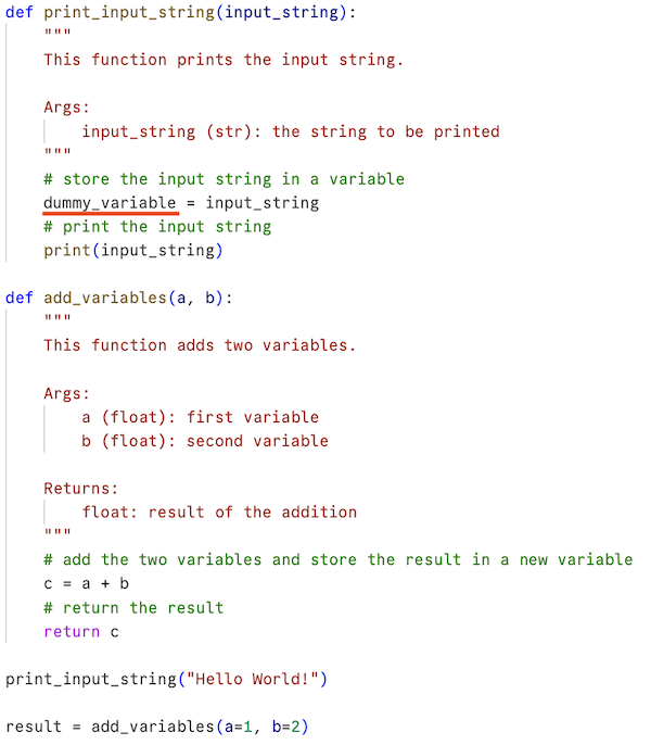
(a) An example Python script

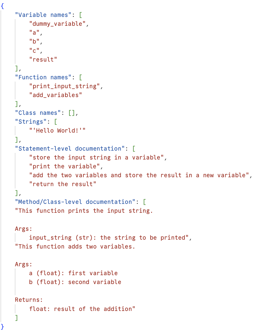
(b) Extracted identifiers

Figure 1. An example of a Python script and its extracted identifiers. The dummy_variable is underlined in red.

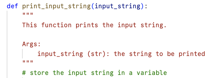
(a) Prefix

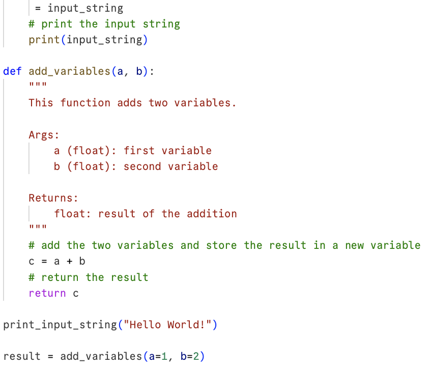
(b) Suffix

Figure 2. Prefix and suffix generated for variable dummy_variable

By breaking each script into multiple (prefix, suffix) pairs, we aim to leverage the memorization capability of LLMs. More specifically, as reported by Carlini et al. (Carlini et al., 2022), as the capacity (i.e., number of parameters) of a language model increases, so does its ability to memorize its training dataset instead of generalizing. Therefore, by using a large part of the script that was present in the model’s training dataset as input, and only masking a small piece (i.e., a single element) to be used with the FIM technique as defined in Section 3.1, the model would likely be pushed in the direction of generating an output that is the same or highly similar to the original masked token if the script was included in its training dataset (Tirumala et al., 2022).

Once we have collected all the model’s outputs for the extracted elements of a script, we look for the degree of similarity between the generated outputs and the original masked elements to determine dataset inclusion which we will explain in detail in Section 3.3.3. After obtaining the results of similarity comparison, a classification model predicts whether a project was included in a model’s training dataset given the results of similarity comparison as input.

3.3. Methodology

In this section, we will explain how TraWiC can be used for the task of dataset inclusion detection in detail. TraWiC’s pipeline consists of four stages: pre-processing, inference, comparison, and classification. Figure 3 provides an overview of our approach.

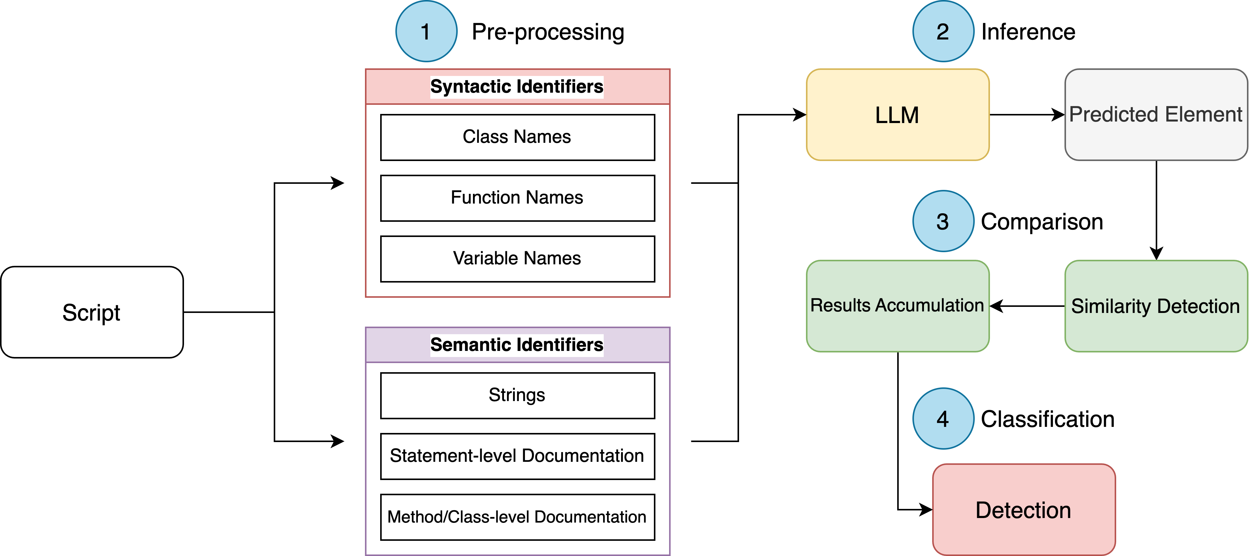
Figure 3. TraWiC’s dataset inclusion detection pipeline

3.3.1. Pre-processing

As stated in Section 3.1, we break each script into its six constituent elements (i.e., syntactic/semantic identifiers). From each script, we extract the elements and for each extracted element, we break down the script into two parts: prefix and suffix. By creating a prefix and suffix pair for each extracted element, we will be able to query the model to predict what comes in between the prefix and suffix. Algorithm 1 describes this pre-processing step in detail.

Input: SCRIPT ;

  /* SCRIPT is an entire script from a project. A project can contain many scripts. */

Output: ProcessedScript ;

  /* A list containing all the (prefix, suffix) tuples generated for each element from the input script. */

// Extract all syntactic and semantic identifiers from SCRIPT

identifiers $\leftarrow$ ExtractIdentifiers(SCRIPT);

// Generate prefix and suffix tuple for each identifier

foreach $i\in identifiers$ do

       $(p_{i},s_{i})\leftarrow\textnormal{{GeneratePrefixAndSuffix}}(i)$;

       store $(p_{i},s_{i},i)$ in ProcessedScript;

      

end foreach

return ProcessedScript;

Algorithm 1 Pre-processing

3.3.2. Inference

After breaking the script into (prefix, suffix, masked element) tuples as shown in Algorithm 1, the given model is queried to predict the masked element given prefix and suffix as input. From this tuple, the prefix and suffix are used for inference on the model while the masked element will be used in the next step for comparing the model’s outputs to the original masked element. This process is repeated for all of the tuples extracted from a script. Algorithm 2 describes this process. Once we have collected all the model’s predictions for each masked element, we move to the next step in which we compare the model’s predictions with the original elements.

Input: ProcessedScript ;

  /* Output of Algorithm 1. */

Output: ModelPredictions ;

  /* A list containing all of the given model’s predictions for the masked element. */

// Predict the masked element given prefix and suffix for the corresponding element as input

foreach $(p_{i},s_{i},i)\in ProcessedScript$ do

       $o_{i}\leftarrow\textnormal{{Predict}}(p_{i},s_{i})$;

       store $(o_{i},i,type_{i})$ in ModelPredictions;

      

end foreach

return ModelPredictions;

Algorithm 2 Inference

3.3.3. Comparison

Given the outputs of the model for each element, we define two different comparison criteria given an element’s type:

• For syntactic identifiers (Variable/Function/Class names), we look for an exact match. If the model generates the exact same token(s), we count it as a “hit”, which is a binary flag that indicates whether the generated output matches the desired output.

• For semantic identifiers (strings/documentation), to assess the similarity between two sequences (series of tokens), we use the Levenshtein distance (edit distance) score (Levenshtein, 1966). This metric measures the number of single-character edits that are required to change one sequence to the other. These elements are closer to natural language and do not require the syntactic restrictions required for code (incorrect/inaccurate generations will not result in syntax errors). Therefore, we compare the generated output with the original elements and calculate the edit distance between the two. Here, we define a threshold, and edit distances higher than this threshold will be considered as a hit. The final threshold was chosen empirically to provide a balance between semantic similarity and performance gains. We present the results with different thresholds in Section 5.

  The other metrics that can be used for this objective are based on semantic similarity where a semantic score is calculated between the vector representations of two strings (e.g., cosine similarity, TF-IDF distance, etc.) (Wang and Dong, 2020). We choose the edit distance metric as we do not aim to inspect whether the model’s output is similar to the original masked element in meaning but in syntactic structure. Therefore, analyzing the semantic distance would not be helpful for this task.

After processing the model’s outputs as described above, we normalize the hit numbers by dividing the number of hits against the total number of checks for each type of identifier. Algorithm 3 shows the comparison process in detail. Table 1 shows a sample of the dataset that is constructed for dataset inclusion detection as an output of the comparison process for the example presented in Section 3.2.

Input: ModelPredictions ;

  /* Output of Algorithm 2. */

Output: (Hits)

// Function to update hits based on the result

Function UpdateHits($Hits,key,result$)

       $Hits[key]\leftarrow Hits[key]+result$;

      

// Initialize Hits as a dictionary for each identifier type

$Hits\leftarrow\{VariableHits:0,FunctionHits:0,ClassHits:0,StringHits:0,CommentHits:0,DocStringHits:0\}$;

// Compare the given model’s outputs $(o_{i})$ to the masked element $(i)$ depending on its $type$ (i.e., variable/function/class name or string/comment/doscstring)

foreach $(o_{i},i,type_{i})\in ModelPredictions$ do

       if $type_{i}$ is variable/function/class name then

             if $o_{i}=i$  then

                  $result\leftarrow 1$;

            else

                  $result\leftarrow 0$;

             end if

            

       end if

      if $type_{i}$ is string/comment/docstring then

             if ($SemanticComparison(o_{i},i)\geq SemanticThreshold$ then

                  $result\leftarrow 1$;

            else

                  $result\leftarrow 0$;

             end if

            

       end if

      UpdateHits($Hits,type_{i},result$);

      

end foreach

return Hits;

Algorithm 3 Comparison

Table 1. Data representation sample for the example presented in Section 3.2

Script Name Class Hits Function Hits Variable Hits String Hits Comment Hits Docstring Hits sample_project/sample.py 0 1.0 0.08 0.4 0.66 0.0

3.3.4. Classification

With our extracted features, the classifier’s task is to detect whether a script was included in the LLM’s training dataset; which makes this a binary classification problem. Any classification method, such as decision trees or Deep Neural Networks (DNN), can be used based on the desired performance. We experiment with different classification methods as explained in Section 4.3

Input: Hits ;

  /* Output of Algorithm 3. */

Output: ClassificationResults ;

  /* A binary variable with 1 indicating inclusion in the dataset and 0 otherwise. */

// Predict dataset inclusion

$ClassificationResults\leftarrow\textnormal{{ClassificationModel}}(hitType,hitCount)$;

return ClassificationResults;

Algorithm 4 Classification

4. Experimental Design

In this section, we explain our experimental design including the construction of the dataset used as the ground truth for validating our approach, the LLM under study, the classifier used for detecting dataset inclusion, and details of TraWiC’s performance comparison with a state of the art CCD approach. Specifically, we aim to answer the following Research Questions (RQs):

• RQ1 [Effectiveness]

  • RQ1a: What is TraWiC’s performance for the dataset inclusion detection task?

  • RQ1b: How does TraWiC compare against traditional CCD approaches for dataset inclusion detection?

  • RQ1c: What is the effect of using different classification methods on TraWiC’s performance?

• RQ2 [Sensitivity Analysis]

  • RQ2a: How robust is TraWiC against data obfuscation techniques?

  • RQ2b: What is the importance of each feature in detecting dataset inclusion?

• RQ3 [Error Analysis] How does the model under study make mistakes in predicting the masked element?

4.1. Dataset Construction

In order to assess our approach’s correctness, we need to have access to the dataset that an LLM was trained on. By knowing which scripts/projects were used for training the model, we can construct a ground truth for training and validating the classifier for dataset inclusion detection. To do so, we select TheStack. TheStack is a large dataset (3 terabytes) of code collected from GitHub by HuggingFace. This dataset contains codes for 30 different programming languages and 137.36 million repositories (Kocetkov et al., 2022). We focus on the Python repositories in this dataset as the data cleaning process used for the model under study which we outline in Section 4.2 is accurately replicable for Python. Given the large number of Python scripts and the data cleaning approach used for producing the training data for the LLM, some scripts within a project might be included in the LLM’s dataset while others might be excluded. Therefore, we first filter the Python projects by considering a minimum of 10 and a maximum of 50 scripts per project. We focus on projects of such scale for the following reasons:

• Our aim is to increase the likelihood that some scripts within a project might be included in the training dataset of the LLM while some from the same project might not. This will allow us to have a more diverse dataset for both script-level and project-level dataset inclusion detection as explained in Section 4.4.

• As our primary objective is to detect a project’s inclusion in the training dataset of an LLM, by not including overly large projects that contain many scripts, we will have a larger number of projects in our dataset (e.g., instead of having a project with 200 scripts, we can have 5 projects with 40 scripts).

• As we outline in Section 4.2, we have chosen a data cleaning criterion based on documentation to code ratio. Therefore, to construct a balanced dataset where projects are not documented enough or too documented, we do not include overly small projects in our dataset. As reported by Mamun et al. (Mamun et al., 2017), there exists a correlation between the size of a software project and the amount of documentation written for it. Therefore, by not including overly small projects, we will increase the likelihood of having high-quality, well-documented scripts in our dataset.

We then randomly sample from the remaining projects for constructing the dataset for inclusion detection for TraWiC and NiCad (as explained in Sections 3.3 and 4.5).

4.2. Model Under Study

For evaluating our approach, without loss of generality, we use SantaCoder (Allal et al., 2023). SantaCoder is an LLM trained by HuggingFace on TheStack for program synthesis and supports Python, Java, and JavaScript programming languages. This model was chosen as the LLM under study for the following reasons:

• TheStack is publicly available. Therefore, we can inspect the data and confirm the presence of a script in SantaCoder’s training dataset.

• SantaCoder’s data cleaning procedure is clearly explained and replicable with different cleaning criteria being applied (Allal et al., 2023). To clean the data for SantaCoder’s training dataset, its developers have used: 1) “GitHub stars” which filters repositories based on the number of their stars, 2) “Comment-to-code-ratio” which considers the script’s inclusion based on the ratio of comment characters to code characters, and 3) “more near-deduplication” which employs multiple different deduplication settings. Hence, given that we have access to the original dataset, we can reproduce the dataset that the model was trained on by following the same procedures.

HuggingFace has released multiple versions of SantaCoder. Each model is trained on data that were constructed using different data-cleaning criteria. For our experiments, we chose the comment_to_code model because the comment-to-code ratio for this model is calculated by “using the ast and tokenize modules to extract docstrings and comments from Python files” (Allal et al., 2023); which allows us to accurately reproduce the data. Following the data cleaning steps outlined in (Allal et al., 2023), the training dataset for this version was constructed by filtering any script in TheStack that has a comment-to-code ratio between 1% and 80% on a character level after the standard data cleaning steps (removing files from opt-out requests, near-deduplication, PII-reduction, etc).

4.3. Classifier for Dataset Inclusion Detection

We have chosen to use random forests as the classifier for our experiments for the following reasons:

• We emphasize the need for our approach to maintain a high degree of interpretability. By using multiple decision trees (which are inherently interpretable) that comprise the random forest, this type of classifier provides interpretability alongside high classification performance.

• Ensemble methods such as random forests are known for their superior performance over single predictors due to their ability to reduce overfitting and improve generalization. They are also more computationally efficient compared to the intensive resource demands of training and inference of DNN models (LeCun et al., 2015).

To ensure a thorough comparative analysis of classifiers, we have also experimented with XGBoost (XGB) and Support Vector Machine (SVM) classifiers. For optimal classifier selection, we employed the grid search methodology which involves an exhaustive exploration of hyperparameters (LeCun et al., 2015), where for each model, we evaluated various combinations of settings. We lay out the different sets of configurations used for grid search for each model in Appendix (Section 10). The best models were selected based on the achieved F-score on the test dataset.

4.4. Detecting Dataset Inclusion

Depending on the data cleaning criteria used for filtering the scripts for training the LLM as mentioned in Section 4.2, some scripts in a project may not be included in the model’s training dataset, e.g., out of 20 scripts in a project, some may not pass the data filtering criteria. Therefore, we outline two different levels of granularity for predicting whether a project was present in a model’s training dataset:

• File-level granularity: We determine whether a single script has been in the LLM’s training dataset.

• Repository-level granularity: We analyze all the scripts from a repository and consider that the repository has been included in the LLM’s training dataset if the classifier predicts a certain amount of scripts out of the total number of scripts in the repository as being in the training dataset.

To analyze the impact of edit distance on the classifier’s performance, we define multiple levels of edit distance for a thorough sensitivity analysis. Our analysis was carried out across 263 repositories extracted from TheStack which brings us to a total of 9,409 scripts.

4.5. Comparison With Clone Detection Approaches

In software auditing, one of the approaches for detecting copyright infringement is using CCDs to check the code against a repository of copyrighted code (Ralhan and Malik, 2021). CCD is an active area of research and different approaches are proposed for the detection of clones, especially those of Type 3 and Type 4 (Ain et al., 2019). This process is carried out through a pair-wise comparison of the codes in a project against another dataset that contains copyrighted codes. As detailed in Section 2.2, many different approaches are proposed and available for CCD (Ain et al., 2019). Out of the proposed approaches, we choose NiCad (Roy and Cordy, 2008) for comparison with TraWiC on the dataset inclusion task, for the following reasons:

• Python support: Out of the proposed, available approaches, NiCad is the only one that supports clone detection for Python scripts.

• Availability: A few of the proposed approaches are available for use. Furthermore, most of them require expensive re-training on new datasets. However, NiCad is open-source and does not require re-training (as opposed to the proposed ML-based solutions).

• Syntactic errors in generated codes: Most of the proposed approaches for CCD based on DNNs, extract information such as ASTs from the code which can only be done if the generated code is syntactically valid. Even though LLMs have shown a high capability in generating correct code, limiting CCD to codes that are syntactically valid would severely reduce the size of the dataset that can be used for this study.

NiCad employs a parser-based, language-specific approach using the TXL transformation system to extract and normalize potential code clones. It is capable of detecting code clones up to Type 3 (Roy and Cordy, 2008). As NiCad is designed to detect clones between scripts, it operates differently compared to our approach where we inspect the similarity between one or multiple generated tokens. Therefore, to determine whether a code was in a model’s training dataset with NiCad, we query the model to generate code snippets and compare the generated codes against each snippet that we know exists in the model’s training dataset. We generate code snippets instead of tokens since comparing scripts to each other using NiCad will result in positive clone matches as a large portion of both scripts will be the same. Algorithm 5, shows the steps for dataset inclusion detection using NiCad. Our detailed process is as follows:

4.5.1. Pre-processing

We extract the functions and classes that are defined in a script by parsing its code. For example, the script in Figure 1a, has 2 functions. After doing so, we break each function/class into two parts based on its number of lines. Figure 4 displays an example of how this process is carried out. This process is repeated for every function and class that is extracted from the script. We consider the first half as the prefix and the second half as the suffix.

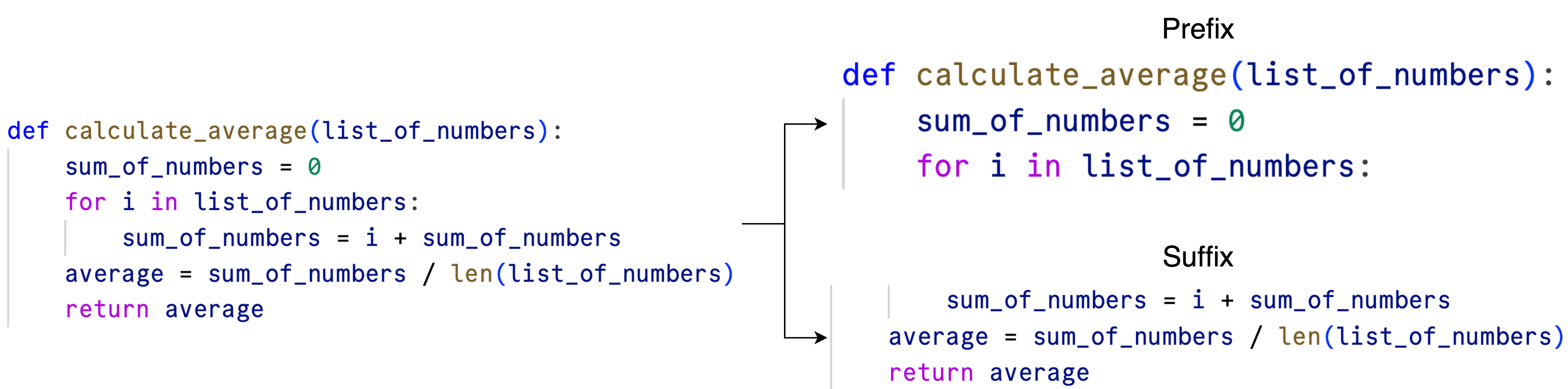
Figure 4. An example of how prefix and suffix are generated for NiCad

4.5.2. Inference

After generating prefix and suffix pairs, we query the model with the prefix and have the model generate the suffix. Note that here, we do not restrict the model to predict the masked element by giving it the suffix. Instead, we allow the model to generate what comes after the prefix until the model itself generates an “end-of-sequence” token.

4.5.3. Comparison

TheStack dataset contains 106.91 million Python scripts (Kocetkov et al., 2022). Therefore, comparing each generated script by the model under study in a pair-wise manner against all the other scripts present in the training dataset is computationally infeasible. As such, we compare each generated script with those of multiple randomly sampled repositories from the model’s training dataset to detect code clones across projects. Here, we aim to investigate whether the model generates codes from its training dataset when it is given a large part of a script as input. If NiCad detects a clone between the generated script and another script from the sampled projects, we consider it as a hit for detecting that the project was included in the model’s training dataset. As we are sampling randomly, there exists the possibility that the model generates code from its training dataset but the generated code wasn’t compared against the project that it was generated from. Therefore, to decrease the likelihood of such cases we do the following:

• We follow the same project selection criteria as described in Section 4.1 for both selecting the scripts to generate code from and comparing the generated codes against. By only sampling projects that contain a minimum of 10 and a maximum of 50 scripts, we aim to decrease the amount of missing hits.

• As we expand upon in Section 5.1.2 we experiment with multiple random sampling ratios in order to have a comprehensive sensitivity analysis.

Input: SCRIPT ;

  /* SCRIPT is an entire script from a project. A project can contain many scripts. */

Output: ClassificationResults ;

  /* A binary variable with 1 indicating inclusion in the dataset and 0 otherwise. */

// Break the script into a prefix and suffix tuple based on the number of lines.

prefix, suffix $\leftarrow$ ExtractPrefixAndSuffix(SCRIPT);

// Generate the suffix by giving the model prefix as input.

GeneratedSuffix $\leftarrow$ Predict(prefix);

// Compare the generated suffix in a pair-wise manner with every script in the dataset.

foreach $s\in\text{dataset}$ do

       r $\leftarrow$ NiCad(s, GeneratedSuffix);

       Store $r$ in ClassificationResults;

      

end foreach

return ClassificationResults;

Algorithm 5 Dataset Inclusion Detection Using NiCad

5. Results and Analysis

In this section, we present our experimental results. We begin by laying out our experiment details, continue with presenting the results of our approach compared against a baseline, and conclude this section by conducting an error, feature importance, and sensitivity analysis. Our replication package is publicly accessible online (trawic, 2024).

5.1. RQ1: [Effectiveness]

The results detailed in Table 2 showcase the performance of TraWiC’s dataset inclusion detection when applied with varying edit distance thresholds. The “Considering only a single positive” criterion showcases the results on file-level granularity. We consider multiple inclusion criteria for predicting whether a repository (i.e., project) was included in the model’s training dataset as outlined in “Considering a threshold of 0.4/0.6”. “Precision” measures the percentage of correctly predicted positive observations out of all predicted positives, reflecting the classifier’s accuracy in making positive predictions. “Accuracy” gives an overall assessment, showing the ratio of correctly predicted observations to the total predictions made. The “F-score” balances precision and sensitivity (recall), offering a comprehensive metric, especially for uneven datasets. “Sensitivity” assesses the model’s capability to correctly distinguish actual positive cases, while “Specificity” measures its performance in distinguishing true negatives. We focus on the F-score as the main performance metric since SantaCoder was trained on TheStack and as a result, most scripts in the dataset would have been included in its training dataset. After F-score, we focus on sensitivity as our goal is to detect dataset inclusion; therefore, the higher the classifier’s ability to detect true positives, the more suited to our purpose it is.

5.1.1. RQ1a: What is TraWiC’s performance for the dataset inclusion task?

We observe that the best performance in detecting dataset inclusion is achieved with an edit distance of 60 and considering a repository inclusion threshold of 0.4. We can observe that precision, accuracy, and F-score generally decrease as the edit distance threshold increases. This shows that a higher threshold for edit distance may lead to less strict matching criteria, which in turn could result in more false positives and reduce TraWiC’s performance. Additionally, we observe that sensitivity marginally increases as the edit distance threshold does. Suggesting that while the classifier may become less precise, it does not miss as many true positives at higher thresholds.

Examining Table 2, we observe diverse results based on different edit distance thresholds and repository inclusion criteria. The highest F-score, 88.57%, is achieved at an edit distance threshold of 20 when considering a single script’s inclusion. Specificity is highest, 71.6%, with the same criteria, indicating a decent balance in predicting when a script was not included in the model’s training dataset. For project inclusion detection, we report a sensitivity of 99.19% and a specificity of 2.92% while considering an edit distance threshold of 60. This means that TraWiC has a high capability in detecting whether a project was included in the training dataset. As mentioned in Section 4.4 after following the data cleaning criteria as laid out in (Allal et al., 2023) some scripts from a project may not be included in the training dataset of the given model. For example, out of the 20 scripts in a project, 10 may not have a comment-to-code ratio between 1% to 80% and therefore will not be used for training the model. Therefore, even though the project itself was included in the model’s training dataset, a specific script from it may not be. As such, it should be noted that most of the projects in our dataset (in contrast to scripts) were included in SantaCoder’s training dataset and a low specificity when it comes to project inclusion detection (as opposed to script inclusion detection) is not alarming as other scripts from the project could have been used in the model’s training.

Given the differences between TraWiC’s specificity and sensitivity on file-level granularity in comparison to repository-level granularity, we can infer two scenarios for using TraWiC. First, if a repository contains a large number of scripts and inference on the given model is resource-intensive, using TraWiC on less than half of the repository’s scripts can effectively indicate dataset inclusion. Second, in scenarios where reducing false negatives is more important (e.g., identifying every instance of dataset inclusion), applying TraWiC on file-level granularity can be an effective method to check for dataset inclusion.

Table 2. Results of TraWiC’s code inclusion detection with different edit distance thresholds

Edit Distance Threshold	Repository Inclusion Criterion	Precision(%)	Accuracy(%)	F-score(%)	Sensitivity(%)	Specificity (%)
20	Considering only a single positive	88.07	83.87	88.57	89.08	71.6
	Considering a threshold of 0.4	76.52	75.1	84.82	95.13	20.63
	Considering a threshold of 0.6	80.46	71.26	80.31	80.15	47.08
40	Considering only a single positive	79.57	79.11	83.39	94.49	42.91
	Considering a threshold of 0.4	72.96	72.4	83.8	98.43	3.62
	Considering a threshold of 0.6	75.5	73.96	84.1	94.9	18.65
60	Considering only a single positive	78.09	77.46	85.46	94.36	37.7
	Considering a threshold of 0.4	71.28	71.23	82.95	99.19	2.92
	Considering a threshold of 0.6	73.3	72.11	82.89	95.38	15.6
70	Considering only a single positive	78.47	78.08	85.85	94.77	38.81
	Considering a threshold of 0.4	73.3	72.83	84.17	98.83	2.11
	Considering a threshold of 0.6	75.46	74.11	84.39	95.71	15.34
80	Considering only a single positive	77.79	77.47	85.55	95.02	36.17
	Considering a threshold of 0.4	71.22	70.83	82.84	99	1.47
	Considering a threshold of 0.6	72.42	70.98	82.41	95.6	10.3

5.1.2. RQ1b: How does TraWiC compare against traditional CCD approaches for dataset inclusion detection?

Table 3 presents the results obtained when using NiCad for clone detection. We used NiCad to detect code clones across code snippets from the scripts in the LLM’s training dataset and code snippets generated by the LLM as outlined in Section 4.5. Given that our task is a binary classification, NiCad is unable to achieve the accuracy of a random classifier (50%) indicating that code clone detection approaches are not suitable for detecting dataset inclusion. This observation is consistent with the results reported in (Ciniselli et al., 2022). The highest accuracy, F-Score, and sensitivity are achieved by NiCad for clone detection when sampling 9% of the LLM’s dataset. As the results show, our approach outperforms NiCad by a large margin in detecting whether a project was included in the training dataset of SantaCoder regardless of the edit distance threshold. Moreover, using clone detection techniques for dataset inclusion detection is expensive. In fact, before using any clone detection technique, we need to generate code snippets using the LLM and once a sufficient amount of scripts are generated, compare them in a pair-wise manner with the original scripts that were used in the LLM’s training dataset. TraWiC is much less computationally expensive compared to generating multiple snippets of code from different repositories and using NiCad to detect similarities between them. For detecting dataset inclusion, TraWiC’s main performance constraint is inference on the LLM for generating the necessary tokens. In contrast, NiCad needs to compare an average of 3,000 scripts per project in a pair-wise manner for inclusion detection when considering a 10% sample of the filtered dataset on top of generating the necessary code from the LLM. As presented in Table 2, the best results are achieved when we focus on identifying the inclusion of single scripts with an edit distance threshold of 20. Our analysis results presented in Table 3 show that increasing the number of sampled repositories has only a marginal improvement on NiCad’s performance.

Table 3. NiCad’s performance on detecting clones across sampled repositories

Percentage of Dataset Sampled	Precision(%)	Accuracy(%)	F-Score(%)	Sensitivity(%)	Specificity (%)
Sampling 5% (1726 projects / $\approx$ 34600 scripts)	84.81	43.13	53.6	38.18	63.63
Sampling 9% (3108 projects / $\approx$ 62280 scripts)	86.74	47.64	56.47	41.86	72.5
Sampling 10% (3452 projects / $\approx$ 69200 scripts)	80.24	41.22	49.24	35.51	64.44

5.1.3. RQ1c: What is the effect of using different classification methods on TraWiC’s performance?

Table 4 shows the F-scores of different classification methods. As the results show, random forests outperform both XGB and SVM across all edit distance thresholds and repository inclusion criteria. We include a more detailed analysis of both XGB’s and SVM’s across different performance metrics in Section 10.

Table 4. Performance comparison of different classifiers on the generated dataset

Edit Distance Threshold	Repository Inclusion Criterion	F-score XGB(%)	F-score SVM(%)	F-score RF(%)
20	Considering only a single positive	86.04	85.53	88.57
	Considering a threshold of 0.4	83.53	82.30	84.82
	Considering a threshold of 0.6	80.53	77.95	80.31
40	Considering only a single positive	84.01	83.20	83.39
	Considering a threshold of 0.4	82.16	81.89	83.80
	Considering a threshold of 0.6	82.48	80.60	84.10
60	Considering only a single positive	82.49	82.43	85.46
	Considering a threshold of 0.4	82.18	82.20	82.95
	Considering a threshold of 0.6	82.02	82.37	82.89
70	Considering only a single positive	84.32	84.49	85.85
	Considering a threshold of 0.4	83.56	83.78	84.17
	Considering a threshold of 0.6	81.85	82.82	84.39
80	Considering only a single positive	82.78	82.22	85.55
	Considering a threshold of 0.4	82.39	81.91	82.84
	Considering a threshold of 0.6	81.23	81.24	82.41

5.2. RQ2 [Sensitivity Analysis]

In this RQ, we assess TraWiC’s robustness to data obfuscation. Afterward, we analyze the correlation between the extracted features in our dataset and discuss the feature importance of the trained classifiers.

5.2.1. RQ2a: How robust is TraWiC against data obfuscation techniques??

In this section, we analyze TraWiC’s robustness against models trained on obfuscated datasets. Data obfuscation can be used as a defense strategy against MIAs (Hu et al., 2022). For example, knowledge distillation (Shejwalkar and Houmansadr, 2021; Zheng et al., 2021) or differential privacy (Xu et al., 2019; Rosenblatt et al., 2020) can be used for training models that do not generate rare elements observed during their training. There also exists a myriad of code obfuscation techniques proposed for software copyright and vulnerability protection by making reverse-engineering the software more difficult. For example, Mixed Boolean Arithmetic methods (David et al., 2020) obfuscate the code by replacing arithmetic operations in a code with overly complex statements. Opaque Predicates approaches (Xu et al., 2016) obfuscate the code by setting only one direction of the code to be executed and insert dummy code in the part that never gets executed, therefore, making the code more complex without introducing any change to the code’s execution. Finally, other approaches alter identifiers, variables, and string literals or remove code indentation to change the code’s semantics (Sebastian et al., 2016). Approaches that use a combination of these methods (Kang et al., 2021) have been proposed for thorough code obfuscation to protect the code as well.

As such, in this section, we examine the robustness of our approach when confronted with models trained on obfuscated datasets. Such scenarios are also similar to detecting Type-2/Type-3 code clones. It should be noted that for our sensitivity analysis, we assume that the data for training the given model has already been obfuscated before training the model, therefore making it more robust against producing textual elements similar to the original unobfuscated codes. To simulate these scenarios, we introduce noise during the hit-count process for syntactic identifiers. This noise emulates situations where the LLM produces a syntactic identifier that deviates from the original, resulting in a miss. Moreover, we test the robustness of our approach in scenarios where noise is introduced during semantic identifiers’ hit count. Finally, we simulate scenarios where both syntactic and semantic identifiers have been changed in the training dataset by data obfuscation techniques. Therefore, we will be able to test TraWiC’s robustness in recognizing dataset inclusion despite deliberate obfuscations in the training dataset.

Tables 5, 6, and 7 show the results of our sensitivity analysis conducted by varying the levels of noise (with noise ratios of 0.1, 0.5, and 0.9) injected during the syntactic, semantic, and their combination’s hit-count process as mentioned above, respectively. Here, a “Noise Ratio” of 0.1 means that during the hit-count process, a hit is ignored with a probability of 10%. Similar to the analyses done in RQ1, we consider different edit distance thresholds (20, 60, and 80) for detecting semantic hits. It should be noted that we conduct our analysis on single scripts instead of projects. We also conduct analyses of different “Repository Inclusion Criterion” (i.e., considering a project to be included in the model’s training dataset if a certain amount of its corresponding scripts are detected as included in the model’s training dataset) similar to the analysis done in Table 2. We include these results in Section 10.

As expected, increasing the noise sensitivity threshold results in a decline in precision, accuracy, F-score, and sensitivity across all edit distance thresholds. This is aligned with the expectation that the introduction of noise impairs the classifier’s ability to correctly identify true positives. However, the random forest’s inherent robustness to overfitting and its ensemble nature appear to mitigate this effect to some extent, particularly at moderate levels of noise as also reported in (Ghosh et al., 2017). Finally, we observe that TraWiC’s performance degrades close to that of a random classifier when there exists a lot of noise in the dataset. This indicates that our approach is not robust against thorough data obfuscation techniques where nearly all semantic and syntactic identifiers are changed. We will discuss possible approaches for improving our approach in Section 8.

Table 5. Results of TraWiC’s dataset inclusion detection with noise injection in syntactic identifiers

Edit Distance Threshold	Noise Ratio	Precision(%)	Accuracy(%)	F-score(%)	Sensitivity(%)	Specificity (%)
20	0.1	88	83.09	88.13	88.27	70.3
	0.5	86.41	79.26	85.23	84.08	67.34
	0.9	87.8	69.04	75.11	65.62	77.49
60	0.1	79.45	78.51	86.18	94.17	39.85
	0.5	79.30	74.89	83.24	87.59	43.54
	0.9	81.82	59.73	66.37	55.83	69.37
80	0.1	78.92	78.03	85.94	94.32	37.82
	0.5	78.43	74.95	83.55	89.39	39.3
	0.9	79.11	65.69	74.38	70.18	54.24

Table 6. Results of TraWiC’s dataset inclusion detection with noise injection in semantic identifiers

Edit Distance Threshold	Noise Ratio	Precision(%)	Accuracy(%)	F-score(%)	Sensitivity(%)	Specificity (%)
20	0.1	87.19	82.29	87.62	88.04	68.08
	0.5	83.83	74.89	81.97	80.19	61.81
	0.9	81.7	51.86	55.22	41.7	76.94
60	0.1	79.63	78.67	86.26	94.1	40.59
	0.5	78.83	76.33	84.59	91.26	39.48
	0.9	78.79	74.31	82.89	87.44	41.88
80	0.1	79.31	78.88	86.51	95.14	38.75
	0.5	78.03	76.76	85.16	93.72	34.87
	0.9	78.13	75.21	83.86	90.51	37.45

Table 7. Results of TraWiC’s dataset inclusion detection with noise injection in both syntactic and semantic identifiers

Edit Distance Threshold	Noise Ratio	Precision(%)	Accuracy(%)	F-score(%)	Sensitivity(%)	Specificity (%)
20	0.1	87.16	82.07	87.45	87.74	68.08
	0.5	83.37	73.03	80.37	77.58	61.81
	0.9	85.25	50.96	52.18	37.59	83.95
60	0.1	79.1	77.87	85.76	93.65	38.93
	0.5	78.93	73.51	82.15	85.65	43.54
	0.9	81.97	54.1	58.53	45.52	75.28
80	0.1	78.34	77.39	85.59	94.32	35.61
	0.5	78.12	74.36	83.15	88.86	38.56
	0.9	82.1	57.45	63.24	51.42	72.32

Cross-analyzing the results of Tables 5 and 6 (noise on syntactic/semantic level only) with Table 2 which contains classifier’s performance on clean data provides the following observations:

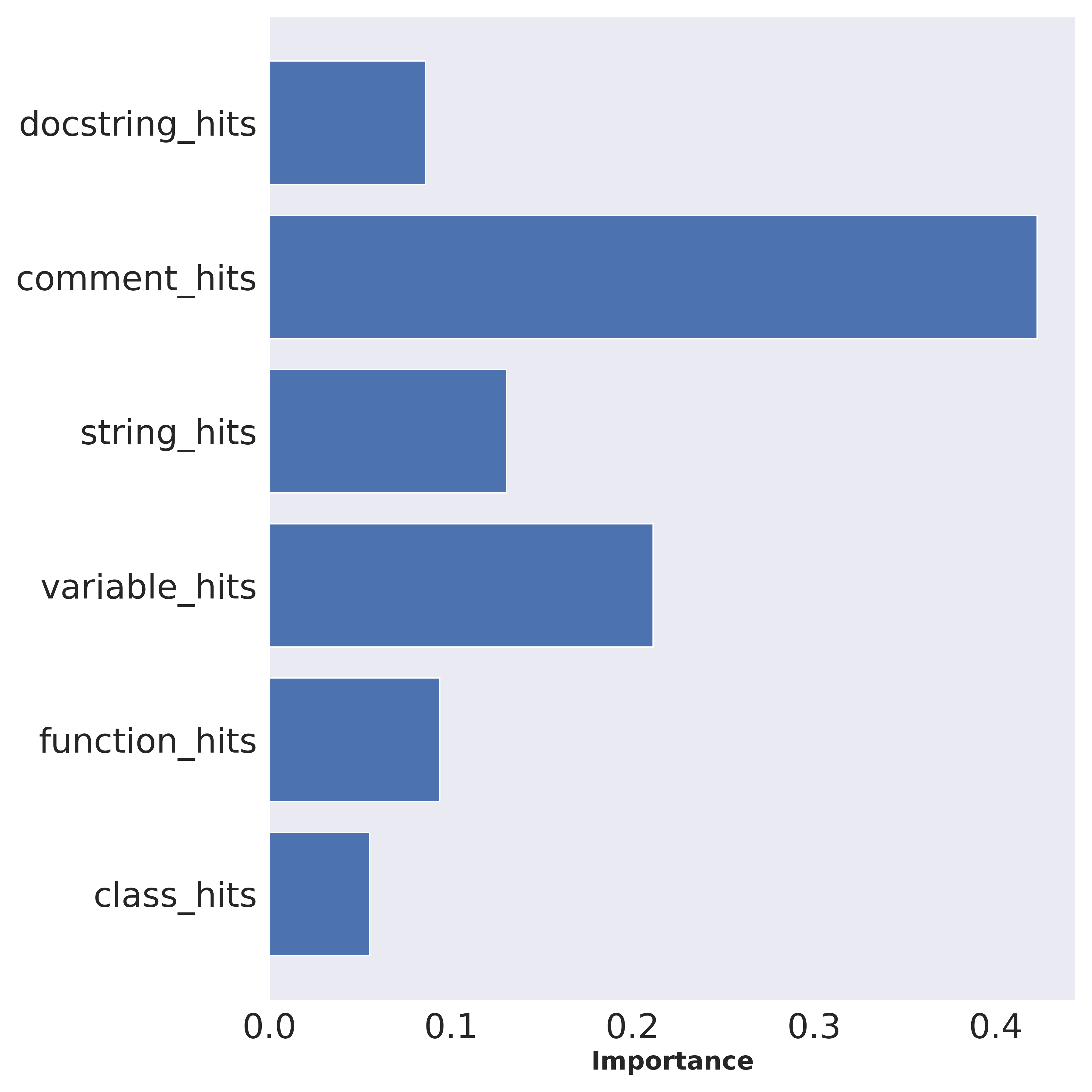
(a) Feature Importance (edit distance of 20)

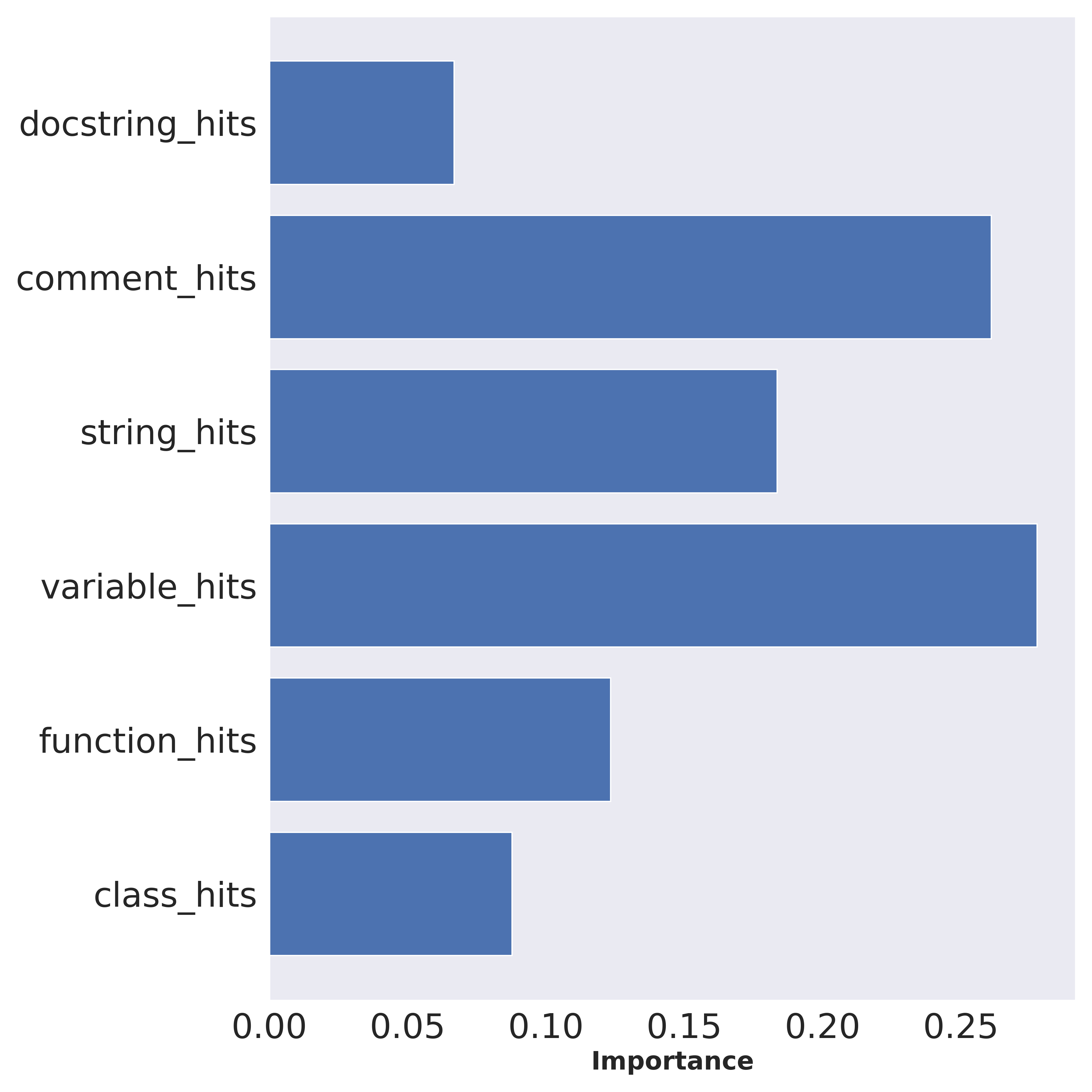
(b) Feature Importance (edit distance of 40)

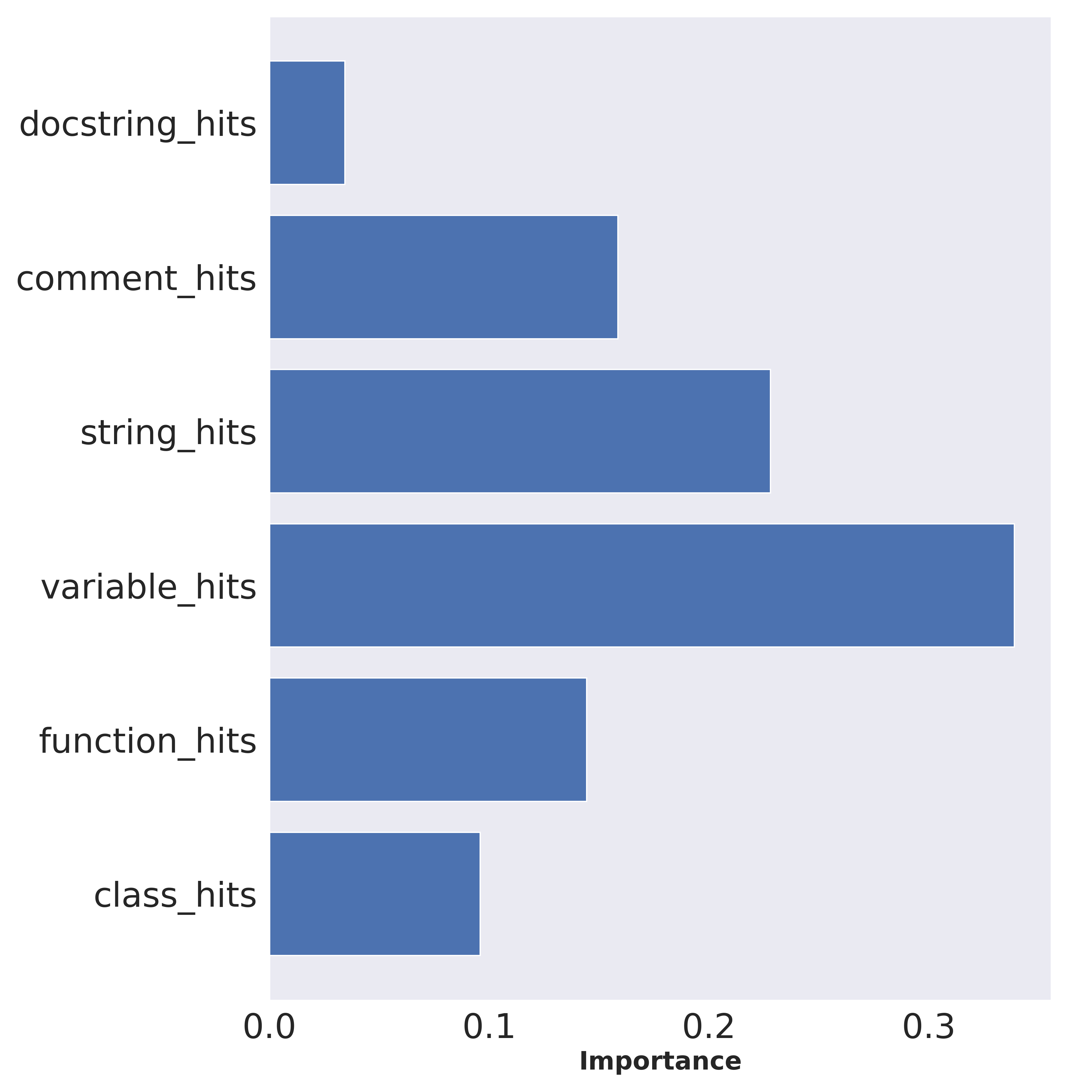
(c) Feature Importance (edit distance of 70)

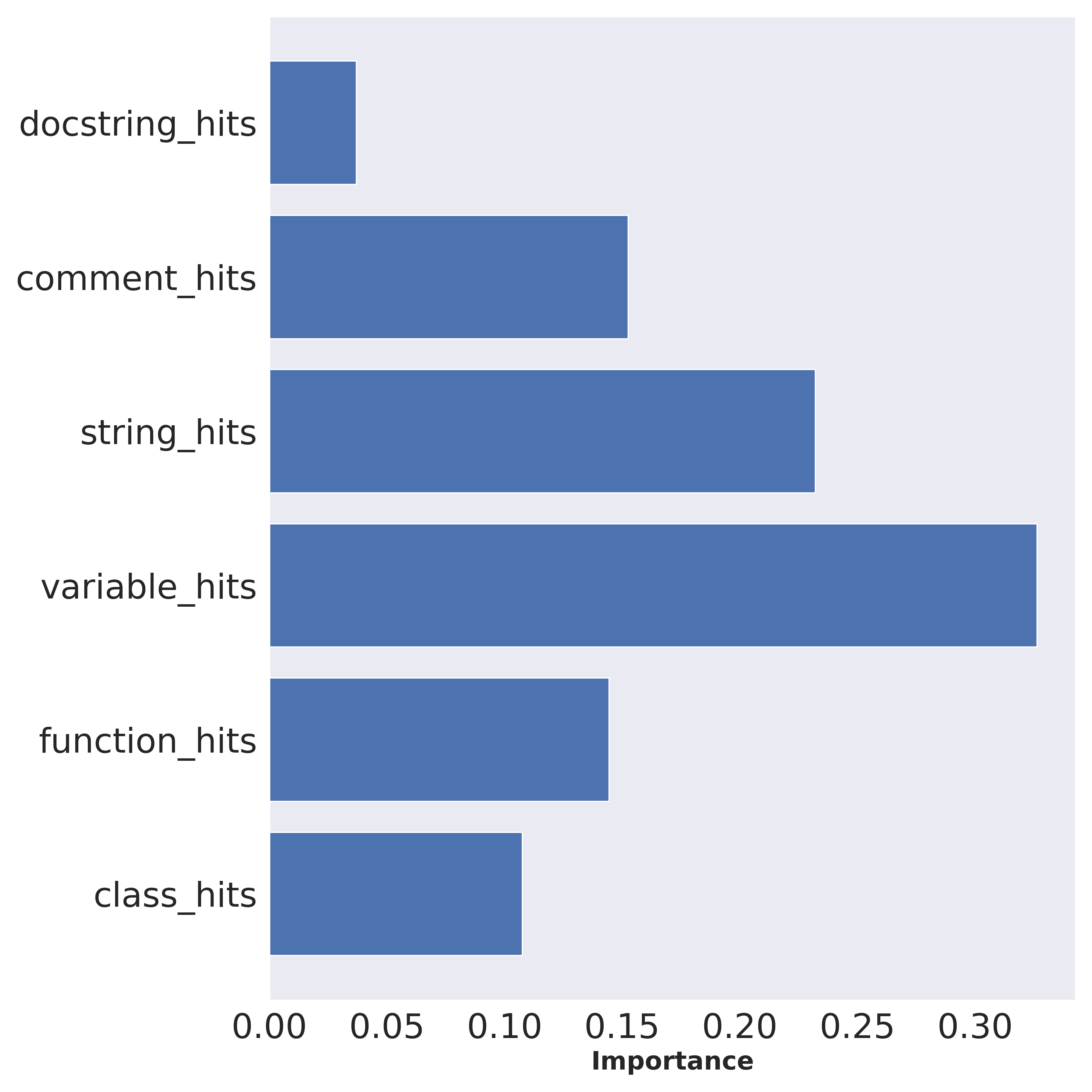
(d) Feature Importance (edit distance of 80)

Figure 5. Feature importance of the final dataset with different edit distance thresholds

• Semantic identifiers are important in dataset inclusion detection: We observe sharp degradation in the classifier’s performance at higher edit distance thresholds. As shown in Figure 5, we can observe that at lower edit distance thresholds, the classifier gives more weight to semantic identifiers compared to syntactic identifiers. Therefore, at lower edit distance thresholds, even though we observe performance degradation, the classifier has a high performance in detecting true positives even as the amount of noise is increased. As mentioned in Section 2.2, Type-2 code clones are similar to each other in syntax but have different variable/function/class names. Our results on simulating data obfuscation show that TraWiC can successfully detect dataset inclusion despite changing the syntactic identifiers.

• Considering a repository-level granularity for dataset inclusion detection can help against data obfuscation: Comparing Tables 2 and 13, one can observe degradation in detecting dataset inclusion in file-level granularity on higher edit distance thresholds. This decrease in performance is indicated by the decrease in sensitivity (correctly classified true positives) and the increase in specificity (correctly classified true negatives). As mentioned above, as a large number of the scripts in our constructed dataset have been included in the training dataset of the model under study, we cannot attribute the rise in specificity as an indicator of TraWiC’s better performance. However, even though we observe degradation in performance while considering repository-level granularity as well, we observe that analyzing all the scripts in a project can help us detect dataset inclusion even in the presence of high levels of noise. Depending on the approach used for code obfuscation, obfuscating the entire project is either too costly or adds unnecessary performance overhead to the project’s operation (Zhuang, 2018; Bunse, 2018; Sebastian et al., 2016) and many of the proposed approaches focus on obfuscating blocks of code inside the script as opposed to its entirety (Kang et al., 2021; Zhang et al., 2023). As such, even though the identifiers in one script in the project may be changed, other scripts in the same project may remain unchanged or undergo lower amounts of obfuscation, therefore, aiding in dataset inclusion detection.

5.2.2. RQ2b: What is the importance of each feature in detecting dataset inclusion?

We first analyze the constructed dataset for training the classification models using Spearman’s rank correlation coefficient (Zar, 2005) to assess the relationship between the constructed features of the dataset. Then, we analyze the classification models’ feature importance using the gini importance criterion (Breiman, 2017).

Figure 6b displays the correlation analysis of the extracted features with trained_on being the dependent variable indicating a script’s inclusion in the LLM’s training dataset. We observe weak to no correlation between different features which indicates low dependency among features and that each feature provides unique information for the classification task. As displayed in Table 2, we experiment with multiple edit distance thresholds for counting semantic hits. Even though the performances of models for different edit distance thresholds are similar, there are variations in the classifiers’ feature importance. Figure 5 displays different feature importance distributions for detecting dataset inclusion for edit distances of 20, 40, 70, and 80 respectively. As displayed in this figure, the lower the edit distance threshold is, the more the importance of docstring and comment features for deciding code inclusion increases. Comments and docstrings are specifically designed to explain the code’s functionality, as they are written to explain pieces of code in natural language, which makes them inherently unique. Therefore, with lower edit distances, which lowers the matching criterion between the original tokens and what the model generates, the number of hits for semantic elements increases, and as a result, the importance of these features increases.

Figure 6a displays the feature importance of the best-performing classifier (i.e., the random forest with an edit distance of 60 and repository inclusion criterion of 0.4). The number of variable hits is the most significant feature, followed by the number of comment hits and function hits. The number of docstring hits has the least importance, which suggests that the information within the docstrings of the code has a minimal impact on the classifier’s decisions. It should be noted that compared to other semantic identifiers, docstrings are longer (as they explain the functionality of a class alongside its inputs and outputs) and less prevalent (one per function/class). Therefore, there exists a smaller number of hits for docstrings compared to the other semantic identifiers.

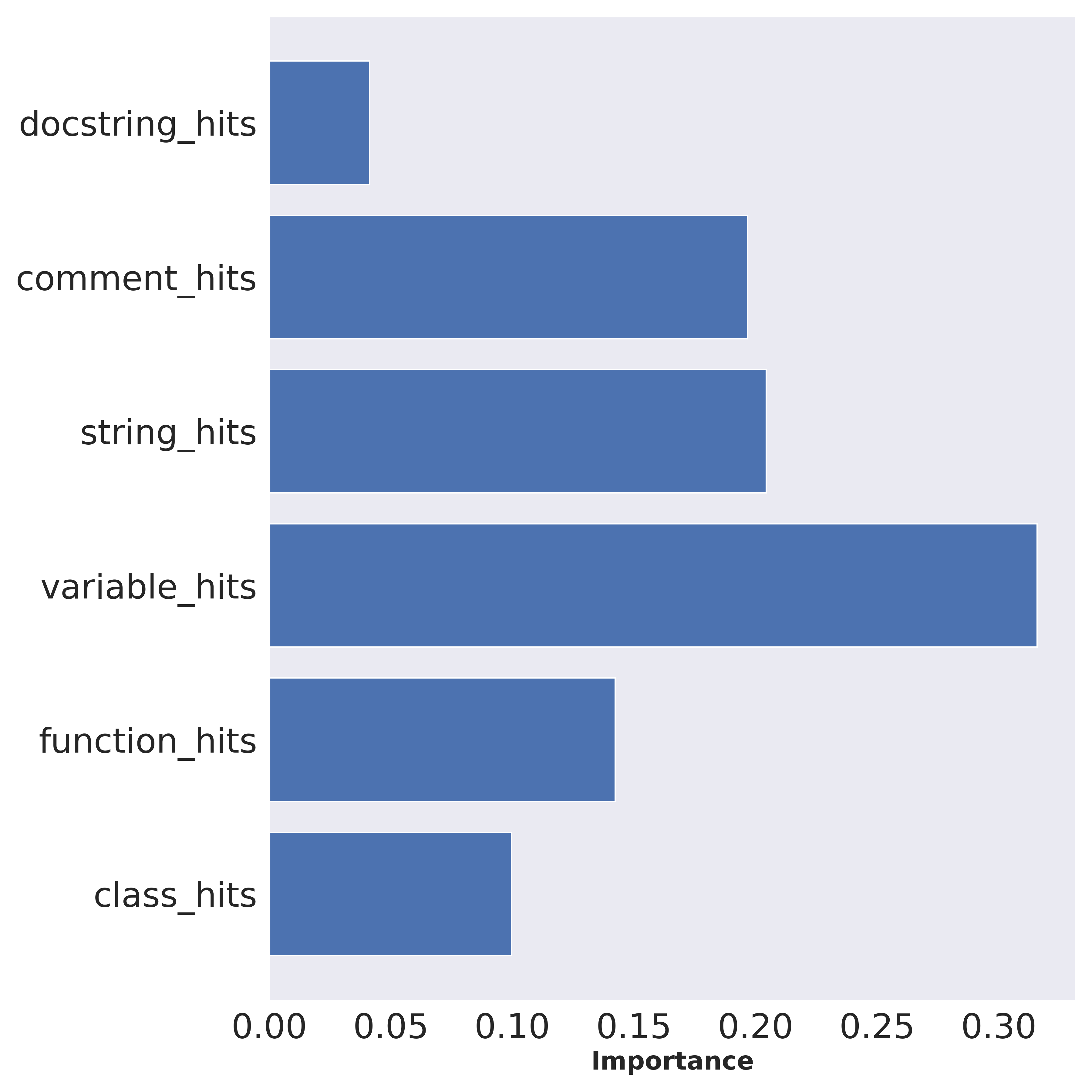
(a) Importance of each feature for detecting dataset inclusion (Considering an edit distance threshold of 60)

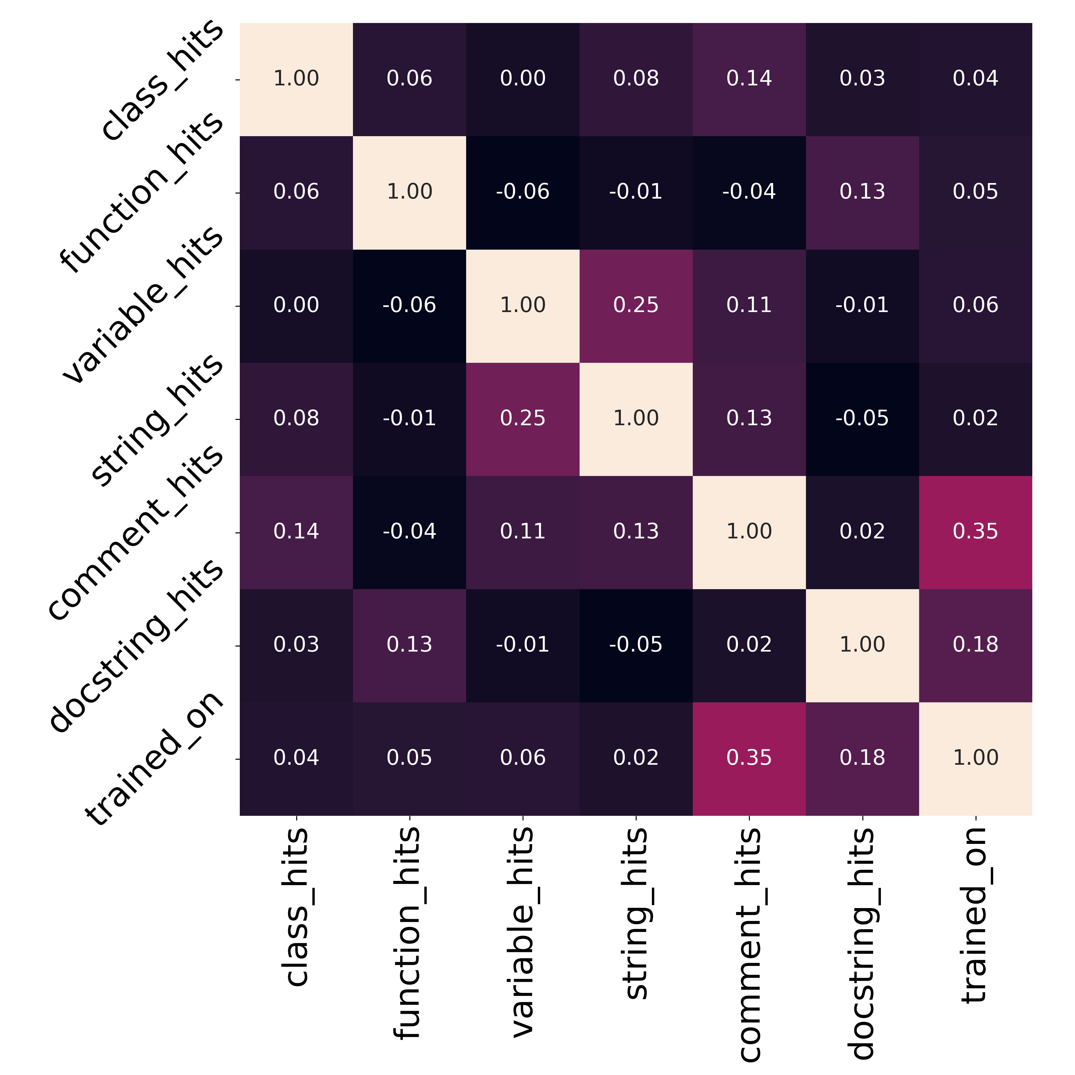
(b) Correlation of different features in the generated dataset

Figure 6. Feature importance and correlation matrix of the final dataset

5.3. RQ3: [Error Analysis]

In this RQ, we investigate how the model under study makes mistakes in predicting the masked element, and how these mistakes can be used for the task of dataset inclusion detection.

Here, we define a “mistake” as the model’s inability to generate the exact same token as what was present in the script. In Python, variable/function/class names cannot contain any white spaces between them and are considered a single token; therefore, we focus on these elements as the model’s task is predicting a single token. We observe that in most cases when the model makes a mistake, it generates the correct variable/function/class name however it also generates some extra tokens as well. Figure 7 shows an example of such cases for the variable name product_to_encode. When the model makes a mistake for syntactic identifiers, it generates an average of 23 tokens regardless of whether the underlying script was in its training dataset or not. Therefore, to understand these mistakes better, we first remove the tokens that are either a part of the programming language’s syntax or too frequent. To do so, we count the repetition frequency of each token and normalize them by dividing their repetition frequency by the total number of observed tokens. Afterward, we remove the tokens that are repeated too many times across the scripts in the dataset from the generated mistakes. The results of this analysis are presented in Table 8 with the “Filtration Threshold” column outlining the threshold for keeping a token. A filtration threshold of 0.5 means that only tokens appearing with a frequency less than or equal to 50% of all the observed tokens are retained, while tokens with a higher frequency are filtered out during the analysis.

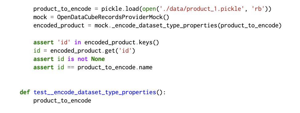
Figure 7. A case of model’s predictions for scripts not in its training data

A notable variance is observed in the class names generated by the model, with an approximate difference of around 6%, depending on whether a script was part of its training dataset or not. It is important to note that classes are less recurrent than functions and variables within code. This difference (regardless of filtration criterion) shows that MIAs, particularly when directed at rare textual elements, can serve as a means to discern the data used in a model’s training.

Table 8. Analysis of Model’s outputs by token type for scripts that are included in its training dataset

Filtration Threshold	Token Type	Output Contains Token (Script in Dataset)(%)	Output Contains Token (Script not in Dataset)(%)
0.5	Variable Names	60.71	61
	Function Names	14.08	11.77
	Class Names	11.18	5.02
0.3	Variable Names	60.89	61.38
	Function Names	15.37	12.9
	Class Names	11.3	5.08
0.1	Variable Names	60.89	60
	Function Names	15.37	11.99
	Class Names	11.3	5

6. Related Works

In this section, we review the relevant literature. Specifically, we present related works that focus on determining dataset inclusion detection for code models.

The most relevant work to our approach is the work done by Choi et al. (Choi et al., 2023) which proposes an approach for verifying whether a particular model was trained on a particular dataset. Their approach consists of investigating multiple checkpoints produced during a model’s training procedure. They show that if a model was trained on a dataset as reported by the model’s creators, then the model’s weights would “overfit” on the training dataset in the next checkpoint compared to a dataset that was not included in the training data. Even though their approach shows promising results, it requires having access to the model’s architecture, weights, hyperparameters, and training data. In comparison, TraWiC only requires query access to the given model which is the case for most of the code LLMs offered by enterprises.

Zhang et al. (Zhang and Li, 2023) proposed a framework for dataset inclusion detection on Code Pre-trained Language Models (CLPMs). In this work, the authors consider multiple levels of access to a CLPM, namely:

1. Complete access to the model and a large fraction of its training dataset (i.e., white-box access).

2. Complete access to the model’s architecture and a small fraction of its training dataset (i.e., gray-box access).

3. No access to either the model or the training dataset (i.e., black-box access).

For each level of access, they provide different detection mechanisms and their black-box level access is the setting that is comparable with TraWiC. For dataset inclusion detection given only black-box access to the model, the authors provide two methods, namely, unimodal and bimodal calibration. In unimodal calibration, the code is perturbed and the differences in the model’s output representations for different versions (e.g., uppercase vs lowercase) of the code snippet are observed. A calibration model, based on these differences, is used to infer the membership status of the code. In bimodal calibration, the calibration model’s outputs are compared to the CPLM’s outputs for the same input. This comparison is focused on identifying disparities between the two outputs, which are indicative of whether a given code snippet was used in training the CPLM or not. This method relies on the unique interaction between the natural language and programming language aspects of CPLMs, to make inferences about membership. In comparison to TraWiC, the approach proposed by Zhang et al. is focused on CLPMs that produce embeddings for downstream tasks and require expensive training of multiple large ML components (i.e., calibration models) while TraWiC is focused on LLMs that generate code. Furthermore, TraWiC is not limited to pre-trained models and does not contain any resource-intensive ML components outside of inference on the LLM itself.

Finally, Yang et al. (Yang et al., 2023) examined the risk of membership leakage in LLMs trained on code. In their approach, they assume that a fraction of the data used to train an LLM on code is available. They train a surrogate model on both said fraction and another dataset that was not included in the original model’s training. The surrogate model is supposed to mimic the behavior of the original model. Afterward, they train an MIA classifier based on the outputs of the surrogate model as an input to detect dataset inclusion. They study the results of varying degrees of membership leakage risks depending on factors such as the attacker’s knowledge of the victim model, the model’s training epochs, and the fraction of the training data that is known to the attacker. In their approach, they consider that at least a part of the training data of a model is available and it involves resource-intensive training of a surrogate model. In comparison, the main resource-intensive component of TraWiC is inference on the LLM and it does not require re-training of a surrogate model or access to the original training dataset.

7. Threats to Validity

In this section, we report on threats to the validity of our study.

Threats to internal validity concern factors internal to our study, that could have influenced our study. Our reliance on MIAs as the primary mechanism for detecting code inclusion can be considered a potential threat to the validity of our research. MIAs have been successfully used in other contexts, and our results show that leveraging MIAs is also an effective approach for detecting code inclusion. Additionally, our choice of comparison criteria for syntactic/semantic elements might not encompass all aspects of the code inclusion detection task. We mitigate this threat by experimenting with multiple values of edit distance and conducting a rigorous sensitivity analysis to show the effectiveness of our approach.

Threats to construct validity concern the relationship between theory and observation. The first threat to our construct validity involves our experimental design. To mitigate this threat and to ensure that the results of code inclusion detection were not only valid for certain scripts and projects we ran our approach using random sampling of both scripts and projects from the generated dataset to validate the results. We acknowledge that the results of detecting code inclusion using NiCad may vary as the underlying dataset is extremely large and a pair-wise comparison across the entire dataset is not feasible. We mitigate this issue by increasing the percentage of the sampled dataset to have a comprehensive analysis.

External Validity threats concern the generalization of our findings. We identify the replicability of our results as the most important external threat. Given that replicating a certain output on LLMs is difficult, we release the generated dataset, alongside TraWiC’s code (trawic, 2024). Moreover, there exists the possibility that our approach may not perform as reported on larger code models. Since SantaCoder’s introduction, many larger code models with higher performance have been introduced. It should be noted that the majority of these models are so large that they require computing resources that are not available outside of the enterprise. Furthermore, the training datasets of these large models are not available. Given such limitations, SantaCoder was the only feasible option for this study. Considering that as a model’s capacity increases so does its internal ability to remember instances from its training dataset (Carlini et al., 2022) and that our approach is model-agnostic, it is very likely that our approach would also perform well even on larger models.

8. Conclusion

In this study, we introduced TraWiC, a model-agnostic, interpretable approach for detecting code inclusion. TraWiC exploits the memorization ability of LLMs trained on code to detect whether codes from a project (collection of codes) were included in a model’s training dataset. Evaluation results show that TraWiC can detect whether a project was included in an LLM’s training dataset with a recall of up to 99.19%. Our results also show that TraWiC significantly outperforms code clone detection approaches in identifying dataset inclusion and is robust to noise. In the future, we plan to test TraWiC on more capable LLMs trained on code. We also plan to investigate what other aspects of code can be used for conducting MIAs on a code model. We aim to use deep reinforcement learning to train a model that can detect dataset inclusion based on the outputs of a code model by comparing the AST representation of the generated output to the AST representation of the input. Doing so would considerably lower TraWiC’s performance bottleneck and allow for constructing an end-to-end solution for dataset inclusion detection which is more robust against code obfuscation.

9. Acknowledgments

This work is partially supported by the Fonds de Recherche du Quebec (FRQ), the Canadian Institute for Advanced Research (CIFAR), and the Natural Sciences and Engineering Research Council of Canada (NSERC).

10. Appendix

10.1. Grid search parameters for classifiers

Here, we present the grid search parameters that were used to train the best classifiers. It should be noted that the best classifier was selected based on the highest F-score achieved on the test set. All scripts for training these models are available at (trawic, 2024).

10.1.1. Random forest

• Number of estimators: This hyperparameter is used to indicate the number of trees in the forest. We used values of 50, 100, and 200.

• Number of features for best split: The number of features to consider when looking for the best split. We used the values “sqrt” indicating the square root of the number of features in the input; and “log2” indicating the binary logarithm of the number of features in the input.

• Max tree depth: Maximum depth allowed for a single tree in the forest. we used the values of 10, 20, and 30.

• Split criterion: The function to measure the quality of a split. With “gini” indicating Gini impurity and “entropy” indicating Shannon information gain.

10.1.2. SVM

• C: The regularization parameter with the strength of regularization being inversely proportional to C. We used values of 0.1, 1, 10, 100.

• Kernel: Specifies the kernel type to be used in the algorithm. We used radial basis and linear functions.

• Kernel Coefficient: The kernel coefficient is a parameter that determines the shape of the kernel function used to map the input data into a higher-dimensional feature space. We used values of 1 , 0.1, 0.01, and 0.001.

10.1.3. XGB

• Learning rate: Also denoted as “eta” is the step size shrinkage used in the update. We used values of 0.01, 0.1, and 0.5.

• Max depth: maximum depth of a tree. We used values of 3, 5, and 7.

• Number of estimators: Number of boosting rounds or trees to build. We used values of 50, 100, and 200.

• Subsample: Subsample ratio of the training instances. For example, a subsample of 0.5 means that we randomly sample half of the training data before growing the trees. We used values of 0.6, 0.8, and 1.0.

• Subsample ratio of columns: Subsample ratio of columns when constructing each tree. Subsampling occurs once for every tree constructed. We used values of 0.6, 0.8, and 1.0.

10.2. Performance of XGB and SVM

Both SVM and XGB classifiers were trained on the same dataset as the random forest model. Tables 9 and 10 show their complete performance metrics, respectively.

Table 9. Results of TraWiC’s code inclusion detection with different edit distance thresholds - SVM

Edit Distance Threshold	Repository Inclusion Criterion	Precision(%)	Accuracy(%)	F-score(%)	Sensitivity(%)	Specificity (%)
20	Considering only a single positive	84.80	79.41	85.53	86.27	63.00
	Considering a threshold of 0.4	77.66	73.60	82.30	87.53	40.88
	Considering a threshold of 0.6	80.81	70.13	77.95	75.29	58.01
40	Considering only a single positive	74.98	73.67	83.20	93.45	27.99
	Considering a threshold of 0.4	70.66	70.30	81.89	97.37	10.11
	Considering a threshold of 0.6	72.69	69.97	80.60	90.43	24.47
60	Considering only a single positive	74.12	72.93	82.43	92.85	29.80
	Considering a threshold of 0.4	71.11	70.72	82.20	97.39	10.22
	Considering a threshold of 0.6	74.29	72.53	82.37	92.42	27.42
70	Considering only a single positive	76.60	75.00	84.49	94.19	24.95
	Considering a threshold of 0.4	73.41	72.67	83.78	97.56	7.56
	Considering a threshold of 0.6	74.87	72.19	82.82	92.67	18.60
80	Considering only a single positive	72.83	72.07	82.22	94.40	23.74
	Considering a threshold of 0.4	70.79	69.97	81.91	97.17	6.59
	Considering a threshold of 0.6	72.16	69.97	81.24	92.92	16.48

Table 10. Results of TraWiC’s code inclusion detection with different edit distance thresholds - XGB

Edit Distance Threshold	Repository Inclusion Criterion	Precision(%)	Accuracy(%)	F-score(%)	Sensitivity(%)	Specificity (%)
20	Considering only a single positive	84.94	80.05	86.04	87.18	63.00
	Considering a threshold of 0.4	77.85	75.08	83.53	90.12	39.78
	Considering a threshold of 0.6	82.31	73.27	80.53	78.82	60.22
40	Considering only a single positive	75.23	74.73	84.01	95.12	27.64
	Considering a threshold of 0.4	70.69	70.63	82.16	98.09	9.57
	Considering a threshold of 0.6	73.46	72.44	82.48	94.02	24.47
60	Considering only a single positive	73.29	72.61	82.49	94.32	25.59
	Considering a threshold of 0.4	70.58	70.39	82.18	98.34	6.99
	Considering a threshold of 0.6	72.71	71.38	82.02	94.08	19.89
70	Considering only a single positive	76.61	74.79	84.32	93.75	25.34
	Considering a threshold of 0.4	73.32	72.35	83.56	97.11	7.56
	Considering a threshold of 0.6	74.59	70.90	81.85	90.67	19.19
80	Considering only a single positive	73.38	72.98	82.78	94.95	25.42
	Considering a threshold of 0.4	71.26	70.79	82.39	97.64	8.24
	Considering a threshold of 0.6	71.87	69.80	81.23	93.40	14.84

10.3. TraWiC’s performance on different noise levels

Here, we include the complete results of TraWic’s inclusion detection against various levels of noise on script-level granularity and project-level granularity with different inclusion thresholds. Tables 11, 12, and 13 display our results on noise injected at semantic, syntactic, and both levels, respectively.

Table 11. Results of TraWiC’s code inclusion detection with different edit distance thresholds and different noise ratio - Semantic

Edit Distance Threshold	Noise Ratio	Repository Inclusion Criterion	Precision(%)	Accuracy(%)	F-score(%)	Sensitivity(%)	Specificity (%)
20	0.1	Considering only a single positive	87.19	82.29	87.62	88.04	68.08
		Considering a threshold of 0.4	79.56	76.82	86.17	93.97	20.00
		Considering a threshold of 0.6	84.55	73.51	82.30	80.17	51.43
	0.5	Considering only a single positive	83.83	74.89	81.97	80.19	61.81
		Considering a threshold of 0.4	79.14	76.82	86.27	94.83	17.14
		Considering a threshold of 0.6	85.32	74.17	82.67	80.17	54.29
	0.9	Considering only a single positive	81.70	51.86	55.22	41.70	76.94
		Considering a threshold of 0.4	80.15	75.50	85.02	90.52	25.71
		Considering a threshold of 0.6	87.18	61.59	70.10	58.62	71.43
40	0.1	Considering only a single positive	80.47	79.79	86.94	94.54	43.36
		Considering a threshold of 0.4	77.70	77.48	87.12	99.14	5.71
		Considering a threshold of 0.6	81.29	80.79	88.63	97.41	25.71
	0.5	Considering only a single positive	79.07	76.86	84.95	91.78	40.04
		Considering a threshold of 0.4	77.18	76.82	86.79	99.14	2.86
		Considering a threshold of 0.6	81.16	80.13	88.19	96.55	25.71
	0.9	Considering only a single positive	77.96	70.27	79.53	81.17	43.36
		Considering a threshold of 0.4	78.23	78.15	87.45	99.14	8.57
		Considering a threshold of 0.6	81.62	80.13	88.10	95.69	28.57
80	0.1	Considering only a single positive	79.31	78.88	86.51	95.14	38.75
		Considering a threshold of 0.4	77.70	77.48	87.12	99.14	5.71
		Considering a threshold of 0.6	80.71	80.13	88.28	97.41	22.86
	0.5	Considering only a single positive	78.03	76.76	85.16	93.72	34.87
		Considering a threshold of 0.4	77.33	77.48	87.22	100.00	2.86
		Considering a threshold of 0.6	80.71	80.13	88.28	97.41	22.86
	0.9	Considering only a single positive	78.13	75.21	83.86	90.51	37.45
		Considering a threshold of 0.4	77.85	78.15	87.55	100.00	5.71
		Considering a threshold of 0.6	81.43	81.46	89.06	98.28	25.71

Table 12. Results of TraWiC’s code inclusion detection with different edit distance thresholds and different noise ratio - Syntactic

Edit Distance Threshold	Noise Ratio	Repository Inclusion Criterion	Precision(%)	Accuracy(%)	F-score(%)	Sensitivity(%)	Specificity (%)
20	0.1	Considering only a single positive	88.00	83.09	88.13	88.27	70.30
		Considering a threshold of 0.4	79.56	76.82	86.17	93.97	20.00
		Considering a threshold of 0.6	80.73	67.55	78.22	75.86	40.00
	0.5	Considering only a single positive	86.41	79.26	85.23	84.08	67.34
		Considering a threshold of 0.4	78.68	74.83	84.92	92.24	17.14
		Considering a threshold of 0.6	81.13	66.89	77.48	74.14	42.86
	0.9	Considering only a single positive	87.80	69.04	75.11	65.62	77.49
		Considering a threshold of 0.4	78.52	74.17	84.46	91.38	17.14
		Considering a threshold of 0.6	83.51	66.23	76.06	69.83	54.29
40	0.1	Considering only a single positive	80.34	79.41	86.68	94.10	43.17
		Considering a threshold of 0.4	78.23	78.15	87.45	99.14	8.57
		Considering a threshold of 0.6	81.16	80.13	88.19	96.55	25.71
	0.5	Considering only a single positive	79.52	75.00	83.26	87.37	44.46
		Considering a threshold of 0.4	77.70	77.48	87.12	99.14	5.71
		Considering a threshold of 0.6	81.48	79.47	87.65	94.83	28.57
	0.9	Considering only a single positive	83.74	64.15	70.97	61.58	70.48
		Considering a threshold of 0.4	77.93	76.82	86.59	97.41	8.57
		Considering a threshold of 0.6	83.61	77.48	85.71	87.93	42.86
80	0.1	Considering only a single positive	78.92	78.03	85.94	94.32	37.82
		Considering a threshold of 0.4	77.85	78.15	87.55	100.00	5.71
		Considering a threshold of 0.6	80.71	80.13	88.28	97.41	22.86
	0.5	Considering only a single positive	78.43	74.95	83.55	89.39	39.30
		Considering a threshold of 0.4	77.33	77.48	87.22	100.00	2.86
		Considering a threshold of 0.6	82.01	82.12	89.41	98.28	28.57
	0.9	Considering only a single positive	79.11	65.59	74.38	70.18	54.24
		Considering a threshold of 0.4	78.38	78.81	87.88	100.00	8.57
		Considering a threshold of 0.6	82.71	80.79	88.35	94.83	34.29

Table 13. Results of TraWiC’s code inclusion detection with different edit distance thresholds and different noise ratio - Combined

Edit Distance Threshold	Noise Ratio	Repository Inclusion Criterion	Precision(%)	Accuracy(%)	F-score(%)	Sensitivity(%)	Specificity (%)
20	0.1	Considering only a single positive	87.16	82.07	87.45	87.74	68.08
		Considering a threshold of 0.4	79.71	77.48	86.61	94.83	20.00
		Considering a threshold of 0.6	83.93	73.51	82.46	81.03	48.57
	0.5	Considering only a single positive	83.37	73.03	80.37	77.58	61.81
		Considering a threshold of 0.4	79.71	77.48	86.61	94.83	20.00
		Considering a threshold of 0.6	85.45	74.83	83.19	81.03	54.29
	0.9	Considering only a single positive	85.25	50.96	52.18	37.59	83.95
		Considering a threshold of 0.4	82.11	75.50	84.52	87.07	37.14
		Considering a threshold of 0.6	87.84	60.26	68.42	56.03	74.29
40	0.1	Considering only a single positive	79.51	78.30	86.00	93.65	40.41
		Considering a threshold of 0.4	78.23	78.15	87.45	99.14	8.57
		Considering a threshold of 0.6	80.71	80.13	88.28	97.41	22.86
	0.5	Considering only a single positive	78.94	73.99	82.57	86.55	42.99
		Considering a threshold of 0.4	77.70	77.48	87.12	99.14	5.71
		Considering a threshold of 0.6	81.16	80.13	88.19	96.55	25.71
	0.9	Considering only a single positive	84.54	55.21	59.05	45.37	79.52
		Considering a threshold of 0.4	79.43	78.15	87.16	96.55	17.14
		Considering a threshold of 0.6	80.95	66.23	76.92	73.28	42.86
80	0.1	Considering only a single positive	78.34	77.39	85.59	94.32	35.61
		Considering a threshold of 0.4	77.70	77.48	87.12	99.14	5.71
		Considering a threshold of 0.6	82.01	82.12	89.41	98.28	28.57
	0.5	Considering only a single positive	78.12	74.36	83.15	88.86	38.56
		Considering a threshold of 0.4	77.70	77.48	87.12	99.14	5.71
		Considering a threshold of 0.6	81.29	80.79	88.63	97.41	25.71
	0.9	Considering only a single positive	82.10	57.45	63.24	51.42	72.32
		Considering a threshold of 0.4	79.17	78.81	87.69	98.28	14.29
		Considering a threshold of 0.6	82.20	73.51	82.91	83.62	40.00

References

- (1)
- lis (2023) 2023. Common Lisp Style Guide — Common LiSP. https://lisp-lang.org/style-guide/
- pep (2023) 2023. PEP 8 – Style guide for Python code — peps.python.org. https://peps.python.org/pep-0008/
- sim (2023) 2023. Simian Similarity Analyzer. https://simian.quandarypeak.com/
- mck (2023) 2023. The state of AI in 2023: Generative AI’s breakout year. https://www.mckinsey.com/capabilities/quantumblack/our-insights/the-state-of-ai-in-2023-generative-ais-breakout-year#
- Aghajani et al. (2020) Emad Aghajani, Csaba Nagy, Mario Linares-Vásquez, Laura Moreno, Gabriele Bavota, Michele Lanza, and David C Shepherd. 2020. Software documentation: the practitioners’ perspective. In Proceedings of the ACM/IEEE 42nd International Conference on Software Engineering. 590–601.
- Aghajani et al. (2019) Emad Aghajani, Csaba Nagy, Olga Lucero Vega-Márquez, Mario Linares-Vásquez, Laura Moreno, Gabriele Bavota, and Michele Lanza. 2019. Software documentation issues unveiled. In 2019 IEEE/ACM 41st International Conference on Software Engineering (ICSE). IEEE, 1199–1210.
- Ain et al. (2019) Qurat Ul Ain, Wasi Haider Butt, Muhammad Waseem Anwar, Farooque Azam, and Bilal Maqbool. 2019. A systematic review on code clone detection. IEEE access 7 (2019), 86121–86144.
- Allal et al. (2023) Loubna Ben Allal, Raymond Li, Denis Kocetkov, Chenghao Mou, Christopher Akiki, Carlos Munoz Ferrandis, Niklas Muennighoff, Mayank Mishra, Alex Gu, Manan Dey, et al. 2023. SantaCoder: don’t reach for the stars! arXiv preprint arXiv:2301.03988 (2023).
- Anil et al. (2023) Rohan Anil, Andrew M Dai, Orhan Firat, Melvin Johnson, Dmitry Lepikhin, Alexandre Passos, Siamak Shakeri, Emanuel Taropa, Paige Bailey, Zhifeng Chen, et al. 2023. Palm 2 technical report. arXiv preprint arXiv:2305.10403 (2023).
- Austin et al. (2021) Jacob Austin, Augustus Odena, Maxwell Nye, Maarten Bosma, Henryk Michalewski, David Dohan, Ellen Jiang, Carrie Cai, Michael Terry, Quoc Le, et al. 2021. Program synthesis with large language models. arXiv preprint arXiv:2108.07732 (2021).
- Bavarian et al. (2022) Mohammad Bavarian, Heewoo Jun, Nikolas Tezak, John Schulman, Christine McLeavey, Jerry Tworek, and Mark Chen. 2022. Efficient Training of Language Models to Fill in the Middle. arXiv:2207.14255 [cs.CL]
- Breiman (2017) Leo Breiman. 2017. Classification and regression trees. Routledge.
- Brown et al. (2020) Tom B. Brown, Benjamin Mann, Nick Ryder, Melanie Subbiah, Jared Kaplan, Prafulla Dhariwal, Arvind Neelakantan, Pranav Shyam, Girish Sastry, Amanda Askell, Sandhini Agarwal, Ariel Herbert-Voss, Gretchen Krueger, Tom Henighan, Rewon Child, Aditya Ramesh, Daniel M. Ziegler, Jeffrey Wu, Clemens Winter, Christopher Hesse, Mark Chen, Eric Sigler, Mateusz Litwin, Scott Gray, Benjamin Chess, Jack Clark, Christopher Berner, Sam McCandlish, Alec Radford, Ilya Sutskever, and Dario Amodei. 2020. Language Models are Few-Shot Learners. arXiv:2005.14165 [cs.CL]
- Bunse (2018) Christian Bunse. 2018. On the impact of code obfuscation to software energy consumption. In From Science to Society: New Trends in Environmental Informatics. Springer, 239–249.
- Carlini et al. (2022) Nicholas Carlini, Daphne Ippolito, Matthew Jagielski, Katherine Lee, Florian Tramer, and Chiyuan Zhang. 2022. Quantifying memorization across neural language models. arXiv preprint arXiv:2202.07646 (2022).
- Carlini et al. (2021) Nicholas Carlini, Florian Tramer, Eric Wallace, Matthew Jagielski, Ariel Herbert-Voss, Katherine Lee, Adam Roberts, Tom Brown, Dawn Song, Ulfar Erlingsson, et al. 2021. Extracting training data from large language models. In 30th USENIX Security Symposium (USENIX Security 21). 2633–2650.
- Chang et al. (2023) Kent K Chang, Mackenzie Cramer, Sandeep Soni, and David Bamman. 2023. Speak, memory: An archaeology of books known to chatgpt/gpt-4. arXiv preprint arXiv:2305.00118 (2023).
- Chen et al. (2021) Mark Chen, Jerry Tworek, Heewoo Jun, Qiming Yuan, Henrique Ponde de Oliveira Pinto, Jared Kaplan, Harri Edwards, Yuri Burda, Nicholas Joseph, Greg Brockman, et al. 2021. Evaluating large language models trained on code. arXiv preprint arXiv:2107.03374 (2021).
- Choi et al. (2023) Dami Choi, Yonadav Shavit, and David Duvenaud. 2023. Tools for Verifying Neural Models’ Training Data. arXiv preprint arXiv:2307.00682 (2023).
- Ciniselli et al. (2022) Matteo Ciniselli, Luca Pascarella, and Gabriele Bavota. 2022. To what extent do deep learning-based code recommenders generate predictions by cloning code from the training set?. In Proceedings of the 19th International Conference on Mining Software Repositories. 167–178.
- David et al. (2020) Robin David, Luigi Coniglio, and Mariano Ceccato. 2020. Qsynth-a program synthesis based approach for binary code deobfuscation. In BAR 2020 Workshop.
- Devlin et al. (2018) Jacob Devlin, Ming-Wei Chang, Kenton Lee, and Kristina Toutanova. 2018. Bert: Pre-training of deep bidirectional transformers for language understanding. arXiv preprint arXiv:1810.04805 (2018).
- Feitelson et al. (2020) Dror G Feitelson, Ayelet Mizrahi, Nofar Noy, Aviad Ben Shabat, Or Eliyahu, and Roy Sheffer. 2020. How developers choose names. IEEE Transactions on Software Engineering 48, 1 (2020), 37–52.
- Feldman et al. (2019) Joshua Feldman, Joe Davison, and Alexander M Rush. 2019. Commonsense knowledge mining from pretrained models. arXiv preprint arXiv:1909.00505 (2019).
- Fluri et al. (2007) Beat Fluri, Michael Wursch, and Harald C Gall. 2007. Do code and comments co-evolve? on the relation between source code and comment changes. In 14th Working Conference on Reverse Engineering (WCRE 2007). IEEE, 70–79.
- Ghosh et al. (2017) Aritra Ghosh, Naresh Manwani, and PS Sastry. 2017. On the robustness of decision tree learning under label noise. In Advances in Knowledge Discovery and Data Mining: 21st Pacific-Asia Conference, PAKDD 2017, Jeju, South Korea, May 23-26, 2017, Proceedings, Part I 21. Springer, 685–697.
- Haouari et al. (2011) Dorsaf Haouari, Houari Sahraoui, and Philippe Langlais. 2011. How good is your comment? a study of comments in java programs. In 2011 International symposium on empirical software engineering and measurement. IEEE, 137–146.
- He et al. (2021) Xinlei He, Rui Wen, Yixin Wu, Michael Backes, Yun Shen, and Yang Zhang. 2021. Node-level membership inference attacks against graph neural networks. arXiv preprint arXiv:2102.05429 (2021).
- Hu et al. (2021) Hongsheng Hu, Zoran Salcic, Gillian Dobbie, Yi Chen, and Xuyun Zhang. 2021. EAR: An enhanced adversarial regularization approach against membership inference attacks. In 2021 International Joint Conference on Neural Networks (IJCNN). IEEE, 1–8.
- Hu et al. (2022) Hongsheng Hu, Zoran Salcic, Lichao Sun, Gillian Dobbie, Philip S Yu, and Xuyun Zhang. 2022. Membership inference attacks on machine learning: A survey. ACM Computing Surveys (CSUR) 54, 11s (2022), 1–37.
- Hua et al. (2020) Wei Hua, Yulei Sui, Yao Wan, Guangzhong Liu, and Guandong Xu. 2020. Fcca: Hybrid code representation for functional clone detection using attention networks. IEEE Transactions on Reliability 70, 1 (2020), 304–318.
- Hui et al. (2021) Bo Hui, Yuchen Yang, Haolin Yuan, Philippe Burlina, Neil Zhenqiang Gong, and Yinzhi Cao. 2021. Practical blind membership inference attack via differential comparisons. arXiv preprint arXiv:2101.01341 (2021).
- Jia et al. (2019) Jinyuan Jia, Ahmed Salem, Michael Backes, Yang Zhang, and Neil Zhenqiang Gong. 2019. Memguard: Defending against black-box membership inference attacks via adversarial examples. In Proceedings of the 2019 ACM SIGSAC conference on computer and communications security. 259–274.
- Kang et al. (2021) Seoyeon Kang, Sujeong Lee, Yumin Kim, Seong-Kyun Mok, and Eun-Sun Cho. 2021. Obfus: An obfuscation tool for software copyright and vulnerability protection. In Proceedings of the Eleventh ACM Conference on Data and Application Security and Privacy. 309–311.
- Kocetkov et al. (2022) Denis Kocetkov, Raymond Li, Loubna Ben Allal, Jia Li, Chenghao Mou, Carlos Muñoz Ferrandis, Yacine Jernite, Margaret Mitchell, Sean Hughes, Thomas Wolf, Dzmitry Bahdanau, Leandro von Werra, and Harm de Vries. 2022. The Stack: 3 TB of permissively licensed source code. Preprint (2022).
- LeCun et al. (2015) Yann LeCun, Yoshua Bengio, and Geoffrey Hinton. 2015. Deep learning. nature 521, 7553 (2015), 436–444.
- Leino and Fredrikson (2020) Klas Leino and Matt Fredrikson. 2020. Stolen memories: Leveraging model memorization for calibrated White-Box membership inference. In 29th USENIX security symposium (USENIX Security 20). 1605–1622.
- Levenshtein (1966) V. I. Levenshtein. 1966. Binary Codes Capable of Correcting Deletions, Insertions and Reversals. Soviet Physics Doklady 10 (Feb. 1966), 707.
- Long et al. (2018) Yunhui Long, Vincent Bindschaedler, Lei Wang, Diyue Bu, Xiaofeng Wang, Haixu Tang, Carl A Gunter, and Kai Chen. 2018. Understanding membership inferences on well-generalized learning models. arXiv preprint arXiv:1802.04889 (2018).
- Luo et al. (2023) Ziyang Luo, Can Xu, Pu Zhao, Qingfeng Sun, Xiubo Geng, Wenxiang Hu, Chongyang Tao, Jing Ma, Qingwei Lin, and Daxin Jiang. 2023. WizardCoder: Empowering Code Large Language Models with Evol-Instruct. arXiv preprint arXiv:2306.08568 (2023).
- Lutellier et al. (2020) Thibaud Lutellier, Hung Viet Pham, Lawrence Pang, Yitong Li, Moshi Wei, and Lin Tan. 2020. Coconut: combining context-aware neural translation models using ensemble for program repair. In Proceedings of the 29th ACM SIGSOFT international symposium on software testing and analysis. 101–114.
- Mamun et al. (2017) Md Abdullah Al Mamun, Christian Berger, and Jörgen Hansson. 2017. Correlations of software code metrics: an empirical study. In Proceedings of the 27th international workshop on software measurement and 12th international conference on software process and product measurement. 255–266.
- Martin (2009) Robert C Martin. 2009. Clean code: a handbook of agile software craftsmanship. Pearson Education.
- Melis et al. (2019) Luca Melis, Congzheng Song, Emiliano De Cristofaro, and Vitaly Shmatikov. 2019. Exploiting unintended feature leakage in collaborative learning. In 2019 IEEE symposium on security and privacy (SP). IEEE, 691–706.
- Peters et al. (2018) Matthew E. Peters, Mark Neumann, Mohit Iyyer, Matt Gardner, Christopher Clark, Kenton Lee, and Luke Zettlemoyer. 2018. Deep contextualized word representations. arXiv:1802.05365 [cs.CL]
- Petroni et al. (2019) Fabio Petroni, Tim Rocktäschel, Patrick Lewis, Anton Bakhtin, Yuxiang Wu, Alexander H Miller, and Sebastian Riedel. 2019. Language models as knowledge bases? arXiv preprint arXiv:1909.01066 (2019).
- Qiu et al. (2020) Xipeng Qiu, Tianxiang Sun, Yige Xu, Yunfan Shao, Ning Dai, and Xuanjing Huang. 2020. Pre-trained models for natural language processing: A survey. Science China Technological Sciences 63, 10 (2020), 1872–1897.
- Radford et al. (2019) Alec Radford, Jeff Wu, Rewon Child, David Luan, Dario Amodei, and Ilya Sutskever. 2019. Language Models are Unsupervised Multitask Learners. (2019).
- Ralhan and Malik (2021) Chavi Ralhan and Navneet Malik. 2021. A Study of Software Clone Detection Techniques for Better Software Maintenance and Reliability. In 2021 International Conference on Computing Sciences (ICCS). IEEE, 249–253.
- Rosenblatt et al. (2020) Lucas Rosenblatt, Xiaoyan Liu, Samira Pouyanfar, Eduardo de Leon, Anuj Desai, and Joshua Allen. 2020. Differentially private synthetic data: Applied evaluations and enhancements. arXiv preprint arXiv:2011.05537 (2020).
- Roy and Cordy (2007) Chanchal Kumar Roy and James R Cordy. 2007. A survey on software clone detection research. Queen’s School of computing TR 541, 115 (2007), 64–68.
- Roy and Cordy (2008) Chanchal K Roy and James R Cordy. 2008. NICAD: Accurate detection of near-miss intentional clones using flexible pretty-printing and code normalization. In 2008 16th iEEE international conference on program comprehension. IEEE, 172–181.
- Roy et al. (2009) Chanchal K Roy, James R Cordy, and Rainer Koschke. 2009. Comparison and evaluation of code clone detection techniques and tools: A qualitative approach. Science of computer programming 74, 7 (2009), 470–495.
- Rozière et al. (2023) Baptiste Rozière, Jonas Gehring, Fabian Gloeckle, Sten Sootla, Itai Gat, Xiaoqing Ellen Tan, Yossi Adi, Jingyu Liu, Tal Remez, Jérémy Rapin, Artyom Kozhevnikov, Ivan Evtimov, Joanna Bitton, Manish Bhatt, Cristian Canton Ferrer, Aaron Grattafiori, Wenhan Xiong, Alexandre Défossez, Jade Copet, Faisal Azhar, Hugo Touvron, Louis Martin, Nicolas Usunier, Thomas Scialom, and Gabriel Synnaeve. 2023. Code Llama: Open Foundation Models for Code. arXiv:2308.12950 [cs.CL]
- Saini et al. (2018) Neha Saini, Sukhdip Singh, et al. 2018. Code clones: Detection and management. Procedia computer science 132 (2018), 718–727.
- Sajnani et al. (2016) Hitesh Sajnani, Vaibhav Saini, Jeffrey Svajlenko, Chanchal K Roy, and Cristina V Lopes. 2016. Sourcerercc: Scaling code clone detection to big-code. In Proceedings of the 38th International Conference on Software Engineering. 1157–1168.
- Salem et al. (2018) Ahmed Salem, Yang Zhang, Mathias Humbert, Pascal Berrang, Mario Fritz, and Michael Backes. 2018. Ml-leaks: Model and data independent membership inference attacks and defenses on machine learning models. arXiv preprint arXiv:1806.01246 (2018).
- Sebastian et al. (2016) Savio Antony Sebastian, Saurabh Malgaonkar, Paulami Shah, Mudit Kapoor, and Tanay Parekhji. 2016. A study & review on code obfuscation. In 2016 World Conference on Futuristic Trends in Research and Innovation for Social Welfare (Startup Conclave). IEEE, 1–6.
- Services (2023) Amazon Web Services. 2023. Code references - CodeWhisperer. https://docs.aws.amazon.com/codewhisperer/latest/userguide/code-reference.html
- Shejwalkar and Houmansadr (2021) Virat Shejwalkar and Amir Houmansadr. 2021. Membership privacy for machine learning models through knowledge transfer. In Proceedings of the AAAI conference on artificial intelligence, Vol. 35. 9549–9557.
- Shokri et al. (2017) Reza Shokri, Marco Stronati, Congzheng Song, and Vitaly Shmatikov. 2017. Membership inference attacks against machine learning models. In 2017 IEEE symposium on security and privacy (SP). IEEE, 3–18.
- Tirumala et al. (2022) Kushal Tirumala, Aram Markosyan, Luke Zettlemoyer, and Armen Aghajanyan. 2022. Memorization without overfitting: Analyzing the training dynamics of large language models. Advances in Neural Information Processing Systems 35 (2022), 38274–38290.
- trawic (2024) trawic. 2024. TraWiC. https://github.com/CommissarSilver/TraWiC.
- Vaswani et al. (2023) Ashish Vaswani, Noam Shazeer, Niki Parmar, Jakob Uszkoreit, Llion Jones, Aidan N. Gomez, Lukasz Kaiser, and Illia Polosukhin. 2023. Attention Is All You Need. arXiv:1706.03762 [cs.CL]
- Wang and Dong (2020) Jiapeng Wang and Yihong Dong. 2020. Measurement of text similarity: a survey. Information 11, 9 (2020), 421.
- Xu et al. (2019) Chugui Xu, Ju Ren, Deyu Zhang, Yaoxue Zhang, Zhan Qin, and Kui Ren. 2019. GANobfuscator: Mitigating information leakage under GAN via differential privacy. IEEE Transactions on Information Forensics and Security 14, 9 (2019), 2358–2371.
- Xu et al. (2016) Dongpeng Xu, Jiang Ming, and Dinghao Wu. 2016. Generalized dynamic opaque predicates: A new control flow obfuscation method. In Information Security: 19th International Conference, ISC 2016, Honolulu, HI, USA, September 3-6, 2016. Proceedings 19. Springer, 323–342.
- Yang et al. (2023) Zhou Yang, Zhipeng Zhao, Chenyu Wang, Jieke Shi, Dongsum Kim, Donggyun Han, and David Lo. 2023. Gotcha! This Model Uses My Code! Evaluating Membership Leakage Risks in Code Models. arXiv preprint arXiv:2310.01166 (2023).
- Ying et al. (2005) Annie TT Ying, James L Wright, and Steven Abrams. 2005. Source code that talks: an exploration of Eclipse task comments and their implication to repository mining. ACM SIGSOFT software engineering notes 30, 4 (2005), 1–5.
- Zar (2005) Jerrold H Zar. 2005. Spearman rank correlation. Encyclopedia of biostatistics 7 (2005).
- Zhang et al. (2021a) Chiyuan Zhang, Samy Bengio, Moritz Hardt, Benjamin Recht, and Oriol Vinyals. 2021a. Understanding deep learning (still) requires rethinking generalization. Commun. ACM 64, 3 (2021), 107–115.
- Zhang et al. (2021b) Chiyuan Zhang, Daphne Ippolito, Katherine Lee, Matthew Jagielski, Florian Tramèr, and Nicholas Carlini. 2021b. Counterfactual memorization in neural language models. arXiv preprint arXiv:2112.12938 (2021).
- Zhang et al. (2019) Jian Zhang, Xu Wang, Hongyu Zhang, Hailong Sun, Kaixuan Wang, and Xudong Liu. 2019. A novel neural source code representation based on abstract syntax tree. In Proceedings of the 41st International Conference on Software Engineering. IEEE Press, 783–794.
- Zhang et al. (2023) Peihua Zhang, Chenggang Wu, Mingfan Peng, Kai Zeng, Ding Yu, Yuanming Lai, Yan Kang, Wei Wang, and Zhe Wang. 2023. Khaos: The Impact of Inter-procedural Code Obfuscation on Binary Diffing Techniques. In Proceedings of the 21st ACM/IEEE International Symposium on Code Generation and Optimization. 55–67.
- Zhang and Li (2023) Sheng Zhang and Hui Li. 2023. Code Membership Inference for Detecting Unauthorized Data Use in Code Pre-trained Language Models. arXiv preprint arXiv:2312.07200 (2023).
- Zheng et al. (2021) Junxiang Zheng, Yongzhi Cao, and Hanpin Wang. 2021. Resisting membership inference attacks through knowledge distillation. Neurocomputing 452 (2021), 114–126.
- Zhuang (2018) Yan Zhuang. 2018. The performance cost of software obfuscation for Android applications. Computers & Security 73 (2018), 57–72.