Integrating ytopt and libEnsemble to Autotune OpenMC

Abstract

ytopt is a Python machine-learning-based autotuning software package developed within the ECP PROTEAS-TUNE project. The ytopt software adopts an asynchronous search framework that consists of sampling a small number of input parameter configurations and progressively fitting a surrogate model over the input-output space until exhausting the user-defined maximum number of evaluations or the wall-clock time. libEnsemble is a Python toolkit for coordinating workflows of asynchronous and dynamic ensembles of calculations across massively parallel resources developed within the ECP PETSc/TAO project. libEnsemble helps users take advantage of massively parallel resources to solve design, decision, and inference problems and expands the class of problems that can benefit from increased parallelism. In this paper we present our methodology and framework to integrate ytopt and libEnsemble to take advantage of massively parallel resources to accelerate the autotuning process. Specifically, we focus on using the proposed framework to autotune the ECP ExaSMR application OpenMC, an open source Monte Carlo particle transport code. OpenMC has seven tunable parameters some of which have large ranges such as the number of particles in-flight, which is in the range of 100,000 to 8 million, with its default setting of 1 million. Setting the proper combination of these parameter values to achieve the best performance is extremely time-consuming. Therefore, we apply the proposed framework to autotune the MPI/OpenMP offload version of OpenMC based on a user-defined metric such as the figure of merit (FoM) (particles/s) or energy efficiency energy-delay product (EDF) on the OLCF Frontier TDS system Crusher. The experimental results show that we achieve improvement up to 29.49% in FoM and up to 30.44% in EDP.

1 Introduction

As we have entered the exascale computing era, high performance, power, and energy management are still key design points and constraints for any next generation of large-scale high-performance computing (HPC) systems. Efficiently utilizing procured power and optimizing the performance of scientific applications under power and energy constraints are still challenging for several reasons, including dynamic phase behavior, manufacturing variation, and increasing system-level heterogeneity. As the complexity of such HPC ecosystems (hardware stack, software stack, applications) continues to rise, achieving optimal performance and energy becomes a challenge. The number of tunable parameters that HPC users can configure at the system and application levels has increased significantly, resulting in a dramatically increased parameter space. Exhaustively evaluating all parameter combinations becomes very time-consuming. Therefore, autotuning for automatic exploration of the parameter space is necessary.

Autotuning is an approach that explores a search space of tunable parameter configurations of an application efficiently executed on an HPC system. Typically, one selects and evaluates a subset of the configurations on the target system and/or uses analytical models to identify the best implementation or configuration for performance or energy within a given computational budget. Such methods are becoming too difficult in practice, however, because of the hardware, software, and application complexity. Recently, the use of advanced search methods that adopt mathematical optimization methods to explore the search space in an intelligent way has received significant attention in the autotuning community. Such a strategy, however, requires search methods to efficiently navigate the large parameter search space of possible configurations in order to avoid a large number of time-consuming application executions to determine high-performance configurations.

In the 2022 Exascale Computing Project (ECP) [ECP(2023)]) annual meeting panel “Exascale Computing: Hits and Misses,” Prof. Jack Dongarra from the University of Tennessee, Knoxville, mentioned that, as predicted, autotuning should be ready for exascale systems, but considerable work is still needed. Traditional autotuning methods are built on heuristics that derive from automatically tuned BLAS libraries [Whaley and Dongarra(1998)], experience [Tapus(2002), Chung and Hollingsworth(2006), Gerndt and Ott(2010)], and model-based methods [Chen(2005), Tiwari and Hollingsworth(2011), Balaprakash(2013), Falch and Elster(2017)]. At the compiler level [Ashouri(2019)], methods based on machine-learning (ML) are used for automatic tuning of the iterative compilation process [Ogilvie(2017)] and tuning of compiler-generated code [Tiwari(2009), Muralidharan(2014)]. Autotuning OpenMP codes went beyond loop schedules to look at parallel tasks and function inlining [Sreenivasan(2019), Katarzynski and Cytowski(2014), Mustafa(2011), Liao(2010)]. Recent work on leveraging Bayesian optimization to explore the parameter space search showed the potential for autotuning on CPU systems [Wu(2020), Wu(2022), Liu(2021), Roy(2021)] and on GPU systems [Miyazaki(2018), Willemsen(2021)]. Most of the autotuning frameworks mentioned above were for autotuning on a single node or a few compute nodes using only the application runtime as the performance metric. Recently, new autotuning frameworks are emerging for multinode autotuning. For example, GPtune [Liu(2021)] autotuned some MPI applications on up to 64 nodes with 2,048 cores with multitask learning using MPI, and Bayesian optimization was applied to increase the energy efficiency of a GPU cluster system [Miyazaki(2018)].

Our recent effort, yopt [Wu(2023), Wu(2022), ytopt(2023)], which is one of the ECP PROTEAS-TUNE projects [PROTEAS-TUNE(2023)], is an ML-based autotuning software package that consists of sampling a small number of input parameter configurations, evaluating them, and progressively fitting a surrogate model over the input-output space until exhausting the user-defined maximum number of evaluations or the wall-clock time. ytopt had already been applied to autotune PolyBench benchmarks with LLVM Clang/Polly loop optimization pragmas and hyperparameter optimization for deep learning applications [Wu(2022)] and Apache TVM-based scientific applications [Wu(2023a)]. In our previous work [Wu(2023)] we used ytopt to autotune four hybrid MPI/OpenMP ECP proxy applications [ProxyApps(2022)] at large scales. We used Bayesian optimization with a random forest surrogate model to effectively search the parameter spaces with up to 6 million different configurations. By using ytopt to identify the best configuration, we achieved up to 91.59% performance improvement, up to 21.2% energy savings, and up to 37.84% EDP improvement on up to 4,096 nodes.

Nevertheless, our current ytopt has several limitations. It evaluates one parameter configuration each time. This affects the effectiveness of identifying the promising search regions at the beginning of the autotuning process because of few data points being available for training the random forest surrogate model. This one-by-one evaluation process is time-consuming. There is a need for ytopt to parallelize the multiple independent evaluations in order to accelerate the autotuning process. Some of the initial random selected configurations may result in much larger execution time than the baseline one as we had in [Wu(2023)]; there is also a need for ytopt to set a proper evaluation timeout in order to evaluate more good configurations. These are the main motivations for the work reported here.

libEnsemble [Hudson(2021), Hudson(2023)], which is part of the ECP PETSc/TAO project [PETSC/TAO(2023)], is a Python toolkit for coordinating workflows of asynchronous and dynamic ensembles of calculations across massively parallel resources. libEnsemble helps users take advantage of massively parallel resources to solve design, decision, and inference problems and expands the class of problems that can benefit from increased parallelism. libEnsemble employs a manager/worker scheme that communicates via MPI, multiprocessing, or TCP.

To cope with the limitations of ytopt mentioned earlier, based on our previous work on autotuning the performance, power, and energy of applications and systems [Wu(2023), Wu(2022), Wu(2020)], we propose an asynchronously autotuning framework ytopt-libe by integrating ytopt and libEnsemble. The framework ytopt-libe comprises two asynchronous aspects:

• The asynchronous aspect of the search allows the search to avoid waiting for all the evaluation results before proceeding to the next iteration. As soon as an evaluation is finished, the data is used to retrain the surrogate model, which is then used to bias the search toward the promising configurations.

• The asynchronous aspect of the evaluation allows ytopt to evaluate multiple selected parameter configurations in parallel by using the asynchronous and dynamic manager/worker scheme in libEnsemble. All workers are independent; there is no direct communication among them. When a worker finishes an evaluation, it sends its result back to ytopt. Then ytopt updates the surrogate model and selects a new configuration for the worker to evaluate.

The advantages of this proposed autotuning framework ytopt-libe are threefold:

• Exploit the asynchronous and dynamic task management features provided by libEnsemble

• Accelerate the evaluation process of ytopt to take advantage of massively parallel resources by overlapping multiple evaluations in parallel

• Improve the accuracy of the random forest surrogate model by feeding more data to make the ytopt search more efficient.

OpenMC [Romano(2015), Tramm(2022)] is a community developed Monte Carlo neutral transport code. Recent years have seen development and optimization of this code for GPUs via the OpenMP target offloading model, as part of the ECP ExaSMR project [ExaSMR(2023)]. In this paper we apply the proposed framework ytopt-libe to autotune OpenMC to evaluate its effectiveness on an ECP system Crusher [Crusher(2023)], which is a Frontier test and development system at the Oak Ridge Leadership Computing Facility (OLCF).

The remainder of this paper is organized as follows. Section 2 discusses the background, challenges, and motivation of this study. Section 3 proposes our autotuning framework for integrating ytopt and libEnsemble. Section 4 describes the OLCF Frontier TDS system Crusher and its power measurement. Section 5 describes the ECP application OpenMC and defines its parameter space. Section 6 illustrates autotuning in performance based on the figure of merit (FoM) of OpenMC. Section 7 presents autotuning in the runtime, energy, and energy delay product (EDP). Section 8 summarizes this paper.

2 Backgrounds

In this section we briefly discuss some background about ytopt and libEnsemble.

2.1 ytopt: ML-Based Autotuning Software

yopt [Wu(2023), Wu(2022), ytopt(2023)], which is one of ECP PROTEAS-TUNE project [PROTEAS-TUNE(2023)], is a ML-based autotuning software package that consists of sampling a small number of input parameter configurations, evaluating them, and progressively fitting a surrogate model over the input-output space until exhausting the user-defined maximum number of evaluations or the wall-clock time. The package is built based on Bayesian optimization that solves optimization problems.

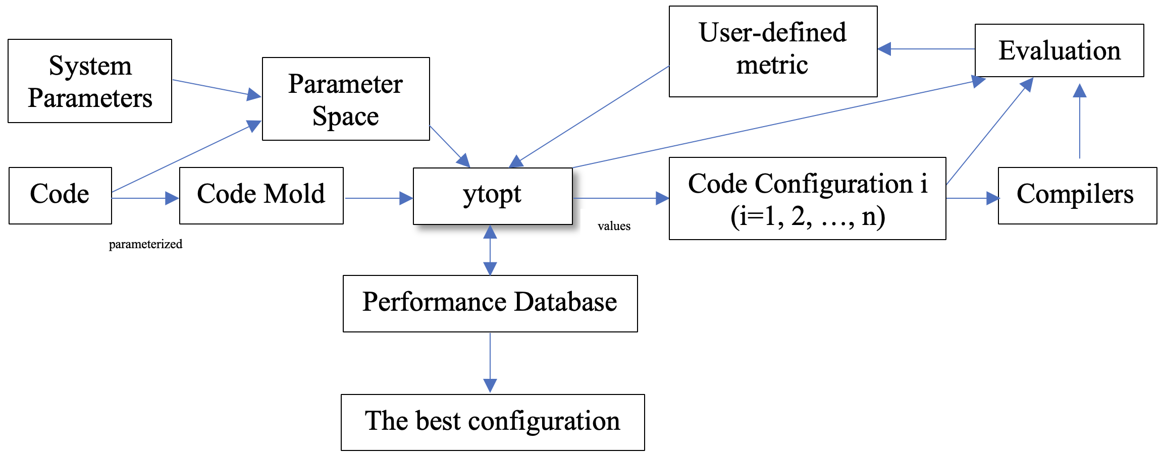
Figure 1: ytopt autotuning framework

Figure 1 presents the framework for autotuning various applications. The application runtime is the primary user-defined metric. We use ConfigSpace to analyze an application code in order to identify the important tunable application and system parameters needed to define the parameter space using ConfigSpace [ConfigSpace(2023)]. We use the tunable parameters to parameterize an application code as a code mold. ytopt starts with the user-defined parameter space, the code mold, and user-defined interface that specifies how to evaluate the code mold with a particular parameter configuration.

The search method within ytopt uses Bayesian optimization, where a dynamically updated random forest surrogate model that learns the relationship between the configurations and the performance metric is used to balance exploration and exploitation of the search space. In the exploration phase, the search evaluates parameter configurations that improve the quality of the surrogate model. In the exploitation phase, the search evaluates parameter configurations that are closer to the previously found high-performing parameter configurations. The balance is achieved through the use of the lower confidence bound (LCB) acquisition function that uses the surrogate model’s predicted values of the unevaluated parameter configurations and the corresponding uncertainty values. The LCB acquisition function is defined in Equation 1. For the unevaluated parameter configuration $x_{M}^{i}$, the trained model $M$ is used to predict a point estimate (mean value) $\mu(x_{M}^{i})$ and standard deviation $\sigma(x_{M}^{i})$.

$$a_{LCB}(x_{M}^{i})=\mu(x_{M}^{i})-\kappa\sigma(x_{M}^{i}),$$ (1)

where $\kappa\geq 0$ is a user-defined parameter that controls the trade-off between exploration and exploitation. When $\kappa=0$ for pure exploitation, a configuration with the lowest mean value is selected. When $\kappa$ is set to a large value ($>1.96$) for pure exploration, a configuration with large predictive variance is selected. The default value of $\kappa$ is 1.96. Then the model $M$ is updated with this selected configuration.

In our previous work [Wu(2023)] we autotuned four hybrid MPI/OpenMP ECP proxy applications—XSBench, AMG, SWFFT, and SW4lite—at large scales. We used Bayesian optimization with a random forest surrogate model to effectively search the parameter spaces with up to 6 million different configurations on Theta [Theta(2022)] at Argonne National Laboratory and Summit [Summit(2022)] at the Oak Ridge Leadership COmpouting Facility (OLCF). The experimental results showed that our autotuning framework had low overhead and good scalability. By using ytopt to identify the best configuration, we achieved up to 91.59% performance improvement, up to 21.2% energy savings, and up to 37.84% EDP improvement on up to 4,096 nodes.

Nevertheless, our current ytopt has several limitations. It evaluates one parameter configuration each time. This reduces the effectiveness of identifying the promising search regions at the beginning of the autotuning process because of having few data points for training the random forest surrogate model. This one-by-one evaluation process is also time-consuming. There is a need for ytopt to parallelize the multiple independent evaluations to accelerate the autotuning process. Some of initial randomly selected configurations may result in much larger execution time than the baseline as we had in [Wu(2023)]. There is also a need for ytopt to set a proper evaluation timeout in order to evaluate more good configurations. These are the main motivations for this work.

2.2 libEnsemble

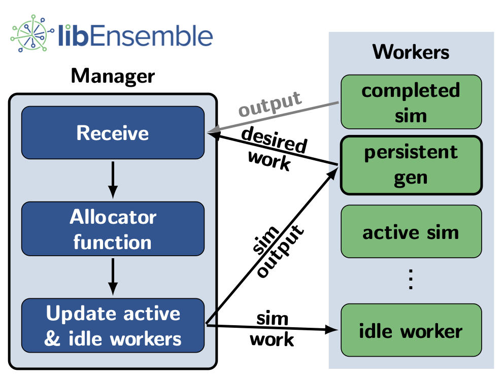
Figure 2: libEnsemble’s manager-worker paradigm: the manager allocates workload to multiple workers, which perform computations via user functions

libEnsemble [Hudson(2021), Hudson(2023)] is an advanced Python toolkit, developed under the ECP PETSc/TAO project [PETSC/TAO(2023)], designed to coordinate workflows of asynchronous, dynamic ensembles of calculations on massively parallel resources. Targeting complex design, decision-making, and inference problems, libEnsemble allows applications and studies where single instances typically do not scale to an entire machine to effectively harness high-performance computing environments.

One of the key strengths of libEnsemble is its extreme portability and scalability. It operates seamlessly across various computing platforms, from laptops to clusters to leadership-class machines. This flexibility ensures that the toolkit can be employed in a wide range of environments without extensive configuration or modification. Additionally, libEnsemble supports heterogeneous computing workflows, dynamically and portably assigning and reassigning CPUs, GPUs, or multiple nodes to tasks, making it an ideal solution for workflows using diverse computational resources.

libEnsemble employs a manager-worker paradigm, depicted in Figure 2, that significantly enhances its capability to handle dynamic and asynchronous calculation workflows. The manager and workers together coordinate three core plug-and-play components: simulation (sim) functions, generator (gen) functions, and allocator functions, all referred to as user functions. The simulation function is responsible for executing the individual calculations within the ensemble. These could range from complex simulations to simpler data-processing tasks. The generator function plays a crucial role in deciding the next set of calculations to be performed, often based on the results of previous simulations. Generators can adjust the direction of the computational workflow dynamically, ensuring that the ensemble is always computing on the most relevant and promising tasks. The allocator function decides what tasks are given to which workers based on the current state of the ensemble and the available resources. This modular approach allows libEnsemble to dynamically adjust its focus based on intermediate results. Such flexibility is key to efficiently navigate large, complex computational spaces.

libEnsemble also includes advanced features to automatically monitor running calculations and manage data-flow between tasks, which enhances libEnsemble’s utility in complex studies where intertask communication is crucial. At a baseline, simple send and receive methods are available to ensemble members to send intermediate data and hyperparameters to each-other via the manager. From this foundation, a critical capability includes cancelling or preempting application instances, as directed by an autotuning or other decision process, providing scientists with more efficient control over the study.

Another significant advantage of libEnsemble is its low start-up cost for domain scientists, regardless of their familiarity with parallel computing. It requires no additional background services or processes to function, making it straightforward to integrate and deploy in various computational environments. This ease of setup, combined with its powerful features, positions libEnsemble as a highly versatile and user-friendly toolkit for coordinating workflows in high-performance computing environments. The complete documentation of libEnsemble is presented in [Hudson(2024)]; examples of diverse applications of libEnsemble are demonstrated in [Chang(2020), Neveu(2019), Ferran Pousa(2019)].

3 Integrated Autotuning Framework ytopt-libe in Performance and Energy

In this section we discuss the integration of the ytopt autotuning framework and libEnsemble, and we use the framework ytopt-libe to autotune OpenMC on ORNL Crusher using metrics such as the application FoM, application runtime, energy, and EDP, where the application FoM is the primary performance metric. Energy consumption captures the trade-off between the application runtime and power consumption; and EDP captures the trade-off between the application runtime and energy consumption.

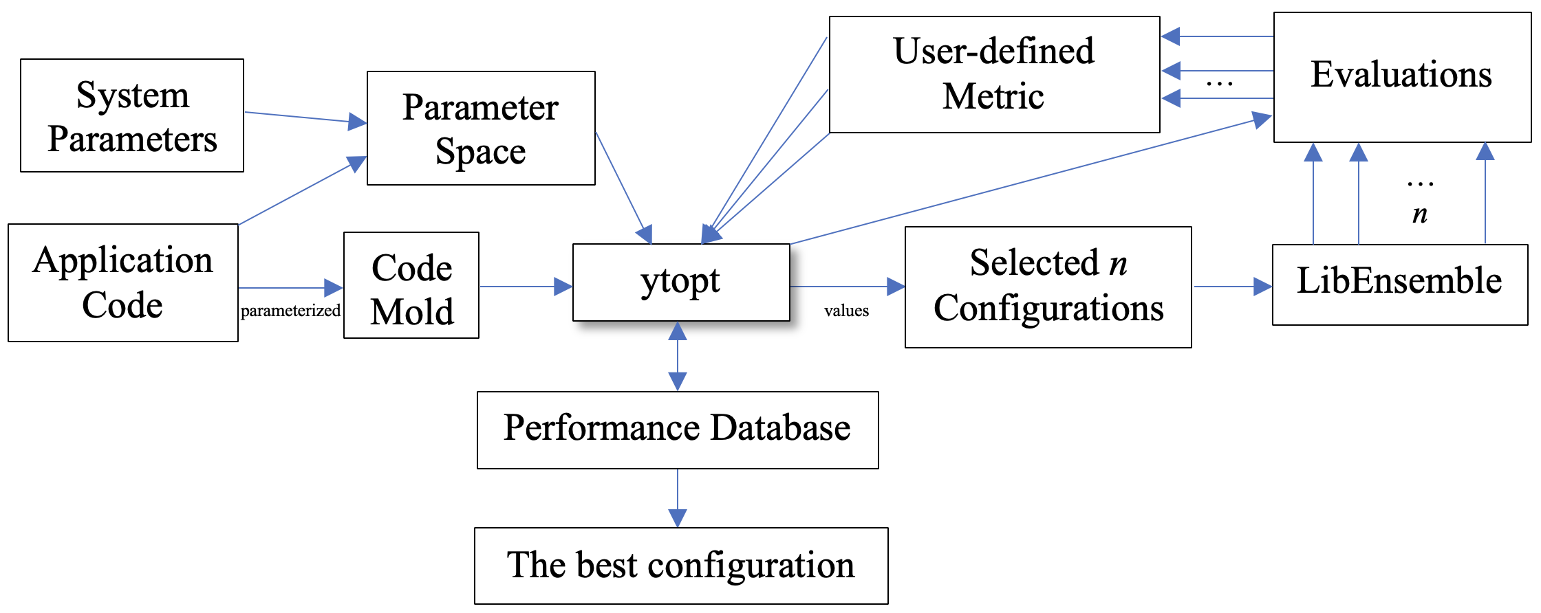
Figure 3: Integrated autotuning framework ytopt-libe

Figure 3 presents the framework ytopt-libe for autotuning various applications in user-defined metrics. We analyze an application code to identify the important tunable application and system parameters (OpenMP environment variables and number of MPI ranks per GPU) to define the parameter space using ConfigSpace. We use these tunable parameters to parameterize an application code/script as a code mold. ytopt-libe starts with the user-defined parameter space, the code mold, and user-defined interface that specifies how to evaluate the code mold with a particular parameter configuration.

For the integration of ytopt and LibEnsemble, the generator function in libEnsemble uses the ytopt’s Bayesian optimization with random forest surrogates to drive the ensemble of calculations, the simulation function is the evaluation of the ExaSMR application calculation, and the allocation function uses the libEnsemble default for a persistent worker operating in batch mode. Upon initialization, a worker is dedicated to running the persistent generator. For this case, batch behavior is desired, so the allocation function tells the generator to produce a point to evaluate for each of the remaining idle workers. The allocation function dispatches these points out; and once all of these simulation runs are completed, the persistent generator is informed of the results, and the process is repeated.

The iterative phase of the proposed autotuning framework ytopt-libe has the following steps:

• libEnsemble creates one manager and $n$ independent workers specified by a user.

• Bayesian optimization selects $n$ parameter configurations for evaluation .

• The code mold is configured with each selected configuration to generate new code for each worker in parallel.

• For each worker, based on the value of the number of threads in each configuration, the number of nodes reserved, and the number of MPI ranks, the job command line using srun/mpirun for the launch of the application on the compute nodes is generated in parallel.

• Each new code is compiled with other codes needed to generate an executable in parallel for each worker (if needed).

• For each worker, the generated command line is executed to evaluate the application with the selected parameter configuration in parallel; each result is sent back to the ytopt and is recorded in the performance database in an asynchronous and dynamic way: (1) All workers are independent; there is no communication among them. (2) When a worker finishes an evaluation, it sends its result back to the ytopt; then the ytopt updates the surrogate model and selects a new configuration for the worker to evaluate (Step 1).

Steps 1–5 are repeated until the maximum number of code evaluations or the wall-clock time is exhausted for the autotuning run.

In this way, the proposed autotuning framework ytopt-libe not only accelerates the evaluation process of ytopt to take advantage of massively parallel resources but also improves the accuracy of the random forest surrogate model by feeding more data for more efficient search.

To set a proper evaluation timeout in order to evaluate more good configurations, ytopt requires the timeout value as a user input. The basic principle is based on the baseline application runtime plus some overhead. Therefore, the typical timeout setting is 1.5 times the baseline runtime. ytopt uses Python subprocess.Popen.communicate [subprocess(2022)] to terminate an evaluation process after timeout and sets the timeout as the returned objective value for ytopt to record the value and the configuration in the performance database. Then ytopt searches the next configuration for evaluation.

4 OLCF Frontier TDS System Crusher

The Crusher [Crusher(2023)] system has identical hardware and similar software to those of the Frontier system at OLCF. Crusher has 2 cabinets, the first with 128 compute nodes and the second with 64 compute nodes, for a total of 192 compute nodes.

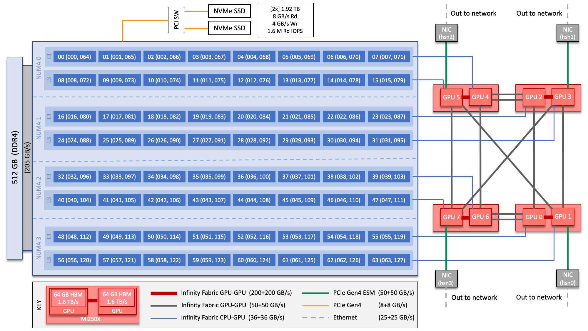
Figure 4: Crusher node diagram [Crusher(2023)].

As shown in Figure 4, each Crusher compute node consists of one 64-core AMD EPYC 7A53 “Optimized 3rd Gen EPYC” CPU with 2 hardware threads per core with access to 512 GB of DDR4 memory. Each node also contains four AMD MI250X, each with 2 Graphics Compute Dies (GCDs) for a total of 8 GCDs per node. The CPU is connected to each GCD via Infinity Fabric CPU-GPU, allowing a peak host-to-device and device-to-host bandwidth of 36+36 GB/s. The 2 GCDs on the same MI250X are connected with Infinity Fabric GPU-GPU with a peak bandwidth of 200 GB/s. The GCDs on different MI250X are connected with Infinity Fabric GPU-GPU, where the peak bandwidth ranges from 50 to 100 GB/s based on the number of Infinity Fabric connections between individual GCDs. We refer to the GCDs simply as GPUs in this paper. Slurm [Slurm(2022)] is the workload manager used to interact with the compute nodes on Crusher; srun is used to launch application jobs on Crusher’s compute nodes in Slurm.

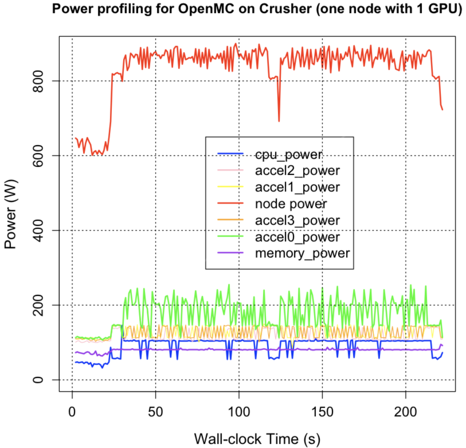
Figure 5: Power profiling for a single GPU using APEX on Crusher

We use APEX [APEX(2023)] to read the Cray pm_counters to obtain the power consumptions for each node and its components, such as CPU, GPUs, and memory. For instance, Figure 5 shows the power profiling over time for OpenMC using APEX, where one of the GPUs from accelerator 0 was used for running the OpenMC and other accelerators are idle; there are also some activities in the CPU and a few activities in memory for this application.

5 ECP Application OpenMC and Its Parameter Space

5.1 ECP Application OpenMC

OpenMC [Romano(2015)] is a community-developed Monte Carlo neutral transport code. Recent years have seen development and optimization of the code for GPUs via the OpenMP target offloading model, as part of the ECP ExaSMR project [ExaSMR(2023)]. The goal of the ExaSMR project was to simulate small modular nuclear reactors in high fidelity using a multiphysics approach that coupled Monte Carlo neutron transport with computational fluid dynamics. OpenMC has so far demonstrated excellent performance across a variety of GPU architectures, including Intel, NVIDIA, and AMD [Tramm(2022)]. While OpenMC’s portability is a great benefit for its users, however, fully fine-tuning the code for each GPU architecture by hand is impractical. Rather, an automated approach is desired so as to find optimal parameters for each new system and to determine whether they tend to differ between systems or whether a common default can be used everywhere.

In this study we perform tuning and analysis with OpenMC on a standard reactor physics benchmark simulation problem—the Hoogenboom–Martin (HM) “large” variant [Hoogenboom(2011)] representing a depleted fuel reactor with 272 nuclides in total. Optimal performance parameters discovered when tuning for this problem are expected to translate directly to a wide variety of fission reactor simulation problems, including the ExaSMR challenge problem.

Table 1: OpenMC tunable parameters

Parameter	Type	Range/Bounds	Default
Maximum number of particles in-flight	Integer	100k - max that will fit in memory ($\sim$ 8 million)	1 million
Number of MPI ranks per GPU	Integer	1 - 4	1
Number of logarithmic hash grid bins	Integer	100 - 100k	4,000
Queuing logic type	Mode	Queued vs. Queueless	Queued
Minimum sorting threshold (queued mode only)	Integer	0 (always sort) - infinity (never sort)	20,000

The tunable parameters and their ranges of OpenMC with the HM Large benchmark problem are shown in Table 1. A description of each parameter is given below.

• The maximum number of particles in-flight parameter controls the number of particles that are allowed to be alive at any one point in time. This parameter does not affect the numerical characteristics of the simulation, since the user is still allowed to select any number of particle histories per simulation batch. If the number of particles allowed in-flight is below the number of particles per batch selected by the user, then the particle buffer will be refilled dynamically after each kernel call to replace any particles that have reached their termination criteria, until all particle histories have been simulated in the batch. The motivating reason for this parameter is both to control memory usage (since particle objects are relatively large) and to allow for more optimal kernel work sizes to be selected. Based on our experience, the maximum number of particles in-flight is in the range of 100,000 and $\sim$ 8 million, with the default of 1 million.

• The number of MPI ranks per GPU parameter is useful since some architectures see significant performance gains when multiple MPI ranks are launched per GPU, in effect resulting in multiple streams running on the GPU concurrently. This variable is correlated with others in that selection of a higher number of MPI ranks will greatly reduce the memory available to each rank, which constrains selection of other parameters that involve an increased usage of memory. We need to tune the parameter to identify the proper number of MPI ranks per GPU for the best performance.

• The number of logarithmic hash grid bins is a tunable parameter that affects performance of the most expensive kernel in OpenMC for depleted nuclear reactor simulations—the macroscopic cross-section lookup kernel. This parameter determines how many logarithmic hash bins the energy space is divided into. If only a single bin were to be selected, then each nuclide in a given material in the simulation would need to be searched for data that corresponds to the neutron’s current energy at each stage of the simulation. For depleted fuel materials, this results in hundreds of separate binary search operations per macroscopic lookup. If a very high number of hash bins are selected, then all search operations can be eliminated and replaced with direct access operations. While a choice of a very high number of grid bins is often much faster, it comes at the cost of impractically high memory usage requirements. Thus, there is an inherent balance between memory usage and speedup that can result in architecture-specific tuning of this parameter. Choices resulting in high memory usage may also reduce the number of particles in-flight that are possible, making this variable somewhat correlated to others that result in more memory pressure.

• The queuing logic parameter selects between two different control flow implementations. The queued method involves the host maintaining discrete queues of particles representing each event type in the simulation. The host selects which kernel to launch on the device based on which queue has the most particles in it. This sort of dynamic queuing is useful given the stochastic nature of the Monte Carlo transport process. A result of this policy is that the number of particles in each queue must be transmitted back to the host, potentially increasing kernel invocation overhead and creating bubbles when kernel runtimes are very low. The second option, the queueless mode, uses simpler logic on the host that just loops over all event types until all particles have terminated. This eliminates the need to transfer any particle count data between the host and the device after each kernel invocation, potentially reducing overhead, but at the loss of having to subscribe threads for particles that do not need that event. Such threads simply check whether their particle requires the event and return immediately if the kernel is not needed, potentially resulting in inefficient thread divergence.

• The minimum sorting threshold parameter sets a limit on the number of particles that must be present in a queue to undergo sorting. Below this limit, no sorting is performed. The sorting operation improves memory locality of cross-section lookup operations by ensuring that adjacent particles in the buffer are located in the same material and close in energy. If many particles are in-flight and sorting is performed, potentially all threads within a workgroup (block) may be accessing the same data. However, if there are very few particles in-flight, then sorting may not result in any meaningful improvements in locality because threads may be accessing data that is no longer on the same cache line. In this case, the cost of the sorting operation may outweigh the benefits, so a minimum threshold parameter is useful for tuning.

5.2 Parameter Space for OpenMC

Based on the tunable application parameters in Table 1 and the system parameters such as the number of threads and OpenMP thread placement, we define the parameter space for OpenMC using ConfigSpace as follows.

cs = CS.ConfigurationSpace(seed=1234)
# queuing logic type
P0 = CSH.CategoricalHyperparameter(name=’P0’, choices=
["openmc", "openmc-queueless"], default_value="openmc")
# maximum number of particles in-flight (option -i)
P1= CSH.UniformIntegerHyperparameter(name=’P1’, lower=100000,
upper=8000000, default_value=1000000, q=1000)
# number of logarithmic hash grid bins (option -b)
P2 = CSH.UniformIntegerHyperparameter(name=’P2’, lower=100,
upper=100000, default_value=4000, q=100)
# minimum sorting threshold (option -m)
P3 = CSH.UniformIntegerHyperparameter(name=’P3’, lower=0,
upper=1000000, default_value=20000, q=1000)
#number of threads
P4= CSH.UniformIntegerHyperparameter(name=’P4’, lower=2,
upper=8, default_value=8)
#number of tasks per gpu
P5= CSH.OrdinalHyperparameter(name=’P5’,sequence=[1, 2],
default_value=1)
# omp placement
P6= CSH.CategoricalHyperparameter(name=’P6’, choices=
[’cores’,’threads’,’sockets’], default_value=’threads’)
cs.add_hyperparameters([P0, P1, P2, P3, P4, P5, P6])

cond = EqualsCondition(P3, P0, "openmc")
cs.add_conditions([cond])

Here P0 is the queuing logic type parameter with the choices of “openmc” (queued OpenMC code) and “openmc-queueless” (queueless OpenMC code); P1 is the maximum number of particles in-flight with the command line option -i; P2 is the number of logarithmic hash grid bins with the command line option -b; P3 is the minimum sorting threshold for only queued OpenMC code with the command line option -m; P4 is the number of OpenMP threads per task; P5 is the number of MPI tasks per GPU; and P6 is the OpenMP thread placement type, which may impact the OpenMP performance. The default values are set based on the application and system default settings, so the default configuration is the starting point for autotuning. Notice that there is some dependency among these parameters. The ConfigSpace condition statement EqualsCondition(P3, P0, “openmc”) means that making P3 is an active hyperparameter if P0 has the value “openmc”; otherwise, P3 has the empty value “nan.” P4 depends on P5 because each core of a 64-core AMD EPYC CPU supports two hardware threads, with a total of 128 threads per node. Using 2 MPI tasks per GPU means 16 MPI tasks per node, so the number of threads P4 is at most 8.

The hybrid MPI/OpenMP offload OpenMC code is written in C++, MPI, and OpenMP offloading (version: June 10, 2022) and is very complex; its compiling time is very long. We precompile OpenMC to two executables: openmc and openmc-queueless. Because these application parameters for OpenMC are command line parameters, we can avoid the compiling and just pass these parameters to the OpenMC executable.

We parameterize the OpenMC command line and its options and define the code mold (openmc.sh) as follows.

#!/bin/bash
pp0="#P0"
pp="openmc"
if [ "$pp0" = "$pp" ]
then
        openmc  --event -i #P1 -b #P2 -m #P3
else
        openmc-queueless --event -i #P1 -b #P2
fi

Here OpenMC uses event-based parallelism with the option ”–event” for both queued and queueless modes. P3 is only for the queued OpenMC.

We use the script to pass the parameters P4, P5. and P6 to the srun command with the following command line options.

-c #P4
--ntasks-per-gpu=#P5
--cpu-bind=#P6

After ytopt-libe selects a configuration, the parameters are replaced with the selected values in the code mold for evaluation.

6 Autotuning in Performance

In this section we apply the proposed framework ytopt-libe, shown in in Figure 3, to autotune the performance of OpenMC. The performance metric is the figure of merit, which is the rate to process the number of particles per second. Slurm’s srun is used to launch an application to compute nodes on OLCF Crusher. The CPU processor core on Crusher supports the simultaneous multithreading level of 2 as default so that the number of threads per node is supported up to 128.

As shown in Figure 3, ytopt-libe creates one manager and $n$ independent workers specified by a user, and Bayesian optimization in ytopt-libe selects $n$ parameter configurations for evaluation. Based on the value of the number of threads from the selected configuration, the number of nodes reserved, and the number of MPI ranks, ytopt generates the srun command line for application launch on compute nodes.

For the experimental setup, we set the total number of evaluations to 256 for all experiments and run each worker on the dedicated node(s). We use the following terms in the rest of this paper. $(1GPU,1node)$ stands for using 1 GPU on a single node. $(8GPUs,1node)$ stands for using 8 GPUs on a single node. $(2workers,1GPU/n)$ means that each work runs on 1 GPU on a single dedicated node with the total 2 nodes used for 2 workers. $(4workers,8GPUs/n)$ means that each work runs on 8 GPUs on a single dedicated node with the total 4 nodes used for 4 workers. $(4workers,8nodes)$ means that each worker runs on 2 nodes with 8 GPUs/n and the total 8 nodes. Notice that each worker is assigned to one or more dedicated nodes so that its performance is not impacted by other workers.

In this paper the baseline performance measurement is the default values for application parameters for both queueless and queued modes with the default system environment settings. We use OpenMC with the HM-Large benchmark problem. We run both modes (queueless, queued) with the default application settings on the default system environment of Crusher five times and use the largest particles/s as the baseline for performance comparison.

6.1 Performance Comparison

In this subsection we compare the performance using ytopt itself and the proposed framework ytopt-libe in the following two ways:

• Investigate how ytopt-libe accelerate the autotuning evaluations.

• Explore what is the proper number of workers to use for identifying the best configuration (varying the number of workers from 2 to 16).

Figure 6 shows autotuning OpenMC over time on a single GPU using ytopt, where the red line stands for the baseline performance and the blue circle is the FoM for a selected configuration evaluation. Over time, ytopt leads to the high-performing regions of the parameter space, which result in much better performance than that of the baseline performance. However, several initial configurations had a timeout termination so that its performance was set very low with a constant negative value by ytopt. In this way, the timeout configurations were marked as the worst regions so that the next search would avoid these regions. Using ytopt took 27,401 s to finish just 128 of 256 evaluations because of the large application runtimes (more than 200 s). ytopt identified the best configuration, which resulted in 27.68% performance improvement.

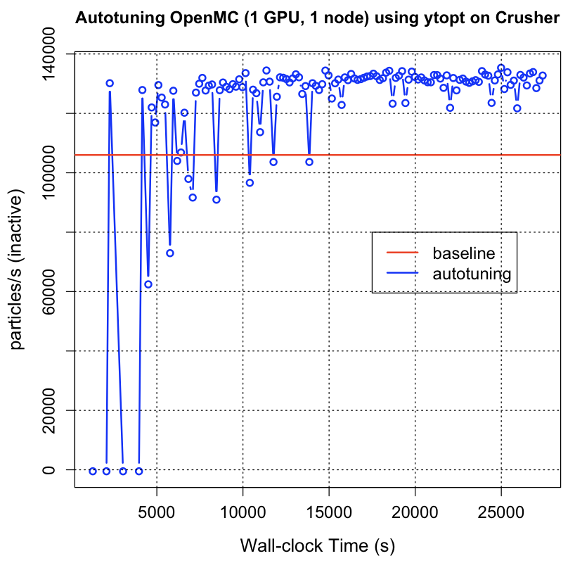
Figure 6: Autotuning OpenMC on a single GPU using ytopt

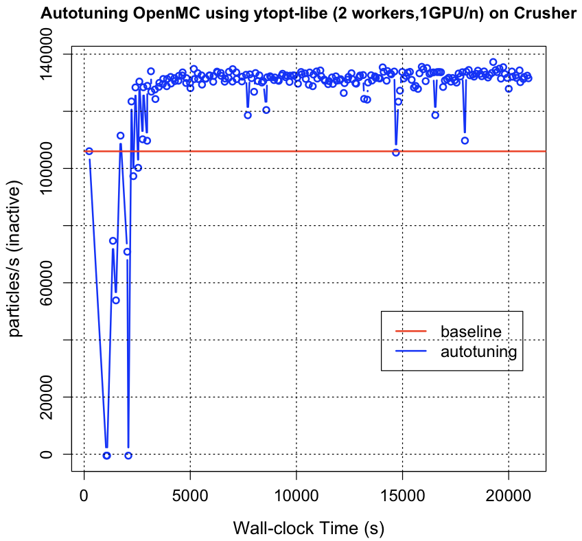
Figure 7: Autotuning OpenMC on a single GPU using ytopt-libe with 2 workers

When ytopt-libe with 2 workers on two nodes is used to autotune OpenMC on a single GPU, as shown in Figure 7, ytopt-libe creates two independent workers and selects two configurations: one worker runs the OpenMC with one configuration on a single GPU of one node, and the other worker runs the OpenMC with the other configuration on a single GPU of another node. In this way, two evaluations are executed independently in parallel. It took 20,931 s to finish 256 evaluations, reducing the overall autotuning time for using ytopt by more than a half. ytopt-libe identified the best configuration, which resulted in 29.48% performance improvement.

Can we use as many workers as possible for ytopt-libe to autotune OpenMC? To answer this question, we vary the number of workers from 2 to 16 to explore what is the best number of workers to use for identifying the best configuration.

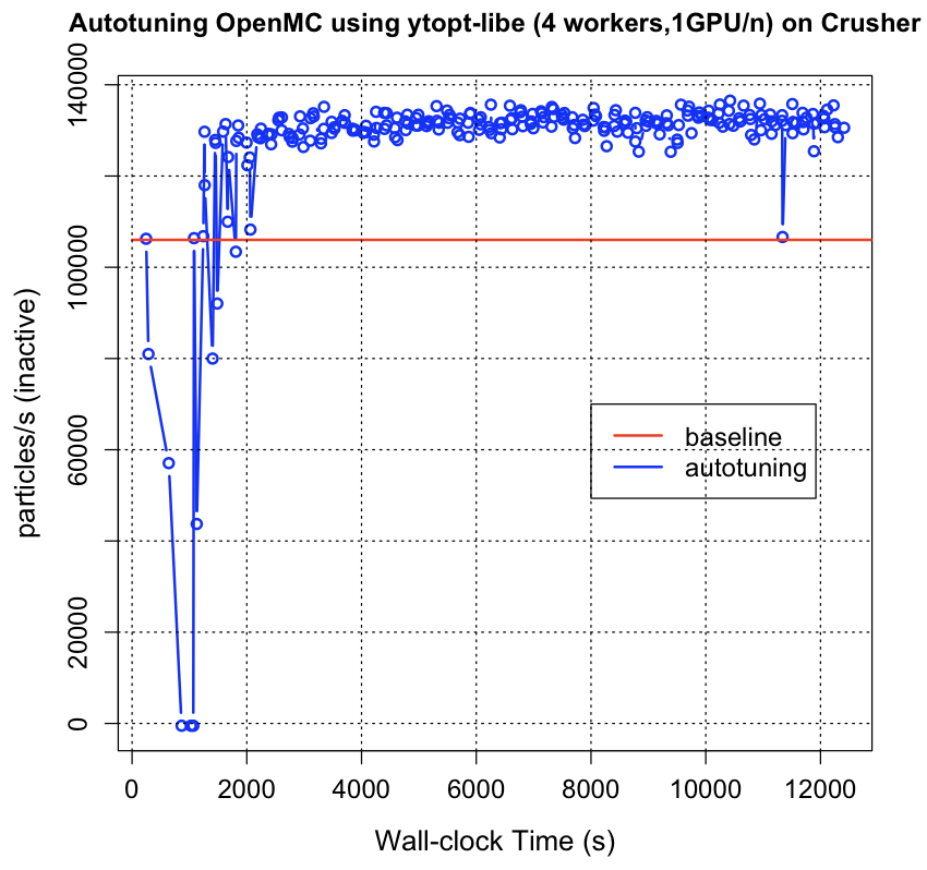
Figure 8: Autotuning OpenMC on a single GPU using ytopt-libe with 4 workers

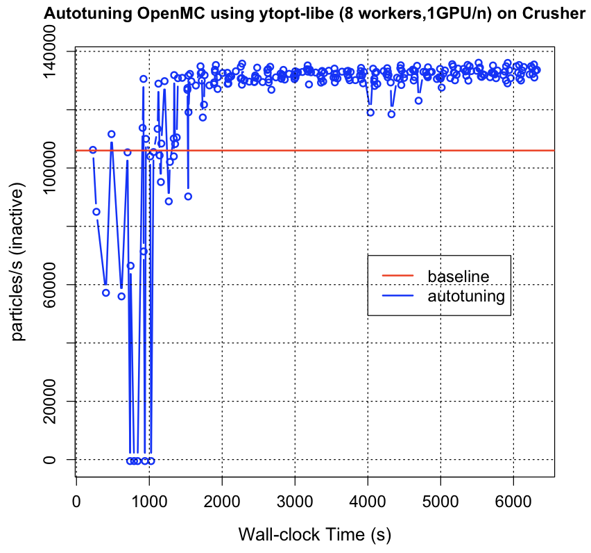
Figure 9: Autotuning OpenMC on a single GPU using ytopt-libe with 8 workers

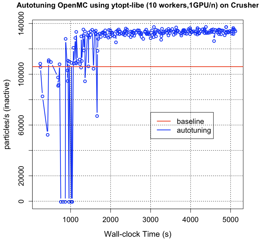
Figure 10: Autotuning OpenMC on a single GPU using ytopt-libe with 10 workers

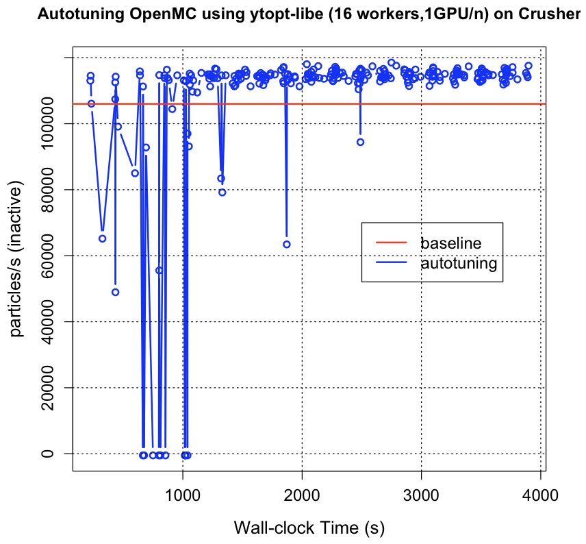
Figure 11: Autotuning OpenMC on a single GPU using ytopt-libe with 16 workers

Table 2: Performance improvement comparison (based on the baseline) using ytopt and ytopt-libe with different number of workers

Method	Number of evaluations	Performance improvement (%)	Total autotuning time (s)
ytopt	128 of 256	27.68	27,401
ytopt-libe with 2 workers	256	29.48	20,931
ytopt-libe with 4 workers	256	28.79	12,411
ytopt-libe with 8 workers	256	28.39	6,320
ytopt-libe with 10 workers	256	29.49	5,119
ytopt-libe with 16 workers	256	11.81	3,897

Similarly, to autotune OpenMC on a single GPU per node with a total of 256 evaluations, we conduct the following experiments. We configure ytopt-libe to use 4 workers on 4 nodes in Figure 8, 8 workers on 8 nodes in Figure 9, 10 workers on 10 nodes in Figure 10, and 16 workers on 16 nodes in Figure 11. Table 2 summarizes the performance improvement comparison using ytopt and ytopt-libe with different numbers of workers on Crusher. We observe that ytopt-libe significantly reduces the time spent in the ytopt autotuning process and that ytopt-libe with 10 workers resulted in the best performance improvement, 29.49%. Using larger numbers of workers, however, does not achieve the best performance improvement. Especially for the case of ytopt-libe with 16 workers, the performance improvement significantly decreases to just 11.81%. The reason is as follows. When ytopt-libe used 16 workers, it selected 16 configurations to start evaluation at the beginning of the autotuning process. Unfortunately, more bad configurations were selected for the evaluation, as shown in Figure 11. These data points were fed to the random forest surrogate model, causing a less accurate model. This results in an inefficient search for the next configurations. Therefore, we have to deal with the trade-off among the runtime, performance improvement, and number of available compute resources.

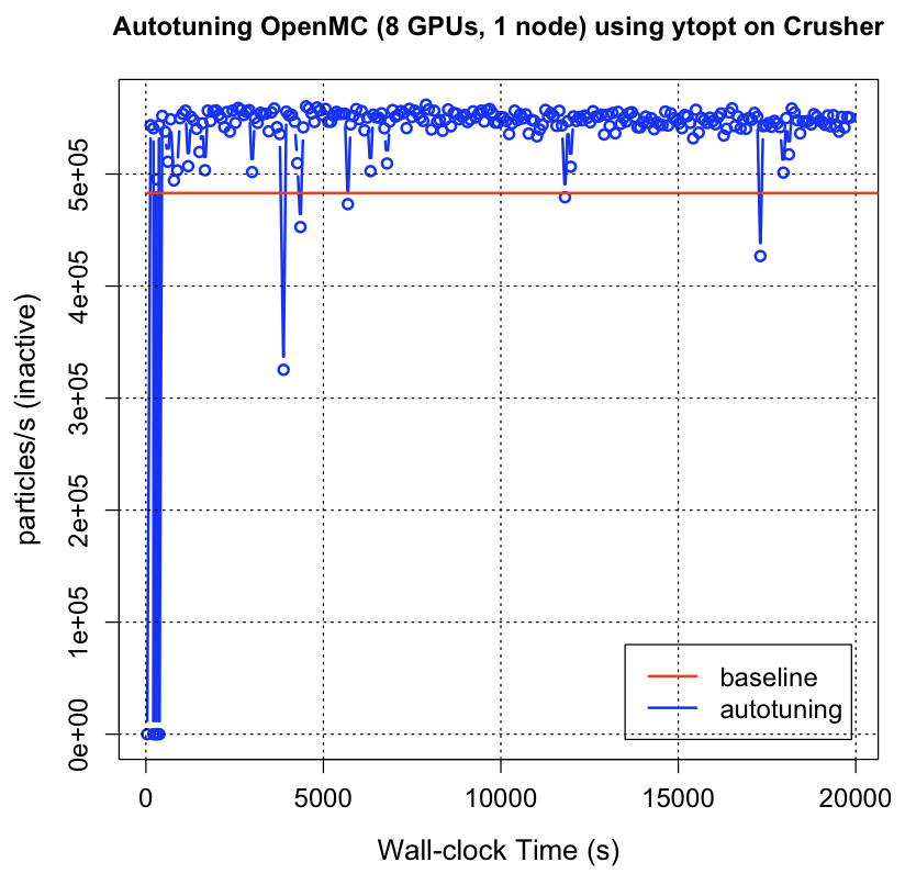
Figure 12: Autotuning OpenMC on 8 GPUs using ytopt

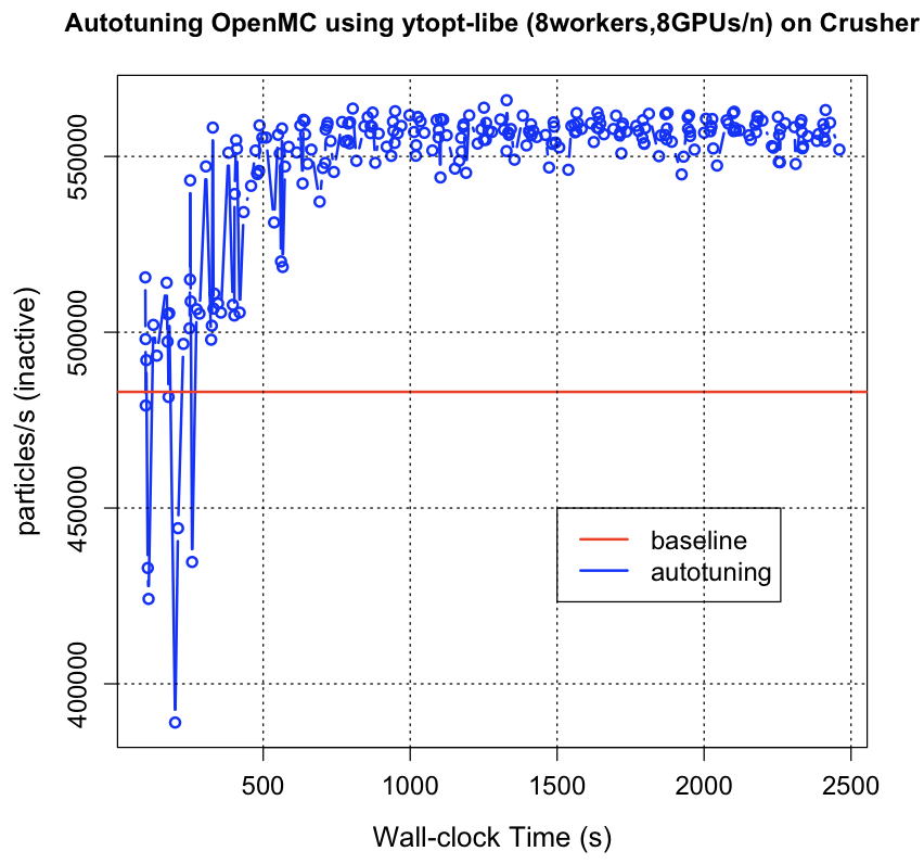
Figure 13: Autotuning OpenMC on 8 GPUs using ytopt-libe

Figure 12 shows autotuning OpenMC over time on 8 GPUs on a node using ytopt. Over time, ytopt leads to the high-performing regions of the parameter space, which results in much better performance than the baseline performance. It took 19,631 s to finish 256 evaluations. ytopt identified the best configuration, which resulted in 16.33% performance improvement. Notice that using 8 GPUs per node for OpenMC resulted in much higher FoM than using 1 GPU per node in Figure 6. Figure 13 shows autotuning OpenMC over time on 8 GPUs of a node using ytopt-libe with 8 workers. This significantly reduced the total ytopt autotuning time by almost eight times and also achieved 17.17% performance improvement. Using ytopt-libe with different numbers of workers for the 8 GPUs per node cases, we found that the trend was similar to that for the 1 GPU per node cases, as shown in Table 2.

6.2 Performance Scaling Analysis

In this subsection we investigate the application performance scaling using ytopt-libe. For the analysis, we use a constant number of workers, 4, and explore the performance impacts when each worker runs OpenMC on 1, 2, 4, 8, and 16 nodes with 8 GPUs per node. Because Crusher has a total of 192 nodes, if we choose more than 4 workers (e.g., 8, 10, or 16), there are not enough available compute nodes for using ytopt-libe.

Figure 14 shows autotuning OpenMC on 8 GPUs using ytopt-libe with 4 workers on 4 nodes with 8 GPUs per node. Over time, ytopt-libe leads to the high-performing regions of the parameter space, which results in much better performance than the baseline performance and identifies the best configuration, which results in 16.41% performance improvement.

Similarly, to autotune OpenMC on different numbers of GPUs with 256 evaluations, we conduct the following experiments. We configure ytopt-libe to run with 4 workers on 8 nodes (Figure 15), on 16 nodes (Figure 16), on 32 nodes (Figure 17), and on 64 nodes (Figure 18). Table 3 summarizes the performance improvement comparison using topt-libe with 4 workers and different numbers of GPUs on Crusher. We observe that ytopt-libe identifies the best configuration, which results in at least 11.03% performance improvement. However, the scalablity of OpenMC from 8 GPUs to 128 GPUs is limited because the design for the version of OpenMC mainly focuses on the single-GPU performance.

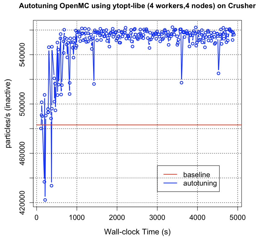
Figure 14: Autotuning OpenMC on 8 GPUs using ytopt-libe

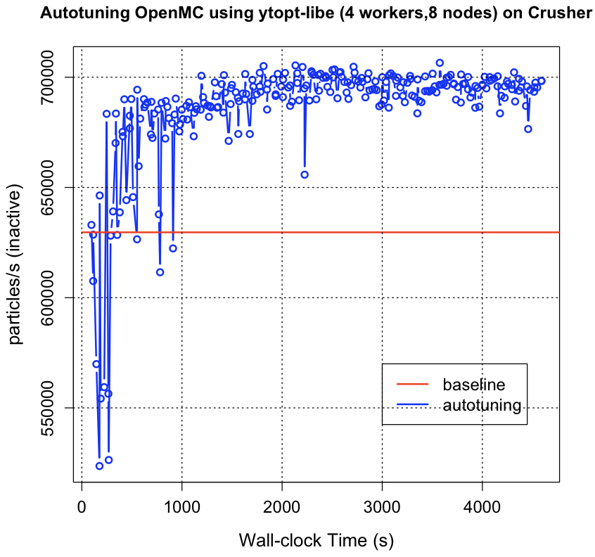
Figure 15: Autotuning OpenMC on 16 GPUs using ytopt-libe

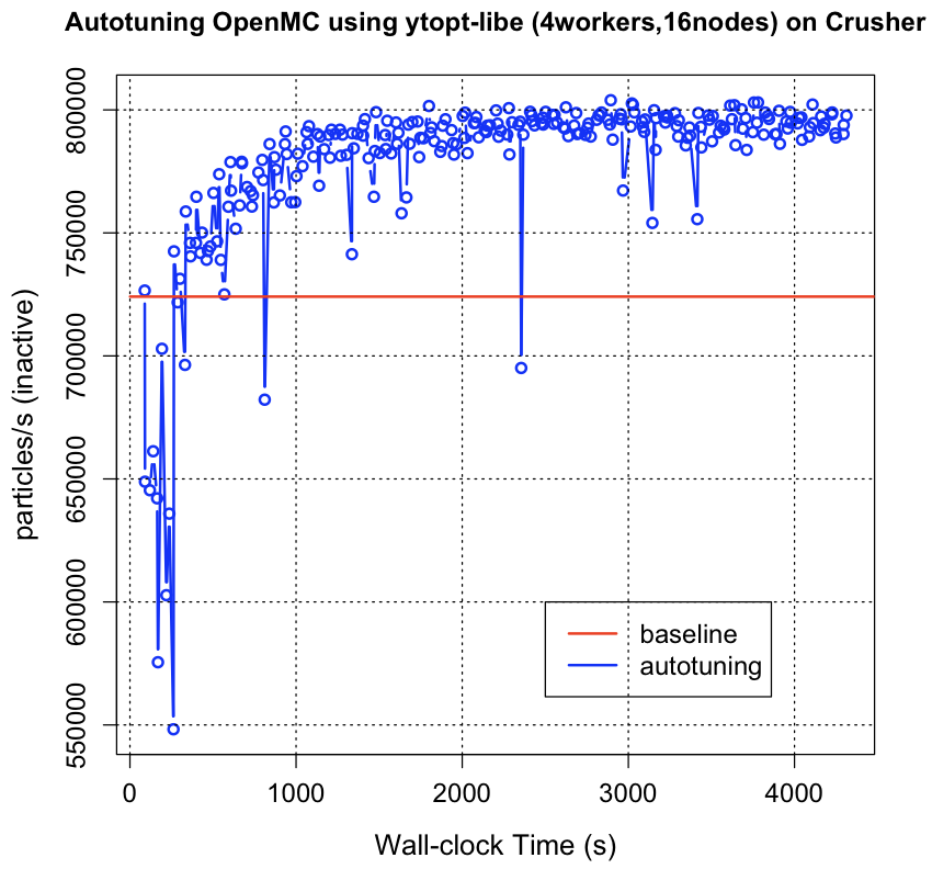
Figure 16: Autotuning OpenMC on 32 GPUs using ytopt-libe

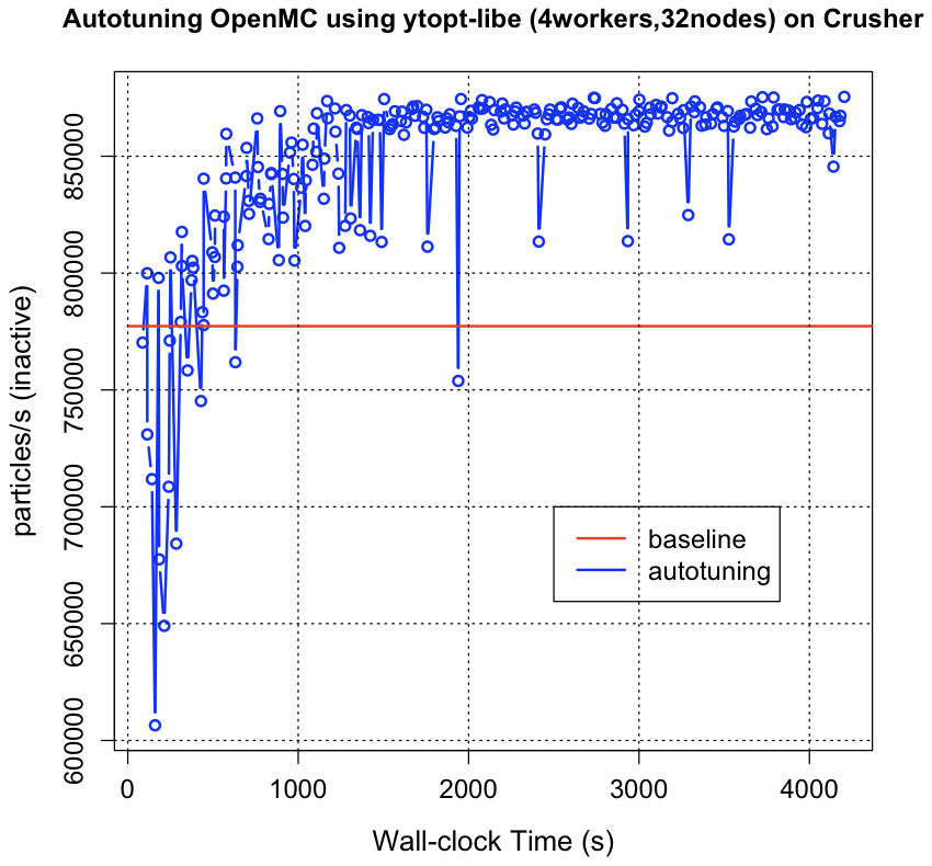
Figure 17: Autotuning OpenMC on 64 GPUs using ytopt-libe

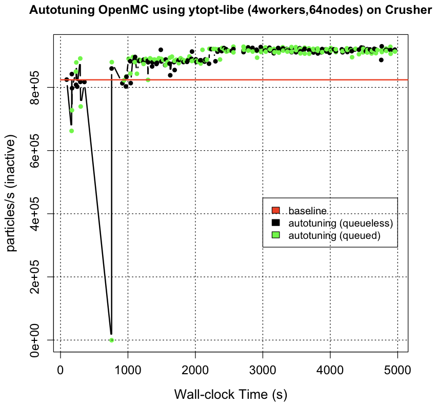
Figure 18: Autotuning OpenMC on 128 GPUs with queued and queueless using ytopt-libe

Table 3: Performance improvement for OpenMC on different numbers of GPUs using ytopt-libe with 4 workers

Number of GPUs	Baseline Performance (Particles/s)	Best Performance (Particles/s)	Performance improvement (%)
8	483033	562288	16.41
16	629647	706535	12.21
32	724098	803931	11.03
64	777287	875419	12.62
128	823997	930078	12.87

Figure 18 shows autotuning OpenMC on 8 GPUs using ytopt-libe with 4 workers on 64 nodes with 8 GPUs per node. Over time, ytopt-libe leads to the high-performing regions of the parameter space, which results in much better performance than the baseline performance and identifies the best configuration, which results in 12.87% performance improvement. However, OpenMC with one configuration had a timeout termination. so that one negative value was assigned by ytopt-libe as the worst parameter space region. In this figure we split the overall autotuning process into two parts: one with the color green for OpenMC with the queued mode and the other with the color black for OpenMC with the queueless mode. We observe that in the high-performing regions of the parameter space, using OpenM with the queued or queueless mode does not impact the performance much.

7 Autotuning in Runtime, Energy, and EDP

In the preceding section the results are all for FoM (particles/s) as the performance metric. What about other performance metrics? Application runtime (without the initialization time) is used to calculate the rate particles/s for FoM. Energy captures the trade-off between power consumption and runtime: it is the product of power and runtime. The energy delay product captures the trade-off between energy and runtime. It is the product of energy and runtime and the product of power and square of runtime. In this section we apply the proposed autotuning framework ytopt-libe in Figure 3 to autotune the application runtime, energy, and EDP of OpenMC on Crusher. We use the autotuning framework to explore the trade-offs for the application’s efficient execution with these performance metrics.

For measuring the baseline energy for each application executed on 8 GPUs on a single node, we use APEX [APEX(2023)] to run the application under the default system configuration five times. Then we use the smallest runtime/energy as the baseline runtime/energy. Figure 19 shows the power profiling for OpenMC with the default application settings on 8 GPUs using APEX. Comparing this figure with Figure 5, we can see that the default settings are not sufficient for efficient execution on 8 GPUs. Loading the HD5 datasets takes more 70 s and is the performance bottleneck as well.

Figure 19: Power profiling for 8 GPUs using APEX on Crusher

For autotuning energy and EDP, after the evaluation of a configuration APEX generates a summary report that records the package energy and DRAM energy for each node. We accumulate these values as the node energy. When ytopt receives the report from APEX, it calculates an average node energy and EDP and uses the average energy or EDP as the primary metric for autotuning.

Figure 14 shows autotuning OpenMC in FoM on 8 GPUs using ytopt-libe with 4 workers on 4 nodes with 8 GPUs per node. For the sake of simplicity, we use the same settings to autotune OpenMC in runtime, energy, and EDP on 8 GPUs using ytopt-libe with 4 workers on 4 nodes. Figure 20 presents autotuning OpenMC with the performance metric runtime on 8 GPUs using ytopt-libe. We observe that over time ytopt-libe leads to the high-performing regions of the parameter space, which results in much better runtime than that of the baseline and identifies the best configuration, which results in 17.05% performance improvement.

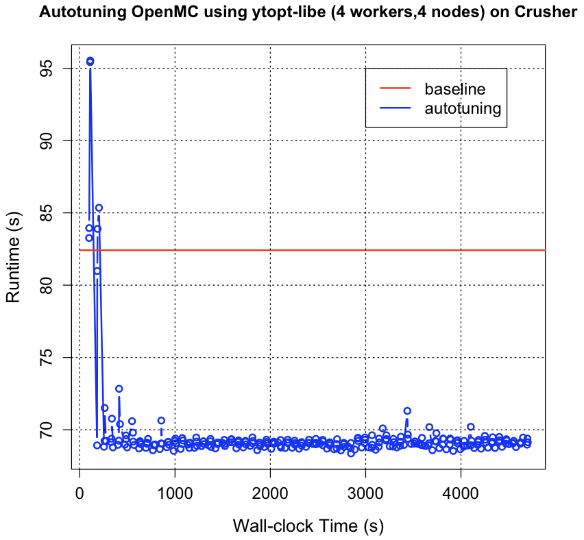
Figure 20: Autotuning OpenMC with the performance metric runtime on 8 GPUs using ytopt-libe

Figure 21 shows autotuning OpenMC with the performance metric energy on 8 GPUs using ytopt-libe. Although ytopt-libe identifies the best configuration, which results in 17.93% energy improvement, we observe that the energy pattern over time is not approximate to one good point. This is very different from Figure 20 where the runtime pattern is approximate to the best point with very little margin. This indicates that when ytopt-libe used four different nodes to run 4 evaluations for OpenMC in parallel, the power measurement for each node was varied significantly so that the energy consumption for each node had a larger difference.

Further, when we use ytopt-libe to autotune OpenMC with the performance metric EDP in Figure 22, ytopt-libe identifies the best configuration, which results in 30.44% EDP improvement. The reason for this significant improvement is that EDP is the product of energy and runtime and the product of power and square of runtime, and the square of runtime makes the EDP trend stable.

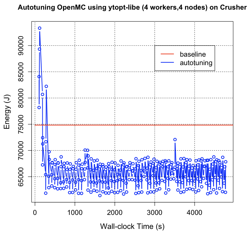
Figure 21: Autotuning OpenMC with the performance metric energy on 8 GPUs using ytopt-libe

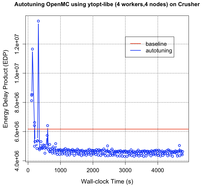
Figure 22: Autotuning OpenMC with the performance metric EDP on 8 GPUs using ytopt-libe

8 Conclusions

In this paper we presented our methodology and framework ytopt-libe to integrate ytopt and libEnsemble to take advantage of massively parallel resources to accelerate the autotuning process. Specifically, we focused on using the proposed framework to autotune the application OpenMC. OpenMC has seven tunable parameters, some of which have large ranges, and it is time-consuming to set the proper combination of these parameter values to achieve the best performance. We applied the proposed framework to autotune the MPI/OpenMP offload version of OpenMC based on a user-defined metric such as the FoM (particles/s) or runtime, energy, and EDP on the OLCF Frontier TDS system Crusher. The experimental results show that we achieve an improvement of up to 29.49% in FoM and up to 30.44% in EDP. For future work, we plan to use ytopt-libe to autotune the latest development version of OpenMC (which removes queue and queueless modes) on exascale systems such as OLCF Frontier and the Argonne Aurora system to investigate how different system architectures affect the performance and improve the I/O issues for slowly loading HDF5 data using parallel I/O strategies. The ytopt-libe package is available from our GitHub repo https://github.com/ytopt-team/ytopt-libensemble, and the autotuning scripts for OpenMC are avaliable from our GitHub repo https://github.com/ytopt-team/ytopt-libensemble/tree/main/ytopt-libe-openmc.

The submitted manuscript has been created by UChicago Argonne, LLC, Operator of Argonne National Laboratory (”Argonne”). Argonne, a U.S. Department of Energy Office of Science laboratory, is operated under Contract No. DE-AC02-06CH11357. The U.S. Government retains for itself, and others acting on its behalf, a paid-up nonexclusive, irrevocable worldwide license in said article to reproduce, prepare derivative works, distribute copies to the public, and perform publicly and display publicly, by or on behalf of the Government. The Department of Energy will provide public access to these results of federally sponsored research in accordance with the DOE Public Access Plan (http://energy.gov/downloads/doe-public-access-plan).

References

- [Wu(2023)] X. Wu, P. Balaprakash, M. Kruse, J. Koo, B. Videau, P. Hovland, V. Taylor, B. Gelts, S. Jana, and M. Hall (2023), ytopt: Autotuning scientific applications for energy efficiency at large scales, Proceedings of Cray User Group Conference 2023, Helsinki, Finland, May 7–11, 2023.
- [Wu(2022)] X. Wu, M. Kruse, P. Balaprakash, H. Finkel, P. Hovland, V. Taylor, and M. Hall (2022), Autotuning PolyBench benchmarks with LLVM Clang/Polly Loop Optimization Pragmas Using Bayesian Optimization, Concurrency and Computation: Practice and Experience, Volume 34, Issue 20, e6683, 2022.
- [ytopt(2023)] ytopt (2023), ytopt: a machine-learning-based autotuning software package. https://github.com/ytopt-team/ytopt.
- [Wu(2023a)] X. Wu, P. Paramasivam, and V. Taylor, Autotuning Apache TVM-based scientific applications using Bayesian optimization, SC23 Workshop on Artificial Intelligence and Machine Learning for Scientific Applications (AI4S’23), Nov. 13, 2023, Denver, CO
- [Crusher(2023)] Crusher (2023), Frontier TDS system, Oak Ridge National Lab. https://docs.olcf.ornl.gov/systems/crusher_quick_start_guide.html.
- [OpenMC(2022)] OpenMC (2022), https://openmc.org. https://github.com/jtramm/openmc_offloading_builder/tree/main.
- [ConfigSpace(2023)] ConfigSpace (2023). https://github.com/automl/ConfigSpace.
- [APEX(2023)] APEX (2023), APEX: Autonomic Performance Environment for eXascale. http://uo-oaciss.github.io/apex/
- [Wu(2020)] X. Wu, A. Marathe, S. Jana, O. Vysocky, J. John, A. Bartolini, L. Riha, M. Gerndt, V. Taylor, and S. Bhalachandra (2020), Toward an end-to-end auto-tuning framework in HPC PowerStack, Proceedings of Energy Efficient HPC State of Practice 2020 (EE HPC SOP 20), IEEE Computer Society, 2020.
- [Tramm(2022)] J. R. Tramm, P. K. Romano, J. Doerfert, A. L. Lund, P. C. Shriwise, A. R. Siegel, G. Ridley, and A. Pastrello (2022), Toward portable GPU acceleration of the OpenMC Monte Carlo particle transport code, PHYSOR 2022 – International Conference on Physics of Reactors, May 2022.
- [Romano(2015)] P. K. Romano, N. E. Horelik, B. R. Herman, A. G. Nelson, B. Forget, and K. Smith, OpenMC: A state-of-the-art Monte Carlo code for research and development, Annals of Nuclear Energy, Volume 82, pp. 90–97, 2015.
- [Hoogenboom(2011)] J. E. Hoogenboom, W. R. Martin, and B. Petrovic, The Monte Carlo performance benchmark test—aims, specifications, and first results, Proceedings of Int. Conf. on Mathematics and Computational Methods Applied to Nuclear Science and Engineering, Rio de Janeiro, Brazil, 2011.
- [Hudson(2023)] S. Hudson, J. Larson, J.-L. Navarro, and S. M. Wild. libEnsemble: A complete Python toolkit for dynamic ensembles of calculations. Journal of Open Source Software 8(92), p. 6031. 2023, https://doi.org/10.21105/joss.06031
- [Hudson(2021)] S. Hudson, J. Larson, J.-L. Navarro, and S. M. Wild. libEnsemble: A library to coordinate the concurrent evaluation of dynamic ensembles of calculations. IEEE Transactions on Parallel and Distributed Systems 33(4). pp. 977–-988, 2022. https://doi.org/10.1109/TPDS.2021.3082815
- [Hudson(2024)] S. Hudson, J. Larson, S. M. Wild, D. Bindel, and J.-L. Navarro. libEnsemble Users Manual. Version 1.1.0. Argonne National Laboratory, 2024. https://libensemble.readthedocs.io/en/latest/
- [Chang(2020)] T. H. Chang, J. Larson, L. T. Watson, and T. C. H. Lux. Managing computationally expensive blackbox multiobjective optimization problems with libEnsemble. Proceedings of the Spring Simulation Conference, 2020. https://doi.org/10.22360/springsim.2020.hpc.001
- [Neveu(2019)] N. Neveu, S. Hudson, J. Larson, and L. Spentzouris. Comparison of model-based and heuristic optimization algorithms applied to photoinjectors using libEnsemble. Proceedings of the 13th International Computational Accelerator Physics Conference, pp. 22-–24, 2019. https://doi.org/10.18429/JACoW-ICAP2018-SAPAF03
- [Ferran Pousa(2019)] A. Ferran Pousa, S. Jalas, M. Kirchen, A. Martinez de la Ossa, M. Thévenet, S. Hudson, J. Larson, A. Huebl, J.-L. Vay, and R. Lehe. Multitask optimization of laser-plasma accelerators using simulation codes with different fidelities. Proceedings of the 13th International Particle Accelerator Conference, 2022. https://doi.org/10.18429/JACoW-IPAC2022-WEPOST030
- [Theta(2022)] Cray XC40 Theta (2022), Argonne National Laboratory, https://www.alcf.anl.gov/theta
- [Summit(2022)] Summit (2022), Oak Ridge National Laboratory, https://www.olcf.ornl.gov/olcf-resources/compute-systems/summit/.
- [ProxyApps(2022)] ECP Proxy Applications Suite, https://proxyapps.exascaleproject.org/ecp-proxy-apps-suite/.
- [subprocess(2022)] Subprocess management, subprocess.Popen.communicate. https://docs.python.org/3/library/subprocess.html.
- [Whaley and Dongarra(1998)] R. C. Whaley and J. Dongarra, Automatically tuned linear algebra software, Proceedings of the 1998 ACM/IEEE Conference on Supercomputing (SC’98), 1998. http://dl.acm.org/citation.cfm?id=509058.509096
- [Tapus(2002)] C. Tapus, I. Chung and J. K. Hollingsworth, Active Harmony: Towards automated performance tuning, Proceedings of the 2002 ACM/IEEE Conference on Supercomputing (ICS’02), 2002. https://doi.org/10.1109/SC.2002.10062.
- [Chung and Hollingsworth(2006)] I. Chung and J. K Hollingsworth, A case study using automatic performance tuning for large-scale scientific programs, Proceedings of the 15th IEEE International Symposium on High Performance Distributed Computing (HPDC’06), 2006.
- [Gerndt and Ott(2010)] M. Gerndt and M. Ott, Automatic performance analysis with Periscope, Concurrency and Computation: Practice and Experience, Volume 22, No. 6, 2010.
- [Chen(2005)] C. Chen, J. Chame and M. Hall, Combining models and guided empirical search to optimize for multiple levels of the memory hierarchy, Proceedings of International Symposium on Code Generation and Optimization, 2005.
- [Tiwari and Hollingsworth(2011)] A. Tiwari and J. K Hollingsworth, Online adaptive code generation and tuning, Proceedings of the 2011 IEEE International Parallel & Distributed Processing Symposium (IPDPS’11), 2011.
- [Balaprakash(2013)] P. Balaprakash, R. B Gramacy and S. M Wild, Active-learning-based surrogate models for empirical performance running, Proceedings of the 2013 IEEE International Conference on Cluster Computing (CLUSTER’13), 2013.
- [Falch and Elster(2017)] T. L Falch and A. C Elster, Machine learning-based auto-tuning for enhanced performance portability of OpenCL applications, Concurrency and Computation: Practice and Experience, Volume 29, No. 8, 2017.
- [Ashouri(2019)] A. H. Ashouri, W.Killian, J. Cavazos, G. Palermo, and C. Silvano, A Survey on Compiler Autotuning Using Machine Learning, ACM Computing Surveys (CSUR), volume 51, No. 5, 2019.
- [Ogilvie(2017)] W. F. Ogilvie, P. Petoumenos, Z. Wang, and H. Leather, Minimizing the cost of iterative compilation with active learning, Proceedings. of the 2017 International Symposium on Code Generation and Optimization, 2017.
- [Tiwari(2009)] A. Tiwari, C. Chen, J. Chame, M. Hall, and J. K. Hollingsworth, A scalable auto-tuning framework for compiler optimization, Proceedings of the 23rd IEEE International Parallel and Distributed Computing Symposium (IPDPS’09), 2009.
- [Muralidharan(2014)] S. Muralidharan, M. Shantharam, M. Hall, M. Garland, and B. Catanzaro, Nitro: A framework for adaptive code variant tuning, Proceedings of the 2014 IEEE 28th International Parallel and Distributed Processing Symposium (IPDPS’14), 2014.
- [Sreenivasan(2019)] V. Sreenivasan, R. Javali, M. Hall, P. Balaprakash, T. R. W. Scogland, and B. R. de Supinski, A framework for enabling OpenMP autotuning, Proceedings of OpenMP: Conquering the Full Hardware Spectrum (IWOMP’19), 2019.
- [Katarzynski and Cytowski(2014)] J. Katarzynski and M. Cytowski, Towards autotuning of OpenMP applications on multicore architectures, http://arxiv.org/abs/1401.4063, 2014.
- [Mustafa(2011)] D. Mustafa, A. Aurangzeb, and R. Eigenmann, Performance analysis and tuning of automatically parallelized OpenMP applications, Proceedings of the 7th International Conference on OpenMP in the Petascale Era, 2011.
- [Liao(2010)] C. Liao, D. J. Quinlan, R. Vuduc, and T. Panas, Effective source-to-source outlining to support whole program empirical optimization, Languages and Compilers for Parallel Computing (LCPC 2009), LNCS 5898, 2010.
- [Wu(2020)] X. Wu, M. Kruse, P. Balaprakash, H. Finkel, P. Hovland, V. Taylor and M. Hall, Autotuning PolyBench benchmarks with LLVM Clang/Polly loop optimization pragmas using Bayesian optimization, Proceedings of SC20 Workshop on Performance Modeling, Benchmarking and Simulation of High Performance Computer Systems (PMBS’20), 2020.
- [Liu(2021)] Y. Liu, W. M. Sid-Lakhdar, O. Marques, X. Zhu, C. Meng, J. W. Demmel, X. S. Li, GPTune: Multitask learning for autotuning exascale aApplications, Proceedings of the 26th ACM SIGPLAN Symposium on Principles and Practice of Parallel Programming(PPoPP’21), pp. 234–246, 2021.
- [Roy(2021)] R. B. Roy, T. Patel, V. Gadepally, and D. Tiwari, Bliss: Auto-tuning complex applications using a pool of diverse lightweight learning models, Proceedings of the 42nd ACM SIGPLAN International Conference on Programming Language Design and Implementation (PLDI’21), pp. 1280–1295, 2021.
- [Miyazaki(2018)] T. Miyazaki, I. Sato, and N. Shimizu, Bayesian optimization of HPC systems for energy efficiency, High Performance Computing, pp. 44–62, 2018.
- [Willemsen(2021)] F. Willemsen, R. van Nieuwpoort, and B. van Werkhoven, Bayesian optimization for auto-tuning GPU kernels, Proceedings of the 2021 International Workshop on Performance Modeling, Benchmarking and Simulation of High Performance Computer Systems (PMBS’21), pp. 106–117, 2021, 10.1109/PMBS54543.2021.00017.
- [PROTEAS-TUNE(2023)] PROTEAS-TUNE(2023), ECP PROTEAS-TUNE, https://www.exascaleproject.org/research-project/proteas-tune/
- [PETSC/TAO(2023)] PETSC/TAO (2023), ECP PETSC/TAO, https://www.exascaleproject.org/research-project/petsc-tao/
- [ECP(2023)] ECP(2023), U.S. DOE Exascale Computing Project, https://www.exascaleproject.org
- [ExaSMR(2023)] ExaSMR(2023), ExaSMR, https://www.exascaleproject.org/research-project/exasmr/
- [Slurm(2022)] Slurm(2022), Slurm workload manager, https://slurm.schedmd.com