Inferentialist Resource Semantics
(Extended Abstract) 

Abstract

In systems modelling, a system typically comprises located resources relative to which processes execute. One important use of logic in informatics is in modelling such systems for the purpose of reasoning (perhaps automated) about their behaviour and properties. To this end, one requires an interpretation of logical formulae in terms of the resources and states of the system; such an interpretation is called a resource semantics of the logic. This paper shows how inferentialism — the view that meaning is given in terms of inferential behaviour — enables a versatile and expressive framework for resource semantics. Specifically, how inferentialism seamlessly incorporates the assertion-based approach of the logic of Bunched Implications, foundational in program verification (e.g., as the basis of Separation Logic), and the renowned number-of-uses reading of Linear Logic. This integration enables reasoning about shared and separated resources in intuitive and familiar ways, as well as about the composition and interfacing of system components.

1 Introduction

Within informatics, perhaps the most important systems concept is that of a distributed system [11, 43]. From the systems modelling perspective, with a little abstraction, one can think of a distributed system as comprising delimited collections of interconnected component systems  [25, 46, 9, 3, 13]. These systems ultimately comprise locations, at which are situated resources — understood broadly as those entities which may be manipulated by processes — relative to which processes execute, consuming, creating, moving, combining, and otherwise manipulating resources as they evolve, so delivering services. One principal use of logic is to represent, understand, and reason about such systems; this determines the field of logical systems modelling.

In this field, substructural logics are useful because of their resource interpretations. The study of such interpretations of logics, especially in the context of systems modelling, is resource semantics — see Section 3. Perhaps the most celebrated examples of resource semantics are the number-of uses reading (e.g., [24, 18, 1, 21]) of Linear Logic (LL) [19] and the sharing/separation reading (e.g., [27, 32, 33]) of the logic of Bunched Implications (BI) [27]. While both applicable to systems modelling, these two readings work in different ways and are related to different ways of doing the modelling.

The number-of-uses reading for LL concerns the dynamics of the system: formulae denote processes and resources themselves. Moreover, it is available only through its proof theory, and is not reflected in its truth-functional semantics (e.g., [18, 2, 12]). This approach is exemplified via the vending machine model:

Having a chocolate bar is denoted by $C$, and having one euro by $1{\small€}$. The formula $1{\small€}\to C$ (using material implication) is intended to denote ‘one euro buys one chocolate bar’, since (by modus ponens) $1€$ together $1{\small€}\to C$ yield $C$. However this probably doesn’t model the economy we meant as it also follows that $1{\small€}\to C\land C$ (i.e., ‘one euro buys two chocolate bars’)! The problem is that euro is a resource that should be consumed in a transaction, yielding only one chocolate bar. We can model things more carefully using linear implication and the tensor product: from $1{\small€}\multimap C$, we infer $1{\small€}\otimes 1{\small€}\multimap C\otimes C$ — ‘two euros buys two chocolate bars’, but not $1{\small€}\multimap C\otimes C$ — ‘one euro buys two chocolate bars’.

Meanwhile, the sharing/separation reading of BI proceeds through its (ordered-monoidal/relational) model-theoretic semantics and, rather than the process, it concerns the composition and state of the system. This is best exemplified by its essential place in program verification — see, for example, the use of Separation Logic [22, 36] to reason about correctness of pointer-based programming languages through a specific model of BI known as the stack-heap model of computer memory, where the monoidal composition is concatenation of memory cells. The details of this and its efficacy has been discussed by Pym et al. [32, 33, 14].

While both readings are useful, they are individually limited in the context of systems modelling: sharing/separation expresses the structure of distributed systems, and number-of-uses expresses the dynamics of the resources involved. Importantly, they also operate in completely different paradigms: number-of-uses proceeds from the proof theory of LL, while sharing/separation proceeds from the model theory of BI. This paper provides a unifying framework for the two resource interpretations given above: proof-theoretic semantics (P-tS).

In this paper, we provide a definition of resource semantics that incorporates both number-of-uses and sharing/separation. Having done this, we illustrate that the recent P-tS of LL and of BI recover these readings respectively. Moreover, we show that the P-tS of BI delivers both readings simultaneously. The semantic paradigm supporting P-tS is inferentialism [5] — the view that meaning (or validity) arises from inference. Therefore, as a point of departure for this work, we adopt an inferentialist view of systems modelling in which the basis for reasoning about a system and its properties should be based on inferences over the underlying specification of the system.

In model-theoretic semantics (M-tS), logical consequence is defined in terms of truth in models — understood as abstract mathematical structures. In the standard reading of Tarski [44, 45], a propositional formula $\varphi$ follows (model-theoretically) from a context $\Gamma$ iff every model of $\varGamma$ is a model of $\varphi$. Therefore, consequence is understood as the transmission of truth. From this perspective, meaning and validity are characterized in terms of truth.

Proof-theoretic semantics (P-tS) is an alternative approach to meaning and validity in which they are characterized in terms of proofs — understood as objects denoting collections of acceptable inferences from accepted premisses. This is subtle. Crucially, P-tS is not about providing a proof system for the logic, but about explicating the meaning of the connectives in terms of proof systems. Indeed, as Schroeder-Heister [40] observes, since no formal system is fixed (only notions of inference) the relationship between semantics and provability remains the same as it has always been — in particular, soundness and completeness are desirable features of formal systems. Essentially, what differs is that proof in P-tS plays the part of truth in M-tS. One particular class of P-tS is base-extension semantics (B-eS), in which the meaning of formulae is given (essentially) by an inductively defined validity judgement $\Gamma\Vdash_{\mathscr{B}}\varphi$ relative to a base of ‘atomic’ rules. This is the account used in this paper; it is explained in detail in Section 2.

We include a brief glossary for the various logics discussed in this paper. We have several subsystems of Linear Logic (LL): intuitionistic LL is abbreviated ILL, ILL without $!$ is abbreviated IMALL, IMALL without $\,\,\&\,\,,\oplus,1,\bot$ is abbreviated IMLL. The logic of Bunched Implications is abbreviated BI. Finally, Intuitionistic Propositional Logic is abbreviated IPL.

In Section 2, we explain how B-eS works for IMALL and BI. This section provides essential technical background for what follows. In Section 3, we explain the concepts and inferentialist resource semantics as delivered by B-eS. We begin with a definition of resource semantics for distributed systems and explain in some detail how IMALL and BI instantiate it, incorporating systematically both the number-of-uses reading of IMALL and the sharing/separation semantics of BI. We conclude Section 3 with an assertion of the thesis of this paper. In Section 4, we develop detailed examples of the use of inferentialist resource semantics to model and reason about examples of distributed systems. The examples we choose — the security processes in an airport and multi-factor authentication — are intended to be both familiar and evidently generic in that it should be clear how other examples would map onto them quite naturally. In Section 5, we conclude by discussing informally how our inferentialist resource semantics applies to distributed systems in general. This builds directly on the understanding illustrated by the examples in Section 4.

2 Base-extension Semantics (B-eS)

A B-eS of a logic is a characterization of its logical constants in terms of proof and provability in systems of rules over atoms, bases. The B-eS is given by an inductively defined support relation. In this paper, we follow the paradigm of Sandqvist [37, 38, 39] and Piecha et al. [29, 28, 30]; while there are other versions than presented here (cf. [20, 41]) are not directly relevant for this work.

In this section, we define the B-eS of (intuitionistic) LL (Section 2.1) and the B-eS of BI (Section 2.2) as they directly relate to resource semantics. We briefly describe it in the context of intuitionistic propositional logic (IPL) – see Sandqvist [39] — to help understand the substructural setting.

Fix a (denumerable) set of atomic propositions $\mathbb{A}$. For IPL, an atomic rule is a natural deduction rules (in the sense of Gentzen [42]) of the following form restricted to atoms, where $p_{1},\dots,p_{n},c\in\mathbb{A}$, and the $P_{i}$s are finite sets of atoms:

$$~{}~{}c~{}~{} c\lx@proof@logical@and p_{1}[P_{1}]\ldots p_{n}[P_{n}]$$  

A base $\mathscr{B}$, which is a denumerable set of such rules, determines a derivability relation $\vdash_{\!\!\mathscr{B}}$ in the expected way, but without the use of substitution for the atoms appearing the rules; that is, one has the following closure properties: $P,p\vdash_{\!\!\mathscr{B}}p$ for any $p\in\mathbb{A}$ and $P\subseteq\mathbb{A}$; if $\mathsf{A}\in\mathscr{B}$, then $P\vdash_{\!\!\mathscr{B}}c$; and if $\mathsf{R}\in\mathscr{B}$ and $P,P_{1}\vdash_{\!\!\mathscr{B}}p_{1}$,…, $P,P_{n}\vdash_{\!\!\mathscr{B}}p_{n}$, then $P\vdash_{\!\!\mathscr{B}}c$.

Derivability in a base ($\vdash_{\!\!\mathscr{B}}$) is the base case of support in a base ($\Vdash_{\mathscr{B}}$) that gives the B-eS — that is, for any $p\in\mathbb{A}$, $\Vdash_{\mathscr{B}}p\mbox{ iff }\vdash_{\!\!\mathscr{B}}p$. The inductive case is given by clauses analogous to the definition of satisfaction in M-tS. The are a couple of important features to note. First, the clauses for various connectives can be substantially different from treatments in other semantics. For example, the B-eS for IPL by Sandqvist [39] has the following clauses for disjunction ($\lor$):

$$\Vdash_{\mathscr{B}}\varphi\lor\psi\qquad\mbox{iff}\qquad\mbox{$\forall\mathscr{C}\supseteq\mathscr{B}\,\forall\and{p}\in\mathbb{A}$, if $\varphi\Vdash_{\mathscr{C}}\and{p}$ and $\psi\Vdash_{\mathscr{C}}\and{p}$, then $\Vdash_{\mathscr{C}}\and{p}$}$$

Piecha et al. [29, 28, 30] have shown that the standard meta-level ‘or’ clause — that is, $\Vdash_{\mathscr{B}}\varphi\lor\psi$ iff $\Vdash_{\mathscr{B}}\varphi$ or $\Vdash_{\mathscr{B}}\psi$ — yields incompleteness.

Second, the treatment of non-empty context is given by a base-extension,

$$\Gamma\Vdash_{\mathscr{B}}\varphi\qquad\mbox{iff}\qquad\mbox{$\forall\mathscr{X}\supseteq\mathscr{B}$, if $\Vdash_{\mathscr{X}}\Gamma$, then $\Vdash_{\mathscr{X}}\varphi$}$$

While prima facie this use of base-extension appears to be related to pre-order in the M-tS of IPL (cf. [23]), that remains to be determined.

This brief introduction suffices to highlight some important features of B-eS. The remainder will now give the detail in the context of substructural logic.

2.1 Base-extension Semantics of (intuitionistic) LL

A B-eS of a substructural logic requires a few modifications to the treatment of IPL outlined above. This is discussed in detail by the authors [17, 16]. In this section, we present the treatment of LL provided by the authors [17] (with the additives given by Buzoku [8, 7]).

Again, fix a (denumerable) set of atoms $\mathbb{A}$. We use lower-case Roman letters $c,p,\ldots$ to denote elements of $\mathbb{A}$, upper-case Roman letters $P,U,V\ldots$ to denote (finite) multisets of elements of $\mathbb{A}$, lower-case Greek letters $\varphi,\psi,\chi,\ldots$ to denote formulae, and upper-case Greek letters $\Gamma,\Delta,\ldots$ to denote (finite) multisets of formulae. More generally, for a set $X$, we write $\mathbb{M}(X)$ to denote the set of (finite) multisets of elements of $X$; we use to denote multiset union.

For ILL, atomic rules take are in the format used by Bierman [4] and Negri [26]; that is, rules have premisses with (possibly empty) multiset of hypothesises that are divided into sets,

$$~{}~{}c~{}~{}\qquad c\lx@proof@logical@and\left\{\raisebox{-9.00002pt}{$p_{1}^{(1)}\quad\ldots\quad p_{n_{1}}^{(1)}\,\,[P_{1}^{(1)}]\hskip 25.20006pt[P_{n_{1}}^{(1)}]$}\right\}\ldots\left\{\raisebox{-9.00002pt}{$p_{1}^{(k)}\quad\ldots\quad p_{n_{k}}^{(k)}\,\,[P_{1}^{(k)}]\hskip 25.20006pt[P_{n_{k}}^{(k)}]$}\right\}$$

A base $\mathscr{B}$ is a denumerable set of such rules and the derivability conditions reflect their intended reading:

• ref. $p\vdash_{\!\!\mathscr{B}}p$ for any $p\in\mathbb{A}$

• app. If $\mathsf{A}\in\mathscr{B}$, then $\varnothing\vdash_{\!\!\mathscr{B}}c$; and if $\mathsf{R}\in\mathscr{B}$ and there are $C_{1},\ldots,C_{k}\in\mathbb{M}(\mathbb{A})$ s.t. $C_{i}\!\mathrel{\fatcomma}\!P_{j}^{(i)}\vdash_{\!\!\mathscr{B}}p_{j}^{(i)}$ for every $j=1\ldots n_{i}$ and $i=1\ldots k$, then $C_{1}\!\mathrel{\fatcomma}\!\ldots\!\mathrel{\fatcomma}\!C_{k}\vdash_{\!\!\mathscr{B}}c$.

This has been made substructural in ref by restricting the assumption to be the atom itself and in app by combining assumptions for each collection of premisses.

Relative to this notion of derivability in a base, the definition of support for ILL without $!$ (i.e., IMALL) is partly given in Figure 1. The validity judgement, $\Gamma\Vdash\varphi$, is defined as $\Gamma\Vdash_{\mathscr{B}}^{\varnothing}\varphi$, for any base $\mathscr{B}$, and extends to multiset conclusions in the evident way. Support is shown to be sound and complete [17, 8, 7]: $\Gamma\vdash_{\text{ILL}}\varphi$ iff $\Gamma\Vdash\varphi$. There are a few things to note: first, support is now parametrized by a multiset of atoms, whose role is to track movement of data; second, the clauses are as anticipated by IPL, but rendered substructural relative to the new parametrization (e.g., $\&$ copies the multiset of atoms while splits it).

 

$$\begin{array}[]{l@{\quad}c@{\quad}l@{\quad}r}\mbox{$\Vdash_{\mathscr{B}}^{\and{P}}\and{p}$}&\mbox{iff}&\mbox{$\and{P}\vdash_{\!\!\mathscr{B}}\and{p}$}&\mbox{(At)}\\[1.42262pt] \mbox{$\Vdash_{\mathscr{B}}^{\and{P}}\varphi\multimap\psi$}&\mbox{iff}&\mbox{$\varphi\Vdash_{\mathscr{B}}^{\and{P}}\psi$}&\mbox{($\multimap$)}\\[1.42262pt] \mbox{$\Vdash_{\mathscr{B}}^{\and{P}}\varphi\otimes\psi$}&\mbox{iff}&\mbox{$\forall\mathscr{X}\supseteq\mathscr{B}$, $\forall\and{U}$, $\forall\and{p}$, if $\varphi\!\mathrel{\fatcomma}\!\psi\Vdash_{\mathscr{X}}^{\and{U}}\and{p}$, then $\Vdash_{\mathscr{X}}^{\and{P}\mathrel{\fatcomma}\and{U}}\and{p}$}&\mbox{($\otimes$)}\\[1.42262pt] \mbox{$\Vdash_{\mathscr{B}}^{\and{P}}\varphi\oplus\psi$}&\mbox{iff}&\mbox{$\forall\mathscr{X}\supseteq\mathscr{B},\,\forall U,\,\forall p$, if $\varphi\Vdash_{\mathscr{X}}^{U}p$ and $\psi\Vdash_{\mathscr{X}}^{U}p$, then $\Vdash_{\mathscr{X}}^{P\mathrel{\fatcomma}U}p$}&\mbox{($\oplus$)}\\[1.42262pt] \mbox{$\Vdash_{\mathscr{B}}^{\and{P}}\varphi\,\,\&\,\,\psi$}&\mbox{iff}&\mbox{$\Vdash_{\mathscr{B}}^{P}\varphi$ and $\Vdash_{\mathscr{B}}^{P}\psi$}&\mbox{($\&$)}\\[-2.27621pt] &\vdots&&\\ \mbox{$\Vdash_{\mathscr{B}}^{P}\Gamma\!\mathrel{\fatcomma}\!\Delta$}&\mbox{iff}&\mbox{$\exists\and{U},\and{V}$ s.t. $\and{P}=(\and{U}\!\mathrel{\fatcomma}\!\and{V})$, $\Vdash_{\mathscr{B}}^{\and{U}}\Gamma$, and $\Vdash_{\mathscr{B}}^{V}\Delta$}&\mbox{(\,\,$\!\mathrel{\fatcomma}\!$\,\,)}\\[1.42262pt] \mbox{$\Gamma\Vdash_{\mathscr{B}}^{P}\varphi$}&\mbox{iff}&\mbox{$\forall\mathscr{X}\supseteq\mathscr{B}$ and $\forall\and{U}$, if $\Vdash_{\mathscr{X}}^{\and{U}}\Gamma$, then $\Vdash_{\mathscr{X}}^{\;\and{P}\;\!\mathrel{\fatcomma}\!\;\and{U}}\varphi$}&\mbox{\hypertarget{imll-inf}{(Inf)}}\\[1.42262pt] \end{array}$$

 

Figure 1: Base-extension Semantics for IMALL

In Section 3, we discuss how this semantics expresses the number-of-uses reading of IMALL. Intuitively, the indexed multiset of atoms denotes available resources. The vending machine example in Section 1 is easily modelled: let $\Gamma$ be a theory defining the machine’s behaviour (e.g., $1{\small€}\multimap C$) and let $\mathscr{V}$ be any base supporting that theory (i.e., $\Vdash_{\mathscr{V}}^{\varnothing}\Gamma$), then the situation ‘one euro will buy one chocolate bar’ corresponds to the judgement $\Vdash_{\mathscr{V}}^{1{\small€}}C$.

What about the exponential, ‘$!$’  ? Intuitively, its resource reading is that the resource to which it is applied is unbounded — zero or arbitrarily many instances of it may be used. This can be expressed in the presented set-up, but requires a lot of delicate overhead, as given in [8, 7], that is not essential for presenting our basic account of resource semantics and its use in modelling distributed systems.

2.2 Base-extension Semantics of BI

Here, we recall a B-eS for BI [16] and give the technical development needed to explain and illustrate it. Its resource interpretation is discussed in Section 3.

Essentially, BI is the free combination of IPL — with connective $\top,\land,\lor,\to$ — and IMLL — with connective $\top^{\ast},\mathrel{\ast},\mathrel{-\mkern-12.0mu-\mkern-12.0mu\ast}$. Consequently, contexts in BI are not one of the standard data structures (e.g., sets, multiset, lists), but rather bunches, a term that derives from the relevance logic literature — see, for example, Read [34]. Essentially, bunches in BI are the free combination of the context constructors of IPL — denoted $\varnothing_{\!+}$ and — and IMLL — denoted $\varnothing_{\!\times}$ and .

Definition 1 (Bunch)

Let $\mathbb{X}$ be some data one wants to generate bunches over, then $\mathbb{B}(\mathbb{X})$ is defined as follows: $X::=x\in\mathbb{X}\mid\varnothing_{\!+}\mid\varnothing_{\!\times}\mid X\!\mathrel{\fatsemi}\!X\mid X\!\mathrel{\fatcomma}\!X$ .

If $\mathbb{F}$ is the set of formulas (over atoms $\mathbb{A}$) in BI, then $\mathbb{B}(\mathbb{F})$ is the set of bunches of formulas. A sequent in BI is a pair $\Gamma\triangleright\varphi$ in which $\Gamma\in\mathbb{B}(\mathbb{F})$ and $\varphi\in\mathbb{F}$.

If a bunch $\Delta$ is a sub-tree of a bunch $\Gamma$, then $\Delta$ is a sub-bunch of $\Gamma$. Importantly, sub-bunches are sensitive to occurrence — for example, in the bunch $\Delta\!\mathrel{\fatcomma}\!\Delta$, each occurrence of $\Delta$ is a different sub-bunch. We may write $\Gamma(\Delta)$ to express that $\Delta$ is a sub-bunch of $\Gamma$. This notation is traditional for BI [27], but requires careful handling. To avoid confusion, we never write $\Gamma$ and later $\Gamma(\Delta)$ to denote the same bunch, but rather maintain one presentation. The substitution of $\Delta$ for $\Delta^{\prime}$ in $\Gamma$ is denoted $\Gamma(\Delta)[\Delta\mapsto\Delta^{\prime}]$. This is not a universal substitution, but a substitution of the particular occurrence of $\Delta$ meant in writing $\Gamma(\Delta)$. The bunch $\Gamma(\Delta)[\Delta\mapsto\Delta^{\prime}]$ may be denoted $\Gamma(\Delta^{\prime})$ when no confusion arises.

Since bunches are not as standard as other data structures, we give some details about their meta-theory that is essential to understanding BI. We require the notion of a contextual bunch, which we think of a contextual bunch as a bunch with a hole — cf. nests with a hole in work by Brünnler [6]. This is already suggested by the substitution notation, but it is worth giving explicit mathematical treatment to avoid confusion.

 

$$\begin{array}[]{lc@{\quad}lr}\Vdash_{\mathscr{B}}^{\and{S}}\and{p}&\text{iff}&\and{S}\vdash_{\mathscr{B}}\and{p}&\ref{cl:BI-BeS-supp:At}\\[1.42262pt] \Vdash_{\mathscr{B}}^{\and{S}}\varphi\land\psi&\text{iff}&\mbox{$\forall\mathscr{X}\supseteq\mathscr{B},\forall\and{U}(\cdot),\forall p$, if $\varphi\!\mathrel{\fatsemi}\!\psi\Vdash_{\mathscr{X}}^{\and{U}(\cdot)}\and{p}$, then $\Vdash_{\mathscr{X}}^{\and{U(S)}}\and{p}$}&\ref{cl:BI-BeS-supp:conjunction}\\[1.42262pt] \Vdash_{\mathscr{B}}^{\and{S}}\varphi\mathrel{\ast}\psi&\text{iff}&\mbox{$\forall\mathscr{X}\supseteq\mathscr{B},\forall\and{U}(\cdot),\forall p$, if $\varphi\!\mathrel{\fatcomma}\!\psi\Vdash_{\mathscr{X}}^{\and{U}(\cdot)}\and{p}$, then $\Vdash_{\mathscr{X}}^{\and{U(S)}}\and{p}$}&\ref{cl:BI-BeS-supp:mand}\\[1.42262pt] \Vdash_{\mathscr{B}}^{\and{S}}\varphi\lor\psi&\text{iff}&\forall\mathscr{X}\supseteq\mathscr{B},\forall\and{U}(\cdot),\forall p,\text{if }\varphi\Vdash_{\mathscr{X}}^{\and{U}(\cdot)}\and{p}\text{ and }\psi\Vdash_{\mathscr{X}}^{\and{U(\cdot)}}\and{p},\text{ then }\Vdash_{\mathscr{X}}^{\and{U(S)}}\and{p}&\ref{cl:BI-BeS-supp:disjunction}\\[1.42262pt] \Vdash_{\mathscr{B}}^{\and{S}}\varphi\to\psi&\text{iff}&\varphi\Vdash_{\mathscr{B}}^{\and{S}\mathrel{\fatsemi}(\cdot)}\psi&\ref{cl:BI-BeS-supp:implication}\\[1.42262pt] \Vdash_{\mathscr{B}}^{\and{S}}\varphi\mathrel{-\mkern-12.0mu-\mkern-12.0mu\ast}\psi&\text{iff}&\varphi\Vdash_{\mathscr{B}}^{\and{S}\mathrel{\fatcomma}(\cdot)}\psi&\ref{cl:BI-BeS-supp:wand}\\[-1.99168pt] &\vdots&&\\ \Vdash_{\mathscr{B}}^{\and{S}}\Gamma\!\mathrel{\fatcomma}\!\Delta&\mbox{iff}&\mbox{$\exists\and{Q_{1}},\and{Q_{2}}\in\mathbb{B}(\mathbb{A})$ such that $\and{S}\succeq\and{Q_{1}}\!\mathrel{\fatcomma}\!\and{Q_{2}}$, $\Vdash_{\mathscr{B}}^{\and{Q_{1}}}\Gamma$, and $\Vdash_{\mathscr{B}}^{\and{Q_{2}}}\Delta$}&\ref{cl:BI-BeS-supp:mcomma}\\[1.42262pt] \Vdash_{\mathscr{B}}^{\and{S}}\Gamma\!\mathrel{\fatsemi}\!\Delta&\mbox{iff}&\mbox{$\exists\and{Q_{1}},\and{Q_{2}}\in\mathbb{B}(\mathbb{A})$ such that $\and{S}\succeq\and{Q_{1}}$, $\and{S}\succeq\and{Q_{2}}$, $\Vdash_{\mathscr{B}}^{\and{Q_{1}}}\Gamma$, and $\Vdash_{\mathscr{B}}^{\and{Q_{2}}}\Delta$}&\ref{cl:BI-BeS-supp:acomma}\\[1.42262pt] \Gamma\Vdash_{\mathscr{B}}^{\and{R(\cdot)}}\psi&\text{iff}&\forall\mathscr{X}\supseteq\mathscr{B},\forall\and{U}\in\mathbb{B}(\mathbb{A}),\text{ if }\Vdash_{\mathscr{X}}^{\and{U}}\Gamma,\text{ then }\Vdash_{\mathscr{X}}^{\and{R(U)}}\psi&\ref{cl:BI-BeS-supp:inf}\end{array}~{}\vspace{-2mm}$$

$$\scriptsize\begin{array}[]{c}\and{Q}\triangleright\and{q}\\[5.69054pt] \and{P}\triangleright\and{p}\lx@proof@logical@and\and{P}_{1}\triangleright\and{p}_{1}\ldots\and{P}_{n}\triangleright\and{p}_{n}\end{array}\quad\begin{array}[]{ll}\hypertarget{def:derivability-in-a-base:taut}{\textsc{taut}}:&\mbox{$\and{p}\vdash_{\mathscr{B}}\and{p}$}\\ \hypertarget{def:derivability-in-a-base:initial}{\textsc{initial}}:&\mbox{If $\mathsf{A}\in\mathscr{B}$, then $\and{Q}\vdash_{\mathscr{B}}\and{q}$}\\ \hypertarget{def:derivability-in-a-base:rule}{\textsc{rule}}:&\mbox{If $\mathsf{R}\in\mathscr{B}$ and $\and{P}_{1}\vdash_{\mathscr{B}}\and{p}_{1},\dots,\and{P}_{n}\vdash_{\mathscr{B}}\and{p}_{n}$, then $\and{P}\vdash_{\mathscr{B}}\and{p}$}\\ \hypertarget{def:derivability-in-a-base:weak}{\textsc{weak}}:&\mbox{If $\and{P}(\and{Q})\vdash_{\mathscr{B}}\and{p}$, then $\and{P}(\and{Q}\fatsemi\and{Q}^{\prime})\vdash_{\mathscr{B}}\and{p}$, for any $\and{Q}^{\prime}\in\mathbb{B}(\mathbb{A})$}\\ \hypertarget{def:derivability-in-a-base:cont}{\textsc{cont}}:&\mbox{If $\and{P}(\and{Q}\fatsemi\and{Q})\vdash_{\mathscr{B}}\and{p}$, then $\and{P}(\and{Q})\vdash_{\mathscr{B}}\and{p}$}\\ \hypertarget{def:derivability-in-a-base:exch}{\textsc{exch}}:&\mbox{If $\and{P}(\and{Q})\vdash_{\mathscr{B}}\and{p}$ and $\and{Q}\equiv\and{Q}^{\prime}$, then $\and{P}(\and{Q}^{\prime})\vdash_{\mathscr{B}}\and{p}$.}\\ \hypertarget{def:derivability-in-a-base:cut}{\textsc{cut}}:&\mbox{If $\and{T}\vdash_{\mathscr{B}}\and{q}$ and $\and{S}(\and{q})\vdash_{\mathscr{B}}\and{p}$, then $\and{S}(\and{T})\vdash_{\mathscr{B}}\and{p}$.}\end{array}$$

 

Figure 2: Base-extension Semantics for BI

Definition 2 (Contextual Bunch)

A contextual bunch (over $\mathbb{X}$) is a function $b:\mathbb{B}(\mathbb{X})\to\mathbb{B}(\mathbb{X})$ such that there is $\Gamma(\Delta)\in\mathbb{B}(\mathbb{X})$ and $b(\varSigma)=\Gamma(\varSigma)$ for any $\varSigma\in\mathbb{B}(\mathbb{X})$. The identity on $\mathbb{B}(\mathbb{X})$ is a contextual bunch, it is denoted $(\cdot)$. The set of all contextual bunches (over $\mathbb{X}$) is $\dot{\mathbb{B}}(\mathbb{X})$.

Observe that $\dot{\mathbb{B}}(\mathbb{X})$ can be identified as the subset of $\mathbb{B}(\mathbb{X}\cup\{\circ\})$, where $\circ\not\in\mathbb{X}$, in which bunches contain a single occurrence of $\circ$. Specifically, if $b(x)=\Gamma(x)$, then identify $b$ with $\Gamma(\circ)\in\mathbb{B}(\mathbb{X}\cup\{\circ\})$. We write $\Gamma(\cdot)$ for the contextual bunch identified with $\Gamma(\circ)$. We require a notion of equivalence on bunches.

Definition 3 (Coherent Equivalence)

Bunches $\Gamma,\Gamma^{\prime}\in\mathbb{B}(\mathbb{X})$ are coherently equivalent when $\Gamma\equiv\Gamma^{\prime}$, where $\equiv$ is the least relation satisfying: commutative monoid equations for with unit $\varnothing_{\!+}$ and for with unit $\varnothing_{\!\times}$, and coherence (i.e., if $\Delta\equiv\Delta^{\prime}$ then $\Gamma(\Delta)\equiv\Gamma(\Delta^{\prime}))$.

In practice, bunches used for data structures are regarded as the syntactic constructions in $\mathbb{B}(\mathbb{X})$ modulo coherent equivalence.

We require a way to express the structurality of the additive context-former.

Definition 4 (Bunch-extension)

The bunch-extension relation $\succeq$ is the least relation satisfying: $\Gamma\equiv\Gamma^{\prime}[\Delta\mapsto\Delta\fatsemi\Delta^{\prime}]$ implies $\Gamma\succeq\Gamma^{\prime}$, and together $\Gamma\succeq\Gamma^{\prime}$ and $\Gamma^{\prime}\succeq\Gamma^{\prime\prime}$ imply $\Gamma\succeq\Gamma^{\prime\prime}$.

This concludes the preliminaries required on bunches for the B-eS of BI. The notion of base used for BI diverges from the above as natural deduction in the sense of Gentzen [42] appears insufficiently expressive to make all the requisite distinctions with regards to multiplicative and additive structures in bunches. Accordingly, we move to a sequent calculus perspective.

The B-eS for BI is given in Figure 2 in which $S\in\mathbb{B}(\mathbb{A})$, $\and{R}(\cdot)\in\dot{\mathbb{B}}(\mathbb{A})$, $\Gamma,\Delta\in\mathbb{B}(\mathbb{F})$. The validity judgement, $\Gamma\Vdash\varphi$, is defined as $\Gamma\Vdash_{\mathscr{B}}^{(\cdot)}\varphi$, for any base $\mathscr{B}$. Validity extends to bunched conclusions in the evident way. Support is sound and complete with regard to consequence for BI, $\vdash_{\text{BI}}$, (see, e.g., [27, 31, 15, 16]):

Theorem 2.1 (Gu et al. [16])

$\Gamma\vdash_{\emph{BI}}\varphi$ iff $\Gamma\Vdash{}\varphi$.

The proof of this (and that of the corresponding result for IMLL [17]) is inspired by Sandqvist’s corresponding proof for IPL [39].

There are a few things to note about the support judgement. First, in contrast to the treatment of IPL [39] discussed in Section 1, support is now also parametrized by a bunch of atoms. In Section 3, we see that these may usefully be thought of as resources. The role of this bunch can be seen particularly clearly in the 2.2 clause in Figure 2: the resources required for the sequent $\Gamma\triangleright\varphi$ are combined with those required for $\Gamma$ in order to deliver those required for $\varphi$.

Second, the treatment of the support of a combination of contexts $\Gamma\!\mathrel{\fatcomma}\!\Delta$ follows the naïve Kripke-style interpretation of multiplicative conjunction, corresponding to an introduction rule in natural deduction, but the support of the tensor product $\varphi\otimes\psi$ follows the form of a natural deduction elimination rule. The significance of this is explored in Section 3.

3 Inferentialist Resource Semantics

We give a systematic account of how B-eS can be used to give an account of the resource semantics in which formulae are interpreted as assertions about the flow of resources in a distributed system, expressing both the sharing/separation interpretation of BI [32] and the number-of-uses reading of LL. It is also related to the syntactic resource semantics of Pfenning and Reed [35]. After the conceptual understanding in this section, we then give detailed examples in Section 4.

In the context of models of distributed systems that are formulated in terms of locations, resources, and processes, we begin with a conceptual definition of resource semantics, as follows:

A resource semantics for a system of logic is an interpretation of its formulae as assertions about states of processes and is expressed in terms of the resources that are manipulated by those processes.

This definition requires a few notes: we intend no restriction on the assertions that are to be included in the scope of this definition; we intend the manipulation of resources by the system’s processes to include consuming/using resources, creating resources, copying/deleting resources, and moving resources between locations; assertions may refer not only to ground states but also ‘higher-order’ assertions about state transitions.

Moreover, we require that an adequate resource semantics should be able to provide accounts of the following concepts: counting of resources, composition of resources, comparison of resources, sharing of resources, and separation of resources. We illustrate all of these concepts through examples in Section 4.

In the B-eS we have presented, it is the (Inf) clause that articulates the consequence relation free of the structure of the connectives. Indeed, whilst the semantic clauses for connectives vary in the B-eS for LL and BI, their (Inf) clauses follow a similar rationale. This is no coincidence: $\Gamma\Vdash\varphi$ is about the transmission of validity, thus its definition reflects the semantic paradigm rather than of the specific logic system. Indeed, analogously in M-tS, $\Gamma\Vdash\varphi$ expresses that ‘for any model $\mathfrak{M}$, if $\Gamma$ is true in $\mathfrak{M}$, then so is $\varphi$’, regardless of the specific logic and semantics of interest. The power of B-eS to unify the aforementioned resource interpretations can be summarized in the following general pattern of support judgement and its semantics clauses for IMLL LL and BI — (Inf) is the key clause that connects the left- and right-sides of the support judgement, free of reference to connectives:

$${\small\Gamma\Vdash_{\mathscr{B}}^{S(\cdot)}\varphi\quad\text{iff}\quad\forall\mathscr{C}\supseteq\mathscr{B},\forall U\in\mathbb{R}(\mathbb{A}),\text{ if }\Vdash_{\mathscr{C}}^{U}\Gamma,\text{ then }\Vdash_{\mathscr{C}}^{S(U)}\varphi}$$ (Gen-Inf)

Let us spell out each ingredient of (Gen-Inf) and their roles in the resource semantics, which describes the execution of certain policy in a system:

• $\varphi$ is a formula of the chosen logic. It is an assertion describing (a possible state of) the system

• $\Gamma$ is collection (e.g., multiset, bunch, etc) of formulas. It specifies a policy describing the executions of a system’s processes

• $\mathbb{R}(\mathbb{A})$ is some choice of atomic resource (e.g., multisets of atoms in ILL, bunches of atoms in BI)

• $S(\cdot)$ is some contextual atomic resource, such that whenever combined with some atomic resource in $\mathbb{R}(\mathbb{A})$, it returns a ‘richer’ atomic resource (e.g., multisets of atoms in IMLL, contextual bunches in BI). It specifies the resources that are available for the system model’s processes to execute according to the given policy

• $\mathscr{B},\mathscr{C}$ are bases of one’s choice. They are models, and $\Vdash_{\mathscr{C}}^{U}\Gamma$ reads as $\mathscr{C}$ is a model of policy $\Gamma$ when supplied with resource $U$.

Putting these all together, the support judgement $\Gamma\Vdash_{\mathscr{B}}^{S(\cdot)}\varphi$ says that, if policy $\Gamma$ were to be executed with contextual resource $S(\cdot)$ based on the model $\mathscr{B}$, then the result state would satisfy $\varphi$. (Gen-Inf) explains how such execution is triggered: for arbitrary model $\mathscr{C}$ that extends $\mathscr{B}$, if policy $\Gamma$ is met in model $\mathscr{C}$ using some resource $U$, then $\Gamma$ could be executed, and the resulting state — which consumes $U$ in the available contextual resource $S(\cdot)$ — satisfies $\varphi$.

We demonstrate how this general resource interpretation retrieves the number-of-uses reading and the sharing/separation semantics when instantiated in ILL (in particular, IMALL) and BI, respectively.

Linear Logic.

Following Section 2.1, we restrict ourselves to IMALL. In this context, a multiset of atoms $P$ denotes a contextual resource $S(\cdot)$ through multiset union — that is, $S(\cdot):U\mapsto P\!\mathrel{\fatcomma}\!U$.

The number-of-uses interpretation of LL instantiates the definition of resource semantics above as follows: a formula $\varphi$ asserts that the system has some resources ‘$\varphi$’ (discussed below) and an implication $\varphi\multimap\psi$ asserts that the system has a process that uses the resources ‘$\varphi$’ and yields resources ‘$\psi$’. What resources are ‘$\varphi$’ and ‘$\psi$’? That depends on the policy $\mathscr{B}$ governing the system; for example, when the policy is empty ($\mathscr{B}=\varnothing$) and $\varphi$ and $\psi$ are atoms $p$ and $q$, respectively, then ‘$\varphi$’ is $p$ and ‘$\psi$’ is $q$ — we give further examples below. Understanding that this interpretation is relativized to a policy is essential; for example, when $\mathscr{B}$ contains an axiom $\mathsf{A}$, then one has an indefinite amount of the resource $c$ available.

The clauses in Figure 1 enable this way of reading number-of-uses as a resource semantics; that is, they explicate inductively how a formula is interpreted as a collection of resources relative to a policy — from $\Vdash_{\mathscr{B}}^{P}\varphi\multimap\psi$, one recovers a judgement $\Vdash_{\mathscr{B}\cup\mathscr{C}}^{P\mathrel{\fatcomma}U}\psi$, in which $U$ is ‘$\varphi$’ as determined by $\mathscr{C}$. We illustrate for some of connectives to show how their number-of-uses reading manifest:

• $\&$: This clause very clearly says that $\varphi\,\,\&\,\,\psi$ denotes that $\varphi$ and $\psi$ are available processes that each require the same resources; in other words, both process $\varphi$ and $\psi$ may be done, but only one will be done

•  : Similar to the above, both process $\varphi$ and $\psi$ may be done, but this time both must be done, so the resources must be divided in some suitable way

• $\otimes$: One may expect this clause to take precisely the same form as (  ), but taking the elimination form instead ensures a certain coherence in the system [17]. Indeed, taking this form, the clause allows us to see precisely how a formula denotes a collection of resources relative to a policy.

  Let us return to $\varphi\multimap\psi$. We already considered the case in which both $\varphi$ and $\psi$ are atoms. Suppose now that $\varphi$ is a tensor of atoms (i.e., $\varphi:=p_{1}\otimes\ldots\otimes p_{n}$). Again, choosing the simplest possible $\mathscr{B}$ to model this process and make ‘$\varphi$’ as plain as possible, the judgement $\Vdash{}\varphi\multimap\psi$ can be reduced to $p_{1}\!\mathrel{\fatcomma}\!\ldots\!\mathrel{\fatcomma}\!p_{n}\vdash_{\!\!\mathscr{B}}q$, in which $\mathscr{B}$ is simply a policy for a process that uses resources $\varphi$ and yields the resources $\psi$

  In general, one has $\text{`$\varphi$'}\vdash_{\!\!\mathscr{B}\cup\mathscr{C}}q$, in which $\mathscr{C}$ ensures that ‘$\varphi$’ behaves as a tensor of $p_{1},\ldots,p_{n}$ — for example, ‘$\varphi$’ can be a single atom and $\mathscr{C}$ may simulate the appropriate introduction and elimination rules,

  $$\text{`$\varphi$'}\lx@proof@logical@and\{p_{1}\}\ldots\{p_{n}\}\qquad x\lx@proof@logical@and\raisebox{-9.00002pt}{$\{\text{`$\varphi$'}\}$}\left\{\begin{array}[]{c}[p_{1}\!\mathrel{\fatcomma}\!\ldots\!\mathrel{\fatcomma}\!p_{n}]\\ x\end{array}\right\}$$

  A similar analysis can be made for when $\psi$ is a tensor-formula

• $\oplus$: This connective denotes non-deterministic choice: one of $\varphi$ or $\psi$ will fire, but we do not know which. The elimination rule format of the clause expresses precisely this: what the process $\varphi$ and $\psi$ can both yields with resources $U$, is yielded by $\varphi\oplus\psi$ with resources $U$.

This suffices to illustrate how the number-of-uses reading of LL manifests in its B-eS; the remaining connectives follow similarly. In the treatment of $\otimes$, we have concentrated on it as a pre-/post- condition of $\multimap$ (as opposed to the combination of two process that both execute as in ). This is to explicate how the format of the clause, which indeed passes through , supports the interpretation of formulae as assertions about resources.

Bunched Implications.

Briefly, a distributed system is comprised of components that exchange and process resources (see Section 5 for more on this). Two components share resources when they use the available resource at the same time and separate resources when the available resources must be divided between components. The sharing/separation interpretation of BI (see Pym [32]) pertains to modelling this aspect of the architecture of distributed systems. We illustrate how this manifests in the B-eS of BI relative to the notation in (Gen-Inf).

First, the bunch of atoms $U$ denotes the available resources. If $V$ and $W$ are collections of resources, then $V\mathrel{\fatsemi}W$ denotes a collection of resources such that each sub-collection may be shared — that is, components that share resources may use both $V$ and $W$ simultaneously, just $V$, just $W$, or one component uses $V$ while the other uses $W$ — and $V\!\mathrel{\fatcomma}\!W$ denotes a collection of resource such that each sub-collection must be used separately. This follows from the - and -clauses, observing also role played by bunch-extension in those clauses.

Second, the bunch $\Gamma$ describes the architecture of the system. The two context-formers provide the sharing/separation reading: if $\Gamma$ and $\Delta$ describe system policies for two components, then $\Gamma\!\mathrel{\fatsemi}\!\Delta$ describes a system policy in which those components share resources, and $\Gamma\!\mathrel{\fatcomma}\!\Delta$ describes a system policy in which they separate resources. Again, this is immediately expressed by the - and -clauses as the available resources are copied or divided between the sub-bunches, respectively. Intuitive readings of the associated units follow similarly.

Third, $\varphi$ is an assertion about the state of the system in terms of its sharing/separation architecture; in particular, considering some of the connectives,

• $\mathrel{\ast}$: denotes the combined effect of two separating components of the system taken as a single component

• $\land$: denotes the combined effect of two sharing components of the system taken as a single component

• $\mathrel{-\mkern-12.0mu-\mkern-12.0mu\ast}$: denotes that, if the state of the system satisfies the antecent assertion of the antecedent, then the system can be modified to satisfy the consequent assertion

• $\to$: denotes that, if the state of the system satisfies the antecedent, then the (unmodified) system also satisfies the consequent.

Presented individually in this way, the significance of these readings is, perhaps, obscured. In the base case, an atom $p$ may be thought of as the assertion that the system has a certain resource; thus, a formula $p\mathrel{-\mkern-12.0mu-\mkern-12.0mu\ast}(q_{1}\mathrel{\ast}q_{2})$ asserts that the system can move from a state in which a component may use a resource $p$ to a state in which two separate components may use $q_{1}$ and $q_{2}$. This is made more concrete in Section 4 with examples given in which these readings are instantiated in the setting of a relatable distributed systems.

Observe that restricting to the multiplicative fragment of BI one also recovers IMLL, hence one has the number-of-uses interpretation described for LL above. However, this reading actually extends to the whole of BI. The sharing/separation reading arises from the interpretation of the meta-connectives (i.e., the context-formers and their units), but one can consistently keep a number-of-uses interpretation of formulae as the way in which they make assertions about the system (i.e., they express how resources behave within the system).

The implications assert that there is a process that transitions the system from a state satisfying the antecedent to one satisfying the consequent; they are distinguished by whether or not the processes modify the system when executed. What do we mean by ‘modify’? In the basic case, we simply mean the consuming of resources; for example, both $p\mathrel{-\mkern-12.0mu-\mkern-12.0mu\ast}q$ and $p\to q$ refers to a process in which a system moves from a state in which it has a resource $p$ to one in which it has a $q$, but the former does it while consuming $p$ (in the sense of the number-of-uses reading) and the the latter only requires that $p$ is available. In the general case, we must account for the fact that the precondition of the process may itself be a process; for example, $(\varphi\mathrel{-\mkern-12.0mu-\mkern-12.0mu\ast}\psi)\mathrel{-\mkern-12.0mu-\mkern-12.0mu\ast}\chi$ denotes a process that modifies the system from the state $\varphi\mathrel{-\mkern-12.0mu-\mkern-12.0mu\ast}\psi$ (i.e., ‘there is a process …’) to the state $\chi$.

Note, since $\mathrel{-\mkern-12.0mu-\mkern-12.0mu\ast}$ modifies the system, its required resources must be private (not shared with other processes) so it uses separated resources. Since $\to$ does not modify the system its required resources are the kind that may be shared.

Thus we have described how a general view of B-eS can be instantiated to explicate the resource semantics both of logics that exhibit the sharing/separation semantics of propositions and logics that support the number-of-uses readings of propositions. We conclude this section by asserting the thesis of this paper:

The paradigm of base-extension semantics provides a framework for expressing resource interpretations of logics that uniformly admits both sharing/separation semantics — as found in logics based on bunching, such as BI and relevance logics — and number-of-uses readings — as found in the family of linear logics.

We now illustrate this thesis, in Section 4, with two familiar yet evidently generic examples of distributed systems and, in Section 5, we describe the realization of the thesis for distributed systems more generally.

4 Generic Examples: Airport Security and MFA

Having developed (a sketch of) an inferentialist resource semantics, we now illustrate the ideas by exploring some substantial examples. These examples are intended to be familiar and relatable settings in which policies are applied to located resources (e.g., [10, 9, 3]). Despite being specific in their details, they are both structurally and conceptually quite generic. Since the resource semantics of BI provided by the B-eS expresses both sharing/separation and number-of-uses approach to systems modelling, we concentrate on this logic.

Airport Security Processes.

The architecture of airport security is given in Figure 3. There are six locations — $l_{1}$, …, $l_{6}$ — each of which has an associated policy, modelled by a base ($\mathscr{B}_{i}$ at $l_{i}$). There are lots of natural notions of resource in this setting (e.g., machines, baggage, passengers, etc), but to keep things simple and focused on security, we shall restrict attention to documentation (i.e., passports, tickets, bar-codes, and so on).

   

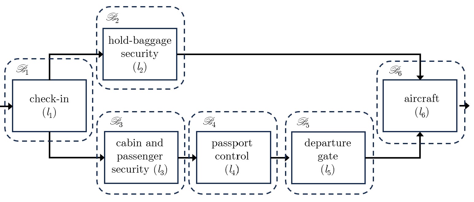
Figure 3: The Airport Security Architecture

You arrive at check-in ($l_{1}$). You show your passport, receive your boarding-card, and drop your hold-baggage. This situation is modelled by $\Gamma_{1}:=p\mathrel{-\mkern-12.0mu-\mkern-12.0mu\ast}((p\land t)\mathrel{\ast}h)$ — atom $p$ denotes your passport, $t$ denotes the boarding-card (ticket), and $h$ denotes the baggage-label. The $\mathrel{\ast}$ is used because the system bifurcates at this point and the resources $p\land t$ and $h$ go to separating components, and the $\mathrel{-\mkern-12.0mu-\mkern-12.0mu\ast}$ is used because the system is modified: the state of passport $p$ is changed as it only goes down one branch (the same as your ticket, $t$) and is no longer globally available. We discuss the use of $\mathrel{\ast}$ at $l_{1}$ in more detail below.

Next, two processes occur in parallel, one through $l_{2}$ and one through $l_{3},l_{4},l_{5}$. They are modelled by $\Delta_{1}$ and $\Delta_{2}$, respectively. Since they occur separately — that is, without sharing resources, this portion of the model is represented by the bunch $\Gamma_{2}:=\Delta_{1}\!\mathrel{\fatcomma}\!\Delta_{2}$. Indeed, the at $l_{2}$ matches the $\mathrel{\ast}$ used in $l_{1}$ above.

The top path of Figure 3 passes through hold-baggage security ($l_{2}$). Here, the label $h$ on your baggage is verified (and the baggage itself is checked). That $h$ successfully yields a validates $s_{\text{hold}}$ is denoted by $\Delta_{1}:=h\mathrel{-\mkern-12.0mu-\mkern-12.0mu\ast}s_{\text{hold}}$.

The bottom path of Figure 3 passes through $l_{3}$, $l_{4}$, and $l_{5}$, modelled by $\chi_{1}$, $\chi_{2}$, and $\chi_{3}$, respectively. This branch does not consume resources, so each is modelled using $\to$ (as opposed to $\mathrel{-\mkern-12.0mu-\mkern-12.0mu\ast}$). They share resources (e.g., passport), so $\Delta_{2}:=\chi_{1}\fatsemi\chi_{2}\fatsemi\chi_{3}$. Their ordering is enforced by the security tokens (see below), otherwise $\to$ may be used in place of  . We consider each location separately.

• You arrive at security ($l_{3}$). You must present a valid ticket to pass through the security gates. We denote this situation $\chi_{1}:=t\to s_{\text{cab}}$.

• You enter passport control ($l_{4}$). Your passport is validated and you are granted access to the gates. We denote this situation $\chi_{2}:=(s_{\text{cab}}\land p)\to s_{\text{pass}}$.

• You arrive at the gate ($l_{5}$). Your passport and ticket are checked and you are granted access. We denote this situation $\chi_{3}:=(s_{\text{pass}}\land p\land t)\to s_{\text{gate}}$.

The two separate process (i.e., $l_{2}$ and $l_{3}$ to $l_{5}$) come together at the aircraft ($l_{6}$). Here the ground-crew and the air-crew have check-lists that need to be processed and combined, but that is all hidden from you. From your perspective, both you and your hold-baggage must have been authorized to board and then, assuming clearance, the plane takes off ($f$ — flight). We model this situation by $\Gamma_{3}:=(s_{\text{gate}}\mathrel{\ast}s_{\text{hold}})\mathrel{-\mkern-12.0mu-\mkern-12.0mu\ast}f$.

We have modelled airport security in three parts, producing $\Gamma_{1}$, $\Gamma_{2}$, and $\Gamma_{3}$. How should they be composed into a single theory describing the whole system at once? Observe that overall Figure 3 describes a single process in which a passport $p$ yields flight $f$. Hence, it is modelled by an implication. The details of the process are what are described by $\Gamma_{1}$, $\Gamma_{2}$ ($\Delta_{1}$ and $\Delta_{2}$), and $\Gamma_{3}$, so we take their formula translations $\varphi_{1}$, $\varphi_{2}$ ($\psi_{1}$ and $\psi_{2}$), and $\varphi_{3}$, respectively (i.e., replace with $\land$, and with $\mathrel{\ast}$); that is,

$${\scriptsize\Gamma:=\varphi_{1}\mathrel{-\mkern-12.0mu-\mkern-12.0mu\ast}((\psi_{1}\mathrel{\ast}\psi_{2})\mathrel{-\mkern-12.0mu-\mkern-12.0mu\ast}\varphi_{3})}$$

The $\mathrel{-\mkern-12.0mu-\mkern-12.0mu\ast}$ (rather than $\to$) is appropriate because the system only flows one way; for example, having passed $l_{1}$, one cannot return to it later, the system has changed. What process do the implications explicit above represent? They are the interfacing between the various sections of system; this is part of the system and are modelled by $\mathscr{C}_{1}$ and $\mathscr{C}_{2}$, respectively.

What policy $\mathscr{B}$ models the system described by $\Gamma$? The compositional approach by which we described the model is entirely suitable, $\mathscr{B}:=\mathscr{B}_{1}\cup\ldots\cup\mathscr{B}_{6}\cup\mathscr{C}_{1}\cup\mathscr{C}_{2}$ suffices. This describes how the overall system is modelled, but it is instructive to look at bases in more detail to see how modelling of the components in this compositional approach is done.

We require $\mathscr{B}_{1}$ to support the formula $p\mathrel{-\mkern-12.0mu-\mkern-12.0mu\ast}(h\mathrel{\ast}(t\land p))$; that is, we require $\Vdash_{\mathscr{B}_{1}}^{\varnothing_{\!\times}}p\mathrel{-\mkern-12.0mu-\mkern-12.0mu\ast}((p\land t)\mathrel{\ast}h)$ to hold. Recall the clause for $\mathrel{\ast}$,

$${\small\Vdash_{\mathscr{B}_{1}}^{p}(p\land t)\mathrel{\ast}h\quad\mbox{iff}\quad\mbox{$\forall\mathscr{X}\supseteq\mathscr{B}_{1}\,\forall x\in\mathbb{A}$, if $(p\mathrel{\fatsemi}t)\!\mathrel{\fatcomma}\!h\Vdash_{\mathscr{X}}^{U(\cdot)}x$, then $\Vdash_{\mathscr{X}}^{U(p)}x$}}$$

This means that in any situation in which one can use the collection of resources $h\!\mathrel{\fatcomma}\!(t\mathrel{\fatsemi}p)$, it suffices to use the resource $p$. So, in the simplest case, it suffices for the base $\mathscr{B}_{1}$ to contain the following rules: for any $U(\cdot)\in\dot{\mathbb{B}}(\mathbb{A})$ and $x\in\mathbb{A}$,

$${\footnotesize U(p)\triangleright xU(h\!\mathrel{\fatcomma}\!t)\triangleright x}$$

This is the coarsest possible approach. In practice, check-in is a whole system unto itself (see the discussion on substitution in Section 5) and there are many internal processes that run. For example, check-in may proceed as follows: the system extracts from the passport three different parts, the name $p_{\text{name}}$, the date of birth $p_{\text{dob}}$, and the passport-number $p_{\text{num}}$; uses the passport number to issue the ticket; and uses the name on the passport and ticket together to issue the hold-baggage label. In this case, $\mathscr{B}_{1}$ may have the following rules:

$${\small p\triangleright p_{\text{name}}\qquad p\triangleright p_{\text{dob}}\qquad p\triangleright p_{\text{num}}\qquad U(p)\triangleright x\lx@proof@logical@and p_{\text{num}}\triangleright tp_{\text{name}}\!\mathrel{\fatcomma}\!t\triangleright hU(h\!\mathrel{\fatcomma}\!t)\triangleright x\qquad\raisebox{9.00002pt}{$\ldots$}}$$

where $\ldots$ denotes the part of the base that models the way in which the passport number $(p_{\text{num}})$ is used to issue the ticket $(t)$ and the name and ticket together $(p_{\text{name}}\!\mathrel{\fatcomma}\!t)$ are used to issue the hold-baggage label $(h)$. The same kind of flexibility in the modelling occurs at each location.

Multi-factor Authentication (MFA).

To illustrate how generic the notion of system used really is, we give an immediate translation to the setting of information security. The goal of MFA is to increase the overall security of systems by requiring multiple forms of verification before granting access; for example, login systems on a banking app. Such verification forms are called authentication factors, and typical examples include, inter alia, knowledge factors (e.g., passwords, pin codes, etc.), possession factors (e.g., verification code via text message or email), inherent factors (e.g., biometrics — fingerprints, voice/face recognition, etc). We model a simple MFA example of user-login for an account at a fictional bank called Bunched Money, which abstracts banking apps generally.

To access their Bunched Money account, a user needs two out of three possible authentication factors: a password $p$, a one-time passcode $o$, or a hardware fob $f$. Access is denoted by a security token $s_{\text{acc}}$. This policy can be expressed by a theory $\Gamma$ that consists of exactly one formula:

$$\Gamma:=((p\mathrel{\ast}o)\lor(p\mathrel{\ast}f)\lor(o\mathrel{\ast}f))\mathrel{-\mkern-12.0mu-\mkern-12.0mu\ast}s_{\text{acc}}$$

The $\mathrel{\ast}$ (as opposed to $\land$) because it is crucial that the two authentication factors (e.g., $p$ and $o$) are from separate sources. The separation is essential as otherwise these two factors would not enhance the security compared to a single factor — for example, two passwords are not substantially stronger than one.

Let $\mathscr{B}$ be a model of the policy describe by $\Gamma$ — that is, $\mathscr{B}$ is defined by the property $\Vdash_{\mathscr{B}}^{\varnothing_{\!\times}}\Gamma$. Let $R$ be an appropriate collection of verification factors — for example, $R:=p\!\mathrel{\fatcomma}\!o$. That access is granted under these conditions is expressed by $\Vdash_{\mathscr{B}}^{R}s_{\text{acc}}$, which indeed obtains.

5 Discussion: The Generality of the Approach

In Section 1, we discussed an abstract view of (distributed) systems based in the concepts of location, resource, and process: processes manipulate resources that reside at locations. A system is located within an environment, itself a system. The resource semantics of Section 3 has two useful features for modelling distributed systems: compositionality and substitution.

A distributed system $D$, then, comprises distinct components (or subsystems) $C_{1},\ldots,C_{n}$, each of which has its own policy, which may interface with each other. Using B-eS as described, one can model each component’s policy $\varphi_{i}$ individually by a base $\mathscr{B}_{i}$, and construct a model $\mathscr{D}$ of the overall policy for $D$ by taking the union of those bases together with some rules $\mathscr{C}$ governing their interfacing, $\mathscr{D}:=\mathscr{B}_{1}\cup\ldots\cup\mathscr{B}_{n}\cup\mathscr{C}$. In this sense, the resource semantics given by B-eS is compositional. Moreover, bases that model policies can be given at various degrees of refinement. In modelling distributed systems, this corresponds to the fact that each component $C_{i}$ of $D$ may, if useful, be thought of as a distributed system in itself; that is, one substitutes $C_{i}$ for a more detailed set of systems $C_{1}^{(i)}$,…,$C_{k}^{(i)}$, which interface to yield the overall effect of $C_{i}$. The base modelling the policy of $C_{1}^{(i)}$,…,$C_{k}^{(i)}$ still models of policy of $C_{i}$. No change is needed.

   

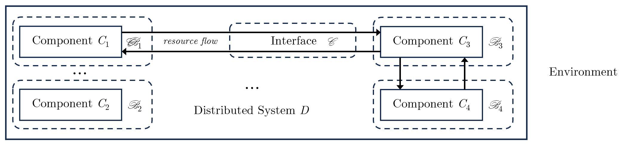
Figure 4: General Distributed System Architecture

The general picture is sketched in Figure 4. Just as in the airport example, depicted in Figure 3, the system’s processes manipulate its located resources. For example, resources may flow between component subsystems. We suggest, within Figure 4, two possible situations in describing the resource flow in compliance with the policy, with different modelling motivations.

First, we indicate, in Figure 4, that resources may, subject to compliance with policy, flow between Components $C_{1}$ and $C_{3}$. For example, a passenger may move from ground-side to air-side provided they are compliant with the airport’s security policy and here we model the component — the interface — that determines compliance with policy. In the model in Figure 3, the component $l_{3}$ can be seen as such an interface between (models of) ground-side and air-side, consisting of policies that determine whether the passenger after check-in (i.e., component $l_{1}$) could continue to passport control (i.e., component $l_{4}$).

Second, we capture only compliance with policy and do not model the details of checking it. This is the situation described in Figure 4 as the resource flow between $C_{3}$ and $C_{4}$, where we do not model the interface. In the airport example, in Figure 3, the departure gate implements a check of boarding cards and passports, and perhaps also compliance with cabin-baggage policy, but the details of these are not specified as an interface component of the model.

In general, the permitted manipulations of resources are determined by the system’s policies and these policies can be described as logical formulae that are interpreted according to the principles of the resource semantics that we have described in general in Section 3 and illustrated by example in Section 4.

Further work is to develop tools for this general set-up more formally.

Acknowledgements. This work has been partially supported by the UK EPSRC grants EP/S013008/1 and EP/R006865/1. We are grateful to Gabriele Brancati, Tim Button, Yll Buzoku, Tristan Caulfield, Diana Costa, Timo Eckhardt, Didier Galmiche, Timo Lang, Sonia Marin, Peter O’Hearn, Elaine Pimentel, Eike Ritter, Edmund Robinson, and Will Venters for discussions of various aspects of this work.

References

- [1] Abramsky, S.: Computational interpretations of linear logic. Theoretical Computer Science 111(1-2), 3–57 (1993)
- [2] Allwein, G., Dunn, J.M.: Kripke Models for Linear Logic. The Journal of Symbolic Logic 58(2), 514–545 (1993)
- [3] Anderson, G., Pym, D.: A calculus and logic of bunched resources and processes. Theoretical Computer Science 614, 63–96 (2016)
- [4] Bierman, G.M.: On Intuitionistic Linear Logic. Ph.D. thesis, University of Cambridge (1994), available as Computer Laboratory Technical Report 346
- [5] Brandom, R.: Articulating Reasons: An Introduction to Inferentialism. Harvard University Press (2000)
- [6] Brünnler, K.: Deep Sequent Systems for Modal Logic. Archive for Mathematical Logic 48(6), 551–577 (Jul 2009). https://doi.org/10.1007/s00153-009-0137-3
- [7] Buzoku, Y.: Presentation at ‘Proof-theoretic Semantics and Truth’, University of Bristol, December 2023. https://sites.google.com/view/pts-and-truth/home
- [8] Buzoku, Y.: A Proof-theoretic Semantics for Intuitionistic Linear Logic (2024), https://arxiv.org/abs/2402.01982
- [9] Caulfield, T., Pym, D.: Modelling and simulating systems security policy. In: Proceedings of the 8th International Conference on Simulation Tools and Techniques. p. 9–18. SIMUTools ’15, ICST (2015). https://doi.org/10.4108/eai.24-8-2015.2260765
- [10] Collinson, M., Monahan, B., Pym, D.: A Discipline of Mathematical Systems Modelling. College Publications (2012)
- [11] Coulouris, G., Dollimore, J., Kindberg, T., Blair, G.: Distributed Systems: Concepts and Design. Addison-Wesley Publishing Company, USA, 5th edn. (2011)
- [12] Coumans, D., Gehrke, M., van Rooijen, L.: Relational semantics for full linear logic. Journal of Applied Logic 12(1), 50–66 (2014). https://doi.org/10.1016/j.jal.2013.07.005
- [13] Galmiche, D., Lang, T., Pym, D.: Minimalistic system modelling: Behaviours, interfaces, and local reasoning, http://arxiv.org/abs/2401.16109
- [14] Galmiche, D., Kimmel, P., Pym, D.J.: A substructural epistemic resource logic: Theory and modelling applications. J. Log. Comput. 29, 1251–1287 (2019), https://api.semanticscholar.org/CorpusID:202577454
- [15] Galmiche, D., Méry, D., Pym, D.: The Semantics of BI and Resource Tableaux. Mathematical Structures in Computer Science 15(6), 1033–1088 (Dec 2005). https://doi.org/10.1017/S0960129505004858, https://doi.org/10.1017/S0960129505004858
- [16] Gheorghiu, A., Gu, T., Pym, D.: Proof-theoretic-semantics for the Logic of Bunched Implications. https://arxiv.org/abs/2311.16719 (2024), Submitted
- [17] Gheorghiu, A.V., Gu, T., Pym, D.J.: Proof-theoretic semantics for intuitionistic multiplicative linear logic. In: Ramanayake, R., Urban, J. (eds.) Automated Reasoning with Analytic Tableaux and Related Methods — TABLEAUX. pp. 367–385. Springer (2023)
- [18] Girard, J.Y.: Linear logic: its syntax and semantics. In: Advances in Linear Logic, p. 1–42. London Mathematical Society Lecture Note Series, Cambridge University Press (1995)
- [19] Girard, J.Y.: Linear logic. Theoretical computer science 50(1), 1–101 (1987)
- [20] Goldfarb, W.: On Dummett’s “Proof-theoretic Justifications of Logical Laws”. In: Piecha, T., Schroeder-Heister, P. (eds.) Advances in Proof-theoretic Semantics, pp. 195–210. Springer (2016)
- [21] Hoare, C.A.R.: Communicating Sequential Processes. Prentice-Hall International (1985)
- [22] Ishtiaq, S.S., O’Hearn, P.W.: BI as an Assertion Language for Mutable Data Structures. In: Hankin, C., Schmidt, D. (eds.) Symposium on Principles of Programming Languages — POPL, pp. 14–26. Association for Computing Machinery (ACM) (2001). https://doi.org/10.1145/360204.375719
- [23] Kripke, S.A.: Semantical Analysis of Intuitionistic Logic I. Studies in Logic and the Foundations of Mathematics 40, 92–130 (1965)
- [24] Lafont, Y.: Introduction to linear logic (1993), lecture notes from TEMPUS Summer School on Algebraic and Categorical Methods in Computer Science, Brno, Czech Republic
- [25] Milner, R.: Bigraphs as a model for mobile interaction. In: ICGT 2002, LNCS 2505. pp. 8–13. Springer Verlag (2002)
- [26] Negri, S.: A normalizing system of natural deduction for intuitionistic linear logic. Archive for Mathematical Logic 41(8), 789–810 (2002). https://doi.org/10.1007/s001530100136
- [27] O’Hearn, P.W., Pym, D.J.: The Logic of Bunched Implications. Bulletin of Symbolic Logic 5(2), 215–244 (1999). https://doi.org/10.2307/421090
- [28] Piecha, T.: Completeness in Proof-theoretic Semantics. In: Piecha, T., Schroeder-Heister, P. (eds.) Advances in Proof-theoretic Semantics, pp. 231–251. Springer (2016)
- [29] Piecha, T., de Campos Sanz, W., Schroeder-Heister, P.: Failure of Completeness in Proof-theoretic Semantics. Journal of Philosophical Logic 44(3), 321–335 (2015). https://doi.org/10.1007/s10992-014-9322-x
- [30] Piecha, T., Schroeder-Heister, P.: Incompleteness of Intuitionistic Propositional Logic with Respect to Proof-theoretic Semantics. Studia Logica 107(1), 233–246 (2019). https://doi.org/10.1007/s11225-018-9823-7
- [31] Pym, D.J.: The Semantics and Proof Theory of the Logic of Bunched Implications, Applied Logic Series, vol. 26. Springer (01 2002). https://doi.org/10.1007/978-94-017-0091-7
- [32] Pym, D.J.: Resource Semantics: Logic as a Modelling Technology. ACM SIGLOG News 6(2), 5–41 (2019). https://doi.org/10.1145/3326938.3326940
- [33] Pym, D.J., Spring, J.M., O’Hearn, P.: Why Separation Logic Works. Philosophy & Technology 32, 483–516 (2019). https://doi.org/10.1007/s13347-018-0312-8
- [34] Read, S.: Relevant Logic. Basil Blackwell (1988). https://doi.org/10.2307/2219818
- [35] Reed, J.: A Hybrid Logical Framework. Ph.D. thesis, Carnegie Mellon University (2009), available as CMU-CS-09-155
- [36] Reynolds, J.C.: Separation Logic: A Logic for Shared Mutable Data Structures. In: Plotkin, G. (ed.) Logic in Computer Science — LICS, pp. 55–74. Springer (2002). https://doi.org/10.1109/LICS.2002.1029817
- [37] Sandqvist, T.: An Inferentialist Interpretation of Classical Logic. Ph.D. thesis, Uppsala University (2005)
- [38] Sandqvist, T.: Classical Logic without Bivalence. Analysis 69(2), 211–218 (2009)
- [39] Sandqvist, T.: Base-extension Semantics for Intuitionistic Sentential Logic. Logic Journal of the IGPL 23(5), 719–731 (2015). https://doi.org/10.1093/jigpal/jzv021
- [40] Schroeder-Heister, P.: Proof-Theoretic versus Model-Theoretic Consequence. In: Pelis, M. (ed.) The Logica Yearbook 2007. Filosofia (2008). https://doi.org/95b360ffe9ad174fd305539813800ea23fec33de
- [41] Stafford, W., Nascimento, V.: Following All the Rules: Intuitionistic Completeness for Generalized Proof-Theoretic Validity. Analysis (forthcoming). https://doi.org/10.1093/analys/anac100
- [42] Szabo, M.E. (ed.): The Collected Papers of Gerhard Gentzen. North-Holland Publishing Company (1969). https://doi.org/10.2307/2272429
- [43] Tanenbaum, A.S., Steen, M.V.: Distributed Systems: Principles and Paradigms. Prentice Hall PTR, USA, 1st edn. (2001)
- [44] Tarski, A.: O pojȩciu wynikania logicznego. Przegla̧d Filozoficzny 39 (1936)
- [45] Tarski, A.: On the concept of following logically. History and Philosophy of Logic 23(3), 155–196 (2002). https://doi.org/10.1080/0144534021000036683
- [46] Tripakis, S., Lickly, B., Henzinger, T., Lee, E.: A theory of synchronous relational interfaces. ACM Transactions on Programming Languages and Systems 33(4), 1–41 (2011)