Machine classification of quantum correlations for entanglement distribution networks

Abstract

The paper suggest employing machine learning for resource-efficient classification of quantum correlations in entanglement distribution networks. Specifically, artificial neural networks (ANN) are utilized to classify quantum correlations based on collective measurements conducted in the geometry of entanglement swapping. ANNs are trained to categorize two-qubit quantum states into five mutually exclusive classes depending on the strength of quantum correlations exhibited by the states. The precision and recall of the ANN models are analyzed as functions of the quantum resources consumed, i.e. the number of collective measurements performed.

1 Introduction

Quantum correlations naturally emerge as a consequence of the principle of superposition [1, 2] occasionally leading to observations that are inconsistent with the rules of classical physics [3, 4, 5, 6]. Beyond their profound philosophical implications, quantum correlations serve as the bedrock for numerous cutting-edge quantum technologies [7, 8, 9, 10]. They enable parallelism yielding quantum-computational speed-up [11, 12, 13] and contribute to the superior precision in quantum metrology [14, 15, 16]. Quantum correlations play an indispensable role in quantum cryptography as well, where it has been demonstrated that nonlocality constitutes security guarantees even when using untrusted devices [17, 18]. Meanwhile, steerable quantum states suffice to safely operate in a single-sided untrusted regime [19]. The distribution of quantum states manifesting strong nonclassical correlations facilitates quantum communications in general. Overcoming losses that would otherwise impede long-distance quantum communications is achievable through the utilization of quantum repeaters [20], relays [21], or teleportation-based quantum networks [22], all employing entanglement distribution and the entanglement swapping protocol.

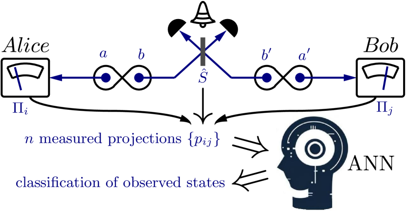
Figure 1: Conceptual diagram of quantum state classification from collective measurements using ANN. Two copies of a two-qubit state are subject to collective measurements yielding a vector of measurement outcomes $\{p_{ij}\}$. This feature vector of length $n$ is processed by the ANN that predicts the state’s class.

Evaluation of the quality of distributed quantum states becomes imperative in practical implementations of these communications networks. Furthermore, this assessment must be both highly accurate and rapid to avoid excessive consumption of expensive quantum resources. An elegant solution is found in the framework of collective measurements, applicable in the same geometric setup as entanglement swapping (refer to the conceptual diagram in Fig. 1) [23, 24, 25, 26, 27, 28]. While some quantum correlations can be unveiled through analytical calculations based on the outcomes of measurements performed in this setting, other, such as the negativity, are inaccessible this way [25]. A remedy lies in harnessing the predictive capability of artificial neural networks (ANN), renowned for their ability to predict quantum state properties even from incomplete measurements [29, 30, 31, 32, 33].

In this paper, we analyze the accuracy of detecting quantum state correlations through ANNs using collective measurements acquired in the entanglement swapping layout. Additionally, we evaluate the performance of ANNs under gradually reduced set of measurements determining the trade-off between accuracy and resource consumption [34]. We develop and test a method for optimization of this trade-off by employing the inner symmetry of the problem in two-qubit Hilbert space. Our focus is directed towards five important categories of quantum correlations and classification of quantum states into five corresponding and mutually exclusive groups based on the strongest quantum correlation categorized states can produce: Bell nonlocal states [3, 4, 5]; steerable [35, 36], but Bell local states; unsteerable states with fully entangled fraction (FEF) above the threshold of pure separable state (FEF $>\frac{1}{d}$, $d=2$ for qubits) [37, 38, 39, 26, 40]; entangled states not belonging to the previous class, i.e. FEF $\leq\frac{1}{d}$; and finally separable states (see summary in Table 1).

To enhance readability of the paper, the term entangled states refers to states that do not posses FEF above $\frac{1}{d}$. Similarly, the term steerable states designate states that are steerable, but not Bell non-local. The adoption of these five categories is justified by potential applications of nonlocal and steerable states in device-independent quantum cryptography and the entanglement as a resource unique to quantum technologies. Formal definitions are introduced in the next section.

Table 1: Hierarchy of quantum correlations used for state classification. Quantities used in the class definitions are formally introduced in Sec. 2.

Class	Description	Definition
sep	separable	$N=0$
ent	entangled	$N>0$ and FEFw= 0
FEF	fully ent. frac.	FEFw> 0 and $S_{3}=0$
steer	steerable	$S_{3}>0$ and $B=0$
Bell	Bell non-local	$B>0$

2 Quantum states generation and classification

To begin, we generated a collection of 160 million random two-qubit quantum states using the method outlined in [41, 42]. Following this, we employed analytical formulas based on the density matrix of each state to classify them [43]. The true labels $c$ acquired through this classification are utilized to subsequently train and test the ANN models later on. Negativity [44] was obtained from the eigenvalues of the partially transposed density matrix $\{\lambda_{i}\}=\mathrm{eigs}(\hat{\rho}^{\Gamma})$

$$N(\hat{\rho})=\sum_{i}|\lambda_{i}|-\lambda_{i}.$$ (1)

The remaining quantities were calculated using the correlation matrix $R=T^{T}T$, where

$$T_{ij}(\hat{\rho})=\mathrm{Tr}\left[\hat{\rho}(\sigma_{i}\otimes\sigma_{j})\right]$$ (2)

and $\sigma_{i}$ for $i\in[1,3]$ are Pauli matrices. According to its usual definition, FEF is expressed as the overlap between the tested state $\hat{\rho}$ and a maximally entangled state $|\Phi\rangle$ maximized over all maximally entangled states [38],

$$\mathrm{FEF}(\hat{\rho})\equiv\underset{|\Phi\rangle}{\max}\left\{\langle\Phi|\hat{\rho}|\Phi\rangle\right\}.$$

Instead of this standard definition, we use a more convenient fully entangled fraction witness,

$$\mathrm{FEF_{w}}(\hat{\rho})=\frac{1}{2}\mathrm{max}\left\{0,\mathrm{Tr}\sqrt{R}-1\right\},$$ (3)

which relates to FEF in a way that FEF_w$>0$ iff FEF $>{1\over d}$. Similarly, the Costa–Angelo 3-measurement steering [45] is calculated as

$$S_{3}(\hat{\rho})=\sqrt{\frac{1}{2}\mathrm{max}\left\{0,\mathrm{Tr}R-1\right\}}$$ (4)

and the Bell nonlocality [46, 47, 48],

$$B(\hat{\rho})=\sqrt{\mathrm{max}\{0,\mathrm{Tr}R-\mathrm{min}\left[\mathrm{eig}(R)\right]-1\}}.$$ (5)

For the labeling of generated states using the above-defined quantities see Tab. 1.

The correlation matrix $R$ can be efficiently obtained from a set of collective measurements implemented on two copies of the investigated state [49]

$$R_{ij}=\mathrm{Tr}\left[\hat{\rho}_{ab}\otimes\hat{\rho}_{a^{\prime}b^{\prime}}\hat{S}_{bb^{\prime}}\left(\sigma_{i}\otimes\sigma_{j}\right)_{aa^{\prime}}\right],$$ (6)

where $\hat{S}=1-4|\Psi^{-}\rangle\langle\Psi^{-}|$ and subscripts $\{a,b,a^{\prime},b^{\prime}\}$ denote subsystems of the first and second copy of the investigated state. $|\Psi^{-}\rangle$ is the maximally entangled singlet Bell state.

Importantly, negativity can not be calculated from the correlation matrix $R$ as it would require a more complex collective measurement strategy [25]. Eq. (6) stipulates that the correlation matrix $R$ can be obtained by applying 16 measurement configurations each corresponding to a combination of two von Neumann projectors applied to subsystems $a$ and $a^{\prime}$ (see conceptual scheme in Fig. 1) while subsystems $b$ and $b^{\prime}$ are always projected onto a singlet Bell state. For a detailed reasoning see subsection 5.2 of the Appendix.

One can further reduce the number of measurements by replacing the projectors based on Pauli matrices by the so-called minimal basis set [50]. The minimal basis set of projectors $\Pi_{i}$ for $i\in[0,3]$ is related to the Pauli matrices by a simple matrix transform $\Pi_{i}=\sum_{j}M_{ij}\sigma_{j}$ (assuming $\sigma_{0}=1$). For the details on the minimal basis projectors $\Pi_{i}$ and the matrix $M$, see subsection 5.2 in the Appendix. Replacing Pauli matrices in Eq. (6) by $\sum_{j}M_{ij}\Pi_{j}$ and considering symmetry of

$$p_{ij}=p_{ji}$$

for

$$p_{ij}=\mathrm{Tr}\left[\hat{\rho}_{ab}\otimes\hat{\rho}_{a^{\prime}b^{\prime}}\hat{S}_{bb^{\prime}}\left(\Pi_{i}\otimes\Pi_{j}\right)_{aa^{\prime}}\right]$$ (7)

decreases the number of measurement configurations needed to establish the correlation matrix $R$ to only 10 measurements. Graphical representation of the symmetry of measured quantities $p_{ij}$ as well as their unique numbering from 1 to 10 is presented in Fig. 2.

a) b)

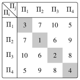
Figure 2: a) Labeling of collective two-qubit projections by indexes of $p_{ij}$ defined in Eq. (7). b) Feature ordering used in the higher-number projection strategy. Reduction is performed in the descending order of the values.

3 Implementation of the ANN models

We have implemented a series of ANN models to evaluate the performance of ANNs in classification of quantum states according to the hierarchy described in the preceding section and depicted in Tab. 1. To train and test our model without any bias, we have distilled a subset of the above-mentioned 160 million states so that each of the hierarchy classes appear with an equal probability of $1/5$. This means removing superfluous states belonging to more frequently occurring classes and, as a result, the size of the subset of states was reduced to about $1/3$, see subsection 5.1 and Fig. 7 in the Appendix. We refer to this procedure as equalization of the dataset. For all states within this subset, collective measurements outcomes $p_{ij}$ were calculated. Vectors of length $n$ composed of the values $F=\{p_{ij}\}$ represent the input features for the ANN models. In later sections we discuss the performance of the ANN models as function of the feature length $n$ as well as on the specific choice of the measurement configurations $p_{ij}$ leading to the best performance for a given value of $n$.

We have programmed all the ANN models using Pytorch Lightning [51]. Our ANN models consist of input and output layers of $n$ and 5 (number of classes) nodes respectively with two hidden layers in between each possessing 512 fully connected nodes. Each layer is preceded by a batch normalization layer to accelerate training [52]. Rectified linear activation function is used on every but the output layer, where a Softmax activation function is used instead. Loss is measured by means of the cross-entropy between the predicted $c^{\prime}$ and true labels $c$. The Adam optimizer [53] with learning rate of $10^{-4}$ is used to update the node weights upon training. Pytorch Lightning implementation of the models is available as Ancillary files.

The subset of input states was divided with the ratio of 12:3:1 to the training, validation and test set respectively. While a maximum number of training epochs was set to 4096, in practice the training was halted upon observing no improvement on the validation set for 10 consecutive epochs. Training started with the mini-batch size of $2^{12}=4096$ and then the models were finetuned with the mini-batch size of $2^{18}$ as recommended in Ref. [54]. Results on the validation set after training has stopped are used to establish the best performing model as well as the best suitable composition of the input feature vector $F$. This way, we have also established the hyper-parameters of our models presented in the preceding paragraph. Finally, the best performing model is tested on the independent test set to assess its true performance.

Upon testing, the test set was split to 12 subsets in order to estimate statistics of individual elements of the confusion matrix. Uncertainties typically scale as square roots of mean values corresponding to Poissonian distribution (see Fig. 3).

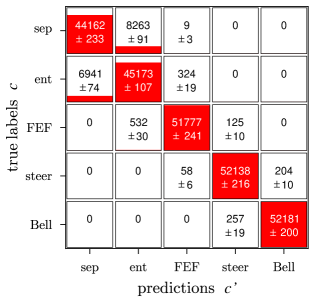
Figure 3: Confusion matrix for the feature vector $F$ of the full length $n=10$.

3.1 Benchmarking on full set of measurements

All correlations except for negativity can be analytically calculated from the correlation matrix $R$. We use this fact to asses performance of the ANN model when all the necessary information is provided to it, i.e. ANN is trained and tested on all $n=10$ measurement configurations $p_{ij}$ given by (7), that suffice to reconstruct the entire $R$ matrix. Predictions made by the ANN are accumulated into a confusion matrix CM. Element ${cc^{\prime}}$ of this matrix gives the number of states having the true label $c$ while being classified by the ANN as $c^{\prime}$. The overall accuracy of the model is given by

$$\mathcal{A}=\frac{\mathrm{Tr[CM]}}{\sum[\mathrm{CM}]}.$$ (8)

Meanwhile recall ${\cal R}$ represents the percentage of correctly classified states of a given category

$${\cal R}_{c}=\mathrm{prob}(c^{\prime}=c|c).$$ (9)

Precision ${\cal P}$, on the other hand, determines the probability that a state identified as $c^{\prime}$ actually belongs to the $(c=c^{\prime})$ class

$${\cal P}_{c^{\prime}}=\mathrm{prob}(c=c^{\prime}|c^{\prime}).$$ (10)

This means that recall, and precision is the percentage representation of the diagonal element of the confusion matrix in a given row and column, respectively. Finally, the $F_{1}$ score is calculated from both of these metrics according to the following formula which guarantees that it ranges from zero to one

$$F_{1}={2{\cal RP}\over{\cal R+P}}.$$ (11)

Figure 3 shows resulting confusion matrix when the ANN has access to all ten elements of the feature vector, $n=10$. This model was trained on a smaller 10M dataset ($10^{7}$ equalized random states) and then finally tuned on a bigger 50M dataset ($5\times 10^{7}$ equalized random states). Resulting $F_{1}$ score, recall ${\cal R}$ and precision ${\cal P}$ for identification of separable, entangled, FEF, steerable and Bell states are summarized in Tab. 2. The performance of the model can be evaluated by specifying the probability of the off-diagonal elements, which is in this case $6.38$ %. If we do not penalize misclassification between separable and entangled labels, which could not be analytically distinguished from the correlation matrix $R$, we are left with only $0.58$ % of off-diagonal elements. The average final accuracy reads $\mathcal{A}=93.62$ % or $99.42$ % when disregarding misclassification between separable and entangled states. The result of the classification based on the full set of measurements is sufficiently precise considering errors that are comparable to analytical classification assuming detection shot-noise. We can, at this point, start reducing the number of measurement configurations $n$ to make the procedure less resource demanding.

Table 2: Recall ${\cal R}$, precision ${\cal P}$ and the $F_{1}$ score calculated from the confusion matrix in Fig. 3.

	sep	ent	FEF	steer	Bell
${\cal R}(\%)$	84.22 $\pm$ 0.16	86.15 $\pm$ 0.13	98.74 $\pm$ 0.06	99.50 $\pm$ 0.02	99.51 $\pm$ 0.04
${\cal P}(\%)$	86.42 $\pm$ 0.14	83.70 $\pm$ 0.15	99.25 $\pm$ 0.04	99.27 $\pm$ 0.04	99.61 $\pm$ 0.02
$F_{1}(\%)$	85.31 $\pm$ 0.11	84.91 $\pm$ 0.10	99.00 $\pm$ 0.04	99.39 $\pm$ 0.02	99.56 $\pm$ 0.02

3.2 Finding optimal strategy for measurement reduction

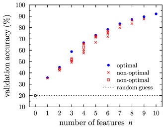
Figure 4: Validation accuracy for 10M equalized dataset as a function of the length of feature vector used for training the model. This plot indicates optimality of the selected reduction strategy (blue points). When the reduction of feature elements does not follow the outlined rules, the resulting accuracy is suboptimal (red symbols).

First, we have conducted a preliminary testing on a smaller 10M dataset to verify optimality of the procedure of measurement reduction (reduction of the length $n$ of the input feature vector). We identify two optimal reduction strategies; one for higher number of projections ($n\geq 5$) and the second for smaller values of $n<5$. Both strategies have their specific physical reasoning based on the inner symmetry of the collective measurements. In case of the first strategy, the ordering of ten elements of the feature vector ($F=\{1,\ldots,10\}$) is depicted on the Fig. 2b). The element number 10 is removed as the first then element 9 and so on till $n=5$. Optimal reduction in this range of the values of $n$ is governed by two rules: (i) It is advantageous to retain the four diagonal feature elements $p_{ii}$ for as long as possible, as they contain more information than the six off-diagonal elements. (ii) If possible, it is favorable not to cumulate canceled elements on a single row or column.

Continuing with this strategy for $n<5$ would result in suboptimal solutions as depicted by red squares in the Fig. 4, for $n\in\{2,3,4\}$. Therefore, as of $n=4$, we switch to the second strategy motivated by the Collectibility witness [24]. In the next two steps ($n=4$ and $n=3$) we still keep one off-diagonal element $p_{ij}$ together with its two corresponding diagonal counterparts $p_{ii}$ and $p_{jj}$. In case of $n=4$ we add another diagonal element $p_{kk}$, $k\neq i$ nor $j$. This corresponds to the measurement of the Collectibility for a pure state ($n=3$ case) and for a mixed state ($n=4$ case). It is interesting, that for $n=2$ the optimal strategy is to remove all diagonal elements keeping two off-diagonal elements $p_{ij}$ and $p_{kl}$, where indices $\{i,j,k,l\}$ are exclusively different numbers. Finally, for $n=1$ it is again slightly more convenient to keep one diagonal element. More details are presented in subsection 5.3 of the Appendix.

Note that in the case of having no measurements at all ($n=0$), the accuracy of estimation would decrease to 20 %, i.e. a random guess strategy.

Correctness of our assertion is verified by numerical testing of several ANN models operating on various feature vectors (see Fig. 4). All the models trained with the same symmetry of input feature vectors end with similar accuracy with a deviation of 0.7 %. This contrasts with non-optimal reduction strategies that can render accuracies more then 10 % smaller. Note that there exist other established strategies for feature reduction [23, 55], but our approach is favoured because of its clear physical interpretation.

3.3 Final results obtained following the optimal reduction strategy

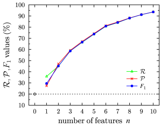
Figure 5: Results of the model trained on the 50M dataset using optimal sequences of features of given lengths $n$. The points shown represent mean values of recall ${\cal R}$, precision ${\cal P}$ and the $F_{1}$ score over all categories.

Table 3: $F_{1}$ scores for all 5 states’ classes and the overall accuracy $\mathcal{A}$ as functions of feature vector length $n$.

$n$	$F_{1}$ (%)					$\mathcal{A}$ (%)
	sep	ent	FEF	steer	Bell
10	85.31 $\pm$ 0.11	84.91 $\pm$ 0.10	99.00 $\pm$ 0.04	99.39 $\pm$ 0.02	99.56 $\pm$ 0.02	93.62 $\pm$ 0.24
9	84.35 $\pm$ 0.11	80.94 $\pm$ 0.11	94.59 $\pm$ 0.07	97.56 $\pm$ 0.05	98.54 $\pm$ 0.04	91.17 $\pm$ 0.25
8	82.98 $\pm$ 0.11	77.01 $\pm$ 0.11	88.83 $\pm$ 0.10	94.54 $\pm$ 0.07	97.13 $\pm$ 0.04	88.05 $\pm$ 0.23
7	80.20 $\pm$ 0.14	72.08 $\pm$ 0.12	82.09 $\pm$ 0.12	91.03 $\pm$ 0.09	95.42 $\pm$ 0.07	84.05 $\pm$ 0.23
6	77.37 $\pm$ 0.13	67.32 $\pm$ 0.12	76.90 $\pm$ 0.13	88.51 $\pm$ 0.09	94.32 $\pm$ 0.07	80.72 $\pm$ 0.22
5	74.19 $\pm$ 0.14	60.10 $\pm$ 0.12	64.96 $\pm$ 0.15	79.66 $\pm$ 0.11	90.00 $\pm$ 0.09	73.65 $\pm$ 0.20
4	71.58 $\pm$ 0.13	53.91 $\pm$ 0.12	54.88 $\pm$ 0.13	69.64 $\pm$ 0.12	82.73 $\pm$ 0.13	66.37 $\pm$ 0.17
3	67.53 $\pm$ 0.15	44.67 $\pm$ 0.16	45.88 $\pm$ 0.11	60.33 $\pm$ 0.12	74.50 $\pm$ 0.15	58.61 $\pm$ 0.17
2	58.23 $\pm$ 0.15	39.86 $\pm$ 0.14	35.11 $\pm$ 0.16	39.99 $\pm$ 0.20	52.56 $\pm$ 0.18	45.05 $\pm$ 0.18
1	52.23 $\pm$ 0.14	35.43 $\pm$ 0.11	0	13.07 $\pm$ 0.09	46.85 $\pm$ 0.14	35.82 $\pm$ 0.13

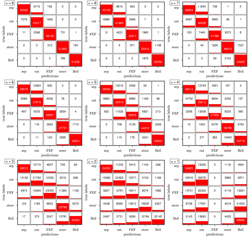
Figure 6: Confusion matrices as functions of the feature vector length $n$. Confusion matrix for $n=10$ is shown in Fig. 3.

Once the optimal feature-reduction procedure has been identified and verified, we have proceeded with the final ANN training on the full 50M dataset. Figure 5 shows results obtained when reducing the length $n$ of the feature vector from 10 down to 1. The resulting decrease of the $F_{1}$ scores for all categories of states is also listed in Tab. 3. The trend is similar to that for the validation set (Fig. 4). Only the resulting accuracy is slightly better for 50M dataset.

Figure 6 presents individual confusion matrices for various values of $n$ from which the precision and recall are calculated. Even though it is impossible to distinguish separable and entangled states by means of analytical calculations, the ANNs achieve this task, albeit with reduced accuracy. This figure also shows gradual spreading of the diagonal elements of the confusion matrix when reducing the number of measurements. Given the equal representation of all classes in the dataset, the sum over any row in the CM yields a constant value. The biggest value is found on the diagonal and it gradually decreases with the decreasing number of measurements $n$. This trend continues down to $n=2$, but for $n=1$ we observe a binarization of the classification splitting the states into two extreme groups: weakly correlated (i.e. separable and entangled) and strongly correlated (i.e. steerable and nonlocal). No state is classified as FEF class. This effect is also witnessed by spreading of precision and recall values for $n=1$ (see Fig. 5).

4 Conclusions

This paper has demonstrated the practicality and effectiveness of using ANNs for classification of quantum correlations in a layout typical for entanglement-swapping networks. To optimize resource utilization, we implemented several key measures. Initially, we adopted the minimal basis set, thereby diminishing the required number of measurement configurations for analytical classification from 16 to 10. Subsequently, we identified and numerically tested the optimal measurement reduction strategy, leveraging the inherent symmetry of the task. This ultimately enabled us to train ANN models with varying numbers of measurement projections and assess the resulting precisions, recalls, accuracies, and $F_{1}$ scores.

To evaluate the performance of the ANN-based classification, we first started with a model trained using the entire set of 10 measurement configurations and benchmarked its accuracy against analytical calculations. The ANN model reached a classification accuracy of 99.42 % when allowing for misclassification between separable and entangled states. It is important to note that the calculation of negativity, necessary for the proper classification of these two categories, cannot be performed analytically based on the available measurements. The achieved accuracy of the ANN models is quite comparable to a perfect analytical classification assuming inevitable measurement errors in a practical environment. Furthermore, the ANN model demonstrated the capability to label separable and entangled states with an accuracy of 85.46 %, a task unfeasible through conventional analytical calculations. This underscores the benefits of the ANN classification over the analytical approach.

The adaptability of the ANNs enables the implementation of classification models using an incomplete set of projections – a challenge unattainable by analytical formulae. To observe the diminishing performance of the ANN models, we reduced the number of measurement configurations from 10 to 1. The performance decline is gradual, with an accuracy of 73.65 % achieved with half of the measurements ($n=5$). Finally, an accuracy of 35.82 % is obtained with just one single measurement. It is worth noting that a random guessing approach, without any measurements, would yield an accuracy of 20 %.

Classifying quantum correlations is a crucial challenge in the field of practical quantum communications networks, particularly when considering the security implications associated with individual correlations. Consequently, we believe that our findings make a useful contribution to the ongoing endeavors aimed at advancing quantum communications toward practical deployment. Furthermore, the method we have outlined introduces novel research opportunities in the detection of quantum correlations, addressing, thus, an intriguing and open fundamental problem in the field.

5 Appendix

5.1 Equalization of the dataset

To train and test the ANN models, we first generate a random set of states that are evenly distributed in the space of two-qubit states, as was described in Refs. [41, 42]. Preparation of random datasets is schematically depicted in Fig. 7. Because individual categories of states are not equivalently represented in the raw random dataset, it was necessary to distill an equally balanced (equalized) set. The equalization is done by reducing the number of more populated categories to the number corresponding to the least populated category, which is steerable states. This equalized set is then divided into three parts. The first part is used to train the model (the training set). The second part of these random equalized states is utilized for validation to stop training in time (prevent overfitting) and compare the performance of various models with different hyperparameters (especially the composition of the input feature vector, see Subsec. 3.2). The model that has been the most successful in terms of accuracy in recognizing states is chosen for testing on the final test set of random equalized states.

5.2 Minimal required measurements

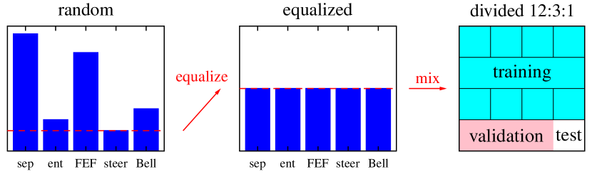
Figure 7: Scheme of the dataset preparation.

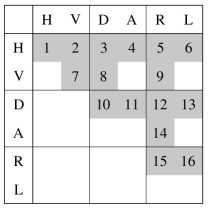
Figure 8: Sixteen required von Neumann projections to obtain the correlation matrix $R$ from Pauli measurements. Other not numbered measurements can be derived/deduced using symmetry considerations. Symbols $\{H,V,D,A,R,L\}$ stand for the six eigenstates of the Pauli matrices labelled following the traditional symbolism of polarization optics as horizontal, vertical, diagonal, anti-diagonal, right and left circular, respectively.

Traditionally, the correlation matrix $R$ is expressed in terms of the Pauli matrices [see Eq. (6)]. Each Pauli matrix consists of two von Neumann projectors, hence measuring expectation values of all these matrices on a single qubit requires to perform 6 projective measurements. In case of two qubits, the total number of projective measurements amounts to $6\times 6=36$ as illustrated in Fig. 8. This number of measurements can be reduced to 16 due to the symmetry of the correlation matrix $R_{ij}=R_{ji}$ and also due the completeness relation

$$\sigma^{+}_{i}\sigma^{+}_{j}+\sigma^{+}_{i}\sigma^{-}_{j}+\sigma^{-}_{i}\sigma^{+}_{j}+\sigma^{-}_{i}\sigma^{-}_{j}=1,$$ (12)

where $\sigma^{\pm}_{i}$ are the von Neumann projectors such that $\sigma_{i}=\sigma^{+}_{i}-\sigma^{-}_{i}$, where $\sigma_{i}$ is the $i$-th Pauli matrix. Note that the 16th measurement is needed assuming that the overall count rate is not known in advance.

In order to obtain complete information about a single-qubit state, it is, however, not necessary to perform 6, but only 4 projection measurements of the minimal basis set $\{\Pi_{i}\}$ [50]. The directions of the minimal basis projection measurements are represented by vertices of a tetrahedron inside the Bloch sphere. Applying this minimal basis set to a two-qubit state requires to perform $4\times 4=16$ projective measurements. All performed projections can be written in a table, where the rows represent projections on one qubit, and the columns on the other one. Projections performed in the same direction on both qubits are represented by diagonal elements marked grey in the table in Fig. 2. Due to the symmetry of $R$, only diagonal and upper off-diagonal elements are unique, this reduces the total number of two-qubit projections to 10.

The correlation matrix $R$ can be easily obtained from the minimal basis projections $\Pi_{i}$ using the linear relation

$$\Pi_{i}=\sum_{j}M_{ij}\sigma_{j},\quad i,j\in[0,3],\quad\sigma_{0}=1,$$

where

$$M={1\over 4}\left(\begin{array}[]{rrrr}1&s&s&s\\ 1&s&-s&-s\\ 1&-s&s&-s\\ 1&-s&-s&s\\ \end{array}\right),\quad s={1\over\sqrt{3}}.$$

5.3 Selected order of the features

Here we describe our selection of feature ordering following the rules described in sec. 3.2. The optimality of our reduction strategy can also be deduced from Fig. 4, where the validation accuracy is plotted as a function of the number of the input features. Firstly, for $n\geq 5$ it is advantageous to retain the diagonal feature elements for as long as possible as they contain more information than the off-diagonal elements. When transitioning from ten measurements to nine, the selection of any off-diagonal element is arbitrary, so there are six equivalently correct possibilities. We remove element $p_{13}$. After that, for $n=8$, the next removed element is uniquely determined due to symmetry. It must be the element $p_{24}$. Removing two elements that intersect on the same row or column would be a mistake leading to unnecessary reduction in accuracy. In the third step ($n=7$), we can again remove any remaining off-diagonal element arbitrarily. We selected $p_{34}$, so in the next fourth step ($n=6$) we must remove $p_{12}$. At this point we have all diagonal elements and exactly one off-diagonal measurement remaining in each row and each column.

Subsequently for $n=5$, we remove one of the remaining off-diagonal elements ($p_{23}$) and the last remaining off-diagonal element determines the next course of action.

Continuing the reduction for $n<5$, we keep the off-diagonal element $p_{14}$ so we have to keep $p_{11}$ and $p_{44}$ when reducing to $n=4$ and $n=3$. In case of $n=4$ one additional diagonal element $p_{33}$ is selected to complement $p_{14}$, $p_{11}$ and $p_{44}$.

For $n=2$ we have to select two off-diagonal elements, i.e. $p_{14}$ and $p_{23}$. In the last step with only one measurement, it is favourable to employ a diagonal element: we select $p_{22}$. In the case of having no measurements at all, the accuracy of estimation would be inherently only $1/5=20$ % corresponding to a random guess.

References

- [1] P. A. M. Dirac. “The principles of quantum mechanics, 3rd ed.”. Oxford, The Clarendon Press, UK. (1948). url: https://archive.org/details/principlesquantummechanics1stdirac1930.
- [2] M. A. Nielsen and I. L. Chuang. “Quantum computation and quantum information”. Cambridge University Press, Cambridge, UK. (2000).
- [3] J. S. Bell. “On the Einstein Podolsky Rosen paradox”. Physics Physique Fizika 1, 195–200 (1964).
- [4] John F. Clauser, Michael A. Horne, Abner Shimony, and Richard A. Holt. “Proposed experiment to test local hidden-variable theories”. Phys. Rev. Lett. 23, 880–884 (1969).
- [5] Alain Aspect, Philippe Grangier, and Gérard Roger. “Experimental tests of realistic local theories via Bell’s theorem”. Phys. Rev. Lett. 47, 460–463 (1981).
- [6] Alain Aspect, Jean Dalibard, and Gérard Roger. “Experimental test of Bell’s inequalities using time-varying analyzers”. Phys. Rev. Lett. 49, 1804–1807 (1982).
- [7] Gregg Jaeger. “Quantum information: an overview”. Springer. (2010).
- [8] Dik Bouwmeester, Jian-Wei Pan, Klaus Mattle, Manfred Eibl, Harald Weinfurter, and Anton Zeilinger. “Experimental quantum teleportation”. Nature 390, 575–579 (1997).
- [9] Jian-Wei Pan, Dik Bouwmeester, Harald Weinfurter, and Anton Zeilinger. “Experimental entanglement swapping: Entangling photons that never interacted”. Phys. Rev. Lett. 80, 3891–3894 (1998).
- [10] Artur K. Ekert. “Quantum cryptography based on Bell’s theorem”. Phys. Rev. Lett. 67, 661–663 (1991).
- [11] Giuseppe Castagnoli. “On the relation between quantum computational speedup and retrocausality”. Quanta 5, 34–52 (2016).
- [12] David Layden, Guglielmo Mazzola, Ryan V. Mishmash, Mario Motta, Pawel Wocjan, Jin-Sung Kim, and Sarah Sheldon. “Quantum-enhanced Markov chain Monte Carlo”. Nature 619, 1476–4687 (2023).
- [13] Alastair A. Abbott and Cristian S. Calude. “Understanding the quantum computational speed-up via de-quantisation”. In DCM. (2010). url: https://api.semanticscholar.org/CorpusID:6173695.
- [14] C. L. Degen, F. Reinhard, and P. Cappellaro. “Quantum sensing”. Rev. Mod. Phys. 89, 035002 (2017).
- [15] Luca Pezzè, Augusto Smerzi, Markus K. Oberthaler, Roman Schmied, and Philipp Treutlein. “Quantum metrology with nonclassical states of atomic ensembles”. Rev. Mod. Phys. 90, 035005 (2018).
- [16] John F. Barry, Jennifer M. Schloss, Erik Bauch, Matthew J. Turner, Connor A. Hart, Linh M. Pham, and Ronald L. Walsworth. “Sensitivity optimization for NV-diamond magnetometry”. Rev. Mod. Phys. 92, 015004 (2020).
- [17] Ernest Y.-Z. Tan, Pavel Sekatski, Jean-Daniel Bancal, René Schwonnek, Renato Renner, Nicolas Sangouard, and Charles C.-W. Lim. “Improved DIQKD protocols with finite-size analysis”. Quantum 6, 880 (2022).
- [18] Yi-Zheng Zhen, Yingqiu Mao, Yu-Zhe Zhang, Feihu Xu, and Barry C. Sanders. “Device-independent quantum key distribution based on the Mermin-Peres magic square game”. Phys. Rev. Lett. 131, 080801 (2023).
- [19] Jun Xin, Xiao-Ming Lu, Xingmin Li, and Guolong Li. “One-sided device-independent quantum key distribution for two independent parties”. Opt. Express 28, 11439–11450 (2020).
- [20] H.-J. Briegel, W. Dür, J. I. Cirac, and P. Zoller. “Quantum repeaters: The role of imperfect local operations in quantum communication”. Phys. Rev. Lett. 81, 5932–5935 (1998).
- [21] B. C. Jacobs, T. B. Pittman, and J. D. Franson. “Quantum relays and noise suppression using linear optics”. Phys. Rev. A 66, 052307 (2002).
- [22] Artur Barasiński, Antonín Černoch, and Karel Lemr. “Demonstration of controlled quantum teleportation for discrete variables on linear optical devices”. Phys. Rev. Lett. 122, 170501 (2019).
- [23] Łukasz Rudnicki, Paweł Horodecki, and Karol Życzkowski. “Collective uncertainty entanglement test”. Phys. Rev. Lett. 107, 150502 (2011).
- [24] Łukasz Rudnicki, Zbigniew Puchała, Paweł Horodecki, and Karol Życzkowski. “Collectibility for mixed quantum states”. Phys. Rev. A 86, 062329 (2012).
- [25] Karol Bartkiewicz, Grzegorz Chimczak, and Karel Lemr. “Direct method for measuring and witnessing quantum entanglement of arbitrary two-qubit states through Hong-Ou-Mandel interference”. Phys. Rev. A 95, 022331 (2017).
- [26] Karol Bartkiewicz, Karel Lemr, Antonín Černoch, and Adam Miranowicz. “Bell nonlocality and fully entangled fraction measured in an entanglement-swapping device without quantum state tomography”. Phys. Rev. A 95, 030102 (2017).
- [27] Karol Bartkiewicz and Grzegorz Chimczak. “Two methods for measuring Bell nonlocality via local unitary invariants of two-qubit systems in Hong-Ou-Mandel interferometers”. Phys. Rev. A 97, 012107 (2018).
- [28] Vojtěch Trávníček, Karol Bartkiewicz, Antonín Černoch, and Karel Lemr. “Experimental measurement of a nonlinear entanglement witness by hyperentangling two-qubit states”. Phys. Rev. A 98, 032307 (2018).
- [29] Marco Tomamichel and Renato Renner. “Uncertainty relation for smooth entropies”. Phys. Rev. Lett. 106, 110506 (2011).
- [30] Dominik Koutný, Laia Ginés, Magdalena Moczała-Dusanowska, Sven Höfling, Christian Schneider, Ana Predojević, and Miroslav Ježek. “Deep learning of quantum entanglement from incomplete measurements”. Science Advances 9, eadd7131 (2023).
- [31] Jan Roik, Karol Bartkiewicz, Antonín Černoch, and Karel Lemr. “Accuracy of entanglement detection via artificial neural networks and human-designed entanglement witnesses”. Phys. Rev. Appl. 15, 054006 (2021).
- [32] Jan Roik, Karol Bartkiewicz, Antonín Černoch, and Karel Lemr. “Entanglement quantification from collective measurements processed by machine learning”. Physics Letters A 446, 128270 (2022).
- [33] Alexander C.B. Greenwood, Larry T.H. Wu, Eric Y. Zhu, Brian T. Kirby, and Li Qian. “Machine-learning-derived entanglement witnesses”. Phys. Rev. Appl. 19, 034058 (2023).
- [34] M. Deisenroth, A. Faisal, and C. Ong. “Mathematics for machine learning”. Cambridge University Press, UK. (2020).
- [35] H. M. Wiseman, S. J. Jones, and A. C. Doherty. “Steering, entanglement, nonlocality, and the Einstein-Podolsky-Rosen paradox”. Phys. Rev. Lett. 98, 140402 (2007).
- [36] Xiao-Gang Fan, Huan Yang, Fei Ming, Dong Wang, and Liu Ye. “Constraint relation between steerability and concurrence for two-qubit states”. Ann. der Physik 533, 2100098 (2021).
- [37] Charles H. Bennett, David P. DiVincenzo, John A. Smolin, and William K. Wootters. “Mixed-state entanglement and quantum error correction”. Phys. Rev. A 54, 3824 (1996).
- [38] J. Grondalski, D.M. Etlinger, and D.F.V. James. “The fully entangled fraction as an inclusive measure of entanglement applications”. Physics Letters A 300, 573–580 (2002).
- [39] Ming-Jing Zhao, Zong-Guo Li, Shao-Ming Fei, and Zhi-Xi Wang. “A note on fully entangled fraction”. Journal of Physics A: Mathematical and Theoretical 43, 275203 (2010).
- [40] Tapaswini Patro, Kaushiki Mukherjee, Mohd Asad Siddiqui, Indranil Chakrabarty, and Nirman Ganguly. “Absolute fully entangled fraction from spectrum”. The European Physical Journal D 76, 127 (2022).
- [41] Marcin Pozniak, Karol Zyczkowski, and Marek Kus. “Composed ensembles of random unitary matrices”. Journal of Physics A: Mathematical and General 31, 1059 (1998).
- [42] Jonas Maziero. “Random sampling of quantum states: a survey of methods”. Brazilian Journal of Physics 45, 575–583 (2015).
- [43] Shilan Abo, Jan Soubusta, Kateřina Jiráková, Karol Bartkiewicz, Antonín Černoch, Karel Lemr, and Adam Miranowicz. “Experimental hierarchy of two-qubit quantum correlations without state tomography”. Scientific Reports 13, 8564 (2023).
- [44] K. Życzkowski, P. Horodecki, A. Sanpera, and M. Lewenstein. “Volume of the set of separable states”. Phys. Rev. A 58, 883–892 (1998).
- [45] A. C. S. Costa and R. M. Angelo. “Quantification of Einstein-Podolski-Rosen steering for two-qubit states”. Phys. Rev. A 93, 020103 (2016).
- [46] R. Horodecki, P. Horodecki, and M. Horodecki. “Violating Bell inequality by mixed states: necessary and sufficient condition”. Phys. Lett. A 200, 340–344 (1995).
- [47] A. Miranowicz. “Violation of Bell inequality and entanglement of decaying Werner states”. Phys. Lett. A 327, 272–283 (2004).
- [48] Huan Yang, Fa Zhao, Xiao-Gang Fan, Zhi-Yong Ding, Dong Wang, Xue-Ke Song, Hao Yuan, Chang-Jin Zhang, and Liu Ye. “Estimating quantum steering and Bell nonlocality through quantum entanglement in two-photon systems”. Opt. Express 29, 26822 (2021).
- [49] Karol Bartkiewicz, Bohdan Horst, Karel Lemr, and Adam Miranowicz. “Entanglement estimation from Bell inequality violation”. Phys. Rev. A 88, 052105 (2013).
- [50] Jaroslav Řeháček, Berthold-Georg Englert, and Dagomir Kaszlikowski. “Minimal qubit tomography”. Phys. Rev. A 70, 052321 (2004).
- [51] Adam Paszke, Sam Gross, Francisco Massa, Adam Lerer, James Bradbury, Gregory Chanan, Trevor Killeen, Zeming Lin, Natalia Gimelshein, Luca Antiga, Alban Desmaison, Andreas Kopf, Edward Yang, Zachary DeVito, Martin Raison, Alykhan Tejani, Sasank Chilamkurthy, Benoit Steiner, Lu Fang, Junjie Bai, and Soumith Chintala. “Pytorch: An imperative style, high-performance deep learning library”. In Advances in Neural Information Processing Systems 32. Pages 8024–8035. Curran Associates, Inc. (2019). url: http://papers.neurips.cc/paper/9015-pytorch-an-imperative-style-high-performance-deep-learning-library.pdf.
- [52] Sergey Ioffe and Christian Szegedy. “Batch normalization: Accelerating deep network training by reducing internal covariate shift” (2015). arXiv:1502.03167.
- [53] Diederik P. Kingma and Jimmy Ba. “Adam: A method for stochastic optimization” (2017). arXiv:1412.6980.
- [54] Samuel L. Smith, Pieter-Jan Kindermans, Chris Ying, and Quoc V. Le. “Don’t decay the learning rate, increase the batch size” (2018). arXiv:1711.00489.
- [55] Scott M Lundberg and Su-In Lee. “A unified approach to interpreting model predictions”. In I. Guyon, U. V. Luxburg, S. Bengio, H. Wallach, R. Fergus, S. Vishwanathan, and R. Garnett, editors, Advances in Neural Information Processing Systems 30. Pages 4765–4774. Curran Associates, Inc. (2017). url: http://papers.nips.cc/paper/7062-a-unified-approach-to-interpreting-model-predictions.pdf.