Approximating maximum independent set on Rydberg atom arrays using local detunings

Abstract

Rydberg atom arrays are among the most promising quantum simulating platforms due to their scalability and long coherence time. From the perspective of combinatorial optimization, they are intrinsic solver for the maximum independent set problem because of the resemblance between the Rydberg Hamiltonian and the cost function of the maximum independent set problem. In this paper, we suggest a strategy to approximate maximum independent sets by adjusting local detunings on the Rydberg Hamiltonian according to each vertex’s vertex support, which is a quantity that represents connectivity between vertices. By doing so, we explicitly reflect on the Rydberg Hamiltonian the potential probability that each vertex will be included in maximum independent sets. Our strategy reduces an error rate three times for the checkerboard graphs with defects when the adiabaticity is enough. Our strategy also decreases the error rate for random graphs of density 3.0, even when the adiabaticity is relatively insufficient. Moreover, we harness our strategy to raise the fidelity between the evolved quantum state and a 2D cat state on a square lattice, showing that our strategy helps to prepare a quantum many-body ground state.

I Introduction

Quantum adiabatic algorithm (QAA) stands out as one of the highly feasible algorithms soon due to its simplicity AL18 . It harnesses the adiabatic theorem to obtain a ground state of the target Hamiltonian by gradually transitioning from the ground state of a specific manageable Hamiltonian RC02 ; FGG02 ; EWL+21 . Interestingly, one can acquire solutions for combinatorial optimization problems by letting the target Hamiltonian be a cost function of the combinatorial optimization problems HP00 ; CFGG02 . They are practical in real life, but most cases are in the regime of NP-hard class, in which no known classical polynomial algorithm exists S05 ; FGG+01 .

Thanks to its simplicity, QAA has been successfully implemented on various platforms such as superconductors RMM+09 , trapped ions QLR+09 and Rydberg atom arrays  SSW+21 ; OLK+19 . In situations where the cost function of the problems naturally resembles the hardware’s Hamiltonian, QAA offers a significant advantage in terms of scalability, only requiring sufficient Hamiltonian evolution EWL+21 ; SSW+21 . One of the most prominent examples of this alignment in combinatorial optimization problems is the maximum independent set (MIS) problem on Rydberg atom arrays due to their intrinsic resemblance PWZCL18 ; PWZCL18+ , which serves as the primary focus of our work.

The MIS is the largest subset of the whole vertices set in which no two vertices are connected. The problem of finding MIS is NP-hard in the worst case. The MIS has various practical applications WLG+22 such as wireless networks WAJ10 and massive data sets B03 . One of the most important subclasses of the MIS is the MIS on a unit-disk graph, where finding it is also NP-hard in the worst case CCJL90 . Rydberg atom arrays are especially good at describing the MIS problem on a unit-disk graph cost function by realizing the independence constraint via the Rydberg blockade mechanism. This mechanism results from the robust van der Waals interaction between two Rydberg states, which are highly excited states of atoms WLT+21 .

There are multiple studies to identify MIS through the Rydberg atom arrays are underway, such as encoding arbitrarily connected graphs into Rydberg atom arrays by adding ancillary qubits KKH+22 ; NLW+23 or mapping the Rydberg Hamiltonian onto the other tractable Hamiltonian GMOS23 . Furthermore, protocols to enhance its speed by introducing a new term to the Rydberg Hamiltonian were also proposed SWM+23 ; CCL+23 . Recently, Ebadi et al. EKC+22 have made significant strides by experimentally demonstrating superlinear speedup compared to the classical method, finding MIS on unit-disk graphs of up to 289 qubits using Rydberg atom arrays. (We notice that Ref. ASM+23 proposed a new classical strategy competitive with the speed of the quantum method in Ref. EKC+22 .)

Nevertheless, an approximation scheme designed explicitly for the MIS problem on the Rydberg Hamiltonian does not exist. Approximating MIS for general graphs is a challenging task, which has a polynomial time algorithm capable of finding an approximate solution within a polynomial fraction of the exact solution (Fall into APX-complete class) B03 . Regarding a unit-disk graph, approximated solutions within a desired fraction of exact solutions can be obtained in polynomial time (Fall into the PTAS class). However, practical limitation arises when aiming to achieve a valuable fraction of the exact solutions in this case DDK+15 . Therefore, the need for a more efficient approximation scheme tailored to the Rydberg atom arrays arises.

In this study, we present a strategy designed to find approximated solutions of MIS problem on a unit-disk graph by utilizing local detunings of the Rydberg Hamiltonian during the QAA. Our approach incorporates the ‘vertex support’ concept introduced in Ref. BSK10 to estimate the potential probability that each vertex will be included in MIS. Estimated potentials are assigned to each atom’s detuning magnitude during the adiabatic evolution. This process encourages atoms, more likely to be included in MIS, to be in the Rydberg state at the end of evolution. We optimize the acceptance degree of vertex support in our strategy and compare its performance to the case without considering vertex support. Our strategy successfully reduced error rates for two types of graphs: checkerboard graphs with defects and random graphs. The error rate was reduced three times for checkboard graphs with defects when the adiabaticity was enough. For random graphs with density of 3.0, our strategy reduced the error rate even when the adiabaticity was insufficient, which implies that our strategy is applicable to larger graphs, which are hard to deal with classical computers.

Following the above process, we can obtain knowledge about the arrangement of the ground states of the final Hamiltonian. However, we are uncertain whether we obtain an actual physical quantum ground state because a lack of information about ground states requires classical postprocessing after evolution in our process. On the other hand, if we know the ground state of some special systems BSK+17 ; EWL+21 ; SSW+21 , we can maximize the probability of obtaining this ground state, harnessing the vertex support concept as a connectivity measure. By doing so, we increase the fidelity of a 2D cat state OLK+19 from 0.68 to 0.90, which is a quantum superposition of two opposite states.

This paper is organized as follows. In Sec. II, we supply the definitions of the Rydberg Hamiltonian and a MIS cost function, which are the main models in this paper. Additionally, we provide an adiabatic schedule used in this paper and a definition of the vertex support. Next, sec. III starts with our strategy which describes how to adjust local detunings according to each vertex’s vertex supports. After that, numerical simulations are depicted, evaluating our strategy’s performance on checkerboard graphs with sufficient adiabaticity, random graphs with density of 3.0, and random graphs with density of 3.0 that lack adiabaticity. At the end of this section, we analyze the effect of our strategy while preparing a 2D cat state on a $4\times 4$ square lattice. Finally, we provide summaries and discussions in IV.

II Models and Methods

II.1 Rydberg Hamiltonian and MIS cost function

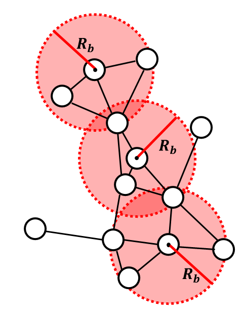
(a)

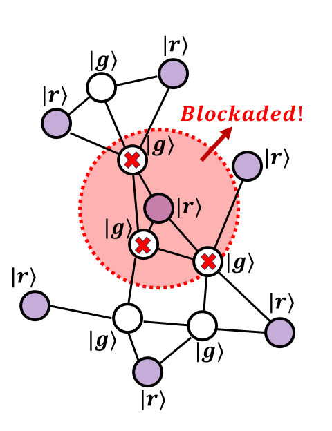
(b)

Figure 1: (a) Two vertices are connected when one vertex is within the Rydberg blockade radius $R_{b}$ of another, which allows us to regard the configuration of atoms as the unit-disk graph. The red circles denote the Rydberg blockade range of an atom. (b) Only one atom can be excited to a Rydberg state in a Rydberg blockade radius by the Rydberg blockade mechanism. The color of Rydberg state atoms is purple, and the ground state atom is white.

Consider a system consisting of $N$ atoms which satisfy the Rydberg Hamiltonian. For the Rydberg Hamiltonian, let us denote the $i$-th Rydberg atom array’s ground state as $|g_{i}\rangle$, the Rydberg state as $|r_{i}\rangle$, and the Rydberg number operator as $\hat{n}_{i}:=|r_{i}\rangle\langle r_{i}|$. The Rydberg Hamiltonian can be decomposed as follows,

$$H_{\mathrm{Ryd}}=H_{\Omega}+H_{\Delta}+H_{V},$$ (1)

where the $H_{\Omega}$ is the driving part, the $H_{\Delta}$ is the detuning part, and the $H_{V}$ is the interaction part. The details of each Hamiltonian is as follows:

$$H_{\Omega}(t)=\sum_{j=1}^{N}\cfrac{\Omega_{j}(t)}{2}(e^{i\phi_{j}(t)}|g_{j}\rangle\langle r_{j}|+e^{-i\phi_{j}(t)}|r_{j}\rangle\langle g_{j}|),$$ (2)

$$H_{\Delta}(t)=-\sum_{j=1}^{N}\Delta_{j}(t)\hat{n}_{j},\quad{\textnormal{and}}$$ (3)

$$H_{V}=\sum_{j<k}V_{jk}\hat{n}_{j}\hat{n}_{k}.$$ (4)

The symbols $\Omega_{j}$, $\phi_{j}$, and $\Delta_{j}$ characterize the Rabi frequency, the phase of the laser, and the driving laser field’s detuning of the j-th atom, respectively. Moreover, $V_{jk}=C_{6}/|\vec{r}_{j}-\vec{r}_{k}|^{6}$ is the Rydberg interaction, a type of van der Waals interaction between two Rydberg states where $C_{6}$ represents the interaction constant. We set $C_{6}$ as $2\pi\times 862690~{}\text{MHz}~{}\mu m^{6}$ in this work. This intensive interaction creates the Rydberg blockade phenomenon, which restricts the excitation of more than one atom within a specific range WLT+21 .

For the MIS problem cost function, let us $G=(V,E)$ be a given undirected graph with $V$ and $E$ as the set of vertices and set of edges, respectively, then an independent set $I$ is defined as a subset of $V$ in which any two vertices in $I$ are not connected. The MIS is the independent set of which cardinality is maximum, i.e., $I_{{\textnormal{MIS}}}=\max_{|I|}(I)$. This statement is equivalent to minimizing the following cost function, which depends on a $S\subseteq V$, and it is given by

$$H(S)=-\sum_{i\in V}\Delta_{i}n_{i}+\sum_{(i,j)\in E}U_{i,j}n_{i}n_{j},$$ (5)

where

$$n_{i}=\begin{cases}1&\quad{\textnormal{if}}\quad i\in S\\ 0&\quad{\textnormal{if}}\quad i\notin S\end{cases}.$$

Note that the symbol $\Delta_{i}$ indicates the assigned weights of each vertex. The MIS problem is where all $\Delta_{i}$ is equal, and the maximum weight independent set (MWIS) problem is when $\Delta_{i}$ can be different. The MWIS is the independent set where a summation of its vertices’ weights is maximum. The symbol $U_{i,j}$ is the interaction strength between two vertices, where the condition $U_{i,j}>\max_{k}(\Delta_{k})$ results in the independence constraint. The unit-disk graph, where an edge connects two vertices if they are within a unit-disk radius $d$, can be expressed as $|\overrightarrow{r_{i}}-\overrightarrow{r_{j}}|<d$. Fig. 1(a) describes the unit-disk graph with the unit-disk radius $R_{b}$.

The explicit similarity between Eq. (5) and $H_{\Delta}+H_{V}$ reveals that the Rydberg atom arrays can be an efficient MIS problem solver by regarding a set of Rydberg states in the ground states as a maximum independent set. In fact, the cost function and its solutions to the MIS problem on unit-disk graphs can be efficiently encoded to the Rydberg Hamiltonian and its ground states due to the distance dependency of the Rydberg interaction  PWZCL18+ , which is showcased in Fig. 1(b). The only difference is that the interaction between two Rydberg states works at every distance, whether they are connected in the original graph. The Rydberg blockade radius $R_{b}$, corresponding to the unit-disk radius in a unit-disk graph, is conventionally defined as follow LBR+16 :

$$R_{b}:=\left(\cfrac{C_{6}}{\Omega}\right)^{1/6}.$$ (6)

Even though a potential term exists beyond $R_{b}$, it reveals that almost every ground state of checkerboard graphs with defects is an MIS, and this long interaction term facilitates adiabatic process EKC+22 .

II.2 Quantum adiabatic algorithm

There are mainly two strategies to obtain ground states of the Hamiltonian in many-body systems: adiabatic approaches and diabatic approaches (including quantum approximate optimization algorithm, for short, QAOA FGG14 ; ZWC+20 ). The primary focus of this paper is the former, so-called QAA. Notably, it was reported that QAA works better than QAOA in obtaining MIS by the Rydberg atom arrays EKC+22 . This section addresses the QAA on the Rydberg atom arrays utilizing the adiabatic theorem. The overall waveforms are in Fig. 2(a). We set $\Omega_{i}=\Omega$ for all $i$ to concentrate the effect of our strategy.

QAA uses the adiabatic theorem to prepare desired quantum many-body ground states. The adiabatic theorem guarantees that the system remains in its initial eigenstate when its change is sufficiently slow. The QAA in this paper starts with preparing $\bigotimes_{i=1}^{N}|g_{i}\rangle$ which is the ground state of $H_{\mathrm{Ryd}}(t=T_{\mathrm{start}})$ where all $\Omega$ is $0$ and $\Delta<0$. The reason why we prepare $\bigotimes_{i=0}^{N}|g_{i}\rangle$ (not the conventional initial state $|+\rangle^{\otimes N}=\bigotimes_{i=1}^{N}(|g_{i}\rangle+|r_{i}\rangle)/\sqrt{2}$ is that the existence of the interaction Hamiltonian $H_{V}$ makes it hard to prepare $|+\rangle^{\otimes N}$. The next step is evolving the initial state $\bigotimes_{i=1}^{N}|g_{i}\rangle$ to find a route to reach the solution space. This evolution can be done by increasing $\Omega$ to the $\Omega_{\max}$. Simultaneously, $\Delta_{i}$ increase until it becomes $\Delta_{i,\mathrm{end}}$. At last, if all $\Delta_{i}$ reaches its maximum value, reduce $\Omega$ to $0$ to make the system’s Hamiltonian $H_{\mathrm{Ryd}}(t=T_{\mathrm{end}})$ as the MIS problem cost function in Eq. (5). We take a trapezoidal shape $\Omega$ and a piecewise linear shape $\Delta_{i}$ for simplicity. One can soften these waveforms by summing sinusoidal functions OLK+19 or breaking them into smaller pieces and optimizing them.

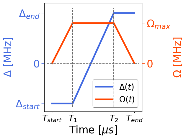
(a)

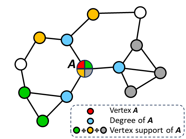
(b)

Figure 2: (a) Waveforms of $\Omega(t)$ and $\Delta(t)$ employed on adiabatic evolution. (b) Vertex support of A.

One of the primary variables to maintain adiabaticity is a minimum energy gap, $\delta_{\min}$, between a ground state and a first excited state coupled with the ground state during quantum evolution RSS+13 . The time $T$ required for sustaining adiabaticity should satisfy $T>1/\delta^{2}_{\min}$ FGGS00 . However, for graphs with complex configurations, the long-range Rydberg potential and large degeneracy in the ground states and the first excited states make it hard to identify the true minimum energy gap. Also, classical post-processing in our algorithm reduces the role of $\delta_{\min}$ in the adiabaticity. For these reasons, we can not use $\delta_{\min}$ as the metric of our strategy. Instead, we show that our strategy decreases $\delta_{\min}$ while evolving atoms forming a square lattice graph, which does not have ground state degeneracy.

II.3 Vertex support

The vertex support is the quantity that measures how many vertices are around a particular vertex. It was proposed by Balaji et al. BSK10 while suggesting heuristics for the MIS problem named as vertex support algorithm. To define the vertex support, let us introduce the undirected graph $G=(V,~{}E)$ again, where $V$ is the set of total vertex and $G$ is the set of total edges. Then, the neighborhood of the i-th vertex, denoted by $\mathcal{N}_{i}$, is the subset of $V$ and consists of vertices that are connected to i-th vertex. The degree of vertex i, $d_{i}$, is the cardinality of $\mathcal{N}_{i}$, i.e. $d_{i}=|\mathcal{N}_{i}|$. Then, the support of the i-th vertex, $s_{i}$, is the sum of degrees of elements in $\mathcal{N}_{i}$, i.e. $s_{i}=\sum_{j\in\mathcal{N}_{i}}d_{j}$. These whole definitions are described in 2(b). It is trivial that a vertex with large vertex support interacts more with other vertices than a vertex with relatively small vertex support. For approximating MIS, we reflect this point into the local detuning $\Delta_{i}$ in Eq. (3).

III Results

III.1 Adjusting local detunings according to vertex supports

The primary assumption in this paper is that a vertex with relatively more connection with others is less likely to be included in MIS. To apply this assumption to the Rydberg Hamiltonian, we employ vertex support to measure connectivity between vertices. Even though the degree is another connectivity measure, it was figured out that the vertex support works better than the degree in the numerical experiments. Of course, an atom that has more connection with others is more likely to be disturbed to be a Rydberg state implicitly by the strong Rydberg interaction in Eq. (4), we reflect the connectivity between atoms explicitly by adjusting the local detuning $\Delta_{i}$ in Eq. (3) atom by atom. This adjustment is accomplished by subtracting scaled vertex support from the $\Delta_{\mathrm{start}(\mathrm{end})}$. By doing so, the Rydberg state’s energy level alters according to the magnitude of each atom’s vertex support.

In fact, assigning different values in each local detuning transforms the system’s Hamiltonian from the MIS problem cost function to the MWIS problem cost function. Effectively, our approach can be conceptualized as a search for the weighted unit-disk graph of which MWIS is similar to the original graph’s MIS. Due to the adjusted local detunings by our strategy, this MWIS is easier to obtain by the adiabatic process than the original maximum independent sets.

To maximize the total Rydberg density $\langle n\rangle=\sum_{i\in V}\langle n_{i}\rangle$, we optimize a scaling factor of the vertex support $\epsilon$, $\Delta_{\mathrm{start}}$, and $\Delta_{\mathrm{end}}$ on Fig. 2(a). However, trials to maximize $\langle n\rangle$ can lead to consequences with enormous $\Delta_{\mathrm{end}}$, violating the independence constraint. Therefore, we adopt two classical post-processing strategies, the vertex reduction and the vertex addition in Ref. EKC+22 . After sampling evolved quantum states, the vertex reduction removes pairs of vertices, violating the independence constraint. Then, the vertex addition appends vertices to the independent set, which does not cause independence violations. The summary of our strategy is as follows.

1. For a given graph $G=(V,~{}E)$, calculate a vertex support of each vertex $\{s_{i}\}_{i\in V}$ and a mean of the vertex supports,

   $$\mathbb{E(\mathbf{s})}=\frac{1}{N}\sum_{i\in V}s_{i}.$$ (7)

2. Set each local detuning $\Delta_{i}$ of the $i$-th atom as follows,

   $$\Delta_{i,~{}\mathrm{start(end)}}=\Delta_{\mathrm{start(end)}}+(\mathbb{E(\mathbf{s})}-s_{i})\times\epsilon.$$ (8)

   We fixed several values throughout this paper: $\Omega_{\max}=2\pi\times 4$, $T_{1}=T_{\mathrm{end}}/7$, and $T_{2}=T_{\mathrm{end}}\times 6/7$ where $T_{1}$ and $T_{2}$ are come from Fig. 2(a). we empirically find that the initial values $\Delta_{\mathrm{start}}=-2\pi\times 8~{}\mathrm{MHz},~{}\Delta_{\mathrm{end}}=2\pi\times 10~{}\mathrm{MHz}$ with $\epsilon=1.5$ generally provide good results for the classes of graphs in our paper.

3. After enough time of evolution, sample the quantum state by basis {$|g_{i}\rangle,~{}|r_{i}\rangle$}.

4. Exploit vertex reduction and vertex addition on the sampled results sequentially. Then, calculate the total Rydberg density $\langle n\rangle$.

5. Optimize $\Delta_{\mathrm{start}},~{}\Delta_{\mathrm{end}}$, and $\epsilon$ to maximize $\langle n\rangle$ until the desired optimization threshold reached. More parameters can be added to deform the waveform of $\Delta(t)$ EKC+22 ; OLK+19 .

Note that because this strategy is based on the assumption mentioned at the beginning of this section, the sign of the optimized $\epsilon$ may be negative for some graphs, which contradicts the assumption. Nevertheless, these cases were about 2% of all simulated graphs. Also, the performance to approximate the maximum independent set raises for this case.

We obtain the value of the exact cost function by evolved quantum states without noise to identify the true power of this strategy. The gradient-free Nelder-Mead optimizer GH12 showed the best performance among several optimizers. Most of our numerical calculations were done with Bloqade.jl Blo23 , an open-source package developed for simulating a Rydberg atom based architecture.

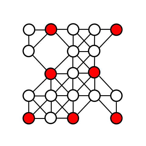
(a)

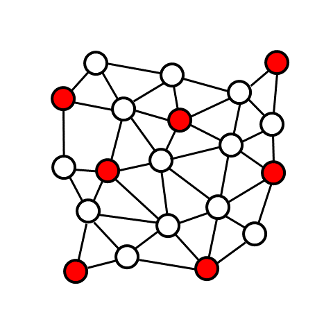
(b)

Figure 3: (a) A checkerboard graph with defects probability 0.2 and its maximum independent set is colored red. (b) A random graph of density of 3.0 and its maximum independent set is colored red.

III.2 Numerical simulations

In this section, we apply our strategy to two types of graphs, which are described in Fig. 3(a) and Fig. 3(b), one is a checkerboard graph with defects, and the other is a random graph generated by the procedure in Ref. SMA20 .

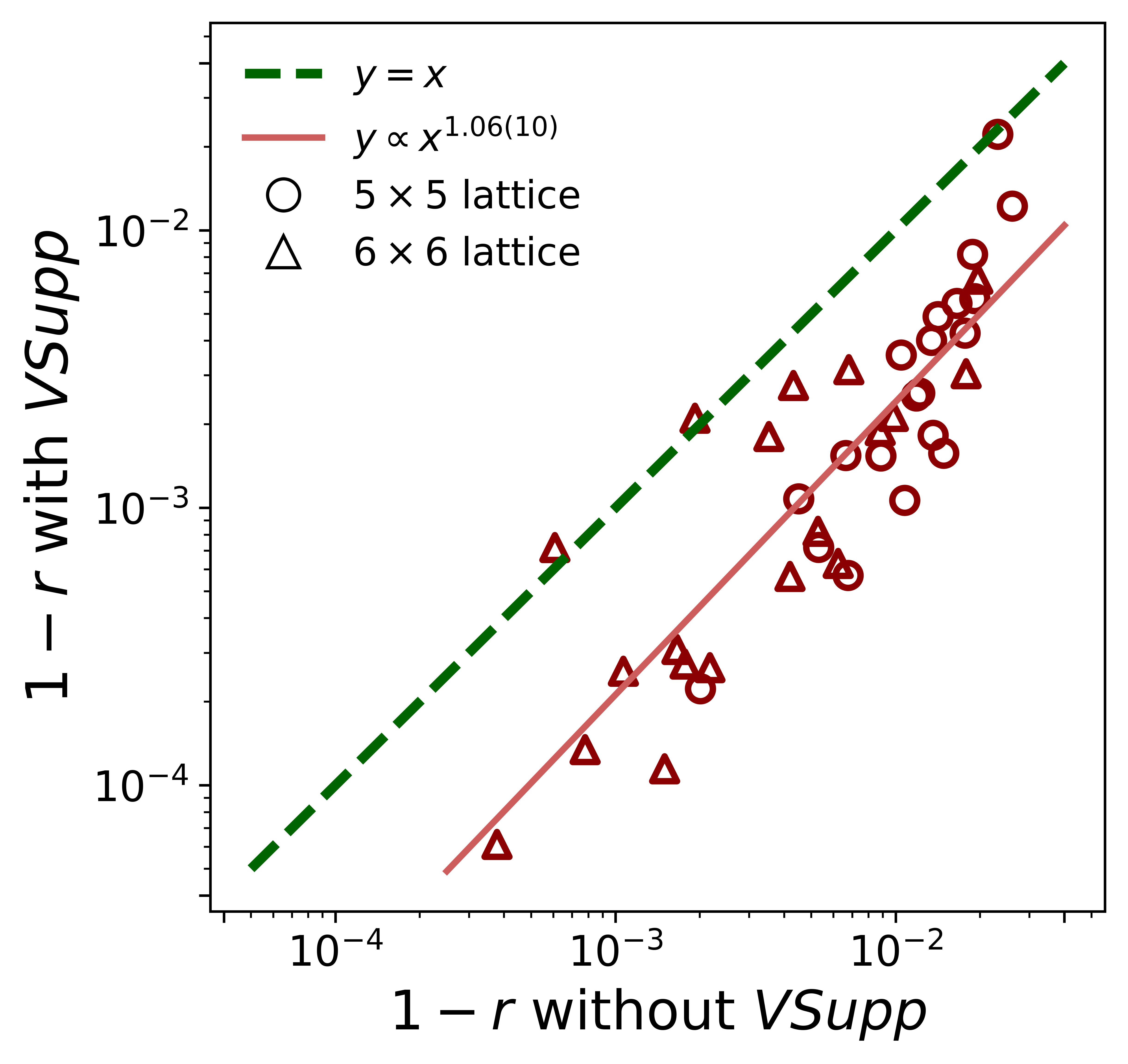
(a)

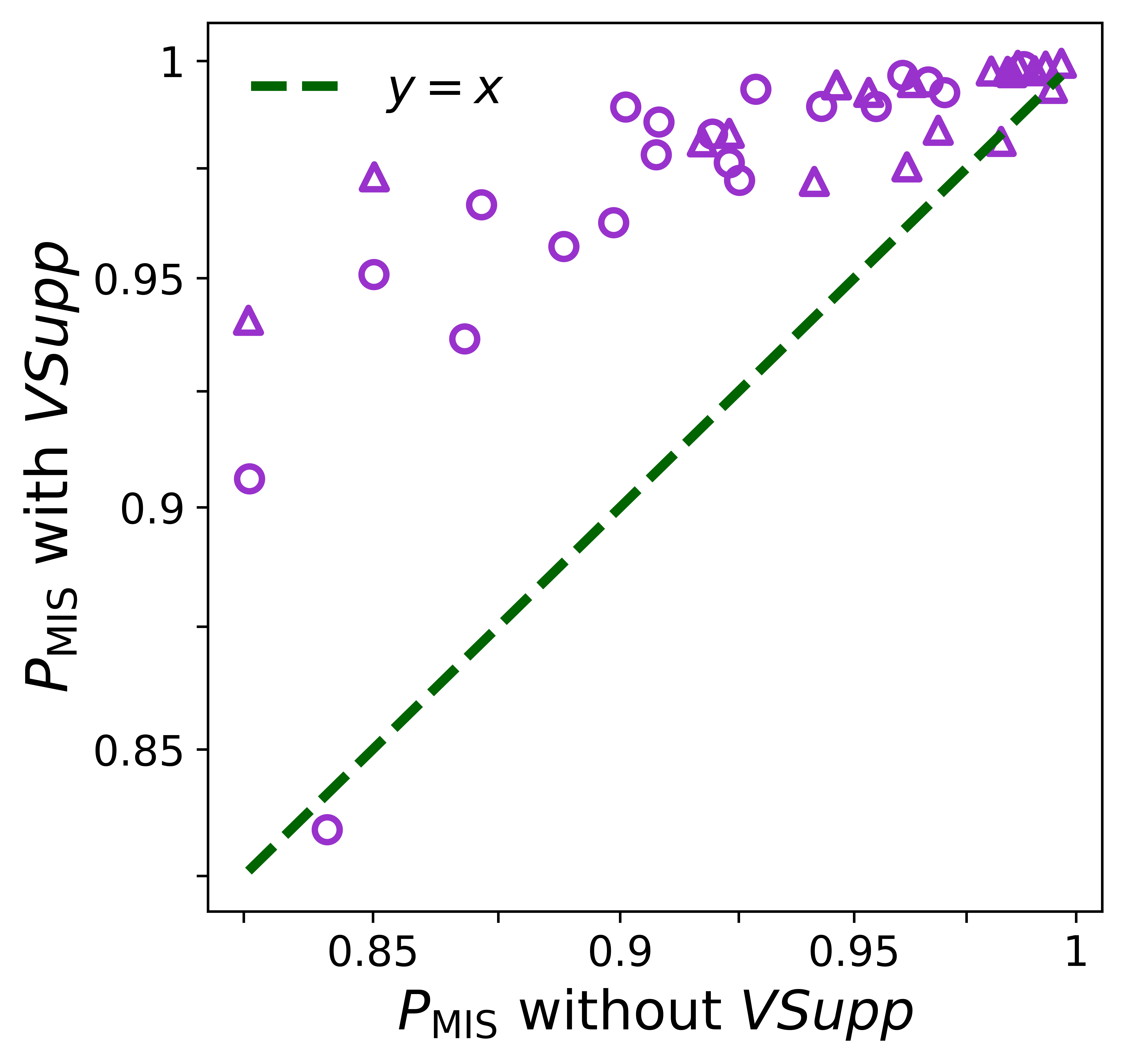
(b)

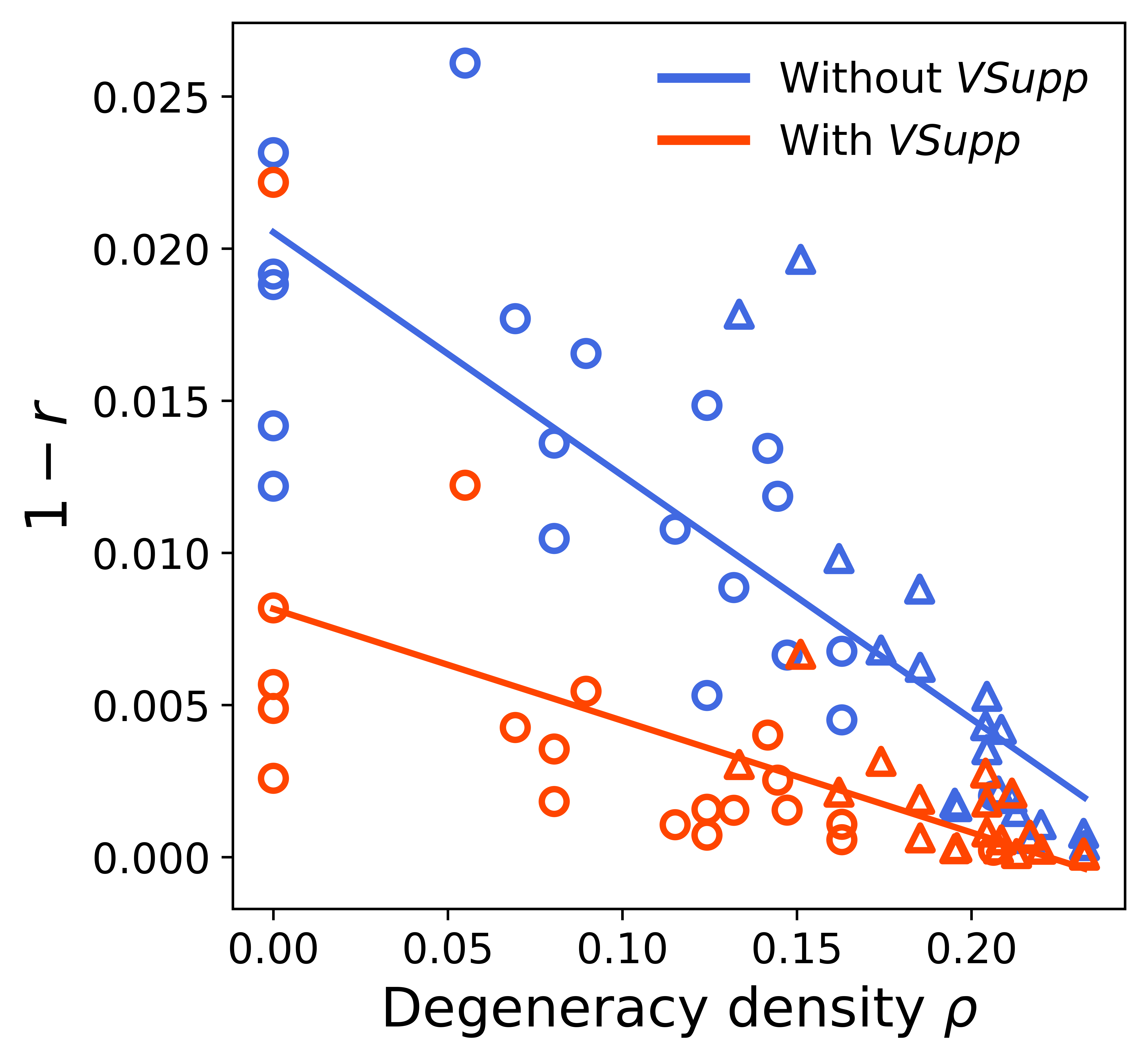
(c)

Figure 4: Optimized values after evolving randomly generated $5\times 5$ and $6\times 6$ checkerboard graphs with defects during $1~{}\mu s$, 20 instances for each size. The symbols to notate the size of graphs are showcased in Fig. 4(a). (a) The error rate $1-r$ ‘with VSupp’ versus ‘without VSupp’ is described by $\log$-$\log$ scale. The power law curve is employed to fit the results. (b) The probability of getting MIS with the strategy ‘without VSupp’ versus the probability of getting MIS with the strategy ‘with VSupp’ is described. (c) Comparing error rates $1-r$ between ‘without VSupp’ and ‘with VSupp’ according to the degeneracy density $\rho$. Linear fit of ‘without VSupp’ and ‘with VSupp’ is also described together.

To simulate a quantum evolution of atoms up to 29, which is intractable for classical computers, we neglect the Rydberg blockade violation of two atoms within a near range where the condition $V(|\vec{r}_{j}-\vec{r}_{k}|)\gg\Omega,\Delta$ is satisfied.

In the approximation scheme, we measure the performance of our strategy by approximation ratio $r$ and error rate $1-r$,

$$r=\frac{\langle n\rangle}{|I_{{\textnormal{MIS}}}|},$$ (9)

where the symbol $\langle n\rangle$ and $|I_{{\textnormal{MIS}}}|$ denotes the total Rydberg density and the cardinality of the MIS, respectively. It was suggested that the error rate $1-r$ and the degeneracy density $\rho=\log{(D_{|I_{{\textnormal{MIS}}}|})}/N$ is linearly dependent for the checkerboard graph with defects, where the $D_{|I_{{\textnormal{MIS}}}|}$ is the degeneracy of the maximum independent sets EKC+22 . We compare our strategy ‘with VSupp (vertex support)’, which optimizes $\{\Delta_{\mathrm{start}},\Delta_{\mathrm{end}},\epsilon\}$ and ‘without VSupp’ which optimizes $\{\Delta_{\mathrm{start}},\Delta_{\mathrm{end}}\}$ where both strategies encompass the classical post-processing.

The checkerboard graphs in this study connect nearest neighbor pairs and next nearest neighbor pairs. This next nearest connection makes us deal with non-planar graphs by Rydberg atom arrays. We set the nearest distance between two atoms as $4.5~{}\mu m$ where the Rydberg blockade radius $R_{b}\approx 7.74~{}\mu m$ by Eq. (6). We neglect the Rydberg blockade violation between nearest neighbors because $C_{6}/(4.5~{}\mu m)^{6}\approx 25.9\Omega\gg\Omega,\Delta$. 20% of total atoms in graphs are removed randomly to create defects.

After $1~{}\mu s$ time evolution of checkerboard graphs, the error rate considering vertex support (‘with VSupp’) is reduced compared to the error rate of ‘without VSupp’ through most error rate regions in Fig. 4(a). The power-law fitting between the error rate of ‘without VSupp’ and ‘with VSupp’ is $x^{1.06(10)}/3.16$, which represents high linearity between them. This evolution has sufficient adiabaticity because the probability of obtaining maximum independent sets, $P_{{\textnormal{MIS}}}$, is around 0.9 in Fig. 4(b). According to these figures, our strategy linearly reduces the error rate by three times for checkerboard graphs with defects when adiabaticity is sufficient. Notably, in Fig. 4(c), the error rate of both ‘with VSupp’ and ‘without VSupp’ shows weak linear dependency on the degeneracy density $\rho$, unlike the error rate of Ref. EKC+22 . This relatively weak linear dependency implies that the finite size effect plays a role due to the small size of our $5\times 5$ and $~{}6\times 6$ graphs, unlike the size of graphs in Ref. EKC+22 , which is up to 289 vertices. Furthermore, the cardinality of MIS in these graphs is 7 to 10, which is too small that the cardinality, rather than the degeneracy density $\rho$, might affect the error rate. Even though the tendency between the error rate and the degeneracy density is well conserved, verifying our strategy on larger graphs in actual experiments is necessary to clarify our strategy’s performance.

The random graphs, which are more general in practical problems, are characterized by the number of atoms and their density. Following the generation process in Ref. SMA20 , we generated random graphs with an exclusion radius of $4~{}\mu m$ for experimental realization and a density of 3.0 to make it possible to simulate a large number of atoms up to 28 with appropriate approximation. Also, we dismiss the Rydberg blockade violation inside $4\sqrt{2}~{}\mu m$ where $C_{6}/(4\sqrt{2}~{}\mu m)^{6}\approx 6.6\Omega>\Omega,\Delta$.

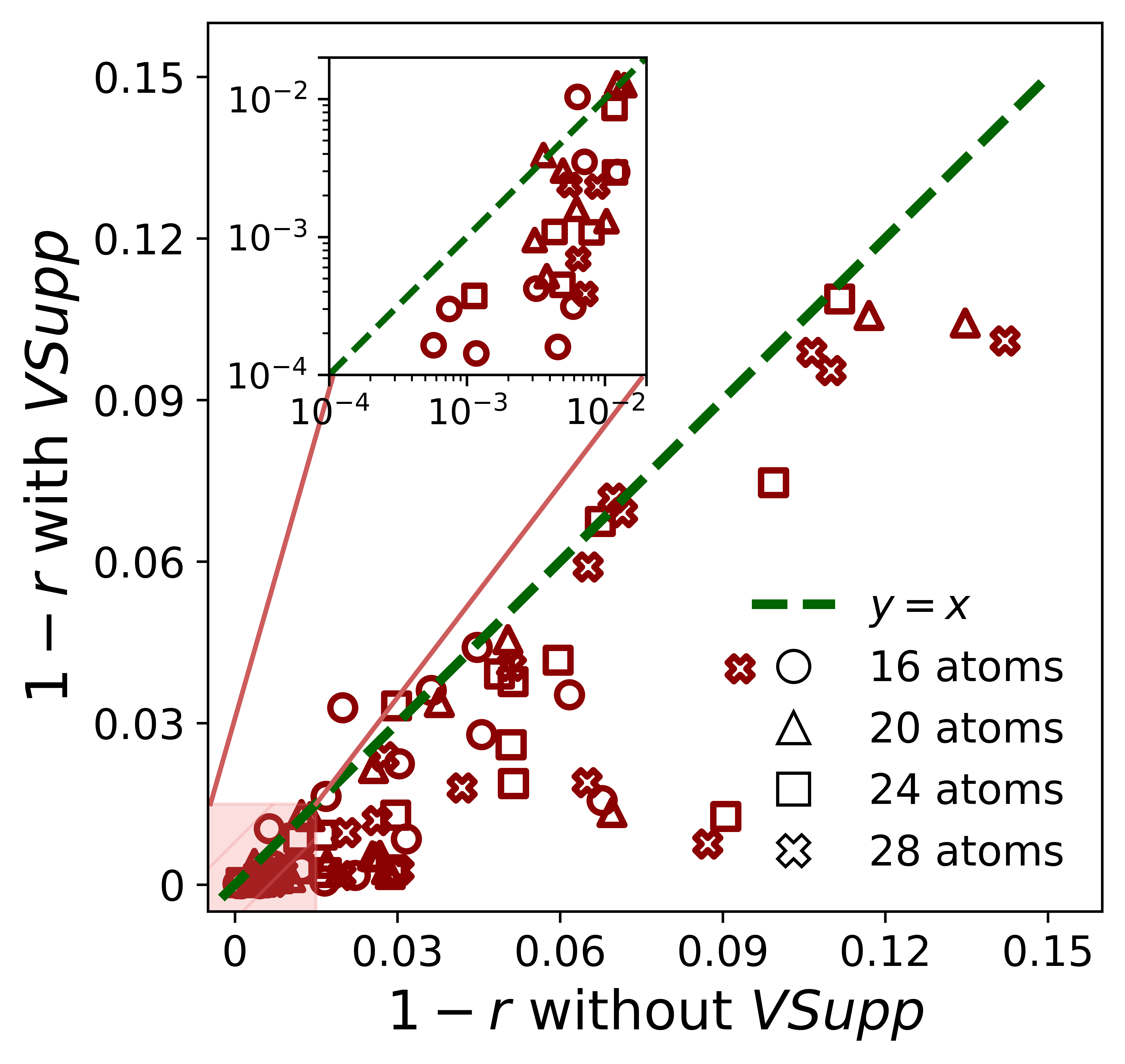
(a)

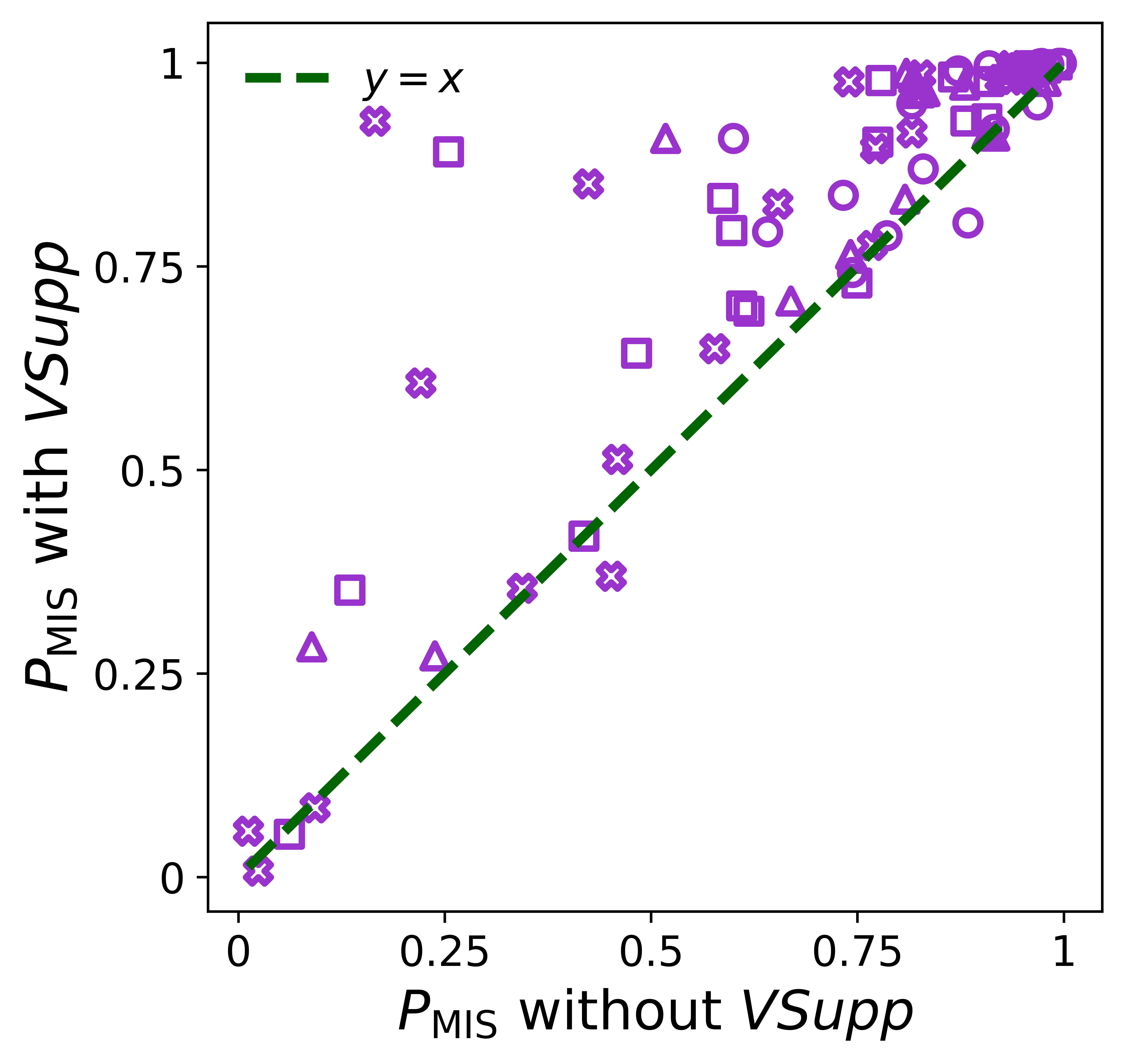
(b)

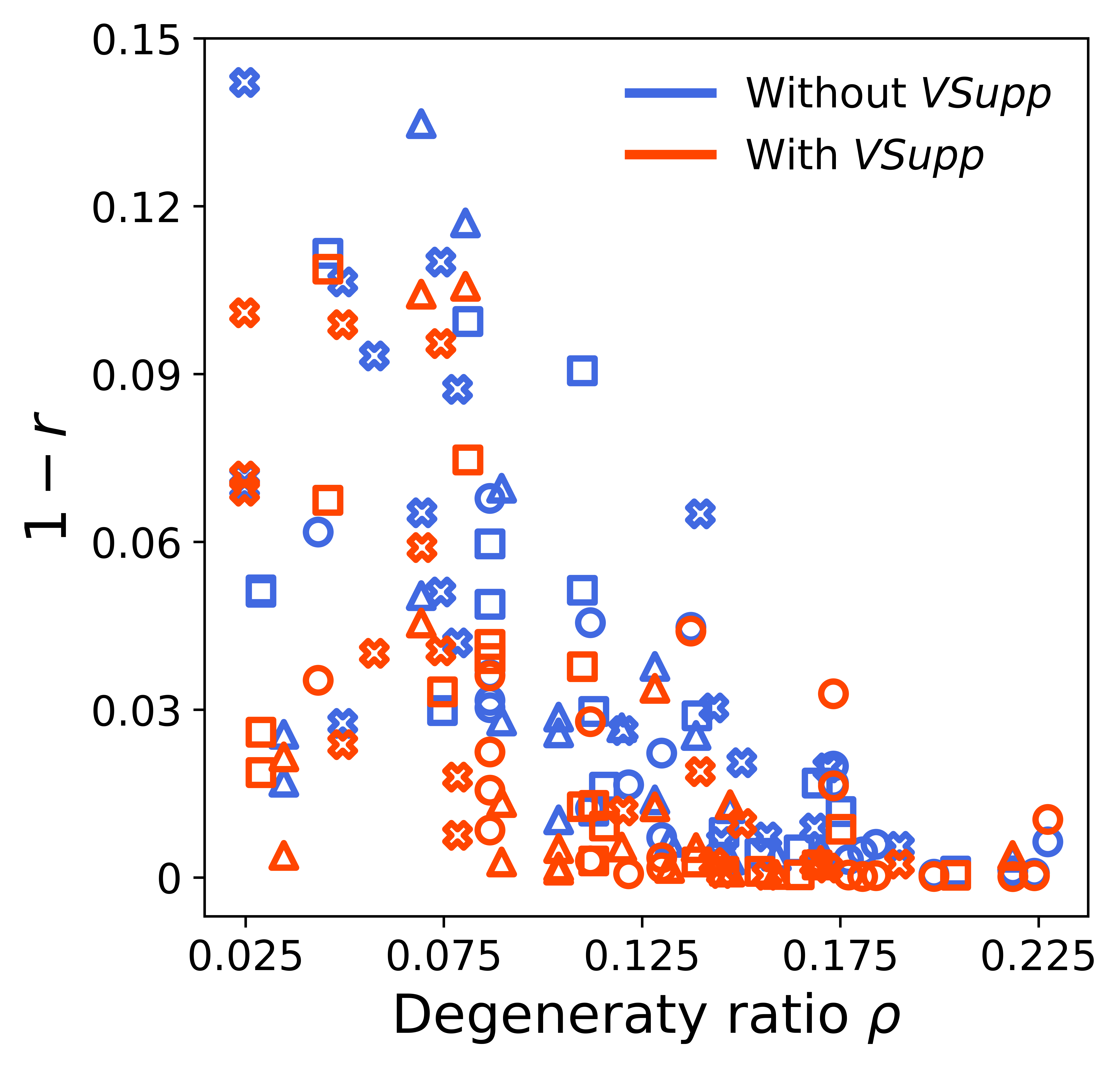
(c)

Figure 5: Optimized values after evolving random graphs of the density of 3.0 during $1~{}\mu s$. Twenty instances are simulated for each graph with 16, 20, 24, and 28 atoms. The symbols to notate the size of graphs are showcased in Fig. 5(a). (a) The error rate $1-r$ ‘without VSupp’ versus ‘with VSupp’ is described. The inset figure magnifies the area between $10^{-4}\leq x,y\leq 2\times 10^{-2}$ and utilizes $\log$-$\log$ scale. (b) The probability of getting MIS with the strategy ‘without VSupp’ versus the case of ‘with VSupp’ is described. (c) Comparing error rates $1-r$ between ‘without VSupp’ and the case of ’with VSupp’ according to the degeneracy density $\rho$.

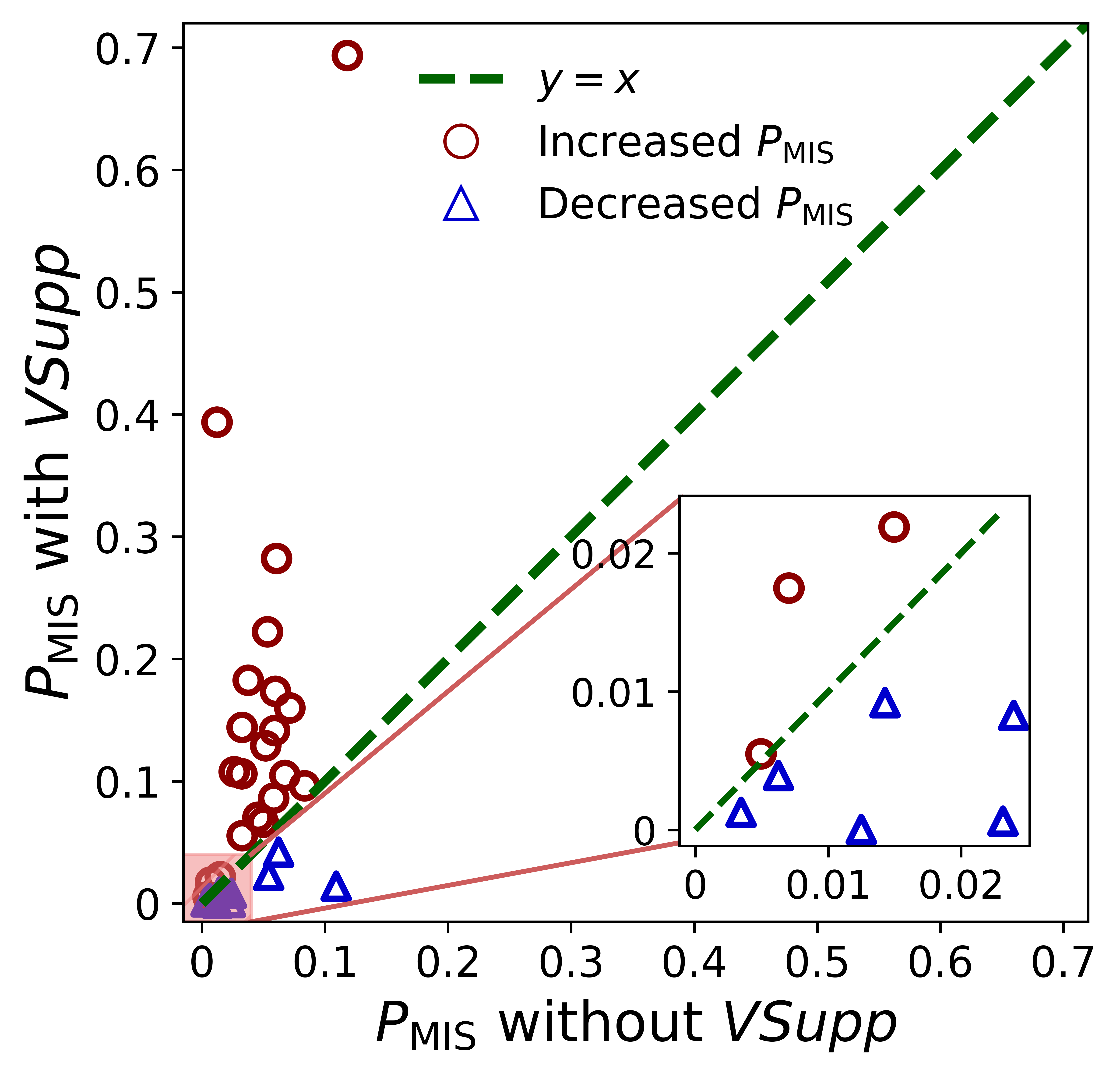
(a)

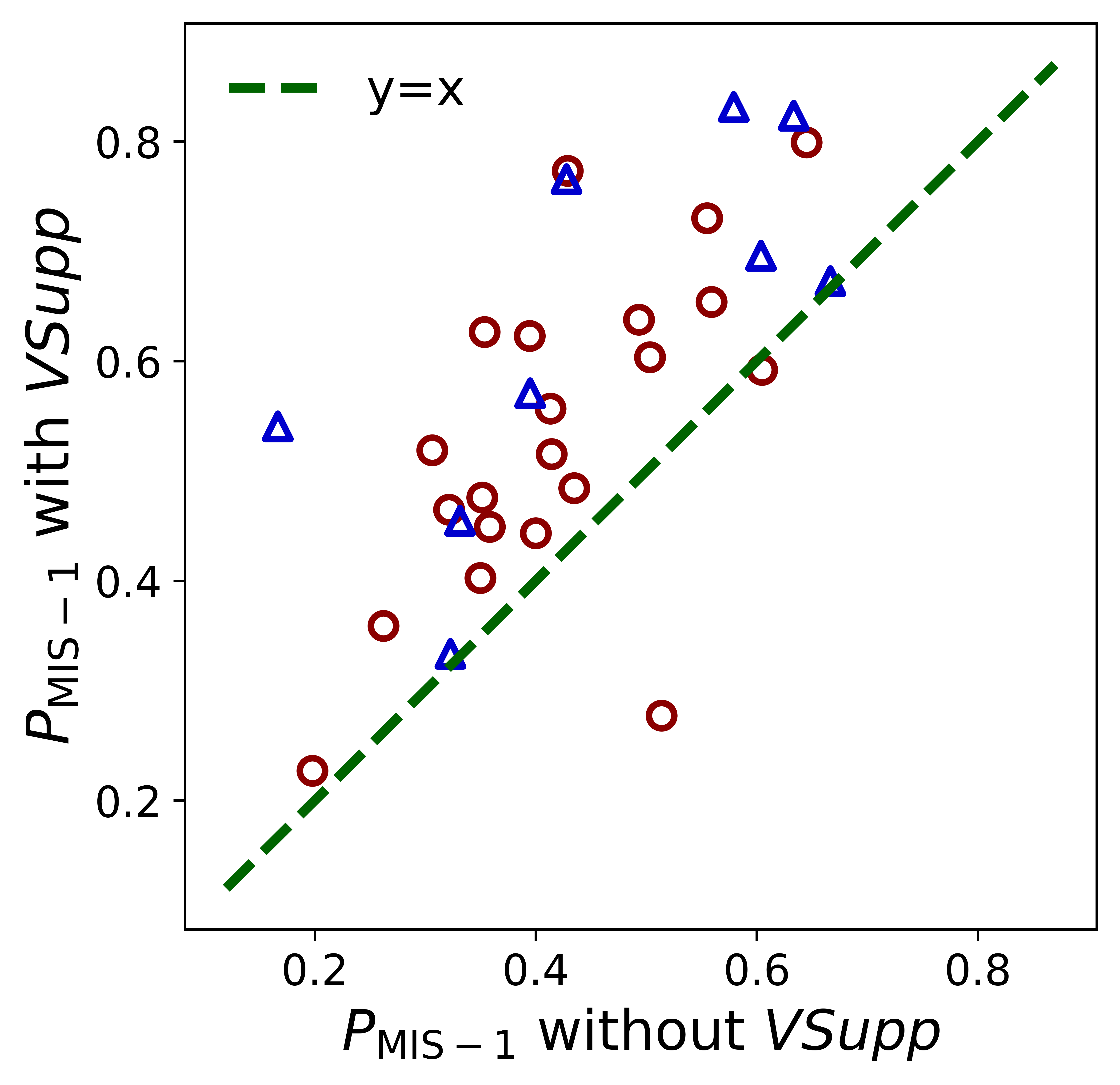
(b)

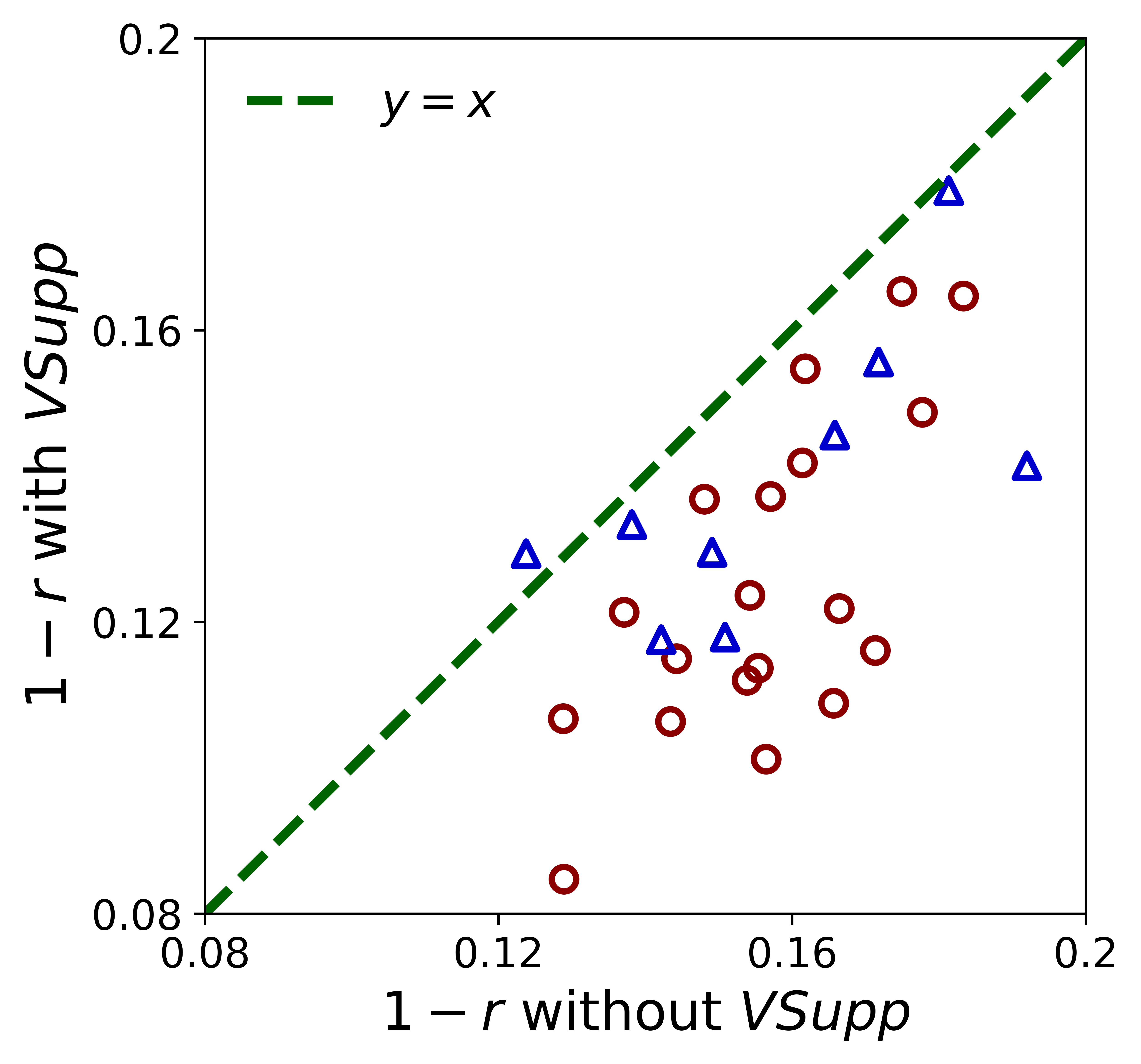
(c)

Figure 6: Optimized values after evolving random graphs of the density of 3.0, ground degeneracy $D_{{\textnormal{MIS}}}=1$, during $0.4~{}\mu s$. Thirty instances are simulated where the number of vertices is 28. The red circle indicates the instances in which $P_{{\textnormal{MIS}}}$ are increased, and the blue triangle indicates the instances in which $P_{{\textnormal{MIS}}}$ are decreased. (a) The probability of getting MIS with the strategy ‘without VSupp’ versus $P_{{\textnormal{MIS}}}$ with the strategy ‘with VSupp’ is described. The inset figure magnifies the area between $0\leq x,y\leq 0.2$. (b) The probability of getting the first excited state, which is named as $P_{{\textnormal{MIS}}-1}$, with the strategy ‘without VSupp’ versus the case of ’with VSupp’ is described. (c) The error rate $1-r$ with the strategy ‘without VSupp’ versus the case of ‘with VSupp’ is described.

After $1~{}\mu s$ time evolution of several random graphs, points in Fig. 5(a) are dominantly distributed under the line $y=x$ through $10^{-4}\leq x\leq 10^{-1}$, which exhibits the success of our strategy. Some instances show a dramatic decrease in the error rate even for the high error rate with the strategy ‘without VSupp’. Although the evolution time is identical and the range of degeneracy ratio is similar to that of Fig. 4, the range of error rate and the $P_{{\textnormal{MIS}}}$ is relatively more expansive than that of Fig. 4 which shows that the random graphs of the density of 3.0 are generally complex to solve than the checkerboard graphs with defects. In conclusion, 92.5% of the total instances’ error rate is decreased by considering the vertex support. Both ‘without VSupp’ and ‘with VSupp’ indicate weaker linear dependency on the degeneracy ratio than the dependency in Fig. 4(c).

To demonstrate the performance of our strategy in classically intractable larger graphs, we apply our strategy to more challenging graphs with shorter time, which results in less adiabaticity during evolution. In Fig. 6, 30 random graphs with ground degeneracy $D_{|I_{\textnormal{MIS}}|}=0$ are chosen because there is a tendency that the graphs with small degeneracy ratio $\rho$ have relatively large error rate $1-r$ on Fig. 4(c), 5(c).

With less adiabaticity, the $P_{{\textnormal{MIS}}}$ decreased for 9 out of 30 random graphs, which is described in Fig. 6(a), where $P_{{\textnormal{MIS}}}$ of ‘without VSupp’ is mostly under $10^{-1}$. However, in Fig. 6(b), our strategy increased the probability of getting the first excited state, $P_{{\textnormal{MIS}}-1}$, for almost every graph. As a result, the mean error rate of ‘without VSupp’, $0.16\pm 0.02$, reduces to $0.12\pm 0.03$ by our strategy in Fig. 6(c). Notably, the error rate is decreased even for the graphs in which $P_{{\textnormal{MIS}}}$ is decreased. This decrease implies that our strategy can be an excellent suggestion to approximate more challenging graphs, which we cannot sustain sufficient adiabaticity with current technology.

III.3 Preparing 2D cat state

Although we find MIS by adiabatic evolution, we are uncertain about obtain a physical quantum ground state through the above scheme because of the classical post-processing after measurements. The classical post-processing is necessary to obtain MIS in our process since maximizing the total Rydberg density $\langle n\rangle$ by optimizing $\Delta_{\mathrm{end}}$ leads all atoms to become the Rydberg state. Otherwise, if we know the ground states of the Hamiltonian before evolution, we can prepare the ground states more easily by maximizing $P_{{\textnormal{MIS}}}$.

Because a quantum superposition is hard to directly prepare by adjusting local detunings, our scheme is beneficial when the desired ground state is a superposition of two computational states. For example, the cat state is a superposition of two opposed states, such as $|000\dotsi 0\rangle$ and $|111\dotsi 1\rangle$. The cat state can be used to benchmark quantum hardware OLK+19 ; SXL+17 ; SUP+17 , quantum error correction SDM+22 , and quantum network HBW+19 . For the Rydberg atom arrays, the 1D cat state $(|010\dotsi 1\rangle+|101\dotsi 0\rangle)/\sqrt{2}$ is experimentally prepared up to 20 atoms with fidelity $F=\langle\psi_{{\textnormal{CAT}}}|\rho|\psi_{{\textnormal{CAT}}}\rangle\geq 0.5$ by applying local detunings at the edges of configuration OLK+19 . In this section, we prepare the 2D cat state described in Fig. 7 by applying local detunings according to the vertex support as a concept to quantify connectivity. The $4\times 4$ square lattice was used to demonstrate the increase in fidelity by our strategy. There was no approximation during quantum evolution since the distance between two adjacent atoms is long enough.

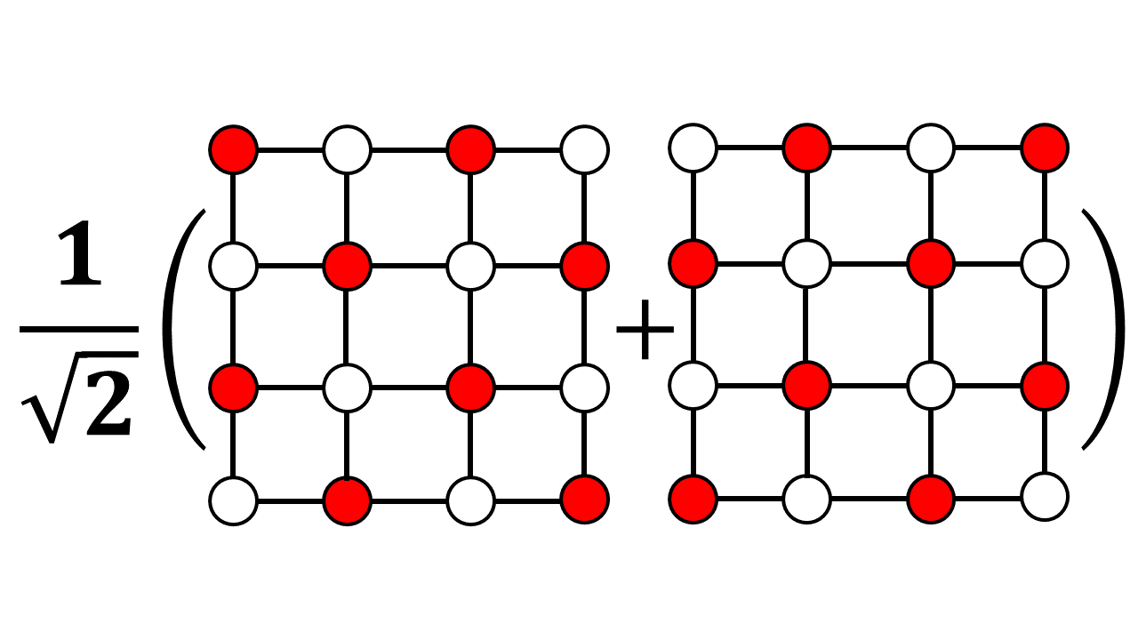
Figure 7: Cat state on a $4\times 4$ square lattice where nearest neighbor vertices are connected.

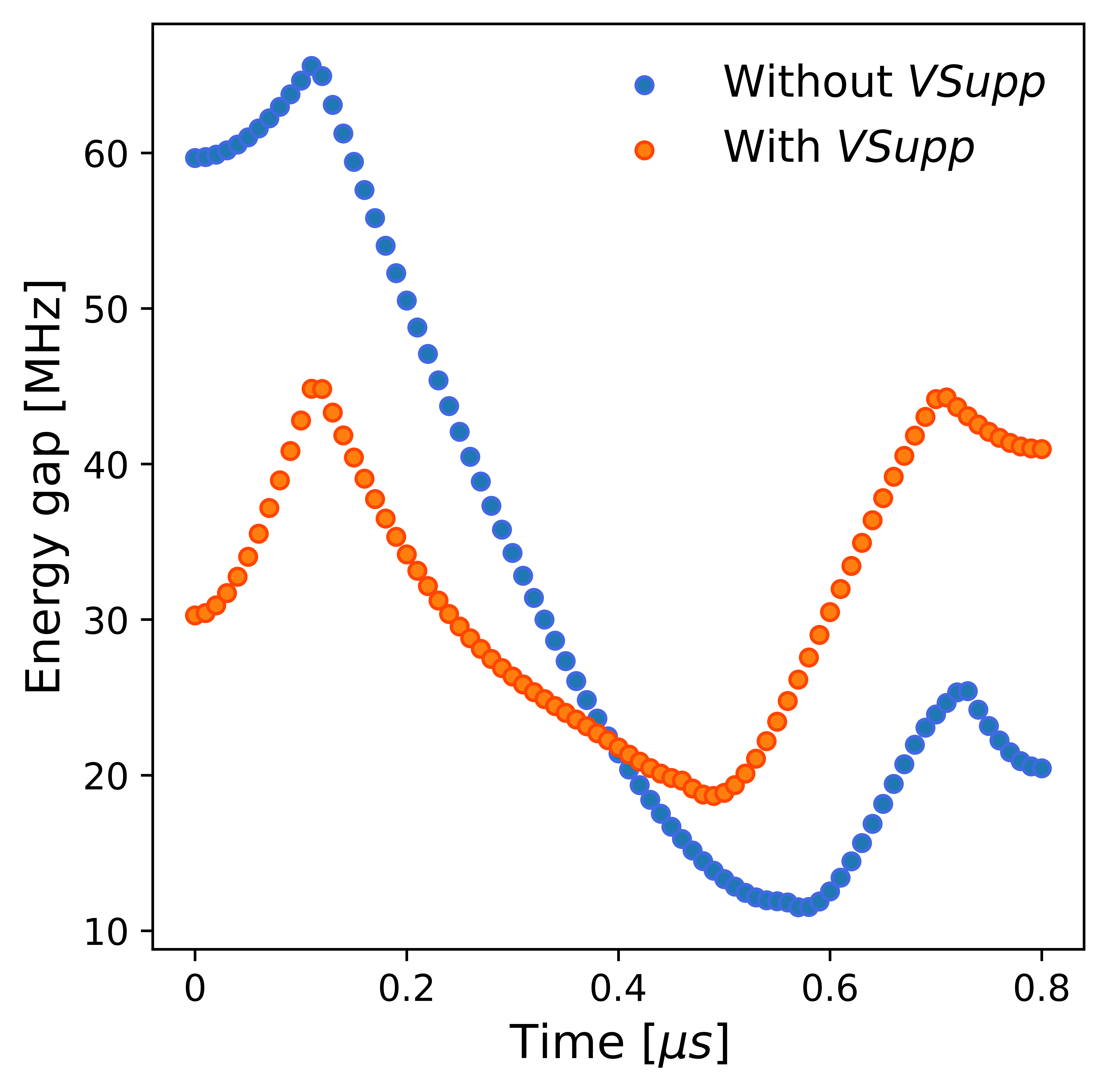
Figure 8: Comparing the energy gap between the ground state and the coupled first excited state of ‘without VSupp’ and ‘with VSupp’ according to evolution time.

During $0.8~{}\mu s$ time evolution, the energy gap between the ground state and the coupled first excited state is plotted in Fig. 8. Our strategy raises the minimum energy gap $\delta_{\min}$ from 11.5 to 18.7. This increase in adiabaticity influences the fidelity between the cat state and the evolved quantum state. The fidelity between them increases from 0.68 to 0.90. Notably, the optimized $\epsilon$ multiplied by the vertex support is negative, which is opposed to the default sign. This negative sign is because, for the square lattice in Fig. 7, the vertices at the edges are more likely to be in a Rydberg state than those with more connection with others. This consequence implies that whether or not our assumption can not precisely recommend the ground states, its ability to quantify connectivity works successfully. The vertex support quantifies connectivity well and helps to prepare some particular quantum ground states.

IV Conclusions and Discussions

We proposed the new approximation strategy for finding unit-disk maximum independent sets on Rydberg atom arrays. This strategy assumes that a vertex connected more with other vertices is less likely to be in maximum independent sets. The vertex support quantifies connectivity between vertices, and we apply this quantity to the Rydberg Hamiltonian. This approach successfully reduces the error rate three times for the checkerboard graphs with defects. For random graphs with the density of 3.0, the error rate is successfully decreased regardless of the amount of adiabaticity and the probability of obtaining ground states. Furthermore, our strategy can be extended to solving arbitrarily connected maximum independent set GMOS23 or maximum weight independent set NLW+23 on Rydberg atom arrays because our assumption does not rely on the property of the unit-disk graph.

Beyond QAA, our strategy can be applied to QAOA by encoding an amount of potential inclusion into the cost function EKC+22 . In fact, QAOA may be more suitable for our strategy than the quantum adiabatic algorithm because of its diabatic approach to preparing ground states ZWC+20 . Even though the MWIS cost function produced after the strategy facillitates the population of the first excited state, this result can lead to more population of the ground state after the minimum energy gap by diabatic evolution, as discussed in  SRN+12 ; CFL+14 . In our numerical calculations, some drastic increase of $P_{{\textnormal{MIS}}}$ for complex graphs supports this argument. Because our strategy is based on the assumption, finding new weights which work better in representing connectivity between vertices will be our future research.

Besides the role of vertex support in finding MIS on Rydberg atom arrays, it helps prepare specific quantum ground states if there is no classical post-processing. Applying this process to the cat state on a $4\times 4$ square lattice increases the minimum energy gap during the evolution. The fidelity between the prepared ground state and the 2D cat state rises from 0.68 to 0.90. Furthermore, it can be applied to other lattices such as kagome lattice and honeycomb lattice. Our strategy to increase the fidelity of the quantum many-body ground state will be fruitful in several areas, such as quantum error correction SDM+22 and quantum communication HBW+19 .

Furthermore, our concept of using vertex support in preparing quantum many-body ground state or obtaining ground energy is adaptable to various platforms and problems in a similar way. Exploring other applications of our logic is also possible since our assumption is confined to the maximum independent set problem.

References

- (1) T. Albash and D. A. Lidar, “Adiabatic quantum computation,” Rev. Mod. Phys. 90, 015002 (2018).
- (2) J. Roland and N. J. Cerf, “Quantum search by local adiabatic evolution,” Phys. Rev. A 65, 042308 (2002).
- (3) E. Farhi, J. Goldstone, and S. Gutmann, “Quantum Adiabatic Evolution Algorithms with Different Paths,” arXiv:quant-ph/0208135 (2002).
- (4) S. Ebadi, T. T. Wang, H. Levine, A. Keesling, G. Semeghini, A. Omran, D. Bluvstein, R. Samajdar, H. Pichler, W. W. Ho, S. Choi, S. Sachdev, M. Greiner, V. Vuletić, and M. D. Lukin, “Quantum phases of matter on a 256-atom programmable quantum simulator,” Nature 595, 227 (2021).
- (5) T. Hogg and D. Portnov, “Quantum optimization,” Inf. Sci. 128, 181 (2000).
- (6) A. M. Childs, E. Farhi, J. Goldstone, and S. Gutmann, “Finding cliques by quantum adiabatic evolution,” Quantum Inf. Comput. 2, 181 (2002).
- (7) A. Schrijver, “On the History of Combinatorial Optimization (Till 1960),” Handbooks in Operations Research and Management Science 12, 1 (2005).
- (8) E. Farhi, J. Goldstone, S. Gutmann, J. Lapan, A. Lundgren, and D. Preda, “A Quantum Adiabatic Evolution Algorithm Applied to Random Instances of an NP-Complete Problem,” Science 292, 472 (2001).
- (9) Roth, Marco and Moll, Nikolaj and Salis, Gian and Ganzhorn, Marc and Egger, Daniel J. and Filipp, Stefan and Schmidt, Sebastian, “Adiabatic quantum simulations with driven superconducting qubits,” Phys. Rev. A 99, 022323 (2019).
- (10) Qi, Lu and Reed, Evan C. and Brown, Kenneth R., “Adiabatically controlled motional states of a and trapped-ion chain cooled to the ground state,” Phys. Rev. A 108, 013108 (2023).
- (11) P. Scholl, M. Schuler, H. J. Williams, A. A. Eberharter, D. Barredo, K.-N. Schymik, V. Lienhard, L.-P. Henry, T. C. Lang, T. Lahaye, A. M. Läuchli, and A. Browaeys, “Quantum simulation of 2D antiferromagnets with hundreds of Rydberg atoms,” Nature 595, 233 (2021).
- (12) A. Omran, H. Levine, A. Keesling, G. Semeghini, T. T. Wang, S. Ebadi, H. Bernien, A. S. Zibrov, H. Pichler, S. Choi, J. Cui, M. Rossignolo, P. Rembold, S. Montangero, T. Calarco, M. Endres, M. Greiner, V. Vuletić, and M. D. Lukin, “Generation and manipulation of Schrödinger cat states in Rydberg atom arrays,” Science 365, 570 (2019).
- (13) H. Pichler, S.-T. Wang, L. Zhou, S. Choi, and M. D. Lukin, “Quantum Optimization for Maximum Independent Set Using Rydberg Atom Arrays,” arXiv:1808.10816 (2018).
- (14) H. Pichler, S.-T. Wang, L. Zhou, S. Choi, M. D. Lukin, “Computational complexity of the Rydberg blockade in two dimensions,” arXiv:1809.04954 (2018).
- (15) J. Wurtz, P. L. S. Lopes, C. Gorgulla, N. Gemelke, A. Keesling, and S. Wang, “Industry applications of neutral-atom quantum computing solving independent set problems,” arXiv:2205.08500 (2022).
- (16) S. Weber, J. G. Andrews, and N. Jindal, “An Overview of the Transmission Capacity of Wireless Networks,” IEEE Trans. Commun. 58, 3593 (2010).
- (17) S. Butenko, Maximum independent set and related problems, with applications (University of Florida, 2003).
- (18) B. N. Clark, C. J. Colbourn, and D. S. Johnson, “Unit disk graphs,” Discrete Math. 86, 165 (1990).
- (19) X. Wu, X. Liang, Y. Tian, F. Yang, C. Chen, Y.-C. Liu, M. K. Tey, and L. You, “A concise review of Rydberg atom based quantum computation and quantum simulation,” Chin. Phys. B 30, 020305 (2021).
- (20) M. Kim, K. Kim, J. Hwang, E.-G. Moon, and J. Ahn, “Rydberg quantum wires for maximum independent set problems,” Nat. Phys. 18, 755 (2022).
- (21) M.-T. Nguyen, J.-G. Liu, J. Wurtz, M. D. Lukin, S.-T. Wang, and H. Pichler, “Quantum Optimization with Arbitrary Connectivity Using Rydberg Atom Arrays,” PRX Quantum 4, 010316 (2023).
- (22) K. Goswami, R. Mukherjee, H. Ott, and P. Schmelcher, “Solving optimization problems with local light shift encoding on Rydberg quantum annealers,” arXiv:2308.07798 (2023).
- (23) B. F. Schiffer, D. S. Wild, N. Maskara, M. Cain, M. D. Lukin, and R. Samajdar, “Circumventing superexponential runtimes for hard instances of quantum adiabatic optimization,” arXiv:2306.13131 (2023).
- (24) M. Cain, S. Chattopadhyay, J.-G. Liu, R. Samajdar, H. Pichler, and M. D. Lukin, “Quantum speedup for combinatorial optimization with flat energy landscapes,” arXiv:2306.13123 (2023).
- (25) S. Ebadi, A. Keesling, M. Cain, T. T. Wang, H. Levine, D. Bluvstein, G. Semeghini, A. Omran, J.-G. Liu, R. Samajdar, X.-Z. Luo, B. Nash, X. Gao, B. Barak, E. Farhi, S. Sachdev, N. Gemelke, L. Zhou, S. Choi, H. Pichler, S.-T. Wang, M. Greiner , V. Vuletić, and M. D. Lukin, “Quantum optimization of maximum independent set using Rydberg atom arrays,” Science 376, 1209 (2022).
- (26) R. S. Andrist, M. J. A. Schuetz, P. Minssen, R. Yalovetzky, S. Chakrabarti, D. Herman, N. Kumar, G. Salton, R. Shaydulin, Y. Sun, M. Pistoia, and H. G. Katzgraber, “Hardness of the maximum-independent-set problem on unit-disk graphs and prospects for quantum speedups,” Phys. Rev. Research 5, 043277 (2023).
- (27) G. K. Das, M. De, S. Kolay, S. C. Nandy, and S. Sur-Kolay, “Approximation algorithms for maximum independent set of a unit disk graph,” Inf. Process. Lett. 115, 439 (2015).
- (28) S. Balaji, V. Swaminathan, and K. Kannan, “A Simple Algorithm to Optimize Maximum Independent Set,” Advanced Modeling and Optimization 12, 107 (2010).
- (29) Hannes Bernien, Sylvain Schwartz, Alexander Keesling, Harry Levine, Ahmed Omran, Hannes Pichler, Soonwon Choi, Alexander S. Zibrov, Manuel Endres, Markus Greiner, Vladan Vuletić, and Mikhail D. Lukin “Probing many-body dynamics on a 51-atom quantum simulator,” Nature 551, 579 (2017).
- (30) H. Labuhn, D. Barredo, S. Ravets, S. de Léséleuc, T. Macrì, T. Lahaye, and A. Browaeys, “Tunable two-dimensional arrays of single Rydberg atoms for realizing quantum Ising models,” Nature 534, 667 (2016).
- (31) E. Farhi, J. Goldstone, and S. Gutmann, “A quantum approximate optimization algorithm,” arXiv:1411.4028 (2014).
- (32) L. Zhou, S.-T. Wang, S. Choi, H. Pichler, and M. D. Lukin, “Quantum Approximate Optimization Algorithm: Performance, Mechanism, and Implementation on Near-Term Devices,” Phys. Rev. X 10, 021067 (2020).
- (33) P. Richerme, C. Senko, J. Smith, A. Lee, S. Korenblit, and C. Monroe, “Experimental performance of a quantum simulator: Optimizing adiabatic evolution and identifying many-body ground states,” Phys. Rev. A 88, 012334 (2013).
- (34) E. Farhi, J. Goldstone, S. Gutmann, and M. Sipser, “Quantum Computation by Adiabatic Evolution,” arXiv:quant-ph/0001106 (2000).
- (35) F. Gao and L. Han, “Implementing the Nelder-Mead simplex algorithm with adaptive parameters,” Comput. Optim. Appl. 51, 259 (2012).
- (36) QuEraComputing, Bloqade.jl: Package for the quantum computation and quantum simulation based on the neutral-atom architecture (2023).
- (37) M. F. Serret, B. Marchand, and T. Ayral, “Solving optimization problems with Rydberg analog quantum computers: Realistic requirements for quantum advantage using noisy simulation and classical benchmarks,” Phys. Rev. A 102, 052617 (2020).
- (38) C. Song, K. Xu, W. Liu, C.-p.Yang, S.-B. Zheng, H. Deng, Q. Xie, K. Huang, Q. Guo, L. Zhang, P. Zhang, D. Xu, D. Zheng, X. Zhu, H. Wang, Y.-A. Chen, C.-Y. Lu, S. Han, and J.-W. Pan, “10-Qubit Entanglement and Parallel Logic Operations with a Superconducting Circuit,” Phys. Rev. Lett. 119, 180511 (2017).
- (39) D. V. Sychev, A. E. Ulanov, A. A. Pushkina, M. W. Richards, I. A. Fedorov, and A. I. Lvovsky, “Enlargement of optical Schrödinger’s cat states,” Nat. Photon. 11, 379 (2017).
- (40) Schlegel, David S. and Minganti, Fabrizio and Savona, Vincenzo, “Quantum error correction using squeezed Schrödinger cat states,” Phys. Rev. A 106, 022431 (2022).
- (41) Hacker, Bastian and Welte, Stephan and Daiss, Severin and Shaukat, Armin and Ritter, Stephan and Li, Lin and Rempe, Gerhard, “Deterministic creation of entangled atom–light Schrödinger-cat states,” Nat. Photon. 13, 110 (2019).
- (42) Somma, Rolando D. and Nagaj, Daniel and Kieferová, Mária, “Quantum Speedup by Quantum Annealing,” Phys. Rev. Lett. 109, 050501 (2012).
- (43) Crosson, Elizabeth and Farhi, Edward and Lin, Cedric Yen-Yu and Lin, Han-Hsuan and Shor, Peter, “Different Strategies for optimization Using the Quantum Adiabatic Algorithm,” arXiv:quant-ph/1401.7320 (2014).